Analysis of LULC and Urban Thermal Variations in Industrial Cities Using Earth Observation Indices and Machine Learning: A Case Study of Gujranwala, Pakistan

Abstract

Rapid urbanization and industrial development have significantly altered land use and cover across the globe, intensifying urban thermal environments and exacerbating the urban heat island (UHI) effect. Gujranwala, Pakistan, represents an industrial growth that has driven substantial land use/land cover (LULC) changes and temperature increases; however, the directional and distance-based patterns of these changes remain unquantified. Therefore, this study is conducted to examine spatiotemporal changes in LULC and variations in the Urban Thermal Field Variation Index (UTFVI) between 2001 and 2021 and to project future scenarios for 2031 and 2041 using (1) Earth Observation Indices (EOIs) with machine learning (ML) classifiers (Random Forest) for precise LULC mapping through the Google Earth Engine (GEE) platform, (2) Cellular Automata–Artificial Neural Networks (CA-ANNs) for future scenario projection, and (3) Gradient Directional Analysis (GDA) to quantify directional (16-axis) and distance-based (concentric zones) patterns of urban expansion and thermal variation from 2001–2021. The study revealed significant LULC changes, with built-up areas expanding by 7.5% from 2001 to 2021, especially in the east, northeast, and southeast directions within a 20 km radius. Due to urban encroachment, vegetation and cropland decreased by 1.47% and 1.83%, respectively. The urban thermal environment worsened, with the highest land surface temperature (LST) rising from 41 °C in 2001 to 55 °C in 2021. Additionally, the UTFVI showed expanding areas under the ‘strong’ and ‘strongest’ categories, increasing from 30.58% in 2001 to 33.42% in 2041. Directional analysis highlighted severe thermal stress in the southern and southwestern areas linked to industrial activities and urban sprawl. This integrated approach provides a template for analyzing urban thermal environments in developing cities, supporting targeted mitigation strategies through direction- and distance-specific planning interventions to mitigate UHI impacts.

1. Introduction

The rapid urbanization and industrialization of cities worldwide have led to significant changes in LULC [1,2,3]. These changes are crucial in shaping urban environments, particularly in industrial cities where the hasty expansion of built-up areas, industrial zones, and transportation networks significantly alter natural landscapes, ecological balances, and thermal characteristics [4,5,6,7]. The transformation of LULC in urban areas alters local climate patterns, leading to higher land surface temperatures (LSTs) and the formation of urban heat islands (UHIs) observed as elevated temperatures in urban cores compared to rural surroundings [8,9]. These UHI patterns are exacerbated by factors such as heat emissions, reduced vegetation, and impervious surfaces [10]. These thermal variations pose environmental sustainability challenges [11,12], including increased energy consumption, deteriorating air–water quality, altered microclimates, ecological degradation, loss of biodiversity, and adverse health impacts [13,14].

Industrial cities exhibit pronounced UHI intensity due to concentrated anthropogenic heat sources (e.g., factories, traffic) and land use changes [15,16]. The presence of manufacturing units, heavy vehicular activity, and high-density urban settlements contributes to localized temperature anomalies [17]. These UHI patterns result from the urban heat island effect (UHIE), a process amplified by industrial energy consumption, waste heat emissions [18], and loss of vegetated cooling surfaces [19]. Previous studies have highlighted that industrial areas contribute disproportionately to urban heating due to energy-intensive processes and reduced green spaces [20]. Studies conducted in major metropolitan areas such as Beijing, Wuhan, Mumbai, and São Paulo have demonstrated that industrial zones experience significantly higher LST than residential and green spaces [21,22].

Urban thermal analysis is key to understanding the relationship between LULC, EOIs, and surface temperature regulation, offering insights into urban thermal variations [23,24]. Thermal indices help analyze temperature variations due to land cover, contributing to urban climate studies. Previous research has explored the link between LULC changes, LST, and EOIs. Mallick and Rudra (2021) [25] investigated the environmental impacts of LULC changes along riverbanks, focusing on their role in increasing LST. Addas (2023) [26] studied the interaction between biophysical indices and LST in Jeddah, emphasizing green infrastructure’s role in mitigating LST. Kumar Gavsker (2023) [27] examined Agra’s urban transformation, revealing how rapid development alters the relationship between environmental indices and surface thermal behavior. Ali et al. (2024) [28] analyzed the impact of built-up areas and vegetation cover on LST in Kolkata using NDVI, NDBI, and LST indices to explore their influence on urban temperature patterns. Similarly, Shamsudeen et al. (2022) [29] studied the dynamics of LULC and LST in Tamil Nadu, showing how vegetation and built-up areas affect temperature changes. Jamei et al. (2022) [30] used GEE to analyze LULC and LST in Melbourne, uncovering the influence of different land cover types on thermal patterns. Roy and Bari (2022) [31] also examined LST relationships with landscape characteristics using GEE spectral indices. These studies highlight the importance of remote sensing and advanced tools in understanding the complex interactions between LULC, EOIs, and urban thermal dynamics.

The rapid expansion of urban areas profoundly impacts LULC, converting natural surfaces into impervious urban infrastructure. The composition of LULC varies across cities, influenced by factors such as urban characteristics, building materials, population density, spatial organization, planning strategies, and the stage of urban development. Like many other cities in Pakistan, Gujranwala has experienced accelerated urbanization in recent decades. A previous study on the city’s urbanization projected a significant increase in the built-up area, from 100.5 km² in 1999 to 150.7 km² by 2019, driven by continued urban growth [32]. This rapid transformation has contributed to the degradation of the city’s thermal environment, intensifying the UHI effect and increasing the population’s exposure to hazardous thermal extremes. As urbanization trends persist, it is imperative to understand future urban growth scenarios to develop effective mitigation strategies to address the anticipated environmental challenges and minimize the impacts of urban heat stress.

To effectively address the future challenges of urbanization, accurate forecasting of LULC dynamics and the UTFVI is critical. Recent research has leveraged ML techniques to model LULC transformations and predict urban thermal environment patterns [4,33,34]. Notably, algorithms such as RF, SVM, and ANN have exhibited high predictive accuracy in both LULC classification and thermal environment analysis. Additionally, integrated modeling frameworks, including CA- and ANN-based approaches, have been employed to project LULC changes and seasonal UTFVI fluctuations, providing valuable insights into urban expansion trends and thermal dynamics [17,35]. These advancements underscore the growing significance of ML techniques in urban planning, climate adaptation strategies, and mitigating thermal impacts in urban ecosystems.

The UTFVI is essential for assessing surface temperature and ecological conditions in cities. The UTFVI correlates strongly with surface temperature, particularly in areas with dense, impervious surfaces [24]. The index helps identify the UHI effect’s impacts, including changes in wind patterns, air quality, humidity, and vegetation phenology. The effect of the urban surface temperature on urbanized areas is extensively characterized using the UTFVI. The increase in LST plays a pivotal role in driving the UTFVI phenomena, which include the warming of the Earth’s surface, heightened illumination intensity, and an increase in the frequency of heat waves and heat stress days. Studying alterations in LULC is critical for understanding the patterns and effects of urban thermal variations. By predicting future thermal variations and examining their relationship with projected LULC changes, a complete understanding of the urbanization effect on LST can be obtained for future scenarios [4]. The CA-ANN model has proven effective in simulating LULC and thermal variations and analyzing its correlation with LULC and the UTFVI in future scenarios [4]. Similarly, Khan et al. (2024) [33] employed ANN techniques to project thermal variations in mild cold climate regions, utilizing Landsat time-series data.

Despite increasing scientific attention to LULC dynamics and their associated biophysical consequences, a purely diagnostic approach remains inadequate for formulating proactive adaptation strategies to address the impacts of urban growth. Anticipating future urbanization scenarios is essential for designing appropriate mitigation measures, particularly in developing countries such as Pakistan, where industrial cities like Gujranwala serve as critical economic hubs. Characterized by a heterogeneous urban landscape encompassing manufacturing zones, commercial centers, residential areas, and agricultural lands, Gujranwala has undergone rapid urbanization and industrial expansion over the past two decades [36,37,38]. This growth, driven by its strategic location, economic opportunities, and population influx, has resulted in significant LULC transformations, with agricultural and natural lands increasingly converted into industrial and residential areas. While contributing to economic development, these changes have raised concerns about environmental degradation, including rising surface temperatures and intensifying UHIs.

Despite the growing literature on LULC dynamics and thermal indices, several critical limitations persist. However, some studies have employed Earth Observation Images (EOIs) and machine learning (ML) algorithms, such as Random Forest (RF), for LULC classification and the computation of thermal indices (e.g., LST, UHI, and UTFVI) on cloud-computing platforms like GEE, while GDA has been applied in other regions [33,39]. However, integration with ML-based LULC forecasting and UTFVI analysis remains limited for rapidly industrializing cities like Gujranwala, where directional urban expansion and industrial clustering create unique thermal patterns. Gujranwala, Pakistan, represents a critical case where industrial growth has driven substantial land use/land cover (LULC) changes and temperature increases, yet the directional and distance-based patterns of these changes remain unquantified. While previous studies have examined LULC changes and UHI effects at aggregate scales, three key gaps remain: (1) insufficient analysis of directional and distance-based patterns, (2) limited application of advanced spatial analysis techniques like Gradient Directional Analysis (GDA), and (3) underutilization of integrated machine learning (ML) and Earth observation approaches, in rapidly industrializing cities like Gujranwala.

To address these gaps, this study leverages EOIs for LULC classification and examines the impact of LULC variations on the UTFVI, providing deeper insights into the effects of urbanization on thermal environments. The study offers granular insights into urban expansion and thermal variations by employing GDA to investigate the directional and distance-based patterns of LULC and the UTFVI. The study uses advanced ML techniques to forecast LULC and UTFVI trends for 2031 and 2041. These projections aim to equip urban planners and policymakers with actionable insights to develop effective mitigation strategies for sustainable urban development. By bridging the gap between macro- and directional and distance-based analyses, this research contributes to a more nuanced understanding of urbanization-driven thermal impacts and sustainable urban development in rapidly industrializing regions. To achieve the above aim, this study has the following objectives; (1) examine the trends in LULC and the UTFVI in Gujranwala from 2001 to 2021 and assess how changes in LULC have affected the city’s thermal environments; (2) analyze the directional changes in LULC and the UTFVI over time using GDA from 2001 to 2021; (3) estimate the variations in the UTFVI across different LULC classes; and (4) utilize machine learning techniques to forecast LULC and the UTFVI for 2031 and 2041 and investigate the connections between EOIs, LULC, and the urban thermal environment indices (like LST, UHI, and UTFVI) using Pearson’s correlation analysis.

2. Study Area

Gujranwala, situated in northeastern Punjab, Pakistan, is one of the province’s key metropolitan areas (Figure 1) and is the third-largest industrial hub in the country, following Karachi and Faisalabad. It contributes about 5% to Pakistan’s GDP [40] and is a pivotal part of the ‘Golden Triangle’ of industrial towns, alongside Sialkot and Gujrat, known for their export-driven economy [41]. Geographically, Gujranwala is located at 32.0870°N latitude and 74.1883°E longitude. The city spans roughly 3268 km² and has a population exceeding 2 million and a growth rate of 3.4%. Gujranwala is one of the fastest-growing urban centers in the region [42]. Rapid urbanization and industrial growth have led to significant LULC changes, increasing impervious surfaces and reducing green spaces. Moreover, it lies within the subtropical steppe to humid subtropical climatic zone, influenced predominantly by the South Asian monsoon system. Its climate is characterized by hot summers (May to September), where peak temperatures often exceed 40 °C, especially during pre-monsoon months (May–June). It has a monsoon season (July to September), with heavy but irregular rainfall due to the southwest monsoon, contributing to short-term greening of landscapes and humidity-driven increases in surface urban heat retention. It has cool winters (December to February), with moderate-to-low temperatures ranging from 5 °C to 20 °C with minimal precipitation. It has high diurnal and seasonal temperature variation, especially influenced by LULC changes and urban development. Given these climatic conditions, rapid urbanization and industrial activities in Gujranwala exacerbate LST variations, making it critical to analyze LULC changes and thermal patterns using Earth Observation (EO) data and machine learning techniques.

3. Methodology

This study is organized into four key steps to achieve the study’s objectives and to address gaps in prior LULC–thermal environment analyses. The initial step involves categorizing LULC and assessing thermal variations using the GEE platform, which includes calculating the LST, UHI, and UTFVI. The second step predicts future LULC and the UTFVI using the QGIS MOLUSCE extension with various environmental datasets (EOIs, road proximity, water proximity, elevation, population, latitude, and longitude data, etc.). Third, we uniquely quantify UTFVI variations across LULC classes using cross-tabulation analysis. Finally, we apply Gradient Directional Analysis (GDA) with 16-axis segmentation—an approach to dissect urban expansion and thermal patterns in a specific direction and distance, enabling targeted mitigation strategies. Figure 2 illustrates the detailed methodological process for this study.

3.1. Data Acquisition and Preprocessing

Landsat satellite data is used to analyze the spatial and temporal changes in LULC over the past two decades (2001–2021). This data is sourced from GEE, in collaboration with the United States Geological Survey (USGS), and includes images from Landsat-5 Thematic Mapper (TM), Landsat-7 Enhanced Thematic Mapper Plus (ETM+), and Landsat 8 Operational Land Imager/Thermal Infrared Sensor (OLI/TIRS). For this research, Landsat-7 imagery was used for 2001, while Landsat-5 was selected for 2011 due to data gaps in Landsat-7 caused by a scan line error (SLC) [43]. For 2021, Landsat-8 is utilized. Each image undergoes initial processing to remove clouds and other distortions before being cropped to align with the study area’s boundary. In

Table 1. Summary of satellite data acquired from GEE (2001–2021).

Sr.No.	Year	Dataset	Sensor	Resolution	Cloud Cover	Source
1	2001	USGS Landsat 7	ETM+	30 m	<10	USGS/GEE
2	2011	USGS Landsat 5	TM	30 m	<10	USGS/GEE
3	2021	USGS Landsat 8	OLI/TIRS	30 m	<10	USGS/GEE

, Details about the image acquisition can be found.

3.2. LULC Classification, Validation, and Changes

For this study, bands 1 through 5 and 7 from Landsat-5 and Landsat-7 were utilized, while bands 1 through 6 and 7 from Landsat-8 were also employed. Detailed information about each band’s spectral range and technical specifications was sourced from the USGS 2021. Additionally, EOIs were calculated and incorporated into the analysis to evaluate classification accuracy. These indices are mathematical formulations derived from spectral bands that emphasize particular land cover characteristics, offering supplementary data to better differentiate between various land cover types. The application of EOIs was used in this study to assess the effectiveness of machine learning algorithms such as RF in classifying LULC [44].

3.2.1. Calculation of EOIs

The EOIs are well-known for their capacity to reflect land surface characteristics and their impact on thermal trends [37,45]. For all indices, the following band designations apply:

• NIR (Near-Infrared): Band 4 for Landsat-5 and -7; Band 5 for Landsat-8.
• Red: Band 3 for Landsat-5 and -7; Band 4 for Landsat-8.
• Blue: Band 2 for Landsat-5 and -7; Band 3 for Landsat-8.
• Green: Band 1 for Landsat-5 and -7; Band 2 for Landsat-8.
• SWIR1 (Shortwave Infrared 1): Band 5 for Landsat-5 and -7; Band 6 for Landsat-8.
• SWIR2 (Shortwave Infrared 2): Landsat-5, -7, and -8: Band 7.

Normalized Difference Vegetation Index (NDVI): The NDVI is a key method for assessing vegetation health and density. This index differentiates vegetated land from non-vegetated land by comparing near-infrared (NIR) and red spectral bands, as introduced by [46]. The NDVI is determined using the following formula:

$$NDVI={\displaystyle \frac{NIR-Red}{NIR+Red}}$$

(1)

Enhanced Vegetation Index (EVI): The EVI enhances vegetation monitoring by minimizing the impact of atmospheric and soil background factors, making it particularly effective in regions with high biomass [47]. The EVI is computed using the following formula:

$$EVI={\displaystyle \frac{2.5\times (NIR-Red)}{NIR+6\times Red-7.5\times Blue+1}}$$

(2)

Modified Normalized Difference Water Index (MNDWI): This index enhances the ability to identify water bodies by reducing the influence of urban development and vegetation, as noted by Xu, (2006) [45]. The MNDWI is calculated using the following formula:

$$MNDWI={\displaystyle \frac{GREEN-SWIR1}{GREEN+SWIR1}}$$

(3)

Normalized Difference Built-up Index (NDBI): This index helps detect urban areas by analyzing the contrast between the SWIR1 and the NIR band, as described by Zha et al., (2003) [48]. This index is computed using the following formula:

$$NDBI={\displaystyle \frac{SWIR1-NIR}{SWIR1+NIR}}$$

(4)

Normalized Difference Bare Soil Index (NDBSI): This index detects bare soil and non-vegetated areas, aiding in identifying agricultural or barren lands [39]. The NDBSI is calculated using the following formula:

$$NDBSI={\displaystyle \frac{\left(SWIR1-NIR\right)+(SWIR2-NIR)}{\left(SWIR1+NIR\right)+(SWIR2+NIR)}}$$

(5)

Normalized Difference Moisture Index (NDMI): This index analyzes vegetation’s water content and moisture levels. This index is computed using the NIR and SWIR bands. This index is calculated using the following formula [49]:

$$NDMI={\displaystyle \frac{NIR-SWIR1}{NIR+SWIR1}}$$

(6)

Normalized Difference Water Index (NDWI): This index tracks changes in water bodies and the moisture content of vegetation. This index is computed using the following formula [50]:

$$NDWI={\displaystyle \frac{GREEN-NIR}{GREEN+NIR}}$$

(7)

3.2.2. Classification of LULC

In the GGE platform, annual LULC classification is conducted using the RF model for efficient and precise computation. This supervised classification leverages the RF model, which outperforms other classification methods, like parametric methods (e.g., maximum likelihood) and non-parametric methods (e.g., neural networks, decision trees) [51,52]. The RF builds multiple decision trees based on various subsets of the training data and employs a majority voting method for class prediction. Given an input feature vector X, C (predicted class) from the RF algorithm is defined as:

$$C_{RF}=arg\underset{c\in C}{ \max }\sum _{i=1}^{N}I\left(T_i\left(X\right)\right.=c)$$

(8)

In this formula, N represents the total number of trees, C refers to the set of all possible classes, and I is an indicator function that outputs 1 if tree T_i predicts class c and 0 if it does not.

The RF algorithm utilized 500 trees for this research, with six distinct LULC categories defined for the study area, detailed in

Table 2. LULC classes.

Sr.No.	Class
1	Cropland
2	Vegetation
3	Wetland
4	Built-up land
5	Barren land
6	Water bodies

. GEE’s visual interpretation methods, such as tone, texture, pattern, spectral characteristics, and high-resolution satellite imagery, were used for classification [53]. Sample markers include 50 for cropland and built-up land and 30 for each of the remaining four land cover types. At Landsat’s 30 m resolution, each point marker represents a ~0.09 ha area (0.0009 km²), with buffering (30 m radius) capturing neighborhood spectral characteristics [54]. This matches the sensor’s intrinsic resolution better than arbitrary polygon sizes. Recent studies show point markers achieve 85–89% accuracy in 30 m classification when sample counts exceed 30 per class [55]. The spatial distribution covers >70% of the environmental gradients [56]. A total of 80% of the samples were used for training the RF classifier model and evaluating the accuracy assessment, ensuring balanced representation for effective model validation.

3.2.3. LULC Classes Validation

Various accuracy evaluation measures verify the classification of LULC. Some of the most commonly utilized measures include the kappa coefficient (K), overall accuracy (OA), precision, recall, and F1 score [57]. A confusion matrix was applied for each LULC class to evaluate the accuracy and for validation.

The kappa coefficient, often called Cohen’s kappa, is a statistical method that evaluates the agreement between two categorical variables, considering the probability of agreement by chance. It is calculated using the following formula:

$$K={\displaystyle \frac{p_o-p_e}{1-p_e}}$$

(9)

where p_o represents the actual agreement, and p_e denotes the anticipated agreement.

Likewise, overall accuracy (OA) is computed by dividing the total of accurately classified pixels by the overall pixel count, as illustrated below:

$$\mathrm{O}\mathrm{A}={\displaystyle \frac{t_p+t_n}{t_p+t_n+f_p+f_n}}$$

(10)

Here, t_p represents true positives, t_n stands for true negatives, f_p indicates false positives, and f_n refers to false negatives.

Beyond OA, kappa, precision, recall, and F1 scores are also calculated to provide a more thorough classification performance assessment. Precision measures the accuracy of the optimistic predictions and is calculated as follows:

$$\mathrm{P}\mathrm{r}\mathrm{e}\mathrm{c}\mathrm{i}\mathrm{s}\mathrm{i}\mathrm{o}\mathrm{n}={\displaystyle \frac{t_p}{t_p+f_p}}$$

(11)

Recall, often known as sensitivity, measures the proportion of true positives that are correctly identified. It is calculated using the following formula:

$$\mathrm{R}\mathrm{e}\mathrm{c}\mathrm{a}\mathrm{l}\mathrm{l}={\displaystyle \frac{t_p}{t_p+f_n}}$$

(12)

F1 score is the harmonic mean of precision and recall, providing a balanced evaluation of the model’s performance, especially when faced with imbalanced class distributions. It is computed using the following formula:

$$F1Score=2\times {\displaystyle \frac{Precision\times Recall}{Precision+Recall}}$$

(13)

3.2.4. LULC Change Analysis

After obtaining reliable and accurate results, LULC change identification examines how different land use categories have changed. The LULC change analysis used pixel-based approaches to evaluate transitions between land use categories over time. Two LULC rasters (earlier and later) were compared pixel-by-pixel, with NoData values masked to ensure accuracy. Transitions were encoded using the following formula:

$$TransitionCode=\left(LaterClass\times 10\right)+EarlierClass$$

(14)

The resulting transition raster was decoded to compute statistics, including pixel counts, area (in sq km), and percentage changes. The area was calculated as follows:

$$Area=PixelCount\times PixelArea$$

(15)

where the pixel area was 0.0009 km² (based on a 30 m resolution, i.e., 0.03 km × 0.03 km, the analysis was implemented using Python 3.11.9 and the rasterio library, with results saved as CSV files for further interpretation. This pixel-based method minimizes the impact of sensor and environmental differences, providing precise spatial transformations of land use categories [58,59].

3.3. Calculation of Thermal Indices (LST, UHI, and UTFVI)

The subsequent part of this study centers on extracting LST from Landsat thermal bands to examine the variations in the UTFVI, which is vital for evaluating thermal comfort, identifying heat risk areas, and mapping thermal anomalies. The UTFVI was selected for its ability to directly measure the intensity of UHI by comparing LST deviations from the mean, identifying areas vulnerable to extreme heat [60]. Unlike LST alone, the UTFVI classifies thermal effects into six severity levels, enabling targeted mitigation strategies (e.g., green infrastructure in high-UTFVI zones). The UTFVI’s strong correlation with land cover types (e.g., built-up areas vs. vegetation) helps dissect how urbanization drives thermal changes [4]. For each year, the average LST values were calculated to provide an overall view of the study area’s thermal condition, following the methodology of Weng et al. [61]. LST was derived from Landsat TM and ETM+ (Band 6) and Landsat OLI/TIRS (Band 10). Landsat images were analyzed for each year, and their per-pixel average values were used to create individual LST images. Although Landsat 8 has two thermal bands, only Band 10 was utilized for LST calculation based on its precision (USGS 2021). The process of obtaining LST and the UTFVI involves several stages. All stages were executed using the GEE platform. The following sections outline the key steps involved in this process.

3.3.1. NDVI and Fraction Vegetation (FV) Calculations

The NDVI [46] was calculated using the NIR and red bands from the Landsat imagery. The NDVI is widely used as an indicator of vegetation health and density. Its calculation is based on the following formula:

$$NDVI={\displaystyle \frac{NIR-Red}{NIR+Red}}$$

(16)

Details of the NIR and red bands were outlined in Section 3.2.1 (Calculation of EOIs). In some studies, fractional vegetation (FV) is also known as proportion vegetation (PV). This index is calculated from the NDVI to estimate the proportion of vegetation cover. This step helps quantify the area’s vegetation extent, which is crucial in estimating surface emissivity (ε) [62]. FV is calculated as:

$$FV={\left({\displaystyle \frac{\mathrm{N}\mathrm{D}\mathrm{V}\mathrm{I}-\mathrm{N}\mathrm{D}\mathrm{V}{\mathrm{I}}_{\mathrm{m}\mathrm{i}\mathrm{n}}}{\mathrm{N}\mathrm{D}\mathrm{V}{\mathrm{I}}_{\mathrm{m}\mathrm{a}\mathrm{x}}-\mathrm{N}\mathrm{D}\mathrm{V}{\mathrm{I}}_{\mathrm{m}\mathrm{i}\mathrm{n}}}}\right)}^2$$

(17)

where:

• NDVI = Normalized Difference Vegetation Index for a given pixel.
• NDVI_min = Lowest NDVI (typically indicative of bare areas or areas without vegetation).
• NDVI_max = Highest NDVI (usually representing areas of dense vegetation).

3.3.2. Land Surface Emissivity (ε) Calculation

Land surface emissivity (ε) was calculated using FV and established constants. Emissivity is a critical parameter for accurate LST retrieval, as it reflects the thermal radiation present on the surface [62]. The formula for ε is as follows:

$$\mathsf{\epsilon }=0.004\times \mathrm{F}\mathrm{V}+0.986$$

(18)

where:

• ε is the land surface emissivity (unitless, ranging from 0 to 1).
• FV is fraction vegetation (unitless, ranging from 0 to 1).
• 0.004 and 0.986 are constants based on empirical studies.

3.3.3. Conversion of Digital Numbers (DN) to LST

Converting Digital Numbers (DN) to LST involves multiple steps, as outlined in previous studies [63]. It begins by transforming DN values from each pixel into radiance values (L_λ) using a specific formula:

$$L_{\mathsf{\lambda }}=\left({\displaystyle \frac{L_{max\lambda }-L_{min\lambda }}{{QCAL}_{max}-{QCAL}_{min}}}\right)+L_{min\mathsf{\lambda }}$$

(19)

where:

• L_maxλ is the highest value of spectral radiance.
• L_minλ is the lowest value of spectral radiance.
• QCAL_max is the maximum quantized calibrated pixel value (associated with L_maxλ with a DN value of 255).
• QCAL_min signifies the minimum quantized calibrated pixel value (linked to L_minλ with a DN value of 1).

All the values needed for Equations (18) and (19) are derived from the metadata files with the Landsat images. These metadata files supply critical parameters, such as spectral radiance, quantized calibrated pixel values (QCAL_max, QCAL_min), and thermal constants (K₁, K₂), which are essential for converting DN to radiance and brightness temperature. Subsequently, these values of radiance are converted to surface brightness temperature (T_B) through the following equation:

$$T_B=\left({\displaystyle \frac{K_2}{1n\left(\frac{K_1}{L_{\lambda }}+1\right)}}\right)-273.15$$

(20)

where:

• T_B is the brightness temperature (BT) in Kelvin units.
• K₁ and K₂ represent thermal constants offered by the USGS.

The pixel-based emissivity (ε) and the NDVI were utilized [64] to calculate the final LST. The following emissivity-adjusted formula is used for the calculation of the final LST:

$$T_S={\displaystyle \frac{T_B}{\left[1+\left[\frac{{\lambda T}_B}{\rho }\right]1_n\epsilon \right]}}$$

(21)

where:

• T_S represents the per-pixel LST value.
• λ is the wavelength of emitted radiance (11.5 µM).
• ρ is 1.438 × 10^−2mk.
• ε represents the land surface emissivity.

This LST data was then employed to analyze spatial and temporal patterns over two decades (2001–2021) and assess the UHI effect and the UTFVI, which aid in pinpointing areas affected by heat stress within the study area.

3.3.4. Calculation of UHI

Normalizing the LST values quantified the UHI effect. The normalized UHI is calculated as:

$$UHI={\displaystyle \frac{T_s-T_{mean}}{T_{std}}}$$

(22)

where:

• T_S represents the LST value for each pixel.
• T_mean represents mean LST throughout the study area.
• T_std represents the standard deviation of LST within the study area.

3.3.5. Calculation of UTFVI

The UTFVI was computed to evaluate the severity of heat stress in urban regions. The UTFVI is calculated by utilizing the following formula defined by Zhou et al. (2015) [60]:

$$UTFVI={\displaystyle \frac{T_s-T_m}{T_m}}$$

(23)

where:

• T_s = LST of a specific pixel, and T_m = mean LST of the study area.

The UTFVI was divided into six classes to represent varying levels of thermal stress, including “none”, “weak”, “middle”, “strong”, “stronger”, and “strongest” (

Table 3. UTFVI classes and value ranges.

UTFVI Classes	Range
None	<0
Weak	0–0.005
Middle	0.005–0.010
Strong	0.010–0.015
Stronger	0.015–0.020
Strongest	>0.020

). This classification helps identify regions that are most vulnerable to heat stress and highlights where intervention measures may be required [65].

3.4. Machine Learning Models for LULC and UTFVI Simulation

3.4.1. Analysis of Pearson’s Correlation Coefficient (PCC) for EOIs, LULC, and Thermal Indices

To determine the main predictors for LULC and UTFVI simulations as well as to explore the relationships among EOIs, LULC, and thermal indices (LST, UHI, UTFVI), Pearson’s Correlation Coefficient (PCC) analysis was performed for the years 2001, 2011, and 2021. Spatial trends of these relationships were depicted using heatmaps to pinpoint the impact of EOIs and LULC on thermal metrics. These insights guided the selection of predictors for the CA and ANN models, ensuring that the most relevant variables were included in the simulations. Additionally, the analysis provided a deeper understanding of how land surface characteristics influence thermal variations, supporting the robustness and interpretability of the predictive framework [31].

3.4.2. LULC and UTFVI Simulation

The study implemented QGIS (3.4.0) MOLUSCE’s integrated CA-ANN model to forecast future LULC and UTFVI dynamics. The CA algorithm effectively models LULC dynamics over time, while the ANN algorithm excels at identifying complex patterns in historical data and predicting future trends [35]. For this study, the input module utilized independent variables (population density, proximity to roads, rivers, elevation, and EOIs) and dependent variables (historical LULC maps). For the UTFVI, independent variables (latitude, longitude, EOIs, and LULC maps) and dependent variables (historical UTFVI maps) were utilized. The ANN model utilized a specific equation to predict trends, performing a maximum of 1000 iterations with a pixel neighborhood size of 1. The ANN model is based on the following equation:

$$P_{K\to u}=\sigma \left(\sum _{j=1}^h{w_j}^{\left(2\right)}.\varphi \left(\sum _{i=1}^n{w}_{ij}{x}_i+b_j\right)+b\right)$$

(24)

where:

• P_K→u is the probability of transition from class k to u.
• x_i represents the input drivers.
• ω_ij and ω_j are learned weights.
• Φ is the ReLU hidden layer activation.
• σ is the Softmax output activation.

The Ca component applied these probabilities spatially through:

$$S_{t+1}=CA\_transition(S_t{P}_{k\to u},N)$$

(25)

where S_t is in the LULC state at time t, and N is the neighborhood (1 × 1 pixels). CA_Transition is a rule-based update.

3.4.3. Accuracy Evaluation and Model Validation

The model was verified using historical data from 2021. The CA model achieved a kappa (K) of 0.89 for LULC prediction, while the ANN model yielded excellent UTFVI results (RMSE = 1.80, R² = 0.916). These metrics confirm that the model explains 91.62% of data variance with minimal error, demonstrating high reliability for future predictions. The formula for the metrics calculation is:

$$RMSE=\sqrt{{\displaystyle \frac{{\sum (T_{obs}-T_{model})}^2}{n}}}$$

(26)

$$R=\left[{\displaystyle \frac{\sum \left(T_{obs}-\overline{T_{\mathrm{obs}}}\right)\left(T_{model}-\overline{T_{\mathrm{model}}}\right)}{\sqrt{\sum {\left(T_{obs}-\overline{T_{\mathrm{obs}}}\right)}^2}\sqrt{\sum {\left(T_{model}-\overline{T_{\mathrm{model}}}\right)}^2}}}\right]$$

(27)

3.5. Variations in UTFVI Across LULC

The relationship between UTFVI and LULC categories was evaluated by investigating how UTFVI classes differ across various land cover types [4]. The analysis utilized the ArcGIS tabulate Area tool, which performs a cross-tabulation of the pixels from two raster datasets—the UTFVI and LULC—to generate a resulting table. It is worth mentioning that the areas depicted by these two raster datasets do not have to be spatially adjacent for this analysis to be valid.

3.6. Gradient Directional Analysis (GDA) for Spatial Patterns

A gradient directional examination of LULC and UTFVI changes provides a detailed understanding of their spatial distribution. This approach is crucial for urban planning and sustainability, as it helps identify urban growth trends and thermal stress from the city’s center [33]. This study created concentric circles around the urban core at 10, 20, 30, 40, and 50 km intervals to ensure thorough spatial coverage of LULC and UTFVI variations. Each circle was divided into 16 segments to analyze changes in specific directions. The overlay of LULC and UTFVI data with these segments facilitated the examination of urban zones, vegetation, and heat stress zones. By evaluating changes in LULC and the UTFVI across different directions and scales, urban planners can effectively target areas for green infrastructure, cooling strategies, and resource allocation [4].

4. Results

4.1. LULC Classification and Change Detection

4.1.1. LULC Classification and Validation

The LULC classification accuracy showed consistent improvements from 2001 to 2021, with overall accuracy rising from 85.27% to 92.36% and the kappa coefficient increasing from 0.86 to 0.93. Cropland demonstrated the highest accuracy, with the user’s accuracy between 90–96% and the producer’s accuracy exceeding 97% across all years. Vegetation classification improved from 80% to 93.33% in terms of user accuracy.

Similarly, barren land exhibited better accuracy over time, while wetlands showed moderate accuracy (83.33–90%), likely due to spectral similarities with water and vegetation. Built-up and water bodies maintained high accuracy throughout, with the user’s accuracy above 88% and the producer’s accuracy surpassing 97% and 89%, respectively. The detailed confusion matrix is presented in Figure 3, and the precision, recall, and F1 score metrics are presented in Figure 4. This analysis further validates these findings and shows strong agreement between actual and predicted classes.

Most classes, such as built-up land, water bodies, and cropland, displayed high precision and recall, while wetlands and vegetation faced challenges due to spectral similarities, underscoring the need for advanced techniques to enhance differentiation in future studies. For the years 2001 and 2011, as well as for 2021, the results of the RF model’s LULC classification are depicted in Figure 5.

The evaluation revealed substantial shifts in land cover over the twenty years. Built-up land expanded by 7.5%, while water bodies increased by 0.9%. Cropland declined by 1.83%, with vegetation also showing a reduction. Barren land remained stable (0.1% change 2001–2011) before a slight 0.06% rise by 2021. Figure 6 represents the areas of LULC classes (2001–2021) in km² and percentages.

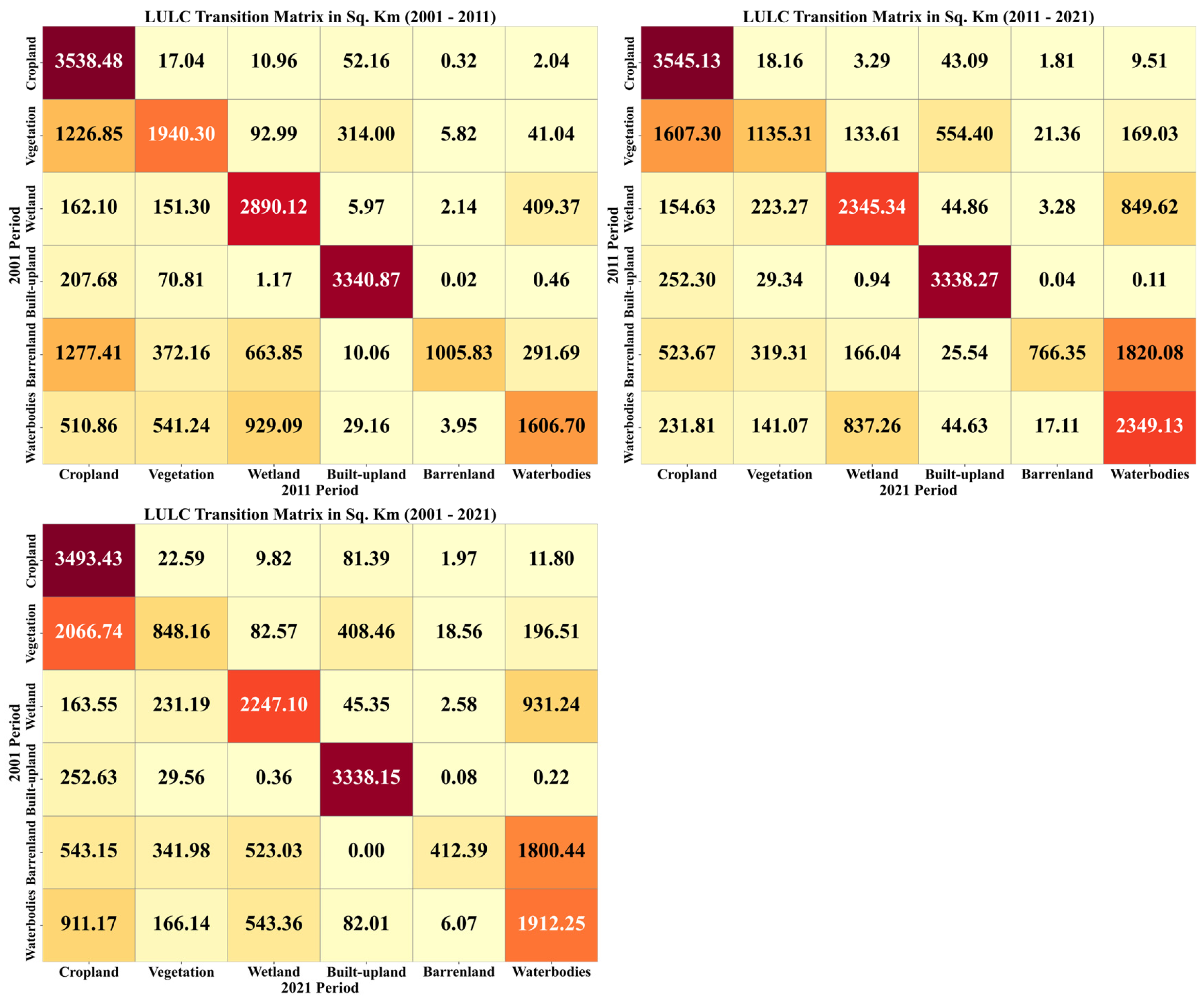
4.1.2. LULC Change Detection (2001–2021)

The study analyzed LULC changes from 2001 to 2021, revealing significant shifts. Cropland decreased by 1.14% during 2001–2011 and by 0.69% in 2011–2021. Vegetation declined slightly by 0.04% in the first period but saw a sharper drop of 0.37% in the second, linked to urban expansion. Wetland initially increased by 0.1% but decreased by 0.32%. Built-up areas grew by 1% during 2001–2011 and by 0.79% during 2011–2021. Barren land saw minor increases initially but rose significantly by 0.046% in the second period, possibly due to land abandonment. Water bodies expanded notably by 0.54% in 2011–2021, driven by artificial reservoirs and flooding. Urban growth and land degradation emerged as key concerns. The results of LULC changes (Δ) derived from transition statistics in CSV files generated using a pixel-based change detection method are detailed in

Table 4. LULC (Δ) change analysis (2001–2021) in km² and percentages.

LULC Classes	Area Change (km2 and %)
	2001–2011		2011–2021		2001–2021
	Δ Change		Δ Change		Δ Change
	km2	%	km2	%	km2	%
Cropland	−41.34	−1.14	−24.99	−0.69	−66.33	−1.83
Vegetation	−1.32	−0.04	−13.32	−0.37	−14.64	−0.40
Wetland	3.75	0.10	−11.60	−0.32	−7.85	−0.22
Built-up land	36.31	1.00	28.58	0.79	64.89	1.79
Barren land	0.19	0.01	1.65	0.05	1.84	0.05
Water bodies	2.41	0.07	19.68	0.54	22.09	0.61

, and the transition matrix is represented in Figure 7.

4.2. Urban Thermal Variations

4.2.1. Temporal Trends in LST

From 2001–2021, LST trends were analyzed using Landsat satellite imagery within the GEE platform. The results shown in Figure 8 revealed that in 2001, the highest temperature was observed to be 41 °C, while the LST rose by 2011 and was 42 °C, but by 2021, it dramatically increased, and the highest temperature was 55 °C, and the lowest was 26 °C. By 2011 and 2021, this heat intensity increased as many of these areas transformed from cropland, vegetation, and water bodies to built-up land. This significant rise in LST might be due to urbanization and the reduction in green spaces. However, this substantial growth in LST exhibited how swift urbanization affects the thermal environment [31,39,66].

4.2.2. UTFVI and Change Detection

The UTFVI, a measure of urban livability and thermal comfort, was analyzed for 2001, 2011, and 2021 to assess urban health and ecological quality. For the years 2001, 2011, and 2021, how the UTFVI was distributed throughout the study area is illustrated in Figure 9.

Historically, barren areas, wetlands, and paddy fields exhibited high UTFVI values, while central urban areas showed an increasing UTFVI over time. How each class of the UTFVI is distributed is detailed in Figure 10 in km² and percentages.

The “none” category decreased, representing optimal thermal comfort, reducing areas with ideal conditions. The “weak” and “middle” classes, reflecting moderate thermal conditions, increased from 1.72–5.01% and 1.73–4.96%, respectively. Conversely, the “strong” and “stronger” classes, denoting poor thermal comfort, expanded from 1.52–4.74% and 1.42–4.42%, respectively. The “strongest” class, representing extreme thermal stress, initially decreased from 30.58–26.36% (2001–2011) in 2011 but rebounded to 29.89% (2021). The detailed Δ changes in the UTFVI are detailed in

Table 5. UTFVI (Δ) changes analysis (2001–2021) in km² and percentages.

UTFVI Classes	2001–2011		2011–2021		2001–2021
	Δkm2	Δ%	Δkm2	Δ%	Δkm2	Δ%
None	−144.64	−4.00	−294.99	−8.15	−439.43	−12.13
Weak	89.43	2.47	29.78	0.82	119.22	3.29
Middle	79.67	2.20	40.62	1.12	120.29	3.32
Strong	68.81	1.90	47.70	1.32	116.53	3.22
Stronger	59.25	1.64	49.28	1.36	108.55	3.00
Strongest	−152.51	−4.21	127.61	3.53	−25.17	−0.69

.

Figure 11 presents the transformations in the UTFVI classes in km². The decline in optimal thermal zones and the rise in areas with extreme thermal stress suggest worsening urban livability, likely driven by urban expansion, reduced green cover, and increased impermeable surfaces, which exacerbate the urban heat island effect.

4.3. Future Projection of LULC and UTFVI Using the CA-ANN Model

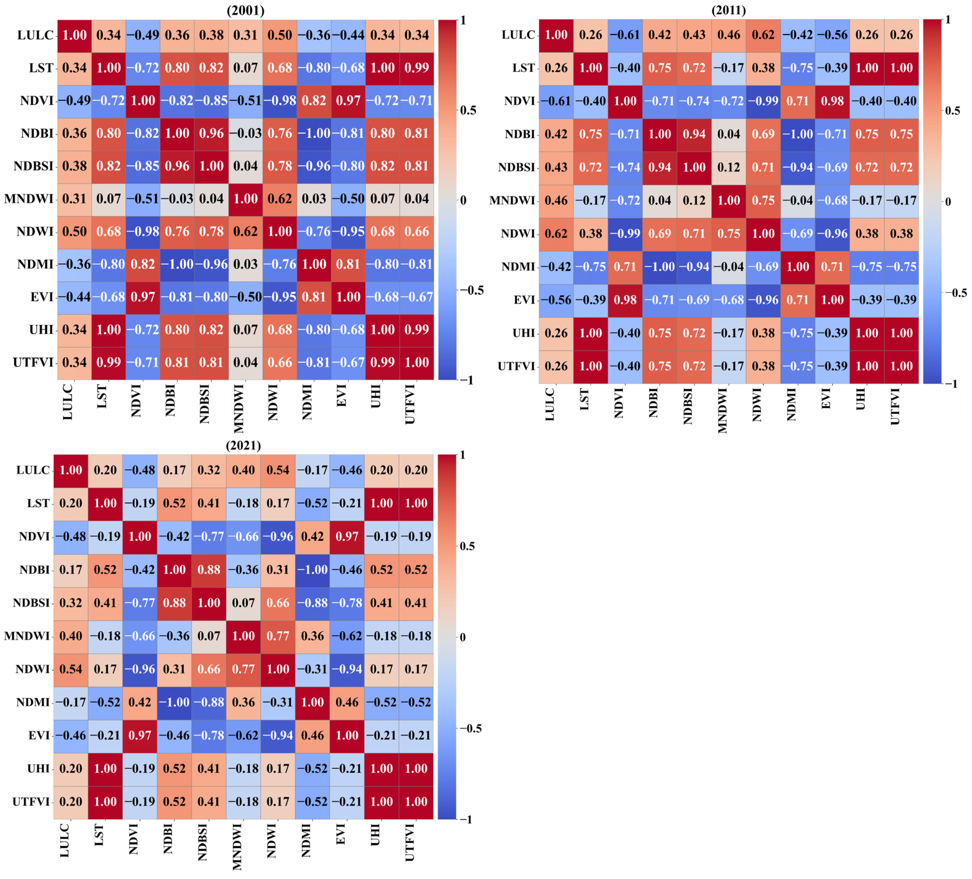
4.3.1. PCC Analysis

The analysis revealed significant relationships between EOIs, LULC, and thermal indices (LST, UHI, UTFVI) for 2001, 2011, and 2021. The findings are depicted as heat maps for each year in Figure 12. In 2001, LST showed strong positive correlations with the NDBI and NDBSI, indicating that built-up and bare soil areas contributed to higher temperatures, while negative correlations with the NDVI and EVI highlighted vegetation’s cooling effect. The UTFVI followed similar trends, linking urban expansion and reduced vegetation to increased thermal stress.

In 2011, LST maintained strong positive correlations with the NDBI and NDBSI, though its negative correlation with the NDVI weakened. The UTFVI continued to correlate strongly with LST and the NDBI, while the NDWI and MNDWI showed stronger links to LULC and the NDVI. By 2021, LST’s correlation with the NDBI and NDBSI weakened. The NDWI and MNDWI maintained strong correlations with the NDVI and LULC, underscoring the persistent cooling effects of water bodies and vegetation.

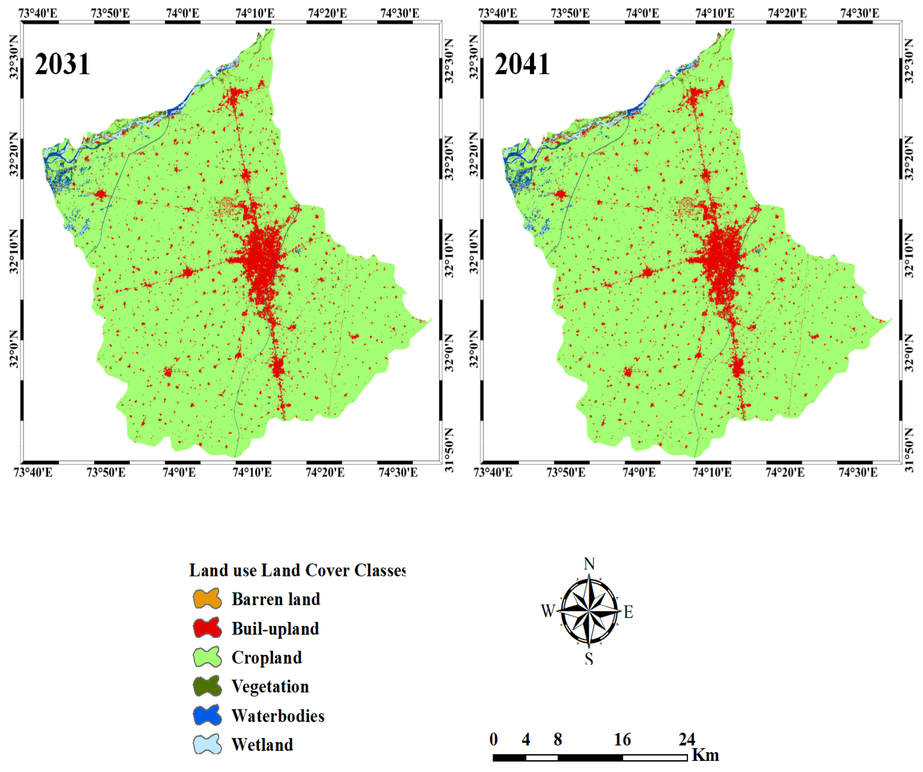
4.3.2. LULC Projection

The CA model simulations predict continued urbanization, with built-up land rising from 7.50–7.78% during 2021–2031 and 7.87% by 2041, primarily at the expense of cropland and vegetation. Cropland, though dominant, is predicted to decline marginally from 89.25–89.00% (2001–2031) and 89.10% (2041), as shown in

Table 6. Simulated LULC area distribution and (Δ) changes (2031–2041).

LULC Classes	2031				2041
	Area (km2)		%		Area (km2)		%
	km2 (2032)	Δ Changes (2021–2031)	% (2031)	Δ Changes (2021–2031)	km2 (2041)	Δ Changes (2031–2041)	% (2041)	Δ Changes (2031–2041)
Cropland	3223.51	−8.99	89.00	−0.25	3226.92	3.41	89.10	0.09
Vegetation	38.14	−0.42	1.05	−0.01	33.29	−4.86	0.92	−0.13
Wetland	37.04	−7.00	1.02	−0.19	33.32	−3.72	0.92	−0.10
Built-up land	281.70	9.98	7.78	0.28	285.03	3.33	7.87	0.09
Barren land	1.58	−0.58	0.04	−0.02	1.40	−0.18	0.04	−0.01
Water bodies	39.83	7.00	1.10	0.19	41.85	2.02	1.16	0.06

, reflecting cropland loss.

Vegetation and wetlands are expected to decline further. Vegetation declined from 1.06–1.05% (2021–2031) and 0.91% (2041), and wetlands from 1.22–1.02% (2021–2031) and 0.92% in 2041, likely due to urban encroachment. Water bodies may expand slightly, likely due to the conversion of wetlands or human activities like reservoir construction. Barren land may remain negligible, decreasing marginally by 2041. These projections, detailed in Table 6 and visualized in Figure 13, highlight persistent land use pressure and the need for sustainable planning to maintain balanced urban development and ecological preservation.

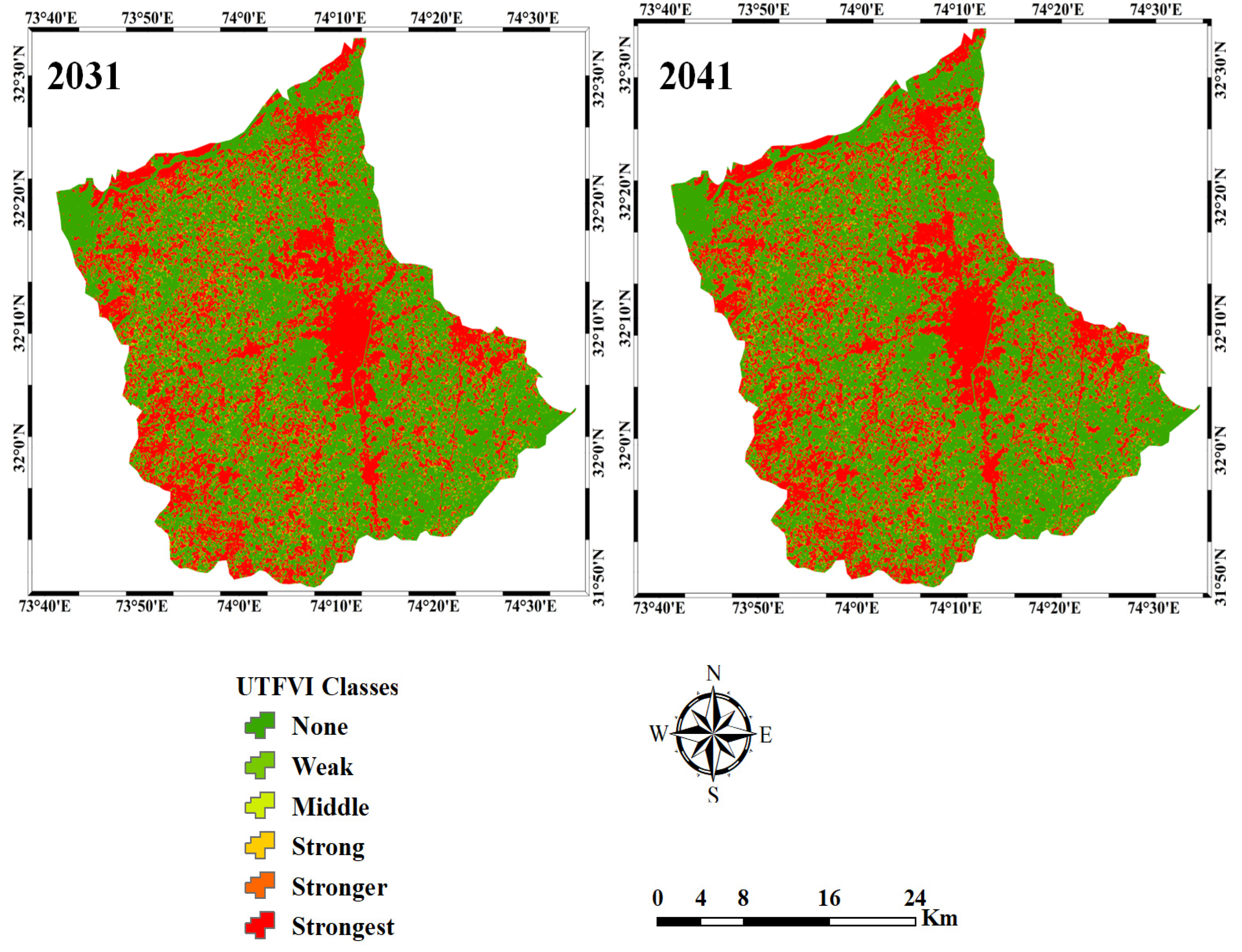
4.3.3. UTFVI Projection

The UTFVI simulation for 2031 and 2041, predicted using the ANN model, revealed significant trends in thermal variance, building upon historical patterns observed from 2001–2021.

The “none” category, denoting minimal thermal effects, is expected to slightly increase from 50.96–53.17% (2021–2031). However, there is a noticeable decline in the “none” category from 53.17–52.45% in 2041. The “weak” category is projected to decrease from 5.01–3.89% during 2021–2031 and 3.77% in 2041, while the “middle” category is expected to decline significantly from 4.95–2.54% in 2031, with a slight increase to 2.72% in 2041. The “strong” category is projected to decrease from 4.74–4.19% in 2031 and further to 3.79% in 2041.

The “stronger” category remains relatively stable, increasing slightly from 4.42–4.45% in 2031; however, it shifts to the “strongest” class in 2041, and the “strongest” class dramatically rises from 31.74–33.42% by 2041, indicating consistently high thermal variance in rapidly urbanizing regions. The projections (Figure 14,

Table 7. Simulated UTFVI area distribution and changes (2021–2041).

UTFVI Classes	2031				2041
	(km2)		%		(km2)		%
	km2 (2031)	Δ Changes (2021–2031)	% (2031)	Δ Changes (2021–2031)	km2 (2041)	Δ changes (2031–2041)	% (2041)	Δ Changes (2031–2041)
None	1925.73	80.01	53.17	2.21	1899.68	−22.94	52.45	−0.63
Weak	140.94	−40.51	3.89	−1.12	136.60	18.64	3.77	0.51
Middle	92.16	−87.22	2.54	−2.41	98.51	−16.39	2.72	−0.45
Strong	151.93	−19.78	4.19	−0.55	137.19	5.26	3.79	0.15
Stronger	161.34	1.33	4.45	0.04	139.46	−3.16	3.85	−0.09
Strongest	1149.69	66.16	31.74	1.83	1210.35	18.59	33.42	0.51

) highlight anomalies in thermal conditions, indicating the need for adaptive urban planning to mitigate heat risk.

4.4. UTFVI Variations Across Different LULC Classes

This analysis revealed how the UTFVI was distributed across various LULC categories between 2001 and 2021, with projections for 2031 and 2041 (Figure 15). This analysis highlights a significant trend in thermal variance, particularly in built-up areas, as well as in cropland. Cropland experienced a reduction in thermal resilience, with optimal (“none”) areas diminishing from 68.14% in 2001 to 53.93% in 2021, with projections showing a slight recovery to 56.43% in 2031 and 58.00% in 2041, suggesting some implementation strategies. Meanwhile, areas classified as the strongest rose by 25.40% in 2021, with a projected rise to 27.45% in 2031 and 28.50% in 2041. In contrast, vegetation showed improvement, with “none” areas tripling to 39.42% and projections indicating further increases to 39.56% in 2031 to 43.90% in 2041, while extreme heat conditions halved from 86.81 to 56.29%, with slight decreases projected to 55.66% in 2031 and 50.85% in 2041. Built-up land continued to serve as thermal hotspots, with over 85% categorized as “strongest” in 2021, decreasing slightly to around 83.45% in 2031 and 82.66% in 2041. Meanwhile, categories such as “stronger” and “strong” showed increasing trends, with “stronger” rising from 0.69% in 2001 to 4.38% in future projections to 2041, and “strong” rising from 0.67% to 1.70% over the same period. Notably, the proportions in the “none”, “weak”, and “middle” categories remained relatively low and stable, indicating persistent high thermal intensities in built-up areas despite some shifts towards less extreme categories in future projections. Wetlands face significant improvement, as “none” areas increased from 20.18% in 2001 to 75.99% in 2021, and future projections suggest a modest, slight decrease to 74.93% in 2031 and an increase again to 77.02% in 2041. Meanwhile, barren land and water bodies showed notable changes over the years. For barren land, “none” coverage increased significantly from 16.67% in 2001 to a peak of 91.88% in 2021. Still, projections indicate a decline to approximately 92.15% in 2031 and 64.72% in 2041, suggesting a substantial reduction in barren land by 2041. The “strongest” category for barren land decreased sharply from 78.06% in 2001 to 5.46% in 2021. Still, projections show a slight increase to 4.57% in 2031 and a rise again to 29.38% in 2041, implying a potential resurgence or redistribution of land types in future years. For water bodies, “none” coverage remained high, reaching 98.32% in 2021, with projections maintaining this high level at around 97.92% in 2031 and 97.81% in 2041, indicating stability. The “strongest” category for water bodies declined sharply from 29.38% in 2001 to 1.02% in 2021, with slight fluctuations projected in the future, remaining near 1%. Overall, the study revealed increasing UTFVI intensity, particularly in built-up areas and cropland, due to ongoing urbanization, as well as in cropland driven by changes in land management and agricultural practices. These trends highlight the urgency of heat-mitigation strategies like green infrastructure, cooling materials, and water-efficient farming practices.

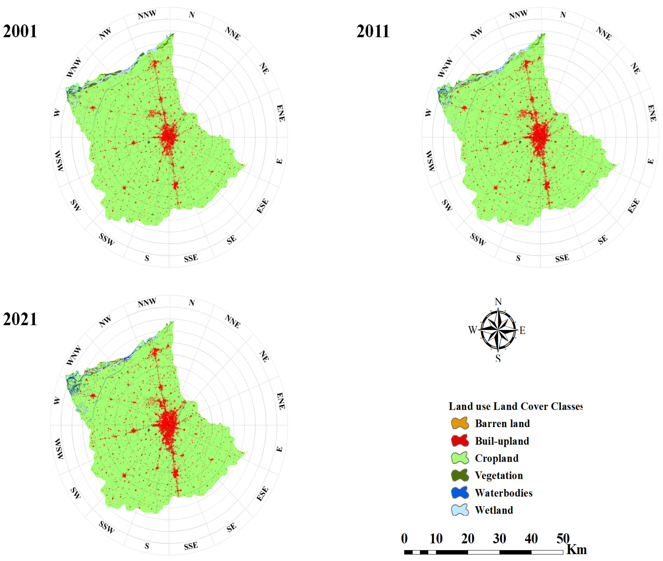
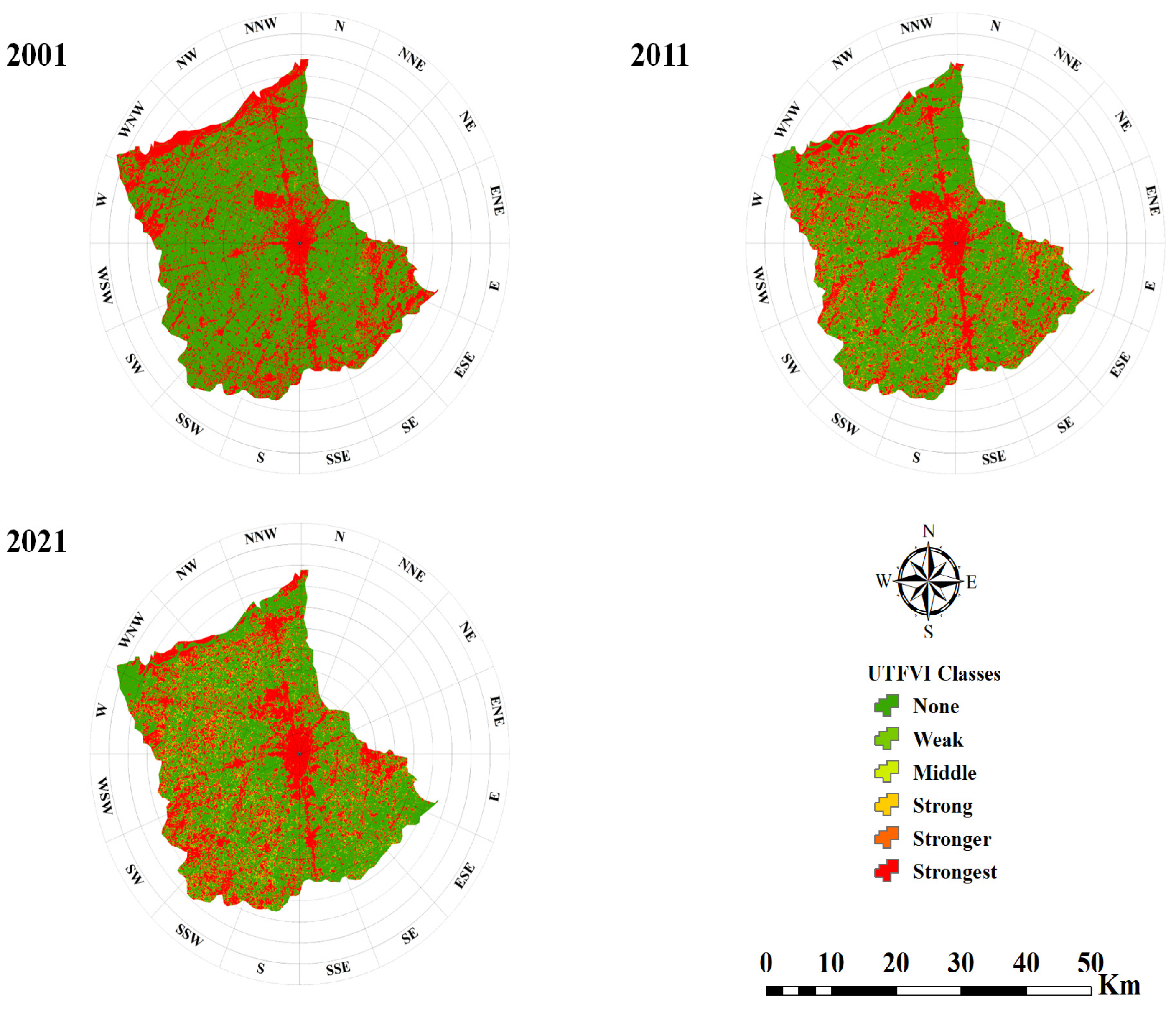
4.5. Directional Analysis of LULC and UTFVI

4.5.1. GDA of LULC (2001–2041)

The concentric rings analysis provides a detailed understanding of spatial and temporal shifts in LULC patterns (Figure 16). Cropland declined near the city center, especially in the east (E) and northeast (NE) directions, where cropland decreased from 63.19–56.01 km² in the east, but cropland remained dominant in the northwest (NW) and southeast (SE) directions. Projections (2031–2041) suggest accelerated cropland loss in the east, 56.01–55.29 km² due to urban encroachment.

Built-up land expanded significantly, particularly in the east and northeast directions, with built-up land increasing by 14.48–20.79 km² in the east and by 23.40–33.43 km² in the northeast. Projections indicate growth to 22.15 km² (E) and 35.62 km² (NE) by 2041, with annual expansion rates of 1.2% (E) and 1.5% (NE). The northern sector shows moderate growth, 11.33–13.24 km² by 2041, likely due to industrial development, infrastructure expansion, and population growth. Vegetation increased in the north by 0.49–1.00 km² but declined in the southwest by 0.10→0.07 km². Projections suggest northward expansion to 1.12 km² by 2041, while SW areas may fall further to 0.05 km², likely due to land conversion for urban or agricultural use. Wetlands grew in the northwest by 10.27–10.99 km² but shrank in the east by 0.25→0.15 km², with projections showing NW growth to 11.28 km² and E decline to 0.12 km² by 2041, indicating drainage or conversion for urban and agricultural purposes. Barren land nearly vanished in the northwest by 0.97–0.12 km², with projections indicating just 0.05 km² remaining by 2041. Water bodies remained stable in the north at 11.14–11.33 km² but declined in the west by 2.66–2.92 km² and are projected to decrease further to 2.85 km² by 2041, likely due to water extraction for agriculture or industry.

4.5.2. GDA of UTFVI (2001–2041)

The directional analysis of the UTFVI (Figure 17) provides a detailed understanding of urban heat distribution across specific directions from the city center, providing significant insights for urban planning and sustainability.

The “none” category declined markedly, particularly eastward from 2.24 to 1.78 km² and in the northeast from 0.82 to 0.70 km², reflecting reduced green spaces, with projections indicating further reductions by 2041: E: 1.03 km²; NE: 0.60 km². The “weak” class contracted in southern directions from 0.007 to 0.004 km², while “middle” intensity zones diminished west–northwest from 0.016 to 0.015 km², though 2041 projections show slight rebounds in “middle” zones: ESE: 0.064 km². Conversely, “strong” heat stress expanded northward from 0.020 to 0.023 km² and northeast from 0.050 to 0.061 km², with 2031–2041 data suggesting accelerated growth in eastern sectors from 0.131 to 0.124 km². The “stronger” category grew notably in eastern sectors from 0.033 to 0.082 km² and southeastern sectors from 0.034 to 0.159 km² and are projected to intensify by 2041: ESE: 0.168 km². Meanwhile, “strongest” intensities surged southward from 4.81 to 4.89 km² and southwest from 3.64 to 4.05 km², with 2041 peaks in southern corridors of 4.90 km². These trends (20–30%) decline in “none” and “weak” zones and (15–25%) rise in the “stronger” and “strongest” classes, highlighting escalating thermal stress, especially in eastern (E/ENE) and southern (S/SW) corridors, where projections suggest persistent amplification. Mitigation efforts should prioritize these high-risk areas through adaptive urban design and cooling interventions to counter both current and future heat extremes.

5. Discussion

This study comprehensively analyzes LULC changes, urban thermal dynamics, and their implications for sustainable development, contributing substantively to the global discourse on urbanization and environmental sustainability. By integrating advanced remote sensing techniques, statistical analyses, and predictive modeling, the research enhances the accuracy and reliability of LULC classification while offering actionable insights for policymakers and urban planners.

The findings reveal significant shifts in land use changes over the two decades. Moreover, LULC classification accuracy improved significantly, with overall accuracy rising from 85.27% (2001) to 92.36% (2021) and the kappa coefficient increasing from 0.86 to 0.93, reflecting enhanced model reliability. Cropland, built-up areas, and water bodies achieved high accuracy due to their distinct spectral characteristics, while wetlands and vegetation faced challenges due to spectral similarities, necessitating advanced techniques like LiDAR or hyperspectral imagery. These improvements are critical for reliable land use mapping and error identification [67], particularly in rapidly urbanizing regions where accurate data is essential for sustainable development.

The analysis of LULC changes reveals significant shifts driven by urbanization, with built-up areas expanding at the expense of cropland, wetlands, and vegetation. These trends are consistent with global patterns of urban growth fueled by socio-economic factors and rural-to-urban migration [4]. The decline in cropland raises concerns about food security, while the loss of wetlands and vegetation highlights ecological degradation. The growth of artificial water bodies reflects both intentional water management and climate-induced flooding. These findings emphasize the need for sustainable land use planning to balance urban growth with agricultural and ecological preservation, a challenge that resonates across rapidly developing regions worldwide [68].

The analysis reveals worsening urban heat conditions, with extreme thermal stress (“strongest” category) initially decreasing but rebounding to 29.89% by 2021. Urban planning dynamics, such as the expansion of low-density residential zones during the earlier period, reducing heat intensity, are followed by densification and commercial development in later years. The initial decline aligns with Punjab’s 2005–2010 environmental policies that relocated heat-intensive industries (e.g., steel, ceramics) from urban cores to designated industrial estates. Increased green spaces (parks, tree planting) helped cool urban areas [69,70]. This rebounding trend is driven by urban expansion, reduced green cover, an increase in production of relocated industries utilizing more coal, and increased impermeable surfaces, exacerbating the UHIE [17,71,72]. The decline in the “none” category and the expansion of the “strong” and “stronger” classes in urban areas, especially in industrial zones, underscores the need for innovative cooling strategies. Effective mitigation requires multi-pronged solutions, such as promoting green spaces, cool roofing technology, and efficient industrial improvements [73]. These measures are critical for addressing the adverse effects of UHIs, particularly in regions experiencing swift industrialization and urbanization.

The correlation analysis between LST and various indices reveals that built-up (NDBI) and bare soil areas (NDBSI) drive higher temperatures, while vegetation (NDVI, EVI) and water bodies exhibit cooling effects. The evolving urban thermal dynamics are evidenced by the weakening correlation between LST and built-up indices over time (2021), possibly due to the improved impact of improved urban design and green infrastructure [31]. These findings align with global efforts to promote energy-efficient urban design and enhance thermal regulation in cities facing rising temperatures.

Projections of future LULC changes indicate continued urban expansion, with built-up areas growing at the expense of cropland and vegetation. This trend, exacerbated by industrial demand for land, which drives land conversion and intensifies urban sprawl, poses significant risks to food security and rural economies. The decline in wetlands and vegetation further reflects the environmental impact of industrial activities and pollution on natural ecosystems. The expansion of water bodies, likely due to industrial water management practices such as reservoir construction, highlights the role of industrial cities in reshaping hydrological systems [17]. To address these challenges, sustainable urban planning strategies, such as mixed-use development, integrating green industrial zones, and circular economy principles, are essential for minimizing land use conflicts and environmental degradation.

Future scenarios indicate a rise in thermal stress (with the “strongest” category increasing by 2041), particularly in urban and suburban areas, driven by industrial growth and reduced green spaces. The shift toward extreme thermal effects is further exacerbated by the concentration of heat-intensive industries and transportation networks in urban peripheries [4]. These projections emphasize the importance of integrating blue–green infrastructure, promoting energy-efficient industrial practices, and adopting innovative cooling technologies to enhance urban livability and ecological resilience. Advanced urban planning strategies like creating green corridors, implementing reflective materials, and decentralizing renewable energy systems are essential to mitigate localized heat emissions and address the long-term impacts of urbanization [74].

The analysis of the UTFVI distribution across LULC categories from 2001 to 2021 reveals significant trends in thermal variance driven by urbanization and agricultural practices. Built-up areas consistently exhibited the highest thermal impact, highlighting the role of impervious surfaces and reduced green cover in intensifying UHI effects [75]. Cropland, particularly rice paddies, showed increasing thermal variance, suggesting that agricultural practices like continuous flooding in rice cultivation exacerbate thermal effects. Conversely, vegetation and wetlands demonstrated improvements, with the “none” category increasing and the “strongest” category declining, indicating that green cover and water management can mitigate thermal variance [4]. As the study area is a rice-growing city, cropland (especially rice paddies) significantly increases the UTFVI, suggesting that agricultural practices exacerbate thermal effects. There is a need for sustainable urban planning, including expanding green spaces, adopting the Alternate Wetting and Drying (AWD) method in rice cultivation, and incorporating water-sensitive designs to alleviate UHI effects.

The directional analysis of LULC changes in this study aligns with global patterns of urban expansion but reveals region-specific nuances. Like findings in Dhaka and Peshawar [4,33], built-up areas in our study grew most aggressively in the east and northeast, driven by infrastructure development and rural-to-urban migration. However, unlike Peshawar, where growth is radially uniform, our projections highlight directional disparities, with the northeast expanding faster than the east, likely due to topographic constraints absent in Peshawar’s plains. Cropland’s decline in the S/W mirrors trends observed in Peshawar, where urban sprawl consumed fertile peri-urban lands. Yet, our study uniquely notes the persistence of cropland dominance in the northwest, a contrast to Peshawar’s uniform agricultural loss. This divergence may reflect policy interventions. Vegetation increases in the north parallel urban greening successes in Dhaka, though our findings reveal a counter-trend in the southwest. Wetland expansion in the northwest contrasts with global declines, while eastward wetland loss echoes drainage for urbanization. These trends underscore the need for sustainable urban planning, including zoning regulations, greenbelt development, and agricultural land protection, to balance urban growth with ecological preservation and agricultural sustainability [4,33].

The directional analysis of UTFVI analysis reveals escalating thermal stress, particularly in southern and eastern sectors, aligning with global urban heat island patterns, while showing unique local variations. The 25% decline in “none” zones exceeds rates observed in comparable Asian cities [74], suggesting amplified impacts from industrial clustering and transport corridors. The “strongest” category’s expansion mirrors industrial cities like [17], but with the earlier emergence of “stronger” heat stress in southeastern areas. Key distinctions include the following: (1) faster thermal comfort loss in eastern sectors than radial cities, (2) persistent moderate-heat zones in northwestern areas, and (3) accelerated heat stress development near transport arteries. These findings reinforce the need for sector-specific cooling strategies, adapting successful approaches from Singapore to address our study area’s unique directional patterns [4].

6. Conclusions, Limitations, and Future Work

This study showed Gujranwala’s rapid urban expansion, driven by industrial growth and green space loss, while advancing prior research on LULC thermal dynamics in three key ways: (1) in our study, the RF classifier incorporating EOIs achieved a 92.36% overall accuracy (kappa = 0.93), outperforming conventional maximum likelihood methods [67], particularly for built-up areas (F1 score = 0.96) due to EOI-enhanced spectral separation; (2) the CA-ANN prediction model reliably projected LULC changes to 2031 and 2041 (kappa = 0.89, RMSE = 1.80, against 2021 data); and (3) unlike aggregate-scale analyses [4], 16-axis GDA revealed that industrial corridors—not just urban cores—drive extreme thermal stress, and rice paddies are identified as unexpected thermal contributors. The analysis of LST revealed a steady increase in urban temperatures, intensifying the UHI effect. The UTFVI analysis indicated that areas experiencing extreme heat conditions have grown, reflecting an increasing urban thermal burden. This trend underscores the growing impact of urbanization on the city’s microclimate, which may have significant implications for public health and environmental sustainability. Future projections suggest that expanding built-up areas will continue, leading to further vegetation and agricultural land reductions, likely to worsen the UHI effect. These findings are particularly relevant for industrial cities, where the dual pressures of urban expansion and industrial activities necessitate holistic approaches to land use and thermal management.

The limitations of this study include the following: (1) The 30 m resolution of Landsat provides robust regional-scale analysis of LULC patterns and thermal environments, but it may not capture sub-30 m urban features (e.g., individual buildings, narrow green spaces). (2) Additionally, the 20-year temporal scope may not fully capture long-term trends or sudden changes in urbanization and thermal dynamics. (3) This study focused on yearly analyses, which may overlook seasonal variations in thermal dynamics. (4) The study primarily relied on remote sensing data, with limited ground-based validation, which could affect the accuracy of the results. (5) The CA-ANN model contains uncertainties, particularly when forecasting future scenarios. (6) The classification of urban areas as a homogeneous “built-up land” category may overlook intra-urban heterogeneity in morphology (e.g., building density, green space distribution) and its thermal impacts. A more nuanced approach, such as Local Climate Zones (LCZs) or urban fraction zones, could better capture these variations.

Future studies could fuse Landsat with 10 m Sentinel-2 data to enhance feature resolution while retaining thermal analysis capabilities and integrating local climate data to improve the accuracy of thermal analyses. Seasonal data could be incorporated to better understand temporal fluctuations in thermal dynamics. Adopting the LCZ framework to classify urban areas by their structural and land cover characteristics (e.g., compact high-rises, low plants) enables targeted thermal mitigation strategies. Exploring advanced modeling techniques, such as deep learning models, could further enhance the accuracy of LULC and UTFVI predictions. Comparative studies in other industrial cities could help identify common patterns and unique challenges, while policy impact assessments could evaluate the effectiveness of proposed urban planning strategies. Integration of socio-economic, policy, and urban planning data in future studies could better unpack the mechanisms behind heat stress evolution. These insights advocate sustainable urban planning strategies incorporating green infrastructure and urban cooling measures to mitigate thermal stress.

References

1. Guo, A.; He, T.; Yue, W.; Xiao, W.; Yang, J.; Zhang, M.; Li, M. Contribution of Urban Trees in Reducing Land Surface Temperature: Evidence from China’s Major Cities. Int. J. Appl. Earth Obs. Geoinf. 2023, 125, 103570. [Google Scholar] [CrossRef]
2. Cui, J.; Ji, W.; Wang, P.; Zhu, M.; Liu, Y. Spatial–Temporal Changes in Land Use and Their Driving Forces in the Circum-Bohai Coastal Zone of China from 2000 to 2020. Remote Sens. 2023, 15, 2372. [Google Scholar] [CrossRef]
3. Talukdar, S.; Singha, P.; Mahato, S.; Shahfahad; Pal, S.; Liou, Y.-A.; Rahman, A. Land-Use Land-Cover Classification by Machine Learning Classifiers for Satellite Observations—A Review. Remote Sens. 2020, 12, 1135. [Google Scholar] [CrossRef]
4. Kafy, A.-A.; Saha, M.; Faisal, A.A.; Rahaman, Z.A.; Rahman, M.T.; Liu, D.; Fattah, M.A.; Al Rakib, A.; AlDousari, A.E.; Rahaman, S.N.; et al. Predicting the Impacts of Land Use/Land Cover Changes on Seasonal Urban Thermal Characteristics Using Machine Learning Algorithms. Build. Environ. 2022, 217, 109066. [Google Scholar] [CrossRef]
5. Ge, W.; Deng, L.; Wang, F.; Han, J. Quantifying the Contributions of Human Activities and Climate Change to Vegetation Net Primary Productivity Dynamics in China from 2001 to 2016. Sci. Total Environ. 2021, 773, 145648. [Google Scholar] [CrossRef]
6. Luo, Y.; Sun, W.; Yang, K.; Zhao, L. China Urbanization Process Induced Vegetation Degradation and Improvement in Recent 20 Years. Cities 2021, 114, 103207. [Google Scholar] [CrossRef]
7. Wang, Z.; Ishida, Y.; Mochida, A. Effective Factors for Reducing Land Surface Temperature in Each Local Climate Zone Built Type in Tokyo and Shanghai. Remote Sens. 2023, 15, 3840. [Google Scholar] [CrossRef]
8. Rasool, R.; Fayaz, A.; Shafiq, M.U.; Singh, H.; Ahmed, P. Land Use Land Cover Change in Kashmir Himalaya: Linking Remote Sensing with an Indicator Based DPSIR Approach. Ecol. Indic. 2021, 125, 107447. [Google Scholar] [CrossRef]
9. Miller, J.D.; Hutchins, M. The Impacts of Urbanisation and Climate Change on Urban Flooding and Urban Water Quality: A Review of the Evidence Concerning the United Kingdom. J. Hydrol. Reg. Stud. 2017, 12, 345–362. [Google Scholar] [CrossRef]
10. Stewart, K. Atmospheric Attunements. Environ. Plan. D 2011, 29, 445–453. [Google Scholar] [CrossRef]
11. Guo, A.; Yang, J.; Xiao, X.; Xia, J.; Jin, C.; Li, X. Influences of Urban Spatial Form on Urban Heat Island Effects at the Community Level in China. Sustain. Cities Soc. 2020, 53, 101972. [Google Scholar] [CrossRef]
12. Qian, Y.; Chakraborty, T.C.; Li, J.; Li, D.; He, C.; Sarangi, C.; Chen, F.; Yang, X.; Leung, L.R. Urbanization Impact on Regional Climate and Extreme Weather: Current Understanding, Uncertainties, and Future Research Directions. Adv. Atmos. Sci. 2022, 39, 819–860. [Google Scholar] [CrossRef]
13. Kazemi, A.; Cirella, G.T.; Hedayatiaghmashhadi, A.; Gili, M. Temporal-Spatial Distribution of Surface Urban Heat Island and Urban Pollution Island in an Industrial City: Seasonal Analysis. IEEE J. Sel. Top. Appl. Earth Obs. Remote Sens. 2025, 18, 7100–7116. [Google Scholar] [CrossRef]
14. Luo, Z.; Shao, Q.; Zuo, Q.; Cui, Y. Impact of Land Use and Urbanization on River Water Quality and Ecology in a Dam Dominated Basin. J. Hydrol. 2020, 584, 124655. [Google Scholar] [CrossRef]
15. Portela, C.I.; Massi, K.G.; Rodrigues, T.; Alcântara, E. Impact of Urban and Industrial Features on Land Surface Temperature: Evidences from Satellite Thermal Indices. Sustain. Cities Soc. 2020, 56, 102100. [Google Scholar] [CrossRef]
16. Soydan, O. Effects of Landscape Composition and Patterns on Land Surface Temperature: Urban Heat Island Case Study for Nigde, Turkey. Urban. Clim. 2020, 34, 100688. [Google Scholar] [CrossRef]
17. Liu, S.; Zhang, J.; Li, J.; Li, Y.; Zhang, J.; Wu, X. Simulating and Mitigating Extreme Urban Heat Island Effects in a Factory Area Based on Machine Learning. Build. Environ. 2021, 202, 108051. [Google Scholar] [CrossRef]
18. Chow, W.T.L.; Brennan, D.; Brazel, A.J. Urban Heat Island Research in Phoenix, Arizona: Theoretical Contributions and Policy Applications. Bull. Am. Meteorol. Soc. 2012, 93, 517–530. [Google Scholar] [CrossRef]
19. He, B.-J. Potentials of Meteorological Characteristics and Synoptic Conditions to Mitigate Urban Heat Island Effects. Urban. Clim. 2018, 24, 26–33. [Google Scholar] [CrossRef]
20. Halder, B.; Bandyopadhyay, J. Evaluating the Impact of Climate Change on Urban Environment Using Geospatial Technologies in the Planning Area of Bilaspur, India. Environ. Chall. 2021, 5, 100286. [Google Scholar] [CrossRef]
21. Shahfahad; Talukdar, S.; Rihan, M.; Hang, H.T.; Bhaskaran, S.; Rahman, A. Modelling Urban Heat Island (UHI) and Thermal Field Variation and Their Relationship with Land Use Indices over Delhi and Mumbai Metro Cities. Environ. Dev. Sustain. 2022, 24, 3762–3790. [Google Scholar] [CrossRef]
22. Venkatraman, S.; Kandasamy, V.; Rajalakshmi, J.; Sabarunisha Begum, S.; Sujatha, M. Assessment of Urban Heat Island Using Remote Sensing and Geospatial Application: A Case Study in Sao Paulo City, Brazil, South America. J. South. Am. Earth Sci. 2024, 134, 104763. [Google Scholar] [CrossRef]
23. Derdouri, A.; Wang, R.; Murayama, Y.; Osaragi, T. Understanding the Links between LULC Changes and SUHI in Cities: Insights from Two-Decadal Studies (2001–2020). Remote Sens. 2021, 13, 3654. [Google Scholar] [CrossRef]
24. Guha, S.; Govil, H. Annual Assessment on the Relationship between Land Surface Temperature and Six Remote Sensing Indices Using Landsat Data from 1988 to 2019. Geocarto Int. 2022, 37, 4292–4311. [Google Scholar] [CrossRef]
25. Mallick, S.K.; Rudra, S. Land Use Changes and Its Impact on Biophysical Environment: Study on a River Bank. Egypt. J. Remote Sens. Space Sci. 2021, 24, 1037–1049. [Google Scholar] [CrossRef]
26. Addas, A. Understanding the Relationship between Urban Biophysical Composition and Land Surface Temperature in a Hot Desert Megacity (Saudi Arabia). Int. J. Environ. Res. Public Health 2023, 20, 5025. [Google Scholar] [CrossRef]
27. Kumar Gavsker, K. Urban Growth, Changing Relationship between Biophysical Factors and Surface Thermal Characteristics: A Geospatial Analysis of Agra City, India. Sustain. Cities Soc. 2023, 94, 104542. [Google Scholar] [CrossRef]
28. Ali, M.B.; Jamal, S.; Ahmad, M.; Saqib, M. Unriddle the Complex Associations among Urban Green Cover, Built-up Index, and Surface Temperature Using Geospatial Approach: A Micro-Level Study of Kolkata Municipal Corporation for Sustainable City. Theor. Appl. Clim. 2024, 155, 4139–4160. [Google Scholar] [CrossRef]
29. Shamsudeen, M.; Padmanaban, R.; Cabral, P.; Morgado, P. Spatio-Temporal Analysis of the Impact of Landscape Changes on Vegetation and Land Surface Temperature over Tamil Nadu. Earth 2022, 3, 614–638. [Google Scholar] [CrossRef]
30. Jamei, Y.; Seyedmahmoudian, M.; Jamei, E.; Horan, B.; Mekhilef, S.; Stojcevski, A. Investigating the Relationship between Land Use/Land Cover Change and Land Surface Temperature Using Google Earth Engine; Case Study: Melbourne, Australia. Sustainability 2022, 14, 14868. [Google Scholar] [CrossRef]
31. Roy, B.; Bari, E. Examining the Relationship between Land Surface Temperature and Landscape Features Using Spectral Indices with Google Earth Engine. Heliyon 2022, 8, e10668. [Google Scholar] [CrossRef]
32. Mazhar, F.; Fadia, F. A Time Series Analysis of Satellite Imageries for Land Use & Land Cover (LULC) Change Detection of Gujranwala City, Pakistan from 1999–2019. Indian J. Sci. Technol. 2019, 12, 1–9. [Google Scholar] [CrossRef]
33. Khan, M.; Qasim, M.; Ahmad, A.; Tahir, A.A.; Farooqi, A. Predicting Land Use Dynamics, Surface Temperature and Urban Thermal Field Variance Index in Mild Cold Climate Urban Area of Pakistan. Heliyon 2024, 10, e38787. [Google Scholar] [CrossRef] [PubMed]
34. Mehmood, M.S.; Zafar, Z.; Sajjad, M.; Hussain, S.; Zhai, S.; Qin, Y. Time Series Analyses and Forecasting of Surface Urban Heat Island Intensity Using ARIMA Model in Punjab, Pakistan. Land 2023, 12, 142. [Google Scholar] [CrossRef]
35. Li, S.; Yang, X.; Cui, P.; Sun, Y.; Song, B. Machine-Learning-Algorithm-Based Prediction of Land Use/Land Cover and Land Surface Temperature Changes to Characterize the Surface Urban Heat Island Phenomena over Harbin, China. Land 2024, 13, 1164. [Google Scholar] [CrossRef]
36. Singgalen, Y.A. Spatio-Temporal Analysis through NDVI, NDBI, and SAVI Using Landsat 8/9 OLI. J. Comput. Syst. Inform. 2024, 5, 815–831. [Google Scholar] [CrossRef]
37. Dapke, P.P.; Nagare, S.M.; Quadri, S.A.; Bandal, S.B.; Gaikwad, R.M.; Baheti, M.R. Seasonal Analysis of Vegetation, Moisture, Urbanization, and Land Surface Temperature (LST) Using NDVI, NDMI, NDWI, and NDBI Indices: A Case Study of Sillod, Maharashtra. In Proceedings of the 2025 International Conference on Computational, Communication and Information Technology (ICCCIT), Indore, India, 7 February 2025; pp. 753–760. [Google Scholar]
38. Giachino, C.; Bollani, L.; Truant, E.; Bonadonna, A. Urban Area and Nature-Based Solution: Is This an Attractive Solution for Generation Z? Land Use Policy 2022, 112, 105828. [Google Scholar] [CrossRef]
39. Kafy, A.; MA, I.; Khan, M.H.H.; Sarker, M.H.S.; Rahman, M.W. Prediction of Future Land Surface Temperature and Its Impact on Climate Change: A Remote Sensing Based Approach In Chattogram City. In Proceedings of the 1st International Student Research Conference–2020, Dhaka, Bangladesh, 1 April 2020; pp. 1–12. [Google Scholar]
40. Uqaili Abdul, A.; Zafar, D.R.; Naeem, U.Z.; Bahrawar, J.; Muhammad, S.; Aisha, S.; Muhammad, S.; Shakeel, Q.; Fazal, A.S. Pakistan Statistical Year Book 2020; Pakistan Bureau of Statistics Govt of Pakistan: Islamabad, Pakistan, 2020; pp. 1–507.
41. Minallah, M.N.; Ghaffar, A.; Rafique, M.; Mohsin, M. Urban Growth and Socio-Economic Development in Gujranwala, Pakistan: A Geographical Analysis. Pak. J. Sci. 2016, 68, 176–183. [Google Scholar] [CrossRef]
42. Gondal, M.S.; Ayazuddin; Sandhu, A.J.; Awan, R. 7th Population & Housing Census “First Ever Digital Census” Key Findings Report The Largest Digitization Exercise of South Asia; Government of Pakistan, Ministry of Planning Development and Special Initiatives, Pakistan Bureau of Statistics, Statistics House: Islamabad, Pakistan, 2023.
43. Roy, D.P.; Wulder, M.A.; Loveland, T.R.; Woodcock, C.E.; Allen, R.G.; Anderson, M.C.; Helder, D.; Irons, J.R.; Johnson, D.M.; Kennedy, R.; et al. Landsat-8: Science and Product Vision for Terrestrial Global Change Research. Remote Sens. Environ. 2014, 145, 154–172. [Google Scholar] [CrossRef]
44. Phan, T.N.; Kuch, V.; Lehnert, L.W. Land Cover Classification Using Google Earth Engine and Random Forest Classifier—The Role of Image Composition. Remote Sens. 2020, 12, 2411. [Google Scholar] [CrossRef]
45. Xu, H. Modification of Normalised Difference Water Index (NDWI) to Enhance Open Water Features in Remotely Sensed Imagery. Int. J. Remote Sens. 2006, 27, 3025–3033. [Google Scholar] [CrossRef]
46. Rouse, J.W.; Haas, R.H.; Schell, J.A.; Deering, D.W. Monitoring the Vernal Advancement and Retrogradation (Green Wave Effect) of Natural Vegetation; NASA: Washington, DC, USA, 1973; pp. 1–120. [Google Scholar]
47. Huete, A.; Didan, K.; Miura, T.; Rodriguez, E.P.; Gao, X.; Ferreira, L.G. Overview of the Radiometric and Biophysical Performance of the MODIS Vegetation Indices. Remote Sens. Environ. 2002, 83, 195–213. [Google Scholar] [CrossRef]
48. Zha, Y.; Gao, J.; Ni, S. Use of Normalized Difference Built-up Index in Automatically Mapping Urban Areas from TM Imagery. Int. J. Remote Sens. 2003, 24, 583–594. [Google Scholar] [CrossRef]
49. Gao, B. NDWI—A Normalized Difference Water Index for Remote Sensing of Vegetation Liquid Water from Space. Remote Sens. Environ. 1996, 58, 257–266. [Google Scholar] [CrossRef]
50. McFeeters, S.K. The Use of the Normalized Difference Water Index (NDWI) in the Delineation of Open Water Features. Int. J. Remote Sens. 1996, 17, 1425–1432. [Google Scholar] [CrossRef]
51. Amini, S.; Saber, M.; Rabiei-Dastjerdi, H.; Homayouni, S. Urban Land Use and Land Cover Change Analysis Using Random Forest Classification of Landsat Time Series. Remote Sens. 2022, 14, 2654. [Google Scholar] [CrossRef]
52. Belgiu, M.; Drăguţ, L. Random Forest in Remote Sensing: A Review of Applications and Future Directions. ISPRS J. Photogramm. Remote Sens. 2016, 114, 24–31. [Google Scholar] [CrossRef]
53. Gorelick, N.; Hancher, M.; Dixon, M.; Ilyushchenko, S.; Thau, D.; Moore, R. Google Earth Engine: Planetary-Scale Geospatial Analysis for Everyone. Remote Sens. Environ. 2017, 202, 18–27. [Google Scholar] [CrossRef]
54. Papoutsis, I.; Bountos, N.I.; Zavras, A.; Michail, D.; Tryfonopoulos, C. Benchmarking and Scaling of Deep Learning Models for Land Cover Image Classification. ISPRS J. Photogramm. Remote Sens. 2023, 195, 250–268. [Google Scholar] [CrossRef]
55. Corcoran, J.; Knight, J.; Pelletier, K.; Rampi, L.; Wang, Y. The Effects of Point or Polygon Based Training Data on RandomForest Classification Accuracy of Wetlands. Remote Sens. 2015, 7, 4002–4025. [Google Scholar] [CrossRef]
56. Hu, J.; Liu, J.; Li, Z.; Zhu, J.; Wu, L.; Sun, Q.; Wu, W. Estimating Three-Dimensional Coseismic Deformations with the SM-VCE Method Based on Heterogeneous SAR Observations: Selection of Homogeneous Points and Analysis of Observation Combinations. Remote Sens. Environ. 2021, 255, 112298. [Google Scholar] [CrossRef]
57. Congalton, R.G.; Green, K. Assessing the Accuracy of Remotely Sensed Data; CRC Press: Boca Raton, FL, USA, 2019; ISBN 9780429052729. [Google Scholar]
58. Tewabe, D.; Fentahun, T. Assessing Land Use and Land Cover Change Detection Using Remote Sensing in the Lake Tana Basin, Northwest Ethiopia. Cogent Environ. Sci. 2020, 6, 1778998. [Google Scholar] [CrossRef]
59. Xiong, Y.; Xu, W.; Lu, N.; Huang, S.; Wu, C.; Wang, L.; Dai, F.; Kou, W. Assessment of Spatial–Temporal Changes of Ecological Environment Quality Based on RSEI and GEE: A Case Study in Erhai Lake Basin, Yunnan Province, China. Ecol. Indic. 2021, 125, 107518. [Google Scholar] [CrossRef]
60. Zhou, D.; Zhao, S.; Zhang, L.; Sun, G.; Liu, Y. The Footprint of Urban Heat Island Effect in China. Sci. Rep. 2015, 5, 11160. [Google Scholar] [CrossRef] [PubMed]
61. Weng, Q.; Lu, D.; Schubring, J. Estimation of Land Surface Temperature–Vegetation Abundance Relationship for Urban Heat Island Studies. Remote Sens. Environ. 2004, 89, 467–483. [Google Scholar] [CrossRef]
62. Sobrino, J.A.; Jiménez-Muñoz, J.C.; Paolini, L. Land Surface Temperature Retrieval from LANDSAT TM 5. Remote Sens. Environ. 2004, 90, 434–440. [Google Scholar] [CrossRef]
63. Avdan, U.; Jovanovska, G. Algorithm for Automated Mapping of Land Surface Temperature Using LANDSAT 8 Satellite Data. J. Sens. 2016, 2016, 1–8. [Google Scholar] [CrossRef]
64. Chen, J.; Zhan, W.; Du, P.; Li, L.; Li, J.; Liu, Z.; Huang, F.; Lai, J.; Xia, J. Seasonally Disparate Responses of Surface Thermal Environment to 2D/3D Urban Morphology. Build. Environ. 2022, 214, 108928. [Google Scholar] [CrossRef]
65. Liu, L.; Zhang, Y. Urban Heat Island Analysis Using the Landsat TM Data and ASTER Data: A Case Study in Hong Kong. Remote Sens. 2011, 3, 1535–1552. [Google Scholar] [CrossRef]
66. Pande, C.B.; Egbueri, J.C.; Costache, R.; Sidek, L.M.; Wang, Q.; Alshehri, F.; Din, N.M.; Gautam, V.K.; Chandra Pal, S. Predictive Modeling of Land Surface Temperature (LST) Based on Landsat-8 Satellite Data and Machine Learning Models for Sustainable Development. J. Clean. Prod. 2024, 444, 141035. [Google Scholar] [CrossRef]
67. Abu Yousuf, M.A.; Masrur, A.; Adnan, M.S.G.; Baky, M.A.A.; Hassan, Q.K.; Dewan, A. Spatio-Temporal Patterns of Land Use/Land Cover Change in the Heterogeneous Coastal Region of Bangladesh between 1990 and 2017. Remote Sens. 2019, 11, 790. [Google Scholar] [CrossRef]
68. Wang, A.; Zhang, M.; Ren, B.; Zhang, Y.; Al Kafy, A.-; Li, J. Ventilation Analysis of Urban Functional Zoning Based on Circuit Model in Guangzhou in Winter, China. Urban. Clim. 2023, 47, 101385. [Google Scholar] [CrossRef]
69. Khwaja, M.A. Environmental Challenges and Constraints to Policy Issues for Sustainable Industrial Development in Pakistan. 2012. Available online: https://d1wqtxts1xzle7.cloudfront.net/74392398/Environmental_Challenges_and_Constraints20211108-11027-o0169o.pdf?1738447655=&response-content-disposition=inline%3B+filename%3DEnvironmental_Challenges_and_Constraints.pdf&Expires=1752578623&Signature=cd-M~EVZB3pGLxdjNbsHHImxe31vGEYql4KflbMVXc~AaJg0YpJnsnAz8nXt92OD74KzWDXu2D0dZhjF6S28VxUpLkWp1OGqkNt4xgw7DCqmFaAYUXHej9-3kh3ohN4BC1jemeAKtVPOpHD~hLLVsslxNm1beK5Mx3szgffRTNdREAuaS1OnYxXcFirP0RbQnIYWpdH3aQpKYcXbkN~q99D9fx8VFDn549gumhhGhdDhuhoNTxeg7zdprLc53xoiLWhrPLgL21wowj-~BAO-1hKC2ZMfgYPTB8B0tFDk~rXnJIAHAkKk~YK46QFMANVdAzvjY7rYbvdgRoflLsyqQw__&Key-Pair-Id=APKAJLOHF5GGSLRBV4ZA (accessed on 10 November 2024).
70. Zahid, M.Y.; Qamar, M.K. The Aspects of Legislation in Environmental Management: Case Study of Punjab Province (Pakistan). Pak. J. Sci. 2020, 72, 138–153. [Google Scholar]
71. Kafy, A.-A.; Faisal, A.-A.; Al Rakib, A.; Fattah, M.A.; Rahaman, Z.A.; Sattar, G.S. Impact of Vegetation Cover Loss on Surface Temperature and Carbon Emission in a Fastest-Growing City, Cumilla, Bangladesh. Build. Environ. 2022, 208, 108573. [Google Scholar] [CrossRef]
72. Kafy, A.-A.; Faisal, A.A.; Rahman, M.S.; Islam, M.; Al Rakib, A.; Islam, M.A.; Khan, M.H.H.; Sikdar, M.S.; Sarker, M.H.S.; Mawa, J.; et al. Prediction of Seasonal Urban Thermal Field Variance Index Using Machine Learning Algorithms in Cumilla, Bangladesh. Sustain. Cities Soc. 2021, 64, 102542. [Google Scholar] [CrossRef]
73. Mathew, A.; Arunab, K.S.; Kumar Sharma, A. Revealing the Urban Heat Island: Investigating Spatiotemporal Surface Temperature Dynamics, Modeling, and Interactions with Controllable and Non-Controllable Factors. Remote Sens. Appl. 2024, 35, 101219. [Google Scholar] [CrossRef]
74. Zhang, M.; Tan, S.; Zhang, Y.; He, J.; Ni, Q. Does Land Transfer Promote the Development of New-Type Urbanization? New Evidence from Urban Agglomerations in the Middle Reaches of the Yangtze River. Ecol. Indic. 2022, 136, 108705. [Google Scholar] [CrossRef]
75. Chen, Y.; Yang, J.; Yang, R.; Xiao, X.; Xia, J. Contribution of Urban Functional Zones to the Spatial Distribution of Urban Thermal Environment. Build. Environ. 2022, 216, 109000. [Google Scholar] [CrossRef]
Figure 1. Study area map, Gujranwala, Punjab, Pakistan.
Remotesensing 17 02474 g001
Figure 2. Methodological flowchart for the study.
Remotesensing 17 02474 g002
Figure 3. Confusion matrix for LULC classification accuracy (2001–2021).
Remotesensing 17 02474 g003
Figure 4. Accuracy metrics for LULC classification (2001–2021).
Remotesensing 17 02474 g004
Figure 5. LULC classification maps for the years 2001, 2011, and 2021.
Remotesensing 17 02474 g005
Figure 6. Area distribution of LULC classes (2001–2041) in km2 and percentages.
Remotesensing 17 02474 g006
Figure 7. LULC transition matrix (2001–2021) in km2..
Remotesensing 17 02474 g007
Figure 8. LST variations (2001–2021).
Remotesensing 17 02474 g008
Figure 9. UTFVI maps (2001–2021).
Remotesensing 17 02474 g009
Figure 10. UTFVI class distribution (2001–2021) in km2 and percentages.
Remotesensing 17 02474 g010
Figure 11. UTFVI class transformations (2001–2021).
Remotesensing 17 02474 g011
Figure 12. PCC heatmaps for EOIs, LULC, and thermal indices (2001–2021).
Remotesensing 17 02474 g012
Figure 13. Simulated LULC maps for 2031 and 2041.
Remotesensing 17 02474 g013
Figure 14. Simulated UTFVI maps for 2031 and 2041.
Remotesensing 17 02474 g014
Figure 15. UTFVI distribution across LULC classes (2001–2021).
Remotesensing 17 02474 g015
Figure 16. GDA maps of LULC changes (2001–2021).
Remotesensing 17 02474 g016
Figure 17. GDA maps of UTFVI changes (2001–2021).
Remotesensing 17 02474 g017