A Multi-Receiver GNSS System Geometry Control Algorithm in Mobile Measurement of Railway Track Axis Position

Abstract

Accurate diagnostics of the railway track axis are crucial for enabling higher operational speeds of rail vehicles. Consequently, assessment methods are under continuous refinement. The precision of mobile GNSS-based measurements is influenced by external factors such as terrain obstructions and satellite geometry. This study presents an innovative approach that continuously monitors a predefined multi-receiver GNSS configuration in real time to enhance positioning accuracy. Field experiments on operational railway lines demonstrate that the proposed method significantly improves measurement reliability and reduces uncertainty compared to the conventional CQ-based quality assessment. The algorithm underlying the proposed method is formulated through analytical equations, allowing it to be implemented in any programming environment. The method’s effectiveness is demonstrated by comparing the expanded uncertainty calculated using GNSS-provided data with that obtained through the proposed approach.

1. Introduction

The geometric layout of a railway track axis plays a crucial role in enabling higher permissible speeds for rail vehicles. To ensure safety and performance, the designed alignment must be precisely staked out in the field, with actual parameters closely matching the design specifications. An additional challenge arises when the track axis must be identified based on an existing railway line, particularly during modernization projects where the new alignment is derived from evaluating the current condition of the track. This situation is common when upgrading existing lines to improve operational parameters.

Often, modernized tracks lack an accurate digital model of their geometry, necessitating the inventory of horizontal and vertical coordinates of the track. For this data to support reliable identification of geometric parameters, it must be obtained through precise, accurate, and quasi-continuous measurements. Traditionally, this is accomplished using geodetic methods based on high-precision tacheometry, where surveying instruments refer to a stable geodetic control network established along the railway line. However, such measurements are both time-consuming and costly, especially when applied across extensive railway corridors [1,2,3,4]. Tacheometric measurement methods have a long-standing tradition and, despite ongoing innovations, remain labor-intensive and require the involvement of multiple personnel. Nonetheless, they provide measurements characterized by low uncertainty and high precision.

A second category of techniques for determining the position and geometry of the track axis consists of mobile measurement methods, primarily based on Global Navigation Satellite System (GNSS) technologies combined with inertial measurement units (IMUs) [5,6,7,8,9]. These methods offer significantly greater efficiency due to the higher speeds that can be achieved by measurement platforms. However, the uncertainty of the resulting track axis coordinates depends on numerous factors, including the current satellite constellation configuration—an inherently variable parameter—and local terrain conditions such as vegetation, buildings, and other obstructions, which are relatively fixed. Additionally, these measurements require a methodology that accounts for the spatial offset between the GNSS antennas or IMU sensors and the actual track axis, as direct placement of sensors on the track axis is typically infeasible [10].

Currently, the uncertainty of GNSS-based measurements is typically evaluated using quality coefficients: CQ2D for horizontal positioning and CQ3D for three-dimensional positioning, each assigned to individual measurements [11]. This approach is particularly appropriate in the context of static measurements, where long time series consisting of tens of thousands of individual position recordings are collected. Through statistical analysis of such datasets, measurements with CQ values exceeding predefined thresholds can be identified and excluded [12]. Provided that the proportion of these outliers within the dataset is small, their impact on the overall measurement result remains negligible.

In the case of mobile measurements, however, each recorded position must be treated as a single, non-repetitive observation. Consequently, assessing uncertainty solely based on CQ quality indicators is insufficient. These coefficients represent the standard deviation, indicating the probability that the true measurement value (i.e., the coordinates) lies within the spatial region defined by the CQ value [12].

Therefore, it is possible that the true value deviates only slightly from the indicated measurement, even when the CQ coefficient suggests high uncertainty. According to traditional GNSS positioning analysis methods, such samples would be discarded for failing to meet accuracy requirements, despite potentially being usable in practice [13]. This conservative approach may result in overly strict evaluation criteria, rendering measurements in challenging environments—such as areas with significant terrain obstructions—difficult or nearly impossible to conduct.

Moreover, practical experience demonstrates the opposite scenario: a measurement with a relatively low CQ value may exhibit a significant deviation from the receiver’s true position. In such instances, an erroneous estimation of the track axis position could be mistakenly accepted as valid.

This article presents an innovative method for evaluating recorded railway track axis positions obtained from a mobile rail-based measurement platform [13,14,15]. The proposed approach relies on continuous monitoring of the geometric configuration of a multi-receiver GNSS measurement system, enabling a reduction in measurement uncertainty and enhancing the reliability of GNSS-based railway track axis positioning.

By applying this approach, an acceptable level of measurement precision can be achieved even in challenging terrain conditions that limit satellite signal availability. Theoretical considerations and the developed method were tested on measurement data collected during field experiments on operational railway lines. The resulting uncertainties of the measured track axis positions were then compared with conventional CQ quality indicators.

In the field of inventory and maintenance measurements using GNSSs, a significant problem is the conditions (especially terrain conditions generating apertures on the satellite-receiver path), which affect the quality of position determination. The process of identifying the defined receivers’ geometric frame on railway lines is particularly affected by this problem due to the fact that it runs through a terrain that is diversified in terms of the immediate surroundings and due to the need to achieve high positioning accuracy. In order to ensure the required quality of measurement signals, a number of methods have been developed in which techniques such as RAIM (Receiver Autonomous Integrity Monitoring), ML (machine learning) or DF (Data Fusion) are implemented [16,17,18].

This paper presents a certain narrow approach using analytical processing of data from a multi-antenna measurement system, which uses geometrical relations of the GNSS receiver antenna system. The computational algorithm uses criteria and conditions related to the assessment of the uncertainty of individual positions. The advantage of this approach is that it includes a clearly defined set of equations in an analytical form—the solutions are exact and reliably guarantee the speed of calculations on arbitrarily large datasets and a relatively simple implementation—which makes this approach practical. The effectiveness of the method was presented on the CQ2D indicator, which is commonly used in RTK measurements and in the analysis of the reliability of GNSS measurements. It should be emphasized, however, that referring to other uncertainty measures (e.g., RMSH and RMSV) does not affect the structure of the computational algorithm, but may change the percentage of line sections in which the aforementioned position uncertainty is effectively reduced. Therefore, the presented algorithm is not particularly related to any uncertainty measure used in the RTK technique. As part of future research, the authors intend to assess the reduction in uncertainty using other measures provided by RTK/RTN services.

The research presented in this article was conducted within the framework of the InnoSatTrack research project, which aimed to develop a set of methods for efficient, relatively fast, and sufficiently accurate mapping of the railway track axis into a geometric layout. The software system developed as part of the project supports this functionality; however, precise identification of geometric parameters—expressed in the form of a curvature diagram—requires a relatively dense distribution of track axis positions, preferably with minimal data gaps. This article focuses on an algorithm designed to enhance the capabilities of the applications developed within the project.

The measurement methodology using an instrumented platform wagon was developed in accordance with the procedures established by the national railway infrastructure manager. The measurement platform wagon run described herein was conducted as part of a scheduled train movement listed in the PKP PLK timetable. All field activities carried out by the authors were performed under the direct supervision of the personnel of the Railway Line Department.

2. Materials and Methods

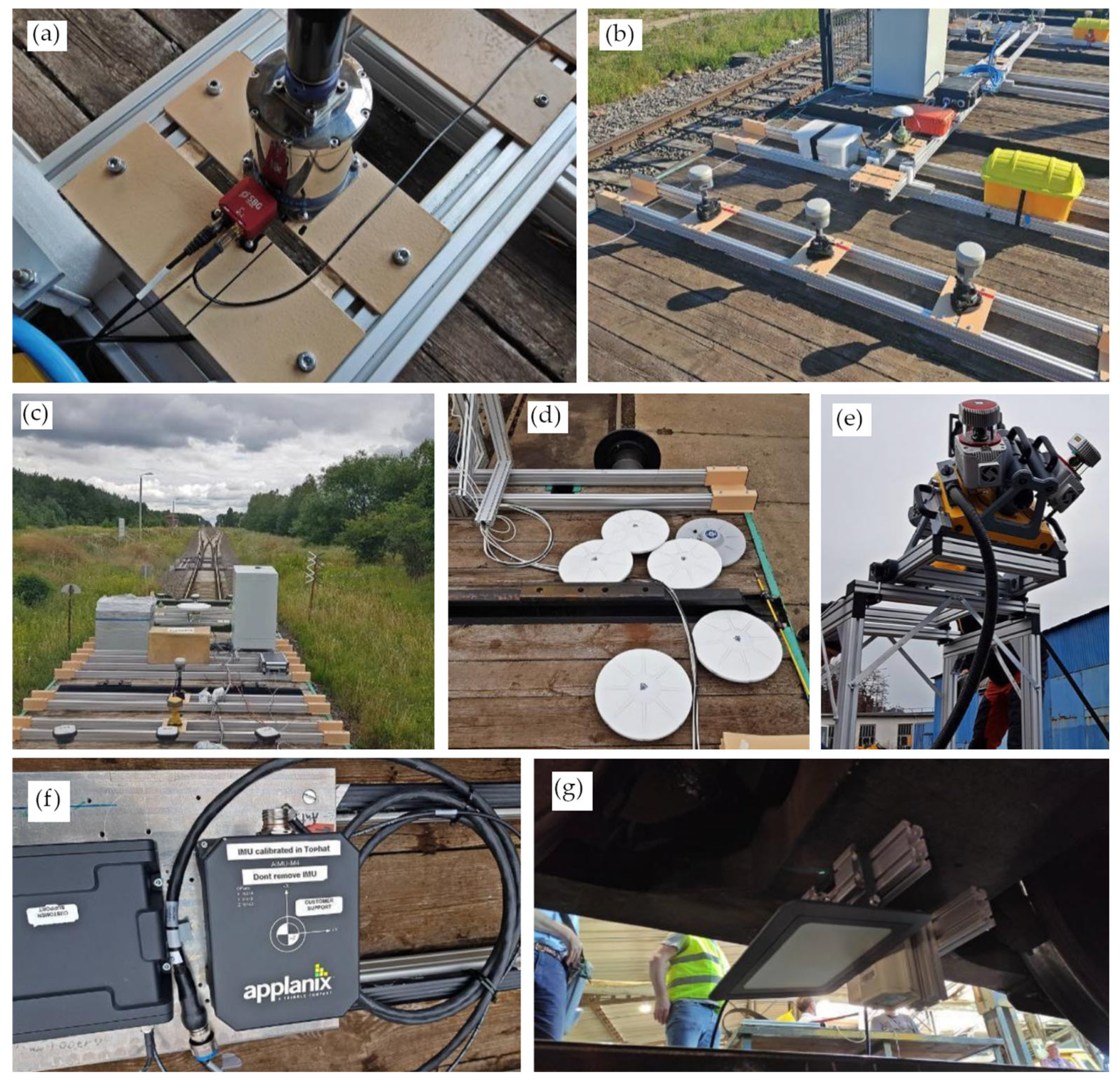
2.1. Mobile Satellite-Based Measurement of the Track Axis

This article focuses on a measurement method developed by the authors for determining the position and geometry of the railway track axis within a designated spatial reference frame, typically the officially adopted one [19]. To achieve this, the authors designed an integrated measurement and information system (illustrated in Figure 1) that leverages advanced GNSS (Global Navigation Satellite System) positioning techniques (Figure 1b–d), supported by an Inertial Navigation System (INS) (Figure 1a,f), photogrammetry (Figure 1g), and Terrestrial Laser Scanning (TLS) methods (Figure 1e). The measuring equipment was selected by the authors based on its commercial availability, ensuring that access to the necessary hardware would not impede future implementation, while maintaining a high-standard metrological performance.

Each of these techniques plays a crucial role in addressing the diverse conditions encountered during continuous mobile measurements. The data recorded by each system are time-synchronized, ensuring their contributions are properly aligned during processing to enhance measurement reliability and reduce uncertainty.

The GNSS is central to the proposed solution, thanks to advances in RTK/RTN (Real-Time Kinematic/Real-Time Network) technologies, which apply real-time corrections to raw measurements and yield position accuracies on the order of a few centimeters. However, continuous GNSS-based measurements must be supplemented by the INS, which provides platform tilt angles—both longitudinal slopes due to track gradients and transverse tilts from track irregularities or superelevation on curves.

The INS further enhances the measurement process in situations where terrain obstructions severely degrade satellite signal reception. Photogrammetric techniques were used to compute corrections for minor wheelset displacements relative to the rail heads, which arise from the vehicle’s dynamic behavior—such as yaw motions and curve negotiation. Terrestrial Laser Scanning (TLS) provides an alternative and complementary source of spatial information, which is particularly valuable during prolonged GNSS signal loss, such as in sections where even INS data must be spatially corrected [20].

2.2. Determination of the Track Axis and Measurement Uncertainty

The track axis is a theoretical line on the track surface, positioned midway between the rail heads (or, on horizontal curves, referenced to the outer rail) along the track’s longitudinal direction. As a designed element, its characteristics directly influence operational parameters—most notably the permissible train speeds. As discussed in Section 1, determining the actual spatial geometry of the track axis within a coordinate system is essential for assessing existing railway lines. The measurements conducted by the authors supply the required data to compute both the track axis coordinates and their associated uncertainties.

The measurement method fundamentally relies on synchronous satellite observations acquired by GNSS receivers [10,15]. Receiver positions are computed in the WGS-84 reference frame using known satellite ephemerides and measured pseudoranges [11], a process known as spatial trilateration. Cartesian Earth-Centered Earth-Fixed (ECEF) coordinates and the receiver clock bias are iteratively estimated via least-squares adjustment. These ECEF coordinates (x, y, z) are then transformed into curvilinear coordinates—latitude, longitude, and ellipsoidal height (B, L, h) [21]. Ellipsoidal heights are further corrected using a discrete geoid or quasi-geoid model to yield orthometric or normal heights, which reference the mean sea level [22,23]. The choice of vertical reference system is governed by national legislation; in Poland, the EUVN2007 normal height system, tied to the Amsterdam tide gauge, is employed [24].

Three-dimensional ellipsoidal coordinates must be projected into planar map coordinates to facilitate the computation of linear and angular measurements, as well as areas. Among the various cartographic projections employed in geodesy, navigation, hydrography, and military applications, Gauss–Krüger projection—known in English as the Transverse Mercator projection—is widely used for its conformality and minimal distance distortions [25,26].

In this method, the convex surface of a segment of the Earth’s rotational ellipsoid is mapped onto narrow meridian zones, which are typically 3° or 6° wide. A selected zone segment, representing the area of interest, is then used for detailed mapping. In the classical Gauss–Krüger projection, only the central meridian is free of linear distortion; distortion increases progressively toward the zone boundaries. To optimize distortion distribution, a scale factor is applied within each meridian zone [27,28].

For instance, the PL-2000 coordinate system—used for railway measurements in Poland—employs a 3° meridian zone with a scale factor of 0.999923. This results in linear distortions of approximately −7.7 cm/km on the central meridian and +7.0 cm/km at the zone edges. Consequently, lines of zero distortion are shifted east and west of the central meridian, occurring at two specific longitudes. This adjustment produces a more uniform distortion distribution, which is crucial for national geodesy and spatial planning. Coordinates in the PL-2000 system are expressed as northings (X) and eastings (Y) [19].

Synchronous satellite measurements from six receivers mounted on the platform are processed either in real time using RTK/RTN corrections or during post-processing with precise SP3 orbit data [11]. In both modes, each receiver’s instantaneous position is reported alongside a parameter quantifying its accuracy. First, the partial derivative matrix of the GNSS observation equations is used in a least-squares adjustment to compute the variance–covariance matrix [29]. Its diagonal entries represent the variances of the adjusted estimators for the ECEF coordinates and the receiver clock bias. After transforming these ECEF coordinates into the local east–north–up (ENU) frame, a rotation matrix is applied to update the variance–covariance matrix, from which the DOP coefficients—HDOP (horizontal), VDOP (vertical), and PDOP (positional)—are derived [30]. Finally, these DOP values are converted into the CQ quality indicators: CQ2D for horizontal position, CQ1D for vertical position, and CQ3D for three-dimensional positioning errors [31].

Trimble R10 GNSS receivers were used to collect the data for the study. The receiver-transmitted satellite data and received RTK/RTN correctional data were processed jointly in the Trimble Access software of the receiver controller. To estimate the single-point error, despite the Dilution-Of-Precision (DOP) coefficients, the signal analysis and filtering were performed by the software. The quality check of the calculated data included the issue of elimination of potentially erroneous satellite signals. A sample measurement record is presented in

Table 1. Sample record of GNSS RTK/RTN measurement.

Parameter	Value
Point Id	5830F00170_20210609_083941749
Start Time	9 June 2021 08:39:42
GPS Time	2161 290381.750
WGS84 Cartesian X [m]	3,531,069.0187
WGS84 Cartesian Y [m]	1,191,245.5035
WGS84 Cartesian Z [m]	5,158,894.6301
WGS84 Latitude [°]	54.33952279°N
WGS84 Longitude [°]	18.64239643°E
WGS84 Ellip. Height [m]	34.6315
Easting [m]	6,541,778.6156
Northing [m]	6,023,434.1565
Ortho. Height [m]	5.3597
CQ 3D [m]	0.0112
CQ 2D [m]	0.0063
CQ 1D [m]	0.0092
PDOP	2.1
HDOP	1.2
VDOP	1.7
GDOP	2.9
GPS SVs	6/9
GLONASS SVs	4/5
Galileo SVs	-
Beidou SVs	-

.

The receiver software used in the described position calculated only part of all receiver satellite signals: 6 satellites out of 8 for GPS system (GPS SVs) and 4 out of 5 of the GLONASS system (GLONASS SVs). Hence, the obtained CQ values include the important issue of elimination of false observations.

Independent and reliable ground truth data for the analyzed railway track axis were not available. Typically, the coordinates of points describing the railway axis in Poland are obtained through tachymetric measurements, which rely on the national geodetic control network. Given the length of the analyzed track section, these measurements were based on control points from multiple geodetic traverses. As a result, the adjusted coordinates of the control points may have been affected by errors ranging from a few millimeters to several centimeters. This implies that, despite using a consistent reference frame (PL-2000), significant discrepancies may arise in large-scale analyses, such as the one presented in this study.

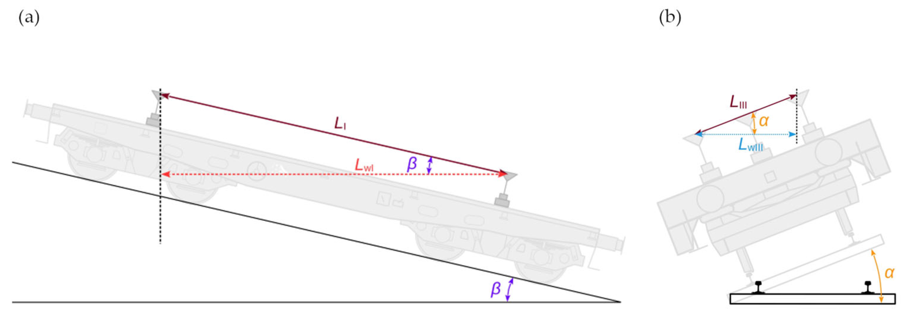
2.3. Measurement Platform Configuration and Correction Principle

To evaluate the potential for uncertainty reduction and reliability enhancement in a mobile railway track axis positioning system, a six-antenna, multi-receiver configuration was implemented on the measurement platform. Two primary antennas were mounted directly above the bogie pivot points, while four auxiliary antennas were arranged at known offsets to form a rectangular array (Figure 2). Synchronous GNSS measurements from this array of six receivers, each with precisely surveyed horizontal offsets, provide redundant observations that improve the accuracy of the pivot-point antenna positions.

Antennas AC and BC, which are mounted directly above the bogie pivots (Figure 2a), serve as the primary receivers, while the remaining four act as auxiliary receivers. Antenna positioning was performed with tachymetric precision: longitudinal beams affixed to the platform supported specialized mounts featuring holes for the centering screws of geodetic prisms. Prior to antenna installation, prism locations were measured with a tachymeter using reference prisms. Following adjustment, the antenna array achieved a precisely surveyed spatial configuration, with coordinate uncertainty below 1 mm.

The proposed method employs an analytical solution to correct the coordinates of the primary receivers mounted above the bogie pivots. To simplify the correction algorithm, the actual antenna positions are constrained to an ideal rectangular layout (Figure 2b), reducing the number of parameters required for computing the X and Y adjustments. The pairwise distances between antennas are then represented in a symmetric distance matrix L, as defined by Equation (1):

$$\mathit{L}=\left[\begin{array}{ccc}0& \cdots & L_{ij}\\ ⋮& \ddots & ⋮\\ L_{ij}& \cdots & 0\end{array}\right],i=\mathrm{1,2},\cdots ,6 j=\mathrm{1,2},\cdots ,6$$

(1)

where $\mathit{L}=\sqrt{{\left(X_i-X_j\right)}^2+{\left(Y_i-Y_j\right)}^2}$.

$X_i,Y_i$—coordinates of the prism mounted on the mounts during the tachymetric adjustment of the antenna positions on the platform.

The determined control distances can be divided into so-called “short” distances, corresponding to the transverse dimensions (L₄–L₉), and “long” distances characteristic of the longitudinal dimensions (L₁–L₃) and (L₁₀–L₁₅) (cf. Figure 3). Using the notation from Figure 3a, we obtain the matrix L, which is a symmetric matrix, and the rectangular layout in which the antennas are arranged leads to a reduction in the values of individual lengths, which can be grouped as follows:

$$L_1=L_2=L_3=L_{\mathrm{I}}$$

(2)

$$L_4=L_5=L_6=L_7=L_{\mathrm{I}\mathrm{I}}$$

(3)

$$L_8=L_9=L_{\mathrm{I}\mathrm{I}\mathrm{I}}$$

(4)

Taking into account the track’s inclination, the distances between the GNSS receivers determined in two-dimensional Euclidean space require adjustment for their reduction. This is illustrated in Figure 3. In such a case, the reference distance values will be as follows:

• For L₁, L₂ and L₃:

$$L_{\mathrm{w}\mathrm{I}}=L_{\mathrm{I}}·\cos \beta$$

(5)

For L₄, L₅, L₆ and L₇:

$$L_{\mathrm{w}\mathrm{I}\mathrm{I}}=L_{\mathrm{I}\mathrm{I}}·\cos \alpha$$

(6)

For L₈ and L₉:

$$L_{\mathrm{w}\mathrm{I}\mathrm{I}\mathrm{I}}=L_{\mathrm{I}\mathrm{I}\mathrm{I}}·\cos \alpha$$

(7)

For L₁₀ and L₁₁:

$$L_{\mathrm{w}\mathrm{I}\mathrm{V}}=\sqrt{{\left(L_{\mathrm{I}}·\cos \beta \right)}^2+{\left(L_{\mathrm{I}\mathrm{I}\mathrm{I}}·\cos \alpha \right)}^2}$$

(8)

For L₁₂, L₁₃, L₁₄ and L₁₅:

$$L_{\mathrm{w}\mathrm{V}}=\sqrt{{\left(L_{\mathrm{I}}·\cos \beta \right)}^2+{\left(L_{\mathrm{I}\mathrm{I}}·\cos \alpha \right)}^2}$$

(9)

where

α is the transverse inclination angle of the measuring platform;

β is the longitudinal inclination angle of the measuring platform.

The platform’s inclination angles are dictated by the track’s geometric profile. At the installation site, the track was essentially level—both transverse and longitudinal inclinations were negligible compared to the tachymetric measurement uncertainty. Nevertheless, incorporating the effect of inclination angles α (longitudinal) and β (transverse) on inter-antenna vector lengths is crucial when the track geometry includes significant gradients or cant. In extreme cases, the transverse cant angle may reach approximately 6°, yielding a length correction coefficient L of about 0.99. Platform angles were recorded continuously by an IMU, and precise time synchronization with the GNSS allowed computation of the corresponding distance corrections at each measurement epoch.

By comparing these corrected reference distances with the continuously acquired GNSS data along the route, one can rigorously assess the resulting measurement uncertainty.

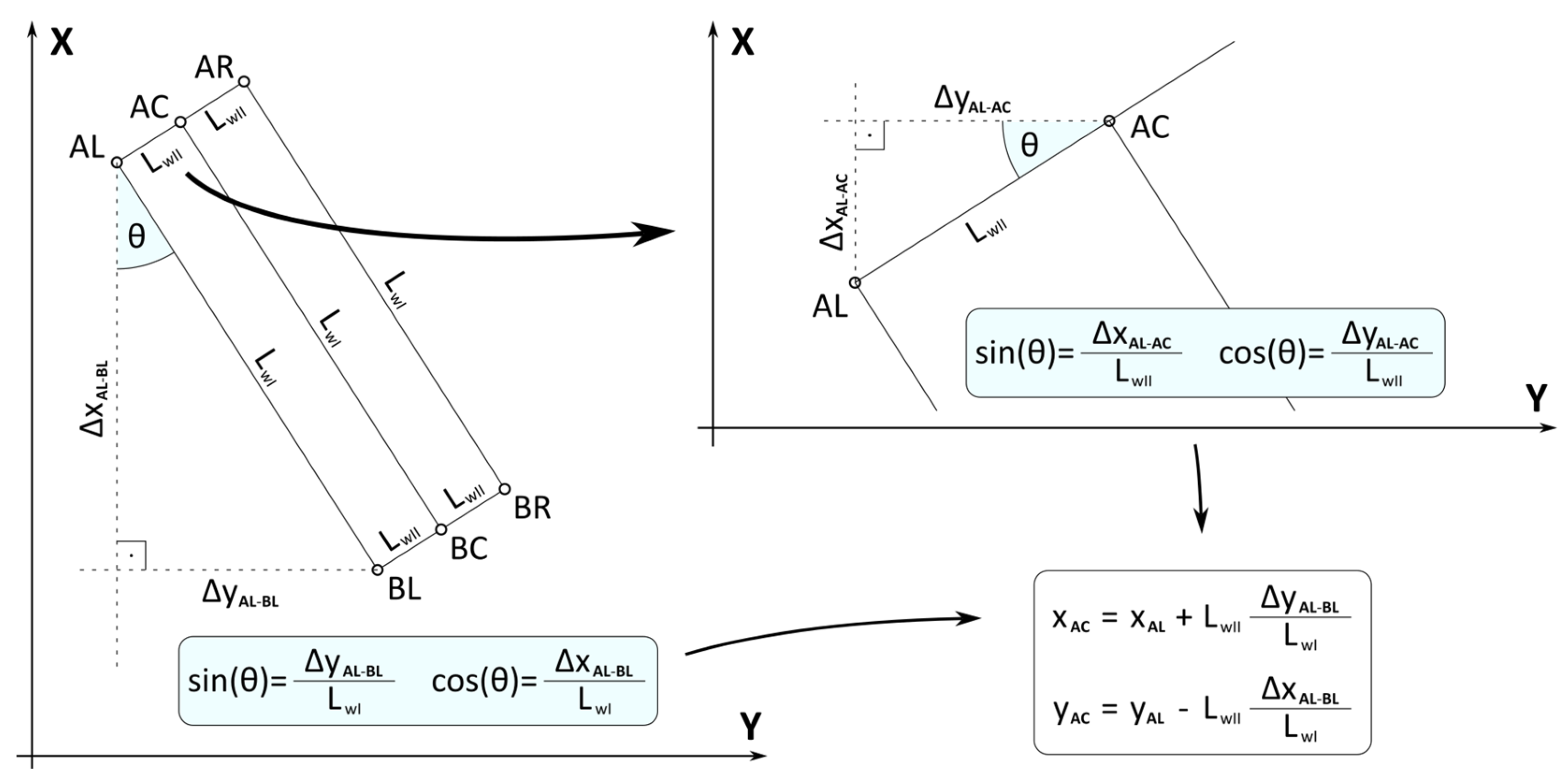
2.4. Algorithm for Determining the Correction of Track Axis Coordinates

The proposed algorithm is fully analytical, relying on explicit equations to compute corrected track axis coordinates. In this measurement scheme, two primary receivers—mounted above the bogie pivot pins—nominally define the track axis. However, as noted earlier, each of the six antenna positions carries random uncertainty due to varying measurement quality factors. Consequently, the track axis coordinates are derived using all six GNSS observations to mitigate individual receiver errors.

The core of the algorithm is the definition of logical conditions that determine whether the computed inter-antenna distances at each epoch satisfy predefined quality thresholds. These conditions are evaluated independently for each set of instantaneous antenna positions, with threshold values chosen by the analyst. Given that modern GNSS techniques—using RTK/RTN corrections or precise SP3 orbit post-processing—can achieve centimeter-level accuracy, this study adopts a quality tolerance of 1 to 5 cm.

In general, the quality conditions defined subsequently involve logical comparisons between the instantaneous antenna configurations and a reference model of control distances (L₁ through L₁₅).

2.4.1. Definition of Quality Conditions

In this method, the distance vectors between GNSS antennas—referred to as control distances—are central. Each antenna pair maintains a predefined reference distance. At each epoch, the absolute difference between the measured and reference distance for a given pair is compared against a quality threshold, ΔL_max. If the difference does not exceed ΔL_max, the pair is deemed to be within tolerance.

The fundamental quality check for a GNSS receiver’s measurement is satisfied if at least one of the following conditions holds:

• At least two control distances between the considered receiver and the others must fall within the assumed tolerance, including

  ○

  At least one “short” distance.

  ○

  At least one “long” distance.

• All “long” control distances from the considered receiver must be within the accepted tolerance.

For example, for the AC receiver, the measurement result (horizontal coordinates X, Y) meets the quality requirements only when the following logical condition is evaluated as TRUE:

$$W_{\mathrm{A}\mathrm{C}}:{\displaystyle \left[\begin{array}{c}\left[\left(\left|L_2-L_{\mathrm{w}\mathrm{I}}\right|\le ∆L_{\mathrm{m}\mathrm{a}\mathrm{x}}\right)\wedge \left(\left|L_6-L_{\mathrm{w}\mathrm{I}\mathrm{I}}\right|\le ∆L_{\mathrm{m}\mathrm{a}\mathrm{x}}\right)\right]\vee \left[\left(\left|L_2-L_{\mathrm{w}\mathrm{I}}\right|\le ∆L_{\mathrm{m}\mathrm{a}\mathrm{x}}\right)\wedge \left(\left|L_7-L_{\mathrm{w}\mathrm{I}\mathrm{I}}\right|\le ∆L_{\mathrm{m}\mathrm{a}\mathrm{x}}\right)\right]\vee \\ \vee \left[\left(\left|L_{12}-L_{\mathrm{w}\mathrm{V}}\right|\le ∆L_{\mathrm{m}\mathrm{a}\mathrm{x}}\right)\wedge \left(\left|L_6-L_{\mathrm{w}\mathrm{I}\mathrm{I}}\right|\le ∆L_{\mathrm{m}\mathrm{a}\mathrm{x}}\right)\right]\vee \left[\left(\left|L_{12}-L_{\mathrm{w}\mathrm{V}}\right|\le ∆L_{\mathrm{m}\mathrm{a}\mathrm{x}}\right)\wedge \left(\left|L_7-L_{\mathrm{w}\mathrm{I}\mathrm{I}}\right|\le ∆L_{\mathrm{m}\mathrm{a}\mathrm{x}}\right)\right]\vee \\ \vee \left[\left(\left|L_{14}-L_{\mathrm{w}\mathrm{V}}\right|\le ∆L_{\mathrm{m}\mathrm{a}\mathrm{x}}\right)\wedge \left(\left|L_6-L_{\mathrm{w}\mathrm{I}\mathrm{I}}\right|\le ∆L_{\mathrm{m}\mathrm{a}\mathrm{x}}\right)\right]\vee \left[\left(\left|L_{14}-L_{\mathrm{w}\mathrm{V}}\right|\le ∆L_{\mathrm{m}\mathrm{a}\mathrm{x}}\right)\wedge \left(\left|L_7-L_{\mathrm{w}\mathrm{I}\mathrm{I}}\right|\le ∆L_{\mathrm{m}\mathrm{a}\mathrm{x}}\right)\right]\vee \\ \vee \left[\left(\left|L_{12}-L_{\mathrm{w}\mathrm{V}}\right|\le ∆L_{\mathrm{m}\mathrm{a}\mathrm{x}}\right)\wedge \left(\left|L_2-L_{\mathrm{w}\mathrm{I}}\right|\le ∆L_{\mathrm{m}\mathrm{a}\mathrm{x}}\right)\wedge \left(\left|L_{14}-L_{\mathrm{w}\mathrm{V}}\right|\le ∆L_{\mathrm{m}\mathrm{a}\mathrm{x}}\right)\right]\end{array}\right]}$$

(10)

Logical conditions were similarly established for the other receivers. Consequently, by identifying which GNSS receivers yield measurements that meet the quality criteria at each epoch—and by applying the corresponding relationships—it is possible to compute the track axis coordinates even when some receivers do not provide sufficiently accurate data at that time.

2.4.2. Calculation of the Corrected Coordinate Values

Upon evaluating each receiver based on condition (10), it becomes possible to identify those that satisfy the predefined quality criteria. The coordinates of receivers condition (10) evaluates as TRUE form the input dataset for the algorithm responsible for computing the corrected positions of the central receivers AC and BC. Receivers for which the condition evaluates to FALSE are excluded from further analysis. The coordinates of the main receivers’ antennas, AC and BC—positioned directly above the pivots of the platform’s rotational axis—provide a precise and sufficient representation of the track axis location.

The logical structure associated with the availability of individual receivers (i.e., those satisfying condition (10)) allows for the definition of nine possible configurations for computing the corrected coordinates of receiver AC, and likewise, nine configurations for receiver BC. The first three configurations pertain to scenarios in which either receiver AC or more than one receiver from group A is available. In these cases, the corrected coordinates are derived exclusively from the available receivers within group A. The remaining configurations (4 through 9) address situations in which only a single receiver from group A is available (i.e., either AL or AR). In such instances, the computation of the resulting position of the AC receiver’s antenna necessitates the inclusion of at least one receiver from group B to determine the spatial orientation of the receiver layout, and consequently, the spatial orientation of the measurement platform itself.

Below are the equations describing the variants for the pivot receiver AC. The relationships for receiver BC are analogous.

Variant 1—All receivers within group A are available, whereas the availability of receivers within group B is optional.

$$W_1:\left[\begin{array}{c}\left[W_{AC}\wedge W_{AL}\wedge W_{AR}\wedge \left(W_{BC}\vee W_{BL}\vee W_{BR}\right)\right]\vee \\ \vee \left[W_{AC}\wedge W_{AL}\wedge W_{AR}\wedge \neg W_{BC}\wedge {\neg W}_{BL}\wedge \neg W_{BR}\right]\end{array}\right]$$

(11)

Corrected AC receiver coordinates:

$$Y_{\mathrm{A}\mathrm{C}1\prime }={\displaystyle \frac{Y_{\mathrm{A}\mathrm{C}}+Y_{\mathrm{A}\mathrm{L}}+Y_{\mathrm{A}\mathrm{R}}}{3}}$$

(12)

$$X_{\mathrm{A}\mathrm{C}1\prime }={\displaystyle \frac{X_{\mathrm{A}\mathrm{C}}+X_{\mathrm{A}\mathrm{L}}+X_{\mathrm{A}\mathrm{R}}}{3}}$$

(13)

Variant 2—Receivers AL and AR are available, while receiver AC is unavailable, and receivers from group B may or may not be available.

Logical condition:

$$W_2:\left[\begin{array}{c}\left[\neg W_{AC}\wedge W_{AL}\wedge W_{AR}\wedge \left(W_{BC}\vee W_{BL}\vee W_{BR}\right)\right]\vee \\ \vee \left[\neg W_{AC}\wedge W_{AL}\wedge W_{AR}\wedge \neg W_{BC}\wedge {\neg W}_{BL}\wedge \neg W_{BR}\right]\end{array}\right]$$

(14)

Corrected receiver coordinates:

$$Y_{\mathrm{A}\mathrm{C}2\prime }={\displaystyle \frac{Y_{\mathrm{A}\mathrm{L}}+Y_{\mathrm{A}\mathrm{R}}}{2}}$$

(15)

$$X_{\mathrm{A}\mathrm{C}2\prime }={\displaystyle \frac{X_{\mathrm{A}\mathrm{L}}+X_{\mathrm{A}\mathrm{R}}}{2}}$$

(16)

Variant 3—Receivers AC and AL, or AC and AR, are available, while receivers from group B may or may not be available.

Logical condition:

$$W_3:\left[\begin{array}{c}\left[W_{\mathrm{A}\mathrm{C}}\wedge \neg W_{\mathrm{A}\mathrm{L}}\wedge W_{\mathrm{A}\mathrm{R}}\wedge \left(W_{\mathrm{B}\mathrm{C}}\vee W_{\mathrm{B}\mathrm{L}}\vee W_{\mathrm{B}\mathrm{R}}\right)\right]\vee \left[W_{\mathrm{A}\mathrm{C}}\wedge W_{\mathrm{A}\mathrm{L}}\wedge \neg W_{\mathrm{A}\mathrm{R}}\wedge \left(W_{\mathrm{B}\mathrm{C}}\vee W_{\mathrm{B}\mathrm{L}}\vee W_{\mathrm{B}\mathrm{R}}\right)\right]\vee \\ \vee \left[W_{\mathrm{A}\mathrm{C}}\wedge \neg W_{\mathrm{A}\mathrm{L}}\wedge \neg W_{\mathrm{A}\mathrm{R}}\wedge \left(W_{\mathrm{B}\mathrm{C}}\vee W_{\mathrm{B}\mathrm{L}}\vee W_{\mathrm{B}\mathrm{R}}\right)\right]\vee \left[W_{\mathrm{A}\mathrm{C}}\wedge W_{\mathrm{A}\mathrm{L}}\wedge \neg W_{\mathrm{A}\mathrm{R}}\wedge \neg W_{\mathrm{B}\mathrm{C}}\wedge {\neg W}_{\mathrm{B}\mathrm{L}}\wedge \neg W_{\mathrm{B}\mathrm{R}}\right]\vee \\ \vee \left[W_{\mathrm{A}\mathrm{C}}\wedge {\neg W}_{\mathrm{A}\mathrm{L}}\wedge W_{\mathrm{A}\mathrm{R}}\wedge \neg W_{\mathrm{B}\mathrm{C}}\wedge {\neg W}_{\mathrm{B}\mathrm{L}}\wedge \neg W_{\mathrm{B}\mathrm{R}}\right]\end{array}\right]$$

(17)

Corrected receiver coordinates:

$$Y_{\mathrm{A}\mathrm{C}3\prime }=Y_{\mathrm{A}\mathrm{C}}$$

(18)

$$X_{\mathrm{A}\mathrm{C}3\prime }=X_{\mathrm{A}\mathrm{C}}$$

(19)

Variant 4—Within group A, only receiver AL is available, whereas within group B, receiver BL is available.

Logical condition:

$$W_4:\left[\neg W_{\mathrm{A}\mathrm{C}}\wedge W_{\mathrm{A}\mathrm{L}}\wedge \neg W_{\mathrm{A}\mathrm{R}}\wedge W_{\mathrm{B}\mathrm{L}}\right]$$

(20)

Corrected receiver coordinates are determined based on the vertices and the horizontal azimuth angle of the transversal segment, as well as the theoretical distances between the receivers (2)–(4):

$$Y_{\mathrm{A}\mathrm{C}4\prime }=Y_{\mathrm{A}\mathrm{L}}+L_{\mathrm{w}\mathrm{I}\mathrm{I}}\cdot \left({\displaystyle \frac{X_{\mathrm{A}\mathrm{L}}-X_{\mathrm{B}\mathrm{L}}}{L_{\mathrm{w}\mathrm{I}}}}\right)$$

(21)

$$X_{\mathrm{A}\mathrm{C}4\prime }=X_{\mathrm{A}\mathrm{L}}-L_{\mathrm{w}\mathrm{I}\mathrm{I}}\cdot \left({\displaystyle \frac{Y_{\mathrm{A}\mathrm{L}}-Y_{\mathrm{B}\mathrm{L}}}{L_{\mathrm{w}\mathrm{I}}}}\right)$$

(22)

For improved clarity of the equations describing the coordinates of receiver AC, the geometric relationships are illustrated below in Figure 4.

Variant 5—Within group A, only receiver AL is available, while within group B, receiver BC is available in the absence of receiver BL.

Logical condition:

$$W_5:\left[\neg W_{\mathrm{A}\mathrm{C}}\wedge W_{\mathrm{A}\mathrm{L}}\wedge \neg W_{\mathrm{A}\mathrm{R}}\wedge \neg W_{\mathrm{B}\mathrm{L}}\wedge W_{\mathrm{B}\mathrm{C}}\right]$$

(23)

Corrected receiver coordinates, in addition to using the transversal line path as shown in variant 4, are determined by taking into account the oblique course of the segment between the central and lateral receiver (cf. Figure 3b):

$$Y_{\mathrm{A}\mathrm{C}5\prime }=Y_{\mathrm{A}\mathrm{L}}+\left[L_{\mathrm{w}\mathrm{I}\mathrm{I}}\cdot \left({\displaystyle \frac{X_{\mathrm{A}\mathrm{L}}-X_{\mathrm{B}\mathrm{C}}}{L_{\mathrm{w}\mathrm{V}}}}\right)\cdot \cos \left[-{\tan }^{-1}\left({\displaystyle \frac{L_{\mathrm{w}\mathrm{I}\mathrm{I}}}{L_{\mathrm{w}\mathrm{I}}}}\right)\right]-\left(-L_{\mathrm{w}\mathrm{I}\mathrm{I}}\cdot \left({\displaystyle \frac{Y_{\mathrm{A}\mathrm{L}}-Y_{\mathrm{B}\mathrm{C}}}{L_{\mathrm{w}\mathrm{V}}}}\right)\right)\cdot \sin \left[-{\tan }^{-1}\left({\displaystyle \frac{L_{\mathrm{w}\mathrm{I}\mathrm{I}}}{L_{\mathrm{w}\mathrm{I}}}}\right)\right]\right]$$

(24)

$$X_{\mathrm{A}\mathrm{C}5\prime }=X_{\mathrm{A}\mathrm{L}}+\left[L_{\mathrm{w}\mathrm{I}\mathrm{I}}\cdot \left({\displaystyle \frac{X_{\mathrm{A}\mathrm{L}}-X_{\mathrm{B}\mathrm{C}}}{L_{\mathrm{w}\mathrm{V}}}}\right)\cdot \sin \left[-{\tan }^{-1}\left({\displaystyle \frac{L_{\mathrm{wII}}}{L_{\mathrm{wI}}}}\right)\right]+\left(-L_{\mathrm{w}\mathrm{I}\mathrm{I}}\cdot \left({\displaystyle \frac{Y_{\mathrm{A}\mathrm{L}}-Y_{\mathrm{B}\mathrm{C}}}{L_{\mathrm{w}\mathrm{V}}}}\right)\right)\cdot \cos \left[-{\tan }^{-1}\left({\displaystyle \frac{L_{\mathrm{w}\mathrm{I}\mathrm{I}}}{L_{\mathrm{w}\mathrm{I}}}}\right)\right]\right]$$

(25)

Variant 6—Within group A, only receiver AL is available, while within group B, receiver BR is available in the absence of receivers BL and BC.

Logical condition:

$$W_6:\left[\neg W_{\mathrm{A}\mathrm{C}}\wedge W_{\mathrm{A}\mathrm{L}}\wedge \neg W_{\mathrm{A}\mathrm{R}}\wedge \neg W_{\mathrm{B}\mathrm{L}}\wedge {\neg W}_{\mathrm{B}\mathrm{C}}\wedge W_{\mathrm{B}\mathrm{R}}\right]$$

(26)

Corrected receiver coordinates are determined by taking into account the diagonal course between the alternately positioned receivers (cf. Figure 3b):

$$Y_{\mathrm{A}\mathrm{C}6\prime }=Y_{\mathrm{A}\mathrm{L}}+\left[L_{\mathrm{w}\mathrm{I}\mathrm{I}}\cdot \left({\displaystyle \frac{X_{\mathrm{A}\mathrm{L}}-X_{\mathrm{B}\mathrm{R}}}{L_{\mathrm{w}\mathrm{I}\mathrm{V}}}}\right)\cdot \cos \left[-{\tan }^{-1}\left({\displaystyle \frac{L_{\mathrm{w}\mathrm{I}\mathrm{I}\mathrm{I}}}{L_{\mathrm{w}\mathrm{I}}}}\right)\right]-\left(-L_{\mathrm{w}\mathrm{I}\mathrm{I}}\cdot \left({\displaystyle \frac{Y_{\mathrm{A}\mathrm{L}}-Y_{\mathrm{B}\mathrm{R}}}{L_{\mathrm{w}\mathrm{I}\mathrm{V}}}}\right)\right)\cdot \sin \left[-{\tan }^{-1}\left({\displaystyle \frac{L_{\mathrm{w}\mathrm{I}\mathrm{I}\mathrm{I}}}{L_{\mathrm{w}\mathrm{I}}}}\right)\right]\right]$$

(27)

$$X_{\mathrm{A}\mathrm{C}6\prime }=X_{\mathrm{A}\mathrm{L}}+\left[L_{\mathrm{w}\mathrm{I}\mathrm{I}}\cdot \left({\displaystyle \frac{X_{\mathrm{A}\mathrm{L}}-X_{\mathrm{B}\mathrm{R}}}{L_{\mathrm{w}\mathrm{I}\mathrm{V}}}}\right)\cdot \sin \left[-{\tan }^{-1}\left({\displaystyle \frac{L_{\mathrm{wIII}}}{L_{\mathrm{wI}}}}\right)\right]+\left(-L_{\mathrm{w}\mathrm{I}\mathrm{I}}\cdot \left({\displaystyle \frac{Y_{\mathrm{A}\mathrm{L}}-Y_{\mathrm{B}\mathrm{R}}}{L_{\mathrm{w}\mathrm{I}\mathrm{V}}}}\right)\right)\cdot \cos \left[-{\tan }^{-1}\left({\displaystyle \frac{L_{\mathrm{w}\mathrm{I}\mathrm{I}\mathrm{I}}}{L_{\mathrm{w}\mathrm{I}}}}\right)\right]\right]$$

(28)

Variant 7—within group A, only receiver AR is available, whereas within group B, receiver BR is available.

Logical condition:

$$W_7:\left[\neg W_{\mathrm{A}\mathrm{C}}\wedge \neg W_{\mathrm{A}\mathrm{L}}\wedge W_{\mathrm{A}\mathrm{R}}\wedge W_{\mathrm{B}\mathrm{R}}\right]$$

(29)

Corrected receiver coordinates are determined similarly to variant 4, with the difference that the two utilized receivers form the right longitudinal segment:

$$Y_{\mathrm{A}\mathrm{C}7\prime }=Y_{\mathrm{A}\mathrm{R}}-L_{\mathrm{w}\mathrm{I}\mathrm{I}}\cdot \left({\displaystyle \frac{X_{\mathrm{A}\mathrm{R}}-X_{\mathrm{B}\mathrm{R}}}{L_{\mathrm{w}\mathrm{I}}}}\right)$$

(30)

$$X_{\mathrm{A}\mathrm{C}7\prime }=X_{\mathrm{A}\mathrm{R}}+L_{\mathrm{w}\mathrm{I}\mathrm{I}}\cdot \left({\displaystyle \frac{Y_{\mathrm{A}\mathrm{R}}-Y_{\mathrm{B}\mathrm{R}}}{L_{\mathrm{w}\mathrm{I}}}}\right)$$

(31)

Variant 8—within group A, only receiver AR is available, while within group B, receiver BC is available in the absence of receiver BR.

Logical condition:

$$W_8:\left[\neg W_{\mathrm{A}\mathrm{C}}\wedge \neg W_{\mathrm{A}\mathrm{L}}\wedge W_{\mathrm{A}\mathrm{R}}\wedge W_{\mathrm{B}\mathrm{C}}\wedge \neg W_{\mathrm{B}\mathrm{R}}\right]$$

(32)

Corrected receiver coordinates are determined symmetrically with respect to the configuration analogous to variant 5:

$$Y_{\mathrm{A}\mathrm{C}8\prime }=Y_{\mathrm{A}\mathrm{R}}+\left[-L_{\mathrm{w}\mathrm{I}\mathrm{I}}\cdot \left({\displaystyle \frac{X_{\mathrm{A}\mathrm{R}}-X_{\mathrm{B}\mathrm{C}}}{L_{\mathrm{w}\mathrm{V}}}}\right)\cdot \cos \left[{\tan }^{-1}\left({\displaystyle \frac{L_{\mathrm{w}\mathrm{I}\mathrm{I}}}{L_{\mathrm{w}\mathrm{I}}}}\right)\right]-\left(L_{\mathrm{w}\mathrm{I}\mathrm{I}}\cdot \left({\displaystyle \frac{Y_{\mathrm{A}\mathrm{R}}-Y_{\mathrm{B}\mathrm{C}}}{L_{\mathrm{w}\mathrm{V}}}}\right)\right)\cdot \sin \left[{\tan }^{-1}\left({\displaystyle \frac{L_{\mathrm{w}\mathrm{I}\mathrm{I}}}{L_{\mathrm{w}\mathrm{I}}}}\right)\right]\right]$$

(33)

$$X_{\mathrm{A}\mathrm{C}8\prime }=X_{\mathrm{A}\mathrm{R}}+\left[-L_{\mathrm{w}\mathrm{I}\mathrm{I}}\cdot \left({\displaystyle \frac{X_{\mathrm{A}\mathrm{R}}-X_{\mathrm{B}\mathrm{C}}}{L_{\mathrm{w}\mathrm{V}}}}\right)\cdot \sin \left[{\tan }^{-1}\left({\displaystyle \frac{L_{\mathrm{wII}}}{L_{\mathrm{wI}}}}\right)\right]+\left(L_{\mathrm{w}\mathrm{I}\mathrm{I}}\cdot \left({\displaystyle \frac{Y_{\mathrm{A}\mathrm{R}}-Y_{\mathrm{B}\mathrm{C}}}{L_{\mathrm{w}\mathrm{V}}}}\right)\right)\cdot \cos \left[{\tan }^{-1}\left({\displaystyle \frac{L_{\mathrm{w}\mathrm{I}\mathrm{I}}}{L_{\mathrm{w}\mathrm{I}}}}\right)\right]\right]$$

(34)

Variant 9—within group A, only receiver AR is available, while within group B, receiver BL is available in the absence of receivers BR and BC.

Logical condition:

$$W_9:\left[\neg W_{\mathrm{A}\mathrm{C}}\wedge {\neg W}_{\mathrm{A}\mathrm{L}}\wedge W_{\mathrm{A}\mathrm{R}}\wedge {\neg W}_{\mathrm{B}\mathrm{C}}\wedge W_{\mathrm{B}\mathrm{L}}\wedge \neg W_{\mathrm{B}\mathrm{R}}\right]$$

(35)

Corrected receiver coordinates are determined symmetrically with respect to diagonal variant 6:

$$Y_{\mathrm{A}\mathrm{C}9\prime }=Y_{\mathrm{A}\mathrm{R}}+\left[-L_{\mathrm{w}\mathrm{I}\mathrm{I}}\cdot \left({\displaystyle \frac{X_{\mathrm{A}\mathrm{R}}-X_{\mathrm{B}\mathrm{L}}}{L_{\mathrm{w}\mathrm{I}\mathrm{V}}}}\right)\cdot \cos \left[{\tan }^{-1}\left({\displaystyle \frac{L_{\mathrm{w}\mathrm{I}\mathrm{I}\mathrm{I}}}{L_{\mathrm{w}\mathrm{I}}}}\right)\right]-\left(L_{\mathrm{w}\mathrm{I}\mathrm{I}}\cdot \left({\displaystyle \frac{Y_{\mathrm{A}\mathrm{R}}-Y_{\mathrm{B}\mathrm{L}}}{L_{\mathrm{w}\mathrm{I}\mathrm{V}}}}\right)\right)\cdot \sin \left[{\tan }^{-1}\left({\displaystyle \frac{L_{\mathrm{w}\mathrm{I}\mathrm{I}\mathrm{I}}}{L_{\mathrm{w}\mathrm{I}}}}\right)\right]\right]$$

(36)

$$X_{\mathrm{A}\mathrm{C}9\prime }=X_{\mathrm{A}\mathrm{R}}+\left[-L_{\mathrm{w}\mathrm{I}\mathrm{I}}\cdot \left({\displaystyle \frac{X_{\mathrm{A}\mathrm{R}}-X_{\mathrm{B}\mathrm{L}}}{L_{\mathrm{w}\mathrm{I}\mathrm{V}}}}\right)\cdot \sin \left[{\tan }^{-1}\left({\displaystyle \frac{L_{\mathrm{wIII}}}{L_{\mathrm{wI}}}}\right)\right]+\left(L_{\mathrm{w}\mathrm{I}\mathrm{I}}\cdot \left({\displaystyle \frac{Y_{\mathrm{A}\mathrm{R}}-Y_{\mathrm{B}\mathrm{L}}}{L_{\mathrm{w}\mathrm{I}\mathrm{V}}}}\right)\right)\cdot \cos \left[{\tan }^{-1}\left({\displaystyle \frac{L_{\mathrm{w}\mathrm{I}\mathrm{I}\mathrm{I}}}{L_{\mathrm{w}\mathrm{I}}}}\right)\right]\right]$$

(37)

In the situation where none of the above variants are met, we are dealing with the so-called negative variant, which means that it is not possible to obtain a measurement result that meets the requirements for an acceptable level of uncertainty. In such a case, the measurement sample from the given measurement epoch should be omitted.

Considering only the positive variants that meet the criteria for an acceptable level of uncertainty, the resultant measurement result for receiver AC will be described by the following relation:

$$Y_{\mathrm{A}\mathrm{C}\prime }={\sum }_{i=1}^9{W}_i\cdot Y_{\mathrm{A}\mathrm{C}i\prime }$$

(38)

$$X_{\mathrm{A}\mathrm{C}\prime }={\sum }_{i=1}^9{W}_i\cdot X_{\mathrm{A}\mathrm{C}i\prime }$$

(39)

The relationships for receiver BC will be analogous.

Since no control algorithm is perfect, there may be cases in which a measurement affected by significant uncertainty is mistakenly accepted as correct. For this reason, an additional control criterion was introduced, which involves checking the length of the so-called fixed base—that is, the distance between receivers AC and BC after correction using the control algorithm.

The length of the fixed base ($L_{\mathrm{F}\mathrm{B}}$) for the corrected coordinates of AC and BC is given by the following relation:

$$L_{\mathrm{F}\mathrm{B}\_\mathrm{c}\mathrm{o}\mathrm{r}\mathrm{r}}=\sqrt{{\left(X_{\mathrm{A}\mathrm{C}\prime }-X_{\mathrm{B}\mathrm{C}\prime }\right)}^2+{\left(Y_{\mathrm{A}\mathrm{C}\prime }-Y_{\mathrm{B}\mathrm{C}\prime }\right)}^2}$$

(40)

while the additional condition checking the quality of the measurement result in terms of calibration uncertainty is given by

$$u_{\mathrm{F}\mathrm{B}}:\left[\left|L_{\mathrm{F}\mathrm{B}\_\mathrm{c}\mathrm{o}\mathrm{r}\mathrm{r}}-L_{\mathrm{w}\mathrm{I}}\right|\le \Delta L_{\mathrm{F}\mathrm{B}}\right]$$

(41)

where

• $u_{\mathrm{F}\mathrm{B}}$ refers to the calibration uncertainty of fixed base [m].
• $L_{\mathrm{F}\mathrm{B}\_\mathrm{c}\mathrm{o}\mathrm{r}\mathrm{r}}$ is the fixed base length derived from the corrected coordinates of antennas AC- BC.
• $L_{\mathrm{w}\mathrm{I}}$ is the reference distance (compare Figure 2 with Equations (2) and (5)).
• $\Delta L_{\mathrm{F}\mathrm{B}}$ is the assumed acceptable fixed base uncertainty (arbitrary value).

3. Results

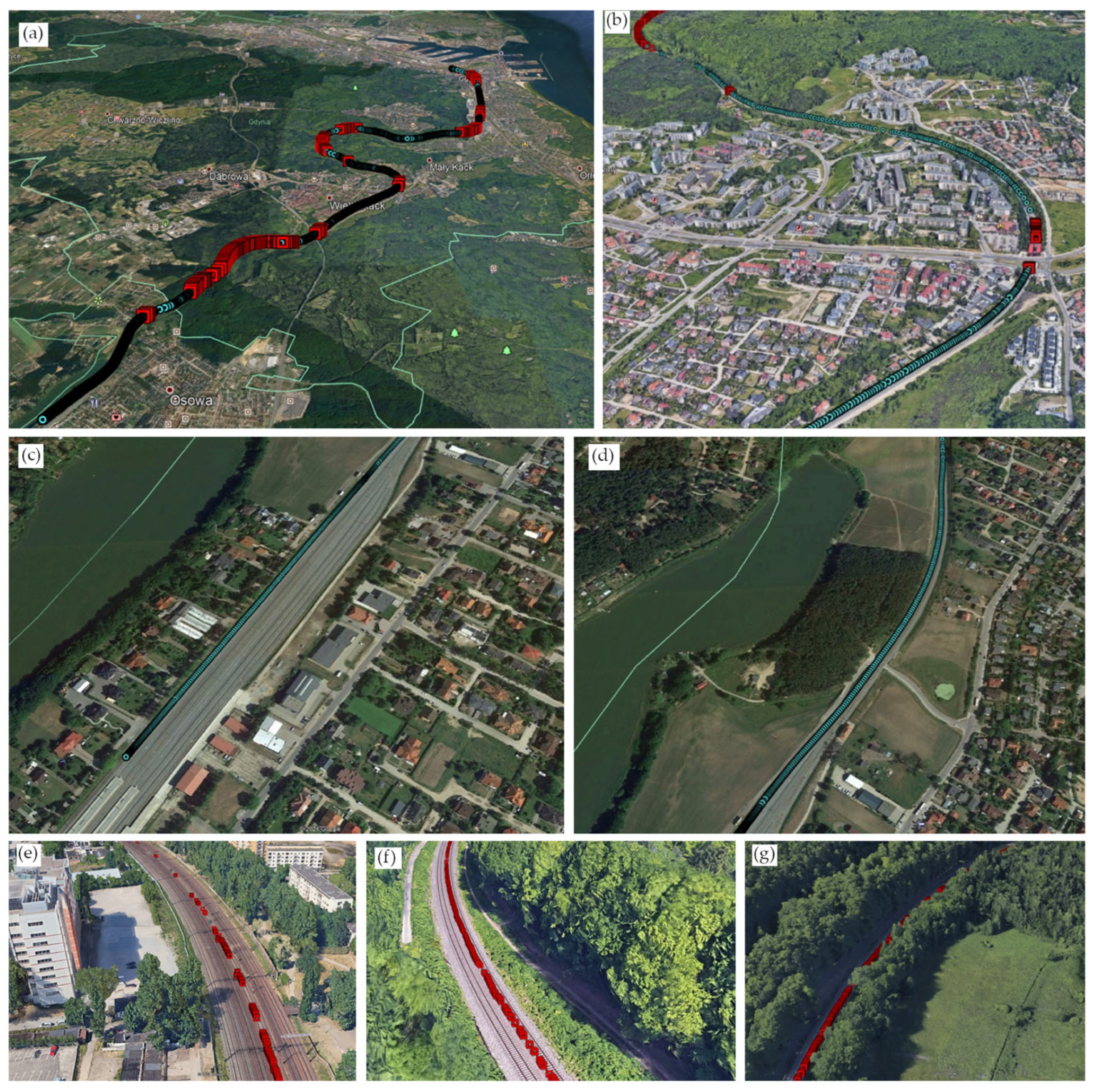
3.1. Results of Measurements—Evaluation of Algorithm Effectiveness

To validate the theoretical framework, the described algorithm was implemented to evaluate the track axis computed from mobile GNSS measurements on an operational railway line. The measurement platform carried six geodetic GNSS receivers arranged as shown in Figure 3b. During data acquisition, real-time RTK (Real-Time Kinematic) corrections were applied, and IMU measurements recorded platform tilt angles. Figure 5a illustrates the measured railway route in red, while Figure 5b depicts the computed track axis for the Osowa–Gdynia segment. Blue points denote high-quality positions—where the fixed-base deviation was under 1 cm—and red points denote low-quality positions, with deviations up to 20 cm. The fixed-base length for each epoch was computed according to Equation (42).

$$L_{\mathrm{F}\mathrm{B}}=\sqrt{{\left(X_{\mathrm{A}\mathrm{C}}-X_{\mathrm{B}\mathrm{C}}\right)}^2+{\left(Y_{\mathrm{A}\mathrm{C}}-Y_{\mathrm{B}\mathrm{C}}\right)}^2}$$

(42)

The selected route features complex geometry in both plan and longitudinal profiles, with numerous terrain obstructions that impede satellite signal reception. The urban segment from Gdańsk Główny to Gdańsk Wrzeszcz traverses a densely built environment, punctuated by viaducts and other infrastructural barriers. In contrast, the stretch from Gdańsk Wrzeszcz through Gdańsk Osowa to Gdynia Główna resembles a mountainous line, with tight curves and steep longitudinal gradients. Much of this section runs through forested areas and deep cuttings, and is intersected by footbridges, bridges, and similar obstacles. These conditions reduce satellite visibility and challenge GNSS-based measurements, making the route an ideal testbed for validating the proposed method’s robustness.

Figure 6 presents the measurement results in the form of coordinate points of the track axis overlaid on an orthophotomap. The points are divided on a similar basis: blue points represent high quality (${\Delta L}_{\mathrm{F}\mathrm{B}}<1 \mathrm{c}\mathrm{m}$), while red points indicate low-accuracy measurements (${\Delta L}_{\mathrm{F}\mathrm{B}}>20 \mathrm{c}\mathrm{m}$). Figure 6a shows the measurement of the entire section from Osowa to Gdynia. Figure 6b illustrates the route in an open area, where the quality is only reduced at one location due to a viaduct acting as an infrastructural obstruction. Figure 6c,d present sections of the line located in open terrain without point obstructions. Figure 6e demonstrates the impact of high-rise buildings characteristic of urbanized areas, whereas Figure 6f,g indicate the influence of obstructions in the form of trees located close to the track.

From an uncertainty-analysis standpoint, it is notable that both high- and low-quality measurements tend to cluster into relatively long route segments, with only isolated obstructions (e.g., viaducts, tall buildings) breaking these clusters. This creates an undesirable outcome for track inventory: entire horizontal curves—or even sequences of curves—may be excluded due to prolonged sections of insufficient accuracy. Such extended low-quality segments also hinder precise reconstruction of the track’s horizontal geometric layout.

3.2. Effectiveness of the Algorithm

The effectiveness of the proposed algorithm was demonstrated by comparing the expanded uncertainty associated with determining the AB vector, $L_{FB}$, between the base antennas positioned above the bogie pivot points. The fixed-base LFBLFB was computed at each position along the identified track axis. In the typical approach—using the planar coordinates of the antennas along with their standard uncertainties (CQ2D)—the expanded uncertainty, $U_{FB}^{CQ2D}$, was calculated using the metrological method recommended in [32]. This method is defined by the following equations:

$$L_{\mathrm{F}\mathrm{B}}=\sqrt{{\left(X_{\mathrm{A}\mathrm{C}}-X_{\mathrm{B}\mathrm{C}}\right)}^2+{\left(Y_{\mathrm{A}\mathrm{C}}-Y_{\mathrm{B}\mathrm{C}}\right)}^2}$$

(43)

$${\displaystyle \frac{\partial L_{\mathrm{F}\mathrm{B}}}{\partial X_{\mathrm{A}\mathrm{C}}}}={\displaystyle \frac{X_{\mathrm{A}\mathrm{C}}-X_{\mathrm{B}\mathrm{C}}}{\sqrt{{\left(X_{\mathrm{A}\mathrm{C}}-X_{\mathrm{B}\mathrm{C}}\right)}^2+{\left(Y_{\mathrm{A}\mathrm{C}}-Y_{\mathrm{B}\mathrm{C}}\right)}^2}}}$$

(44)

$${\displaystyle \frac{\partial L_{\mathrm{F}\mathrm{B}}}{\partial X_{\mathrm{B}\mathrm{C}}}}={\displaystyle \frac{-X_{\mathrm{A}\mathrm{C}}+X_{\mathrm{B}\mathrm{C}}}{\sqrt{{\left(X_{\mathrm{A}\mathrm{C}}-X_{\mathrm{B}\mathrm{C}}\right)}^2+{\left(Y_{\mathrm{A}\mathrm{C}}-Y_{\mathrm{B}\mathrm{C}}\right)}^2}}}$$

(45)

$${\displaystyle \frac{\partial L_{\mathrm{F}\mathrm{B}}}{\partial Y_{\mathrm{A}\mathrm{C}}}}={\displaystyle \frac{Y_{\mathrm{A}\mathrm{C}}-Y_{\mathrm{B}\mathrm{C}}}{\sqrt{{\left(X_{\mathrm{A}\mathrm{C}}-X_{\mathrm{B}\mathrm{C}}\right)}^2+{\left(Y_{\mathrm{A}\mathrm{C}}-Y_{\mathrm{B}\mathrm{C}}\right)}^2}}}$$

(46)

$${\displaystyle \frac{\partial L_{\mathrm{F}\mathrm{B}}}{\partial Y_{\mathrm{B}\mathrm{C}}}}={\displaystyle \frac{-Y_{\mathrm{A}\mathrm{C}}+Y_{\mathrm{B}\mathrm{C}}}{\sqrt{{\left(X_{\mathrm{A}\mathrm{C}}-X_{\mathrm{B}\mathrm{C}}\right)}^2+{\left(Y_{\mathrm{A}\mathrm{C}}-Y_{\mathrm{B}\mathrm{C}}\right)}^2}}}$$

(47)

$$u_{FB}^{CQ2D}=\sqrt{{\left({\displaystyle \frac{\partial L_{\mathrm{F}\mathrm{B}}}{\partial X_{\mathrm{A}\mathrm{C}}}}\right)}^2·u^2\left(X_{\mathrm{A}\mathrm{C}}\right)+{\left({\displaystyle \frac{\partial L_{\mathrm{F}\mathrm{B}}}{\partial X_{\mathrm{B}\mathrm{C}}}}\right)}^2·u^2\left(X_{\mathrm{B}\mathrm{C}}\right)+{\left({\displaystyle \frac{\partial L_{\mathrm{F}\mathrm{B}}}{\partial Y_{\mathrm{A}\mathrm{C}}}}\right)}^2·u^2\left(Y_{\mathrm{A}\mathrm{C}}\right)+{\left({\displaystyle \frac{\partial L_{\mathrm{F}\mathrm{B}}}{\partial Y_{\mathrm{B}\mathrm{C}}}}\right)}^2·u^2\left(Y_{\mathrm{B}\mathrm{C}}\right)}$$

(48)

$$u_{FB}^{CQ2D}=\sqrt{\begin{array}{c}{\left({\displaystyle \frac{X_{\mathrm{A}\mathrm{C}}-X_{\mathrm{B}\mathrm{C}}}{\sqrt{{\left(X_{\mathrm{A}\mathrm{C}}-X_{\mathrm{B}\mathrm{C}}\right)}^2+{\left(Y_{\mathrm{A}\mathrm{C}}-Y_{\mathrm{B}\mathrm{C}}\right)}^2}}}\right)}^2·u^2\left(X_{\mathrm{A}\mathrm{C}}\right)+{\left({\displaystyle \frac{-X_{\mathrm{A}\mathrm{C}}+X_{\mathrm{B}\mathrm{C}}}{\sqrt{{\left(X_{\mathrm{A}\mathrm{C}}-X_{\mathrm{B}\mathrm{C}}\right)}^2+{\left(Y_{\mathrm{A}\mathrm{C}}-Y_{\mathrm{B}\mathrm{C}}\right)}^2}}}\right)}^2·u^2\left(X_{\mathrm{B}\mathrm{C}}\right)+\\ +{\left({\displaystyle \frac{Y_{\mathrm{A}\mathrm{C}}-Y_{\mathrm{B}\mathrm{C}}}{\sqrt{{\left(X_{\mathrm{A}\mathrm{C}}-X_{\mathrm{B}\mathrm{C}}\right)}^2+{\left(Y_{\mathrm{A}\mathrm{C}}-Y_{\mathrm{B}\mathrm{C}}\right)}^2}}}\right)}^2·u^2\left(Y_{\mathrm{A}\mathrm{C}}\right)+{\left({\displaystyle \frac{-Y_{\mathrm{A}\mathrm{C}}+Y_{\mathrm{B}\mathrm{C}}}{\sqrt{{\left(X_{\mathrm{A}\mathrm{C}}-X_{\mathrm{B}\mathrm{C}}\right)}^2+{\left(Y_{\mathrm{A}\mathrm{C}}-Y_{\mathrm{B}\mathrm{C}}\right)}^2}}}\right)}^2·u^2\left(Y_{\mathrm{B}\mathrm{C}}\right)\end{array}}$$

(49)

$$u\left(X_{\mathrm{A}\mathrm{C}}\right)=u\left(Y_{\mathrm{A}\mathrm{C}}\right)={\mathrm{C}\mathrm{Q}2\mathrm{D}}_{\mathrm{A}\mathrm{C}}$$

(50)

$$u\left(X_{\mathrm{B}\mathrm{C}}\right)=u\left(Y_{\mathrm{B}\mathrm{C}}\right)={\mathrm{C}\mathrm{Q}2\mathrm{D}}_{\mathrm{B}\mathrm{C}}$$

(51)

$$U_{FB}^{CQ2D}=k·u_{FB}^{CQ2D}=2·u_{FB}^{CQ2D}$$

(52)

$$U_{FB}={\displaystyle \frac{k}{\sqrt{3}}}·u_{FB}={\displaystyle \frac{2}{\sqrt{3}}}·u_{FB}$$

(53)

$$∆U={\displaystyle \frac{U_{FB}^{CQ2D}-U_{FB}}{U_{FB}^{CQ2D}}}·100\%$$

(54)

where

• $Y_{\mathrm{A}\mathrm{C}}, X_{\mathrm{A}\mathrm{C}}, Y_{\mathrm{B}\mathrm{C}}, X_{\mathrm{B}\mathrm{C}}$ are the base antennas coordinates in PL-2000 [m].
• $L_{\mathrm{F}\mathrm{B}}$ is the fixed base of a measurement wagon [m].
• $u_{FB}^{CQ2D}$ is the calculated standard uncertainty of fixed base [m].
• $u_{FB}$ is the calculated calibration uncertainty of fixed base [m].
• $U_{FB}^{CQ2D}$ is the calculated expanded uncertainty of fixed base [m].
• $U_{FB}$ is the calculated expanded uncertainty of fixed base [m].
• $k$ represents coverage factor k [-].
• $∆U$ represents the relative reduction in the expanded uncertainty of the fixed base [%].

The expanded uncertainty values of the fixed base, UFBUFB, calculated using the proposed algorithm, were evaluated using Formulas (41) and (53), assuming $\Delta L_{FB}=5 \mathrm{c}\mathrm{m}$. Using the above computational methodology, Figure 7, Figure 8, Figure 9, Figure 10 and Figure 11 present the compared expanded uncertainties, illustrating the effectiveness of the method along the analyzed track section. The horizontal axis of the plots represents time. For the purposes of computation, analysis, and clear presentation of the results, the entire route was divided into five sessions.

The analysis of the results presented in Figure 7, Figure 8, Figure 9, Figure 10 and Figure 11 allows us to draw conclusions regarding the effectiveness of the developed algorithm. In the majority of cases, i.e., where the algorithm successfully determines the fixed base length, the reduction in expanded uncertainty is clear, amounting to approximately an order of magnitude compared to the original values. In instances where determining $L_{\mathrm{F}\mathrm{B}}$ is not feasible due to insufficient reliable input data, the uncertainty comparisons are not meaningful. Including these instances in the plots (Figure 7, Figure 8, Figure 9, Figure 10 and Figure 11) highlights the number of track sections for which coordinates must be supplemented or replaced by data from alternative systems, such as INS. To further illustrate the algorithm’s performance, Figure 12 presents plots depicting the percentage reduction in expanded uncertainty alongside a histogram illustrating the distribution of these values—including sections that have been deemed unreliable due to low parameter values. The evaluation of these plots confirms the high efficacy of the proposed method. Numerical summaries of key statistics are provided in

Table 2. Basic statistics of the $∆U$ indicator for individual measurement sessions.

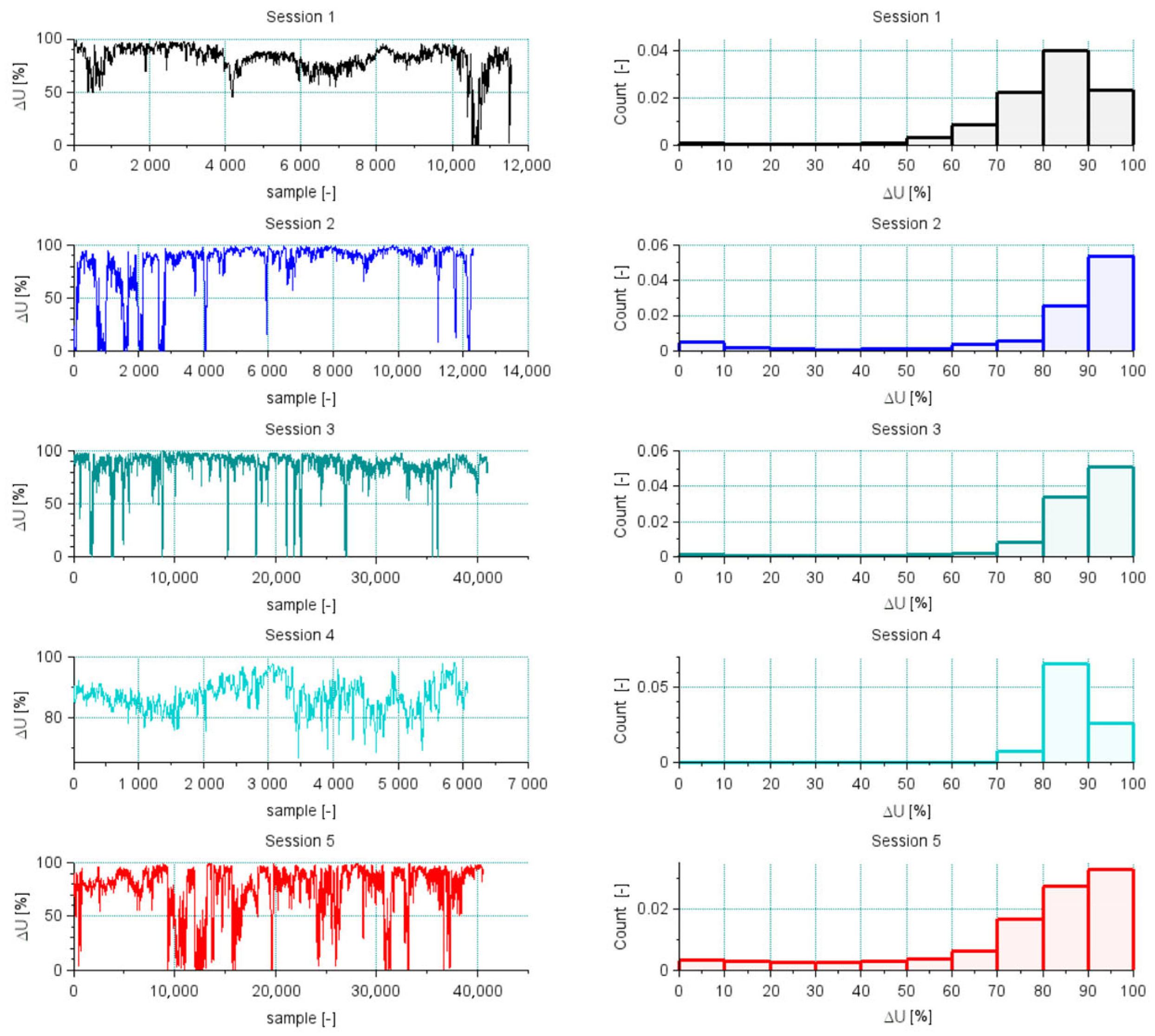
	Mean	Standard Deviation	Minimum	Maximum
Session	${\mathit{u}}_{∆\mathit{U}}$ [%]	${\mathit{s}\mathit{d}}_{∆\mathit{U}}$ [%]	${\mathit{m}\mathit{i}\mathit{n}}_{∆\mathit{U}}$ [%]	${\mathit{m}\mathit{a}\mathit{x}}_{∆\mathit{U}}$ [%]
1	80.7	14.0	0.051	98.1
2	81.9	23.7	0.012	99.4
3	85.81	16.1	0.002	99.6
4	86.9	5.1	66.7	98.2
5	76.2	23.5	0.0004	99.6

.

4. Discussion

The coordinates derived from measurements and subsequent data processing were assessed for uncertainty. The proposed algorithm computed the track axis coordinates at each epoch, enabling direct comparison with the axis positions from the primary receivers AC and BC.

Figure 8, Figure 9, Figure 10 and Figure 11 illustrate representative examples of the measurement system’s performance under various field conditions. Each figure displays a series of consecutive measurements for all six receivers, accompanied by the corrected positions of the central receivers, Acorr and Bcorr, as computed by the algorithm. Uncertainty crosses denote the CQ2D values for individual measurements. Additionally, results classified as valid (T) and included in the corrected central-receiver calculations are distinguished from those deemed erroneous (F) and excluded from further analysis.

Figure 13 and Figure 14 highlight instances where measurements exhibit clear positional errors despite relatively low CQ2D values. In Figure 13, all AC receiver readings are affected, and in Figure 14, three AR receiver readings show similar discrepancies. Had uncertainty been judged solely by CQ2D, these erroneous measurements would have been accepted as accurate, even though their actual deviations from the true positions far exceed what the CQ2D values imply.

Simultaneously, these figures also display measurements with substantially higher CQ2D values—specifically, receiver AL in Figure 13 and receiver BL in Figure 14—that the algorithm identified as valid and included in the computation of the corrected positions for receivers A and B.

Figure 15 further illustrates the relative nature of the CQ2D parameter: measurements with similar CQ2D values are sometimes accepted as correct and sometimes rejected, based solely on each measurement’s actual deviation and its consistency with other data, rather than on the CQ2D value alone.

Figure 16 illustrates a notable scenario in which receiver AR exhibits relatively high CQ2D values while other receivers show much lower CQ2D. At the same epoch, measurements from BL, BC, and BR are all rejected as incorrect despite their low CQ2D values. Consequently, no corrected position for receiver B is computed, as it fails to satisfy the predefined quality criteria.

5. Conclusions

Accurate measurement of the track axis coordinates is fundamental for evaluating existing geometric layouts on railway lines. The authors’ mobile GNSS measurement method—augmented by an IMU—enables rapid reconstruction of track geometry within the national spatial reference framework. However, to maintain effectiveness under high GNSS uncertainty, a multi-receiver configuration is essential.

This article describes an algorithm used to assess the geometric configuration of a multi-receiver GNSS antenna array, which is designed to reduce coordinate measurement uncertainty. The proposed method has proven highly effective at limiting uncertainty, thereby enhancing the reliability of the measurement system—even under challenging terrain conditions.

Overall, the application of the proposed algorithm markedly increased the length of the surveyed railway section, yielding results within the specified accuracy threshold—particularly for stringent requirements on the order of 1 cm.

In summary, the algorithm proposed for monitoring the geometric configuration of a multi-receiver antenna array effectively reduces measurement uncertainty and enhances track axis determination— even in environments with dense urban infrastructure, forest cover, deep cuttings, and other, similarly challenging conditions.

Within the InnoSatTrack project, a range of algorithms was developed to accurately map the geometric layout of measured railway lines. The next phase of the authors’ comprehensive work involves extending these methods by integrating the identified geometric layout with a track database (covering both lines and stations) along with corresponding kilometrage data. Track-selective localization is crucial, not only for effective and fully functional railway infrastructure inventory but also for modern railway traffic control systems.

In summary, since the project’s completion and product delivery, InnoSatTrack has been gradually implemented nationwide by PKP PLK S.A.

References

- Elkhoury, N.; Hitihamillage, L.; Moridpour, S.; Robert, D. Degradation prediction of rail tracks: A review of the existing literature. Open Transp. J. 2018, 12. [Google Scholar] [CrossRef]
- Gonzalo, A.P.; Horridge, R.; Steele, H.; Stewart, E.; Entezami, M. Review of data analytics for condition monitoring of railway track geometry. IEEE Trans. Intell. Transp. Syst. 2022, 23, 22737–22754. [Google Scholar] [CrossRef]
- Soleimanmeigouni, I.; Ahmadi, A.; Kumar, U. Track geometry degradation and maintenance modelling: A review. Proc. Inst. Mech. Eng. Part F J. Rail Rapid Transit 2018, 232, 73–102. [Google Scholar] [CrossRef]
- Farkas, A. Measurement of railway track geometry: A state-of-the-art review. Period. Polytech. Transp. Eng. 2020, 48, 76–88. [Google Scholar] [CrossRef]
- Zhu, F.; Luo, K.; Zhou, W. Measuring railway track irregularities at high accuracy and efficiency based on GNSS/INS/TS integration. IEEE Sens. J. 2022, 22, 15334. [Google Scholar] [CrossRef]
- Chen, Q.; Zhang, Q.; Niu, X.; Liu, J. Semi-analytical assessment of the relative accuracy of the GNSS/INS in railway track irregularity measurements. Satell. Navig. 2021, 2, 25. [Google Scholar] [CrossRef]
- Reimer, C.; Müller, F.J.; Hinüber, E.L.V. INS/GNSS/odometer data fusion in railway applications. In Proceedings of the 2016 DGON Intertial Sensors and Systems (ISS), Karlsruhe, Germany, 20–21 September 2016; IEEE: Piscataway, NJ, USA, 2016. [Google Scholar] [CrossRef]
- Mikhaylov, D.; Amatetti, C.; Polonelli, T.; Masina, E.; Campana, R.; Berszin, K.; Moatti, C.; Amato, D.; Vanelli-Coralli, A.; Magno, M.; et al. Toward the future generation of railway localization exploiting RTK and GNSS. IEEE Trans. Instrum. Meas. 2023, 72, 8502610. [Google Scholar] [CrossRef]
- Zhou, Y.; Chen, Q.; Niu, X. Kinematic measurement of the railway track centerline position by GNSS/INS/odometer integration. IEEE Access 2019, 7, 157241–157253. [Google Scholar] [CrossRef]
- Wilk, A.; Koc, W.; Specht, C.; Skibicki, J.; Judek, S.; Karwowski, K.; Chrostowski, P.; Szmagliński, J.; Dąbrowski, P.; Czaplewski, K.; et al. Innovative mobile method to determine railway track axis position in global coordinate system using position measurements performed with GNSS and fixed base of the measuring vehicle. Measurement 2021, 175, 109016. [Google Scholar] [CrossRef]
- Teunissen, P.J.; Montenbruck, O. Springer Handbook of Global Navigation Satellite Systems; Springer International Publishing: Cham, Switzerland, 2017. [Google Scholar] [CrossRef]
- Patel, J.K.; Read, C.B. Handbook of the Normal Distribution; CRC Press: Boca Raton, FL, USA, 1996. [Google Scholar]
- Specht, M.; Specht, C.; Wilk, A.; Koc, W.; Smolarek, L.; Czaplewski, K.; Karwowski, K.; Dąbrowski, P.S.; Skibicki, J.; Chrostowski, P.; et al. Testing the Positioning Accuracy of GNSS Solutions during the Tramway Track Mobile Satellite Measurements in Diverse Urban Signal Reception Conditions. Energies 2020, 13, 3646. [Google Scholar] [CrossRef]
- Dabrowski, P.S.; Specht, C.; Specht, M.; Burdziakowski, P.; Lewicka, O. Assessment of Adjustment of GNSS Railway Measurements with Parameter-Binding Conditions in a Stationary Scenario. Appl. Sci. 2022, 12, 12851. [Google Scholar] [CrossRef]
- Wilk, A.; Specht, C.; Koc, W.; Karwowski, K.; Skibicki, J.; Szmagliński, J.; Chrostowski, P.; Dabrowski, P.; Specht, M.; Zienkiewicz, M.; et al. Evaluation of the Possibility of Identifying a Complex Polygonal Tram Track Layout Using Multiple Satellite Measurements. Sensors 2020, 20, 4408. [Google Scholar] [CrossRef] [PubMed]
- Liu, J.; Cai, B.; Lu, D.; Wang, J. An enhanced RAIM method for satellite-based positioning using track constraint. IEEE Access 2019, 7, 54390–54409. [Google Scholar] [CrossRef]
- Malekjafarian, A.; Sarrabezolles, C.A.; Khan, M.A.; Golpayegani, F. A machine-learning-based approach for railway track monitoring using acceleration measured on an in-service train. Sensors 2023, 23, 7568. [Google Scholar] [CrossRef] [PubMed]
- Lederman, G.; Chen, S.; Garrett, J.H.; Kovačević, J.; Noh, H.Y.; Bielak, J. A data fusion approach for track monitoring from multiple in-service trains. Mech. Syst. Signal Process. 2017, 95, 363–379. [Google Scholar] [CrossRef]
- Rozporządzenie Rady Ministrów z dnia 15 Października 2012 r. w Sprawie Państwowego Systemu Odniesień Przestrzennych (Dz.U. 2012 poz. 1247). Available online: https://isap.sejm.gov.pl/isap.nsf/DocDetails.xsp?id=WDU20120001247 (accessed on 1 January 2025).
- Han, F.; Liang, T.; Ren, J.; Li, Y. Automated Extraction of Rail Point Clouds by Multi-Scale Dimensional Features from MLS Data. IEEE Access 2023, 11, 32427–32436. [Google Scholar] [CrossRef]
- Hofmann-Wellenhof, B.; Legat, K.; Wieser, M. Navigation: Principles of Positioning and Guidance; Springer Science & Business Media: Berlin/Heidelberg, Germany, 2011. [Google Scholar] [CrossRef]
- Liang, W.; Li, J.; Xu, X.; Zhang, S.; Zhao, Y. A high-resolution Earth’s gravity field model SGG-UGM-2 from GOCE, GRACE, satellite altimetry, and EGM2008. Engineering 2020, 6, 860–878. [Google Scholar] [CrossRef]
- Pavlis, N.K.; Holmes, S.A.; Kenyon, S.C.; Factor, J.K. The development and evaluation of the Earth Gravitational Model 2008 (EGM2008). J. Geophys. Res. Solid Earth 2012, 117. [Google Scholar] [CrossRef]
- Kuczynska-Siehien, J.; Lyszkowicz, A.; Stepniak, K.; Krukowska, M. Determination of geopotential value W 0 L at Polish tide gauges from GNSS data and geoid model. Acta Geod. Geophys. 2017, 52, 527–534. [Google Scholar] [CrossRef]
- Bugayevskiy, L.M.; Snyder, J. Map Projections: A Reference Manual; CRC Press: Boca Raton, FL, USA, 1995. [Google Scholar] [CrossRef]
- Snyder, J.P.; Voxland, P.M. An Album of Map Projections (No. 1453); US Government Printing Office: Washington, DC, USA, 1989. [Google Scholar] [CrossRef]
- Hooijberg, M. Information and Computer Technology. Geometrical Geodesy: Using Information and Computer Technology. Springer: Heidelberg, Germany, 2008. [Google Scholar] [CrossRef]
- Grafarend, E.W.; Krumm, F.W. Map Projections Cartographic Information Systems; Springer: Berlin/Heidelberg, Germany, 2006. [Google Scholar] [CrossRef]
- Hofmann-Wellenhof, B.; Lichtenegger, H.; Wasle, E. GNSS–Global Navigation Satellite Systems: GPS, GLONASS, Galileo, and More; Springer Science & Business Media: Berlin/Heidelberg, Germany, 2007. [Google Scholar] [CrossRef]
- Leick, A.; Rapoport, L.; Tatarnikov, D. GPS Satellite Surveying; John Wiley & Sons: Hoboken, NJ, USA, 2015. [Google Scholar] [CrossRef]
- Santerre, R.; Geiger, A.; Banville, S. Geometry of GPS dilution of precision: Revisited. GPS Solut. 2017, 21, 1747–1763. [Google Scholar] [CrossRef]
- JCGM 100:2008; Evaluation of Measurement Data—Guide to the Expression of Uncertainty in Measurement (GUM 1995 with Minor Corrections). 1st ed. Joint Committee for Guides in Metrology (JCGM): Sèvres, France, 2008. [CrossRef]