Abstract
Innovative applications of high-resolution airborne imaging are explored for detecting grapevine diseases. Driven by the motivation to enhance early disease detection, the method’s effectiveness lies in its capacity to identify isolated cases of grapevine yellows (Flavescence dorée and Bois Noir) and trunk disease (Esca complex), crucial for preventing the disease from spreading to unaffected areas. Conducted over a 17 ha vineyard in the Forlì municipality in Emilia-Romagna (Italy), the aerial survey utilized a photogrammetric camera capturing centimeter-level resolution images of the whole area in 17 minutes. These images were then processed through an automated analysis leveraging RGB-based spectral indices (Green–Red Vegetation Index—GRVI, Green–Blue Vegetation Index—GBVI, and Blue–Red Vegetation Index—BRVI). The analysis scanned the 1.24 · 109 pixels of the orthomosaic, detecting 0.4% of the vineyard area showing evidence of disease. The instances, density, and incidence maps provide insights into symptoms’ spatial distribution and facilitate precise interventions. High specificity (0.96) and good sensitivity (0.56) emerged from the ground field observation campaign. Statistical analysis revealed a significant edge effect in symptom distribution, with higher disease occurrence near vineyard borders. This pattern, confirmed by spatial autocorrelation and non-parametric tests, likely reflects increased vector activity and environmental stress at the vineyard margins. The presented pilot study not only provides a reliable detection tool for grapevine diseases but also lays the groundwork for an early warning system that, if extended to larger areas, could offer a valuable system to guide on-the-ground monitoring and facilitate strategic decision-making by the authorities.
1. Introduction
Since the mid-20th century, grape growers from various countries have been challenged by grapevine yellows, a group of diseases associated with phytoplasmas that result in reduced grape quality and yield losses. Flavescence dorée (FD) is certainly among the most severe grapevine diseases: when allowed to spread uncontrolled, epidemic FD has dramatic impacts on the vineyard.
FD has a highly species-specific vector, the leafhopper Scaphoideus titanus, and a symptomatology including downward rolling, leaf yellowing (white grape variety) or reddening (red grape variety), stunted growth, unripened cane wood, and shriveled berries [1,2]. Once infected, the possibility of recovery from disease is low: compulsory measures consist of insecticide sprays and immediate uprooting of the infected plants. Since its first outbreak in France in 1955, FD spread to other major European wine-growing countries, such as Italy, Portugal, and Spain [3,4]. Now FD is subject to quarantine across the European continent. The lack of a timely identification of symptoms allows the spread of FD to go unchecked, highlighting the critical role of early detection methods in effectively managing and mitigating the severe impact on vineyards. FD symptoms closely resemble those of other grapevine yellows, such as Bois Noir (BN), which is caused by a different phytoplasma and transmitted by the planthopper Hyalesthes obsoletus [5]. While molecular approaches, such as PCR-based methods, can accurately distinguish between infections, visual inspections alone are prone to errors. Although BN has become endemic in several regions of Europe, it continues to pose a significant threat to grapevine cultivation and remains a serious concern for vineyard management [6]. This overlap in symptomatology is further complicated by the fact that the leaf discoloration, bunch drying, and irregular wood ripening that characterize grapevine yellows are also common to other diseases, such as the trunk disease known as Esca complex (EC), which is particularly noticeable in late summer. EC, primarily affecting older vines, results from a group of fungi which infect grapevines through pruning cuts or nursery stock. Affected plants exhibit tiger-striped leaves, yellow or red chlorosis, chronic intervascular necrosis, and an overall declining vitality [7]. EC poses significant economic challenges by reducing grape yield and vine longevity; its spread is facilitated by pruning wounds and infected nursery stock, making prevention and management critical yet challenging [8,9].
Within this context, the introduction of remote sensing techniques marks a significant paradigm shift from traditional ground-based surveillance methods [10,11,12]. Over recent decades, cutting-edge technologies have emerged as invaluable tools for diagnosing plant diseases. The use of sensors operating across the electromagnetic spectrum enables the early detection of changes in plant physiology due to biotic and abiotic stresses. Specifically, leaf reflectance in the visible spectral regions (VIS, 400–700 nm) correlates with pigment content, whereas reflectance in the near-infrared (NIR, 700–1000 nm) and short-wave infrared (SWIR, 1000–2500 nm) regions is generally indicative of leaf cell structure and moisture content [13]. To analyze vegetation’s spectral signature changes caused by infections, it is common to adopt spectral indices derived by combining the reflectance values from specific spectral regions [14,15,16]. This approach not only automates disease identification but also supports or refines the direction of on-the-ground investigations.
While applicable to the general case, the use of multispectral indices highlighted that the analysis methodologies must be carefully tuned to each specific context in terms of grape variety, environmental and climatic conditions as well as the survey period. Hyperspectral images and machine learning techniques support precision viticulture by mapping reflectance patterns to plant pathologies [17]. However, these systems face challenges such as high costs, data redundancy, and computational demands [18]. Indeed, hyperspectral imaging generates massive datasets comprising hundreds of contiguous spectral bands. This large data volume requires complex and resource-intensive processing workflows [10]. In contrast, RGB imaging offers notable advantages in terms of technical simplicity and widespread accessibility, making it a cost-effective solution for crop monitoring. Its versatility allows for deployment across a wide range of platforms, from handheld devices and land-based agricultural machinery to aerial vehicles, enabling flexible data acquisition at various distances and spatial scales [10]. Additionally, machine learning approaches, while robust against noise and capable of mapping complex relationships between reflectance and target variables, require large-scale training datasets to achieve a reliable predictive performance. To ensure model robustness and accuracy across different vineyards and monitoring campaigns, extensive and diverse ground-truth datasets must be systematically collected and integrated into the model development workflow. When training data are limited and sensor or environmental variability is high, predictive accuracy can degrade significantly [13,19]. These constraints often necessitate the application of feature selection techniques and domain-specific adjustments to optimize performance; however, such methods are computationally demanding and may not align with the operational requirements of an early warning system, which demands timely processing and rapid decision support [20].
This study aimed to develop a methodology for generating spatial incidence maps to guide farmers in identifying areas with a high prevalence of disease symptoms. By leveraging high-resolution airborne imaging, the approach translates remote sensing data into actionable insights, enabling targeted in-field inspections. The proposed approach was tested in a vineyard of Sangiovese grapes located in the Emilia-Romagna region (Italy), where centimeter-level resolution images were captured and processed using tailored software based on the calculation of RGB spectral indices. The outcomes, including the identification of potentially diseased plants and the density and incidence maps, were validated through direct field inspections.
2. Materials and Methods
2.1. Experimental Site
The experimental site is located in the territory of the Forlì municipality in Emilia-Romagna, one of the main vine-growing regions in Italy (Figure 1A). After the first cases found in 1998, FD spread at a worrying rate in this region. Since 2000, the regional administration has promoted and financed the monitoring of the entire territory, which has made it possible to define the real frequency and distribution of FD and its vector as well as direct the related phytosanitary measures. Recently, the regional plant protection service has imposed on the Forlì territory the immediate uprooting of every plant with suspicious symptoms of FD.
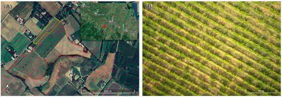
Figure 1.
(A) Experimental site (17.1 ha) located in the Forlì municipality (Emilia-Romagna, Italy). The red line and the yellow line delimit the portions of investigated vineyard cultivated, respectively, with red grapes (Sangiovese and Alicante) and white grapes (Chardonnay). (B) Aerial image of a portion of the vineyard; the plot is characterized by an average inter-row distance of 2.2 m and an average spacing between plants of 0.8 m.
The investigated 17.1 ha vineyard is primarily cultivated with Sangiovese, a red grape variety that dominates the plantation. In addition, there are smaller sections allocated for the cultivation of Alicante (red) and Chardonnay (white) grape varieties (Figure 1A), the latter covering only 1.4 ha. The vineyard is characterized by a layout with an average spacing between rows set at 2.2 m while the average distance between individual plants within a row is approximately 0.8 m (Figure 1B), leading to a plant density of ~5600 plants/ha.
2.2. Data Acquisition
The airborne survey was performed employing the Radgyro (Figure 2A), an aircraft specifically designed and manufactured for environmental investigations in the fields of radioactivity monitoring [21,22,23,24], soil mapping [25] and precision agriculture [26]. The equipment used for the acquisitions included a Sony α 7R IV Mirrorless Full-Frame photogrammetric camera (Figure 2B), configured in a nadiral position to guarantee the maximum quality of the frames collected. This camera, equipped with a 35 mm lens and a 61.0 megapixels resolution CMOS sensor, allowed the fine details of the vegetation to be captured. Georeferencing of the frames was ensured through a GNSS system (GPS, GLONASS, Galileo, BeiDou) and radar altimeter, which permits reaching positioning accuracy of the sub-meter level [27]. The achieved positioning accuracy is appropriate for the intended purpose, as it provides farmers with sufficiently accurate information to effectively locate and identify diseased plants in the vineyard.
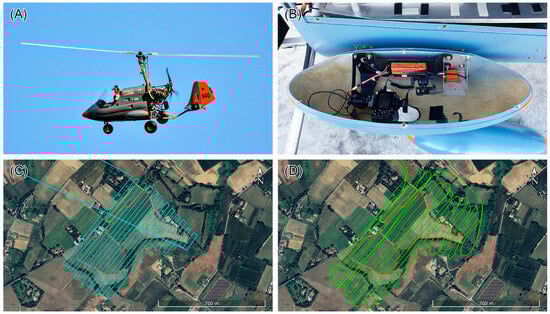
Figure 2.
(A) Radgyro, the aircraft used for the airborne photogrammetric survey. (B) The camera and independent alimentation system installed in the lateral compartment of the Radgyro. (C) Flight plan and (D) flight path of the survey performed in the study area. The red and yellow lines delimit the portions of investigated vineyard cultivated, respectively, with red grapes and white grapes.
The vineyard of the experimental site was surveyed with a single flight on the 8th of August 2023 in good weather conditions and on a sunny day. The choice of date is linked to the appearance of the first symptoms of FD in the area, which occurred in late July during the 2023 season. The flight plan was designed with an average line spacing of 25 m and complete coverage of the study area (Figure 2C) in about 17 min. The mean height and mean velocity of the realized flight (Figure 2D) were, respectively, 96 m and 73 km/h. The flight parameters permitted the reach of an average ground resolution of 1.1 cm/pixel, an overlap between two consecutive images of more than 65%, and an overlap between adjacent images of more than 70%. Before the flight, radiometric calibration was performed using a dedicated calibration panel. This procedure, which includes white balance adjustment, helps minimize the effects of illumination variability and atmospheric interference, ensuring accurate color reproduction. Nevertheless, the use of normalized vegetation indices (see Section 2.3) further mitigates the impact of varying illumination and environmental conditions, enhancing the robustness of the analysis. The resulting 1015 photograms acquired were processed to generate a georeferenced orthomosaic of the experimental site (Figure 3) with a resolution of 1.1 cm × 1.1 cm.
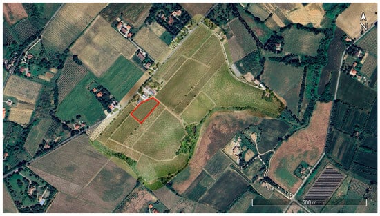
Figure 3.
Georeferenced orthomosaic derived from the processing of the photograms acquired during the airborne survey performed in the study area. The red line indicates the sample parcel used for the identification and testing of the vegetation indices (see Section 2.3).
2.3. Data Processing
To detect the plants exhibiting grapevine yellows and EC symptoms through leaf color variations, an automatic analysis process has been developed. This process relies on calculating spectral indices derived from Red (R), Green (G), and Blue (B) spectral regions combinations. A sample parcel of the experimental site (Figure 3), cultivated with red grapes, was selected for identifying and testing these indices; diseased plants were visually recognized, and their spectral response in the RGB spectral region was analyzed.
Traditionally, the Green–Red Vegetation Index (GRVI) has been used as a biomass indicator [28]:
where and are, respectively, the reflectance value of the G (500–565 nm) and R (625–750 nm) spectral regions. The GRVI is proved to be particularly effective in this context by distinguishing reflectance values in the green and red spectral regions, with a typical range from −0.2 to 0.5. Higher values are indicative of healthy plants with a lush biomass, whereas lower values suggest less vitality, as seen in dry plants [29,30].
However, after a series of tests on artificially modified images, it became clear that relying on the GRVI alone to distinguish diseased leaves from other elements such as shadows and man-made structures (e.g., cables and poles) proved inadequate, as chromatic aberrations and glare in photographs further exacerbate these differentiation challenges. To overcome this limitation, inspired by the concept of GRVI, two new indices were developed: the Green–Blue Vegetation Index (GBVI) and the Blue–Red Vegetation Index (BRVI). These indices combine reflectance in the green–blue and blue–red spectral regions, respectively:
where is the reflectance value of the B (450–485 nm) spectral region.
These indices are designed to enhance the detection of specific color changes in plant foliage: the GBVI is particularly effective in identifying variations in the green and blue wavelengths, while the BRVI focuses on the differences between the blue and red spectral regions. The performed tests demonstrated that these indices are highly effective in highlighting the reddening and yellowing of plant leaves, which are key indicators of grapevine yellows and EC symptoms.
Thanks to automatic scanning of the values of the RGB spectral indices calculated for each pixel of the sample parcel, threshold values were identified to discriminate symptomatic from healthy plants. A trial-and-error procedure helped to define, for each index, the following range to identify symptomatic plants: [GRVI < −0.08]; [GBVI > 0.35]; and [BRVI < −0.42].
To fully automate the process, a software pipeline (Figure 4) was devised with the red grape variety portion of the georeferenced orthomosaic serving as the input. This system extracts the R, G, and B reflectance values from the entire orthomosaic to calculate the three specific vegetation indices matrices. Upon simultaneously applying the predefined thresholds, the binary matrix is obtained by assigning the unit value to the pixels which passed the three threshold filters (Figure 5A–C), and the zero value to the remaining pixels. A convolution process utilizing an all-ones kernel panning across the entire binary matrix aids in noise reduction and signal isolation [31]. The noise manifests itself in the binary matrix as isolated pixels or pixel blocks that dimensionally do not represent leaves and are therefore considered irrelevant information. Consequently, noise removal is an essential step to obtain reliable results for the identification of plants with potential FD symptoms. The convolution process involves the application of a 25 pixels × 25 pixels (27.5 cm × 27.5 cm) kernel, corresponding to an area of approximately 756 cm2, to the binary matrix, with the aim of capturing details at the level of the vine leaves. A denoised binary matrix is derived, wherein a value of one is preserved only at locations where the convolution output exceeded a specific threshold. The applied threshold value of 180 pixels, corresponding to ~30% of the kernel area, allows for the removal of pixels clusters with an area smaller than 218 cm2 attributable to noise and not signal due to the leaves with potential symptoms of grapevine yellows or EC. The final output is a denoised binary matrix distinguished in pixels valued as “symptomatic” (i.e., surviving pixels) and as “healthy”.
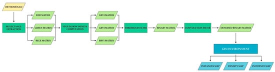
Figure 4.
Software pipeline elaborated for automating the process analysis. The input is the georeferenced orthomosaic from which the Red (R), Green (G), and Blue (B) reflectance values are extracted and used to compute the vegetation indices matrices. After the application of the threshold filters, the matrices are classified to obtain a binary matrix. The convolution filter is adopted to obtain the denoised matrix employed to produce the thematic layers in a GIS environment.
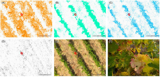
Figure 5.
(A) Green–Red Vegetation Index (GRVI), (B) Green–Blue Vegetation Index (GBVI), and (C) Blue–Red Vegetation Index (BRVI) matrices: the colored pixels are within the threshold values identified (GRVI < −0.08; GBVI > 0.35; and BRVI < −0.42). (D) Binary matrix with the pixels in black resulting from the application of the three threshold filters, (E) portion of the same area in the orthomosaic, and (F) portion of the row corresponding to the red circle which identifies the surviving pixels in the denoised matrix denoting the presence of potential disease symptoms.
The software pipeline, from the R, G, and B extraction to the production of the denoised binary matrix (Figure 4), was conducted on a PC with a 3.8 GHz Intel Core i7-10700K CPU (Intel, Canta Clara, CA, USA) and an NVIDIA GeForce GTX 1660 graphics processing unit (NVIDIA, Santa Clara, CA, USA).
The denoised binary matrix obtained by the analysis was processed in a GIS environment to produce three thematic layers: the instances map, the density map, and the incidence map (Figure 4). The elaboration of these maps aims to synthesize the analysis results and present them as products providing an immediate view of the distribution entity of the disease.
The instances map is obtained through grid resampling: the data points of the initial matrix are recalculated and assigned to a new binary grid with a cell size of 2.5 m × 2.5 m (i.e., 227 × 227 pixels). The output cell value is either 1 (“positive”), if it contains at least one surviving pixel, or 0 (“negative”). The newly defined cells on the grid, called “Prediction Boxes” (PBs), were determined to encompass an average of 3 plants. The rationale behind the specific dimensions of the PB reflects the characteristics of the vineyard plot, such as the inter-row distance of 2.2 m, but also accounts for the spatial accuracy attainable through acquisition and orthomosaic processing. Furthermore, it is important to note that the choice to communicate results at this level of resolution is deemed highly sufficient for the end user’s needs. The critical objective is not to pinpoint which specific branch or leaf manifests symptoms of disease but rather to accurately identify the presence of disease within a plant or a particular area within a row. This approach ensures that the essential information is conveyed effectively, focusing on the detection of symptomatic plants or row portions, which is both necessary and sufficient for practical purposes in intervention strategies considering the rapid spread of grapevine yellows.
Further resampling was applied to produce the density map and the incidence map, which both have a spatial resolution of 10 m × 10 m. The choice of this mesh arises from the necessity to communicate a useful and functional result for ordering and effecting compulsory mitigation measures. The disease incidence in an area of 100 m2 is indeed a crucial parameter that the regional plant protection service of the Emilia-Romagna region adopts to monitor the FD occurrence across the years and to guide decisions for the prevention of the disease diffusion. The value of each cell of the density map is the number of contained positive PBs, i.e., with diseased instances. Considering that each 10 m × 10 m contains 16 PBs and, on average, approximately 48 grapevine plants, the incidence map is classified as the percentage of the boxes with diseased instances.
To assess the spatial structure prior to statistical testing, the global spatial autocorrelation of symptomatic PBs was evaluated using Moran’s I index, which quantifies clustering relative to a null hypothesis of spatial randomness [32,33]. Statistical significance was assessed via z-scores and p-values. Based on the spatial patterns revealed by this analysis, PB-positive cells were grouped into six buffer classes reflecting an increasing distance from vineyard boundaries. This classification enabled the investigation of spatial trends in PB distribution, accounting for the edge effect, a recurrent phenomenon in studies on the epidemiology of grapevine yellows [34,35]. Given the binary nature of the data, indicating the presence or absence of positive PBs within each 10 × 10 m cell, and its skewed, zero-inflated distribution, the Kruskal–Wallis non-parametric test was applied to assess whether positive PB occurrence differed significantly across distance classes [36]. To further examine differences in PB-positive cell proportions between specific buffer pairs, a Fisher’s exact test was conducted using 2 × 2 contingency tables [37]. This approach, particularly suited for categorical and unbalanced datasets, is widely adopted in viticultural studies to explore associations between symptom presence and environmental or agronomic variables [38].
3. Results
The input orthomosaic (1.24 · 109 pixels) was processed to obtain the denoised binary matrix in a total computing time of ~65 min. Applying only one index between the GRVI, GBVI, and BRVI with the previously identified threshold’s values ([GRVI < −0.08]; [GBVI > 0.35]; and [BRVI < −0.42]) would have resulted in the selection of 26% of the pixels for the GRVI, 17% of the pixels for the GBVI, and 8% of the pixels for the BRVI (first, second, and third rows of Table 1). The simultaneous application of the three filters instead resulted in the selection of just 0.4% of the input pixels (fourth row of Table 1), with the convolution filter reducing this percentage even more (0.001% of the orthomosaic input pixels, fifth row of Table 1).

Table 1.
Number of input and output pixels for each matrix resulting from the software pipeline. For the GRVI, GBVI, and BRVI matrices the filtered pixels have values <−0.08, >0.35, and <−0.42, respectively. The filtered pixels of the binary matrix (i.e., the input pixels of the denoised binary matrix) passed all three threshold filters simultaneously. The application of the convolution filter selected the pixels of the denoised binary matrix.
The resampling of the denoised binary matrix originated the instances map with 2.73 · 104 PBs with zero value (“healthy”); the 99 PBs with value one (“symptomatic”) contains anywhere from 1 to 265 surviving pixels (Figure 6A). Half of the PBs contain less than 20 surviving pixels (~24 cm2) and only 5% contains more than 180 surviving pixels (~218 cm2).
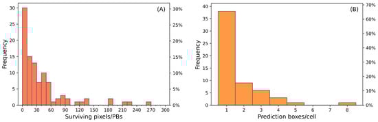
Figure 6.
(A) Frequency distribution of the surviving pixels in the Prediction Boxes (PBs) of the instances map. (B) Frequency distribution of the PBs, with at least 1 surviving pixel, in the 10 m × 10 m cells of the density and instances map.
The density and incidence maps, obtained from further resampling to 10 m × 10 m, contain 1488 cells with healthy PBs. The remaining 58 cells contain anywhere from one to eight symptomatic PBs, where most of the cells (66%) contain only one symptomatic PB (Figure 6B).
The thematic maps obtained from the processing of the data reveal that the investigated vineyard exhibits a sparse and confined presence of symptomatic plants. These findings highlight that this site is not in a critical situation regarding the general spread of grapevine yellows.
In detail, the maps show that the higher prevalence of positive PBs is recorded in two limited portions of the vineyard (Figure 7A), specifically in the northeastern (Figure 7B) and in the western areas (Figure 7D); more sparse and limited occurrences are present in the southwest (Figure 7C). The observation of low infection rates at scattered points could be indicative of primary infections, which typically occur in case of boundary infections due to incoming infected vectors [39]. This evidence could suggest performing additional monitoring activity to the surrounding vineyards with the aim of confining the further spread of grapevine yellows in the area.
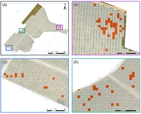
Figure 7.
Instances map: (A) entire vineyard, (B) northeastern, (C) southwestern, and (D) western subareas. Each grid cell of 2.5 m × 2.5 m represents a Prediction Box (PB) with 0 (gray cells) or at least 1 surviving pixel (colored cells).
An analysis of the density map (Figure 8A) reveals that the problematic zones have a maximum density of 6–8 PBs (equivalent to approximately 38–50 m2) (Figure 8B), while the rest of the areas exhibit lower density values (1–3 PBs, 7–19 m2) (Figure 8C). The higher density values, translating into a maximum incidence rate between 26% and 50%, are confined to small areas in the northeast (Figure 9A,B); conversely, the western area, where there is a more homogeneous distribution of predicted symptomatic plants, records density values that are almost always below 10% (Figure 9C). Higher values (11–25%) are observed in more circumscribed areas in the southwest (Figure 9D). This detailed observation underscores the spatial variability of the disease’s impact within the vineyard, highlighting specific areas where disease management efforts could be more intensely focused.
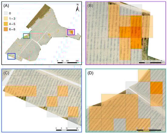
Figure 8.
Density map of the Prediction Boxes (PBs): (A) entire vineyard, (B) northeastern, (C) southwestern, and (D) western subareas. Each grid cell of 10 m × 10 m, including 16 PBs, is classified on the basis of the number of PBs with at least one surviving pixel.
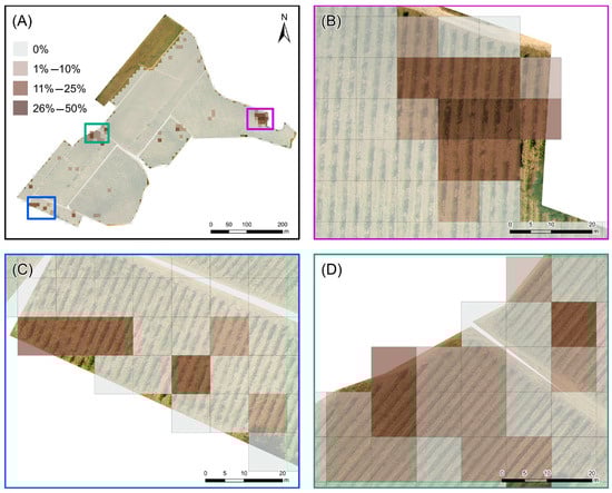
Figure 9.
Incidence map of the Prediction Boxes (PBs): (A) entire vineyard, (B) northeastern, (C) southwestern, and (D) western subareas. Each cell of the 10 m × 10 m grid includes 16 PBs and is classified according to the percentage of PBs within the cell containing at least one surviving pixel indicative of disease symptoms.
Edge effects were investigated by analyzing the spatial distribution of 10 × 10 cells with positive PBs to determine whether proximity to vineyard borders influences the occurrence of symptoms. Spatial autocorrelation analysis was used to assess the presence of clustering and to identify the optimal spatial scale for evaluating this relationship. Incremental spatial autocorrelation revealed that spatial correlation peaked at 20 m, which was adopted as the basis for defining buffer classes. The global Moran’s I index (I = 0.396, z-score = 38.19, and p-value < 0.0001) confirmed a significant clustering of symptomatic PBs, indicating deviation from spatial randomness.
Accordingly, the vineyard area was segmented into six concentric buffer zones, each 20 m wide and progressively extending inward from the vineyard borders (Figure 10A). The relative proportion of cells with positive PBs across these buffers shows a clear decreasing trend: the highest value (7.4%) was observed within the first buffer (0–20 m), followed by a progressive reduction in subsequent zones, with no symptomatic cells detected beyond 100 m (Figure 10B). This trend supports the presence of edge effects, characterized by a declining incidence of symptoms with an increasing distance from vineyard margins.
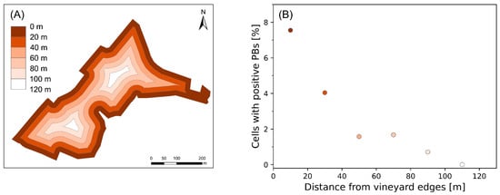
Figure 10.
(A) Spatial distribution of the six concentric buffer zones, each 20 m wide and extending inward from the vineyard edges. (B) Proportion of cells with positive PBs in each buffer class.
The Kruskal–Wallis H test, used to assess whether there were significant differences in the distributions of positive PBs among distance-based buffer groups, indicates a statistically significant difference among the groups (H = 29.764, p < 0.0001), suggesting that at least one buffer zone differs in the proportion of positive detections. To identify which pairs of buffer zones contribute the most to this difference, pairwise comparisons using the Fisher’s exact test were performed. The test analysis revealed that the 20 m buffer is significantly different from both the 60 m buffer (p = 0.0002) and the 80 m buffer (p = 0.0008), highlighting a clear decrease in detection rates with increasing distance. These comparisons confirm that the drop in positive PB presence is not due to random fluctuation but reflects a statistically meaningful spatial decay pattern. The 20 m vs. 40 m comparison also approaches significance (p = 0.0409), supporting the hypothesis of a gradient, although the difference is less pronounced. Comparisons involving the most distant buffer (120 m) were excluded from the analysis due to the very limited number of cells in this group (n = 41), which reduces test reliability.
To evaluate the performance of the developed method and its accuracy in detecting FD at the experimental site, a ground field observation campaign was conducted on the 4 October 2023. During the ground survey, expert operators detected the presence of FD, EC, and BN symptoms in the plants and recorded the spatial coordinates to compare them with the results obtained from the airborne image analysis. Due to logistical reasons, the field campaign targeted only a subset of the study area which was cultivated with the red grape variety. The subset, located in the northeastern zone (Figure 11A), contained a high number of predicted disease instances. Despite covering only 2% of the study area, the selected path allowed for the verification of about half of the instances identified by the analysis.
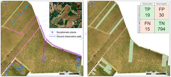
Figure 11.
The area of the experimental site investigated through the field ground observation campaign. (A) Path followed and location of the plants with observed symptoms of grapevine yellows (FD and BN) and trunk disease (EC). (B) Spatial distribution of the Prediction Boxes (PBs) resulted in agreement (TP and TN) or in disagreement (FP and FN) with the ground observations.
The ground observation path (Figure 11A) was planned to ensure the examination of the area most likely to contain diseased plants. Throughout this process, instances were verified as either true or false positives based on field observations; at the same time, observed diseased plants located in predicted boxes reported as not including symptoms in the instance map were recorded as false negatives.
To quantify the observations, a confusion matrix was constructed using a regular grid of 2.5 m × 2.5 m, covering a width of 7.5 m centered on the inspection path (Figure 11B). This grid was designed to mirror the operator’s field of view, considering both the rows of vines that were inspected directly and those adjacent, totaling four rows. The confusion matrix categories include the following [8] (Figure 11B):
- True Positive (TP = 19), representing PBs with both actual and predicted symptomatic plants;
- False Negatives (FN = 15), representing PBs with actual symptomatic plants observed in the field but not predicted;
- False Positives (FP = 30), representing PBs with predicted instances not observed in the field;
- True Negatives (TN = 794), representing PBs without symptomatic plants, aligning with both field observations and predictions.
In detail, 2 possible cases of FD or BN and 32 of EC were observed (Figure 12): 1 of the FD or BN cases was correctly identified by the analysis (TP), while among the EC cases, 17 were classified as TP and 15 as FN. This inclusion is critical due to the chromatic similarity in symptoms presented by these diseases when compared to FD. It is important to note that only molecular diagnosis can accurately differentiate FD and BN, as field observations based on visible symptoms alone may not provide the specificity necessary for distinguishing them [3].
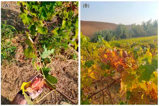
Figure 12.
Plants observed during the ground field campaign with grapevine yellows and trunk disease symptoms: (A) FD or BN and (B) EC.
The accuracy of the results obtained was quantified using the metrics, ranging between zero and one, reported in Table 2. The classification accuracy of 95% reflects the robustness of the system, with the specificity (0.96) and sensitivity (0.56) metrics suggesting that the system demonstrates an excellent capability in differentiating between healthy and symptomatic plants, and it has a good ability to identify the symptomatic plants (Table 2). The observed low Positive Predictive Value (PPV) of 0.39, attributed to the relatively high number of FP (30), suggests that the system adopts a cautious approach in the identification of symptoms associated with grapevine yellows. This conservative tendency ensures minimal risk of overlooking diseased plants but may lead to a higher rate of false alerts. On the other hand, the high Negative Predictive Value (NPV) of 0.98 reflects the system’s outstanding performance in confirming the absence of disease, indicating a robust ability to identify plants that are indeed healthy.
Table 2.
Metrics adopted to compare the results obtained from the process analysis and from the ground field observations. Adopting the definition, the values are calculated on the basis of the True Negative (TN), True Positive (TP), False Negative (FN), and False Positive (FP) of the confusion matrix in Figure 11.
The frequency distribution of surviving pixels within the validated PBs, classified as TP and FP (Figure 13), mirrors the trend observed in the entire PB population (Figure 6A). The PBs detected as TP typically include between 1 and 100 surviving pixels, underscoring the algorithm’s ability to detect early signs of discoloration with high spatial resolution. In contrast, PBs with more than 100 surviving pixels, exclusively associated with FP and concentrated in the northeastern sector of the vineyard, suggest a saturation effect: the algorithm, when exposed to extensive contiguous areas of reflectance anomalies, loses its capacity to discern early, localized disease signals. These areas likely correspond to widespread stressors unrelated to early-stage yellowing, such as senescent foliage or unmanaged inter-row vegetation. Moreover, the spatial convolution kernel used in the denoising step effectively removes isolated noise without inducing systematic oversegmentation, confirming its role in enhancing detection robustness.
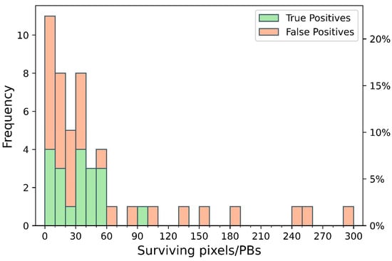
Figure 13.
Frequency distribution of surviving pixels within the Prediction Boxes (PBs) validated during the ground-truth field campaign. Bars are divided into True Positives (green), representing PBs correctly matching symptomatic vines in the field, and False Positives (red), referring to PBs not associated with any confirmed symptoms.
4. Discussion
Grapevine yellows (FD and BN) and trunk disease (EC), with their rapid spread and severe potential damage in vineyards in European regions, e.g., Emilia-Romagna (Italy), are a major concern for grape producers. While visual inspections in the field combined with sample collection remain the primary approaches for disease monitoring, these methods are often time-consuming, costly, and impractical for covering extensive vineyard areas.
Remote sensing using UAVs, aircraft, or satellites supports large-scale disease detection [40] but has certain limitations. UAVs present notable constraints such as their limited battery life, which restricts flight autonomy and the total area that can be covered during a single mission [41,42]. Similarly, the low spatial resolution of freely accessible satellite imagery (order of meters) hinders the precise differentiation between vine rows and inter-row cover crops and requires extensive pre-processing and calibration, while persistent cloud cover often causes data gaps, limiting the effectiveness of satellite-based monitoring [43,44,45]. In this pilot study, an airborne survey of a 17-hectare red grape vineyard was completed in a 17 min flight, a task that would have required approximately ten days for manual inspection, demonstrating the efficiency and scalability of aerial surveys in disease surveillance.
The use of the VIS region is prioritized: the development and the synergetic use of spectral indices based on RGB spectral regions (GRVI, GBVI, and BRVI) showed good efficacy in identifying symptomatic plants comparable to traditional field methods. Firstly, RGB imagery offers a spatial resolution at least an order of magnitude greater than NIR. Additionally, the RGB analysis mimics the agronomist’s field approach, where yellows and reds are identified based on a visible spectrum observation.
Generally, hyperspectral imaging offers detailed spectral information for disease detection, but the large data volumes require extensive computational resources [20] impeding their scalability and efficiency in real-world viticultural contexts. In this sense, Ref. [17] emphasized the need for efficient pipelines to process hyperspectral high-resolution UAV data. Machine learning algorithms, such as convolutional neural networks and support vector machines, amplify processing requirements due to the need to train on large inputs. Indeed, deep learning models often risk overfitting on limited data, reducing their generalizability [18,46], and their high computational requirements demand costly hardware. Recently, feature selection methods like genetic algorithms [18], dimensionality reduction and noise filtering [47,48] have attempted to address these limitations. In contrast, the proposed RGB approach can be calibrated using just a single sample parcel, significantly reducing the time and resources needed. The automated analysis processed the 1.24 · 109 pixels of the orthomosaic in 65 min, identifying 99 prediction 2.5 m × 2.5 m boxes as showing signs of disease.
The spatial distribution of symptoms revealed a marked edge effect, with a significantly higher occurrence near vineyard edges. This finding was supported by spatial autocorrelation metrics and confirmed by statistical tests (Kruskal–Wallis and Fisher’s exact test), indicating a non-random, distance-dependent pattern of symptom presence. This spatial pattern is consistent with previous studies, which identified the vineyard border, particularly those adjacent to herbaceous vegetation such as nettle, as primary sources of phytoplasma inoculum due to the higher density of grapevine yellows vectors, typically found along these edges.
The accuracy of the results of the proposed method is evaluated, with an ad hoc ground-based survey, in terms of overall accuracy (0.95) and specificity (0.96) comparable to the best-performing methods in different studies. For instance, in Ref. [18], the highest classification accuracy of 0.96 was achieved using genetic algorithm features with a logistic regression classifier, while a slightly lower accuracy of 0.85 was obtained with ensemble-selected features. Ref. [14] achieved an accuracy exceeding 0.96 using the best model combination of the successive projection algorithm, vegetation indices, support vector machine, and discriminant analysis specifically tailored to grapevine varieties. Similarly, Ref. [15] reported the highest specificity values (0.99) using a Vegetation Index-based approach; lower values (0.71–0.92) were obtained using different methods based on single spectral bands or biophysical parameters. In addition to the variability in specificity, they obtained sensitivity values ranging from 0.46 to 1.0 depending on the method used, highlighting the variability of results across different approaches. In contrast, our method yielded a lower sensitivity value of 0.56, suggesting room for improvement in detecting symptomatic plants. To address this limitation and enhance model performance, a threshold-based exclusion of saturated PBs could be implemented to reduce FP. This strategy relies on the identification of PBs overly affected by non-specific spectral responses, such as those induced by severe vegetative stress unrelated to disease symptoms (e.g., senescent leaves or dense inter-row weeds). The precise detection of such saturation patterns would require the development of deep learning models trained on datasets enriched with representative examples of these conditions. Nevertheless, the overall performance of our approach, particularly in terms of specificity, remains competitive, reinforcing its potential in disease surveillance within vineyards. A dedicated study was conducted to evaluate how changes in threshold values of spectral indices and the convolution filter affect the accuracy evaluation. The pipeline analysis was repeated by adopting threshold values within the ranges defined for the sample parcel (GRVI < [−0.10; −0.07]; GBVI > [0.32; 0.35]; and BRVI < [−0.42; −0.40]) with steps of 0.01. The maximum variability observed in the computed TP, FP, FN, and FP leads to a value of 0.92 for the specificity and 0.38 for the sensitivity. Additionally, the effect of varying the convolution filter threshold (from 20% to 40% of the kernel area) on FN detection was tested while keeping the spectral indices constant. Lowering the threshold to 20% did not affect TP or FN detection but markedly increased FP (116), reducing specificity to 0.86. Conversely, increasing the threshold to 40% reduced FP to 8, but drastically decreased TP (4) and increased FN (30), resulting in a sensitivity of only 0.12.
It is important to note that the 57-day lag between airborne and ground surveys (due to logistical reasons related to field operations and beyond our control) could have implications on the results obtained. Symptoms of grapevine yellows and EC become more visible over time, possibly causing the ground survey to detect cases not visible in the earlier airborne survey and explaining the FN occurrences. A similar temporal effect was observed in Ref. [14], where two acquisition campaigns conducted in early August, when symptoms were not yet fully visible, and the second in September, during the late growing season, revealed a significant increase in symptom visibility in the latter phase.
The inability of airborne surveys to distinguish between FD, BN, and EC due to overlapping symptoms limits disease management strategies. While EC symptoms are easily recognizable during the visual survey, BN and FD share visual symptoms like leaf discoloration and reddening, making their discrimination very challenging in remote sensing-based detection. In such cases, laboratory analyses (e.g., molecular analysis) become essential to confirm the presence of phytoplasma within the plant [8,18,46,49]. Despite this limitation, airborne surveys offer significant advantages by providing rapid and comprehensive spatial coverage, enabling the early identification of potential problem areas across large vineyard plots. Additionally, the high-resolution data collected can support strategic planning and resource allocation. Complementing airborne surveys with targeted field inspections strengthens early detection and minimizes economic losses from false positive eradications [40].
This approach paves the way for the development of an early warning system, significantly impacting viticulture by providing growers with a powerful tool for disease management, ultimately leading to healthier vineyards and improved grape quality [50]. Looking forward, the next step is to apply this approach (i.e., airborne acquisitions and the automated analysis method) on larger areas and other varieties of red grapes, thus validating their generalizability in different environmental and cultural contexts.
Our airborne imaging system can survey up to 60 hectares of vineyards per hour. The Forlì-Cesena province, covering 2377 km2, hosts approximately 5000 highly scattered vineyards with an average size of 1.2 ha, resulting in a highly scattered spatial distribution, posing a significant monitoring challenge.
Moreover, the method has the potential to be applied to satellite image datasets with sufficient resolution to investigate vineyards details, offering a scalable solution for monitoring larger geographical areas and different crop types [51,52].
5. Conclusions
This work presents a pilot study about the use of high-resolution airborne imaging for the detection of grapevine yellows (Flavescence dorée and Bois Noir) and trunk disease (Esca Complex) in a vineyard in Emilia-Romagna (Italy). The primary objective was to develop a cost-effective and automated methodology for the early detection of grapevine disease in vineyards utilizing airborne-acquired RGB imagery, thereby eliminating the reliance on costly multispectral and hyperspectral sensors.
The chosen flight parameters successfully provided images with a high spatial resolution, marking a crucial step in the methodological framework. Given the centimetric resolution required to discern symptoms, the analysis outputs—instance, density, and incidence maps—stress the necessity of consolidating results to effectively communicate findings, guiding actionable measures. These thematic maps reveal detailed views of the spatial distribution of grapevine disease, facilitating focused and strategic field interventions. The identification of isolated cases, potentially indicative of primary infections and difficult to detect through ground surveys, is critical in preventing the spread of diseases to unaffected areas. Benefitting from these findings, farmers and specialized technicians can focus their time-consuming ground inspections on areas where symptomatic plants have been identified, providing strategic direction for monitoring these symptomatic zones. In addition, the integration of spatial autocorrelation metrics and statistical testing confirmed the presence of edge effects, highlighting a significant relationship between symptom occurrence and proximity to vineyard borders, an aspect to be considered in both surveillance strategies and disease containment planning
By offering an accessible and scalable monitoring tool, this study contributes to the advancement of sustainable viticulture, enabling efficient disease mapping and early-stage detection, facilitating real-time decision-making in vineyard management. Furthermore, this research serves as a preliminary step toward designing a systematic approach for future aerial surveys aimed at the large-scale targeting of disease detection and management with the aim of providing a comprehensive evaluation of the method’s robustness and applicability under diverse environmental conditions, phenological stages, and grape varieties.
Author Contributions
Conceptualization, V.S., F.M. (Fabio Mantovani) and K.G.C.R.; Data curation, M.A., E.C. and A.M.; Formal analysis, M.A., A.M. and K.G.C.R.; Funding acquisition, V.S., S.B., T.C., E.G. and F.M. (Fabio Mantovani); Investigation, V.S., M.A., L.C., E.C., N.I.E., A.M., F.M. (Fabio Mantovani) and F.M. (Federica Migliorini); Methodology, V.S., M.A., S.B., L.C., R.C., A.M., F.M. (Fabio Mantovani), F.M. (Federica Migliorini), K.G.C.R. and R.T.; Project administration, V.S. and F.M. (Fabio Mantovani); Resources, A.B., T.C., F.G., E.G., N.L., F.M. (Filippo Mantovani), D.P. and S.P.; Software, G.H., V.S., E.C., A.M., F.M. (Filippo Mantovani) and K.G.C.R.; Supervision, V.S., S.B., L.C., F.M. (Fabio Mantovani), F.M. (Federica Migliorini) and R.T.; Validation, V.S., M.A., S.B., L.C., A.M., F.M. (Fabio Mantovani), F.M. (Federica Migliorini), K.G.C.R. and R.T.; Visualization, V.S., G.G., A.M., F.M. (Fabio Mantovani) and K.G.C.R.; Writing—original draft, V.S. and K.G.C.R.; Writing—review and editing, V.S., M.A., A.B., S.B., L.C., E.C., R.C., T.C., N.I.E., G.G., F.G., E.G., G.H., N.L., A.M., F.M. (Fabio Mantovani), G.L.M., F.M. (Federica Migliorini), D.P., S.P., K.G.C.R. and R.T. All authors have read and agreed to the published version of the manuscript.
Funding
This research was funded by the project PERBACCO (Early warning system per la PrEvenzione della diffusione della flavescenza doRata BAsato sul monitoraggio multiparametriCo airborne delle COlture vinicole) (CUP E47F23000030002) funded by the Emilia-Romagna Region. The work is partially funded by (i) the ICSC—Centro Nazionale di Ricerca in High Performance Computing, Big Data and Quantum Computing, funded by European Union—NextGenerationEU—CUP F77G22000120006, and (ii) the “GeoneUtrinos: mESSengers of the Earth’s interior” (GUESS) project funded by European Union—NextGenerationEU—CUP F53D23001280006.
Data Availability Statement
The data that supports the findings of this study are available from the corresponding author, V.S., upon reasonable request.
Acknowledgments
The authors express their gratitude to the “Club Aeronautico Sassuolo” and Vassalli Bakering for their valuable support and cooperation, and thank Mauro Antongiovanni, Claudio Pagotto, Angelo Montalti, Adriano Facchini, and Flavia Dorelli for the fruitful discussions.
Conflicts of Interest
The authors declare no conflicts of interest.
References
- Oliveira, M.J.R.A.; Castro, S.; Paltrinieri, S.; Bertaccini, A.; Sottomayor, M.; Santos, C.S.; Vasconcelos, M.W.; Carvalho, S.M.P. “Flavescence dorée” impacts growth, productivity and ultrastructure of Vitis vinifera plants in Portuguese “Vinhos Verdes” region. Sci. Hortic. 2020, 261, 108742. [Google Scholar] [CrossRef]
- Chuche, J.; Thiéry, D. Biology and ecology of the Flavescence dorée vector Scaphoideus titanus: A review. Agron. Sustain. Dev. 2014, 34, 381–403. [Google Scholar] [CrossRef]
- Belli, G.; Bianco, P.A.; Conti, M. Grapevine yellows in Italy: Past, present and future. J. Plant Pathol. 2010, 92, 303–326. [Google Scholar]
- Bertaccini, A.; Vibio, M.; Stefani, E. Detection and molecular characterization of phytoplasmas infecting grapevine in Liguria (Italy). Phytopathol. Mediterr. 1995, 34, 137–141. [Google Scholar]
- Mori, N.; Cargnus, E.; Martini, M.; Pavan, F. Relationships between Hyalesthes obsoletus, Its Herbaceous Hosts and Bois Noir Epidemiology in Northern Italian Vineyards. Insects 2020, 11, 606. [Google Scholar] [CrossRef]
- Cruz, A.; Ampatzidis, Y.; Pierro, R.; Materazzi, A.; Panattoni, A.; De Bellis, L.; Luvisi, A. Detection of grapevine yellows symptoms in Vitis vinifera L. with artificial intelligence. Comput. Electron. Agric. 2019, 157, 63–76. [Google Scholar] [CrossRef]
- Graniti, A.; Mugnai, L.; Surico, G. Esca of Grapevine: A Disease Complez or a Complex of Diseases. Phytopathol. Mediterr. 2000, 39, 16–20. [Google Scholar]
- Daglio, G.; Cesaro, P.; Todeschini, V.; Lingua, G.; Lazzari, M.; Berta, G.; Massa, N. Potential field detection of Flavescence dorée and Esca diseases using a ground sensing optical system. Biosyst. Eng. 2022, 215, 203–214. [Google Scholar] [CrossRef]
- Mondello, V.; Songy, A.; Battiston, E.; Pinto, C.; Coppin, C.; Trotel-Aziz, P.; Clement, C.; Mugnai, L.; Fontaine, F. Grapevine Trunk Diseases: A Review of Fifteen Years of Trials for Their Control with Chemicals and Biocontrol Agents. Plant Dis. 2018, 102, 1189–1217. [Google Scholar] [CrossRef]
- Terentev, A.; Dolzhenko, V.; Fedotov, A.; Eremenko, D. Current State of Hyperspectral Remote Sensing for Early Plant Disease Detection: A Review. Sensors 2022, 22, 757. [Google Scholar] [CrossRef]
- Zhang, J.; Huang, Y.; Pu, R.; Gonzalez-Moreno, P.; Yuan, L.; Wu, K.; Huang, W. Monitoring plant diseases and pests through remote sensing technology: A review. Comput. Electron. Agric. 2019, 165, 104943. [Google Scholar] [CrossRef]
- Oerke, E.-C. Remote Sensing of Diseases. Annu. Rev. Phytopathol. 2020, 58, 225–252. [Google Scholar] [CrossRef]
- Al-Saddik, H.; Simon, J.-C.; Cointault, F. Development of Spectral Disease Indices for ‘Flavescence Dorée’ Grapevine Disease Identification. Sensors 2017, 17, 2772. [Google Scholar] [CrossRef]
- Al-Saddik, H.; Simon, J.C.; Cointault, F. Assessment of the optimal spectral bands for designing a sensor for vineyard disease detection: The case of ‘Flavescence dorée’. Precis. Agric. 2018, 20, 398–422. [Google Scholar] [CrossRef]
- Albetis, J.; Duthoit, S.; Guttler, F.; Jacquin, A.; Goulard, M.; Poilvé, H.; Féret, J.-B.; Dedieu, G. Detection of Flavescence dorée Grapevine Disease Using Unmanned Aerial Vehicle (UAV) Multispectral Imagery. Remote Sens. 2017, 9, 308. [Google Scholar] [CrossRef]
- Naidu, R.A.; Perry, E.M.; Pierce, F.J.; Mekuria, T. The potential of spectral reflectance technique for the detection of Grapevine leafroll-associated virus-3 in two red-berried wine grape cultivars. Comput. Electron. Agric. 2009, 66, 38–45. [Google Scholar] [CrossRef]
- Gatou, P.; Tsiara, X.; Spitalas, A.; Sioutas, S.; Vonitsanos, G. Artificial Intelligence Techniques in Grapevine Research: A Comparative Study with an Extensive Review of Datasets, Diseases, and Techniques Evaluation. Sensors 2024, 24, 6211. [Google Scholar] [CrossRef]
- Imran, H.A.; Zeggada, A.; Ianniello, I.; Melgani, F.; Polverari, A.; Baroni, A.; Danzi, D.; Goller, R. Low-Cost Handheld Spectrometry for Detecting Flavescence Dorée in Vineyards. Appl. Sci. 2023, 13, 2388. [Google Scholar] [CrossRef]
- Hruška, J.; Adão, T.; Pádua, L.; Guimarães, N.; Peres, E.; Morais, R.; Sousa, J.J. Evaluation of machine learning techniques in vine leaves disease detection: A preliminary case study on flavescence dorée. Int. Arch. Photogramm. Remote Sens. Spat. Inf. Sci. 2019, XLII-3/W8, 151–156. [Google Scholar] [CrossRef]
- Feng, L.; Wu, B.; Zhu, S.; He, Y.; Zhang, C. Application of Visible/Infrared Spectroscopy and Hyperspectral Imaging with Machine Learning Techniques for Identifying Food Varieties and Geographical Origins. Front. Nutr. 2021, 8, 680357. [Google Scholar] [CrossRef]
- Strati, V.; Baldoncini, M.; Bezzon, G.P.; Broggini, C.; Buso, G.P.; Caciolli, A.; Callegari, I.; Carmignani, L.; Colonna, T.; Fiorentini, G.; et al. Total natural radioactivity, Veneto (Italy). J. Maps 2015, 11, 545–551. [Google Scholar] [CrossRef]
- Baldoncini, M.; Alberi, M.; Bottardi, C.; Minty, B.; Raptis, K.G.C.; Strati, V.; Mantovani, F. Airborne Gamma-Ray Spectroscopy for Modeling Cosmic Radiation and Effective Dose in the Lower Atmosphere. IEEE Trans. Geosci. Remote Sens. 2018, 56, 823–834. [Google Scholar] [CrossRef]
- Baldoncini, M.; Albéri, M.; Bottardi, C.; Minty, B.; Raptis, K.G.C.; Strati, V.; Mantovani, F. Exploring atmospheric radon with airborne gamma-ray spectroscopy. Atmos. Environ. 2017, 170, 259–268. [Google Scholar] [CrossRef]
- Raptis, K.G.C.; Albéri, M.; Bisogno, S.; Callegari, I.; Chiarelli, E.; Cicala, L.; Colonna, T.; De Cesare, M.; Guastaldi, E.; Maino, A.; et al. External effective dose from natural radiation for the Umbria region (Italy). J. Maps 2022, 18, 461–471. [Google Scholar] [CrossRef]
- Maino, A.; Alberi, M.; Anceschi, E.; Chiarelli, E.; Cicala, L.; Colonna, T.; De Cesare, M.; Guastaldi, E.; Lopane, N.; Mantovani, F.; et al. Airborne Radiometric Surveys and Machine Learning Algorithms for Revealing Soil Texture. Remote Sens. 2022, 14, 3814. [Google Scholar] [CrossRef]
- Finco, A.; Bentivoglio, D.; Chiaraluce, G.; Alberi, M.; Chiarelli, E.; Maino, A.; Mantovani, F.; Montuschi, M.; Raptis, K.G.C.; Semenza, F.; et al. Combining Precision Viticulture Technologies and Economic Indices to Sustainable Water Use Management. Water 2022, 14, 1493. [Google Scholar] [CrossRef]
- Alberi, M.; Baldoncini, M.; Bottardi, C.; Chiarelli, E.; Fiorentini, G.; Raptis, K.G.C.; Realini, E.; Reguzzoni, M.; Rossi, L.; Sampietro, D.; et al. Accuracy of Flight Altitude Measured with Low-Cost GNSS, Radar and Barometer Sensors: Implications for Airborne Radiometric Surveys. Sensors 2017, 17, 1889. [Google Scholar] [CrossRef]
- Yin, G.; Verger, A.; Descals, A.; Filella, I.; Peñuelas, J. A Broadband Green-Red Vegetation Index for Monitoring Gross Primary Production Phenology. J. Remote Sens. 2022, 2022, 9764982. [Google Scholar] [CrossRef]
- Motohka, T.; Nasahara, K.N.; Oguma, H.; Tsuchida, S. Applicability of Green-Red Vegetation Index for Remote Sensing of Vegetation Phenology. Remote Sens. 2010, 2, 2369–2387. [Google Scholar] [CrossRef]
- Bendig, J.; Yu, K.; Aasen, H.; Bolten, A.; Bennertz, S.; Broscheit, J.; Gnyp, M.L.; Bareth, G. Combining UAV-based plant height from crop surface models, visible, and near infrared vegetation indices for biomass monitoring in barley. Int. J. Appl. Earth Obs. Geoinf. 2015, 39, 79–87. [Google Scholar] [CrossRef]
- Jiang, Y.; Wronski, B.; Mildenhall, B.; Barron, J.T.; Wang, Z.; Xue, T. Fast and High Quality Image Denoising via Malleable Convolution. In Computer Vision—ECCV 2022; Lecture Notes in Computer Science; Springer: Berlin/Heidelberg, Germany, 2022; pp. 429–446. [Google Scholar]
- Moran, P.A. Notes on continuous stochastic phenomena. Biometrika 1950, 37, 17–23. [Google Scholar] [CrossRef] [PubMed]
- Matese, A.; Di Gennaro, S.F.; Santesteban, L.G. Methods to compare the spatial variability of UAV-based spectral and geometric information with ground autocorrelated data. A case of study for precision viticulture. Comput. Electron. Agric. 2019, 162, 931–940. [Google Scholar] [CrossRef]
- Mori, N.; Pavan, F.; Bondavalli, R.; Reggiani, N.; Paltrinieri, S.; Bertaccini, A. Factors affecting the spread of “Bois Noir” disease in north Italy vineyards. Vitis 2008, 47, 65. [Google Scholar]
- Pavan, F.; Mori, N.; Bigot, G.; Zandigiacomo, P. Border effect in spatial distribution of Flavescence dorée affected grapevines and outside source of Scaphoideus titanus vectors. Bull. Insectol. 2012, 65, 281–290. [Google Scholar]
- Kruskal, W.H.; Wallis, W.A. Use of Ranks in One-Criterion Variance Analysis. J. Am. Stat. Assoc. 1952, 47, 583–621. [Google Scholar] [CrossRef]
- Fisher, R.A. On the Interpretation of χ2 from Contingency Tables, and the Calculation of P. J. R. Stat. Soc. 1922, 85, 87–94. [Google Scholar] [CrossRef]
- Calzarano, F.; Di Marco, S.; D’Agostino, V.; Schiff, S.; Mugnai, L.J.P.M. Grapevine leaf stripe disease symptoms (esca complex) are reduced by a nutrients and seaweed mixture. Phytopathol. Mediterr. 2014, 53, 543–558. [Google Scholar]
- Maggi, F.; Bosco, D.; Galetto, L.; Palmano, S.; Marzachi, C. Space-Time Point Pattern Analysis of Flavescence Doree Epidemic in a Grapevine Field: Disease Progression and Recovery. Front. Plant Sci. 2016, 7, 1987. [Google Scholar] [CrossRef]
- Portela, F.; Sousa, J.J.; Araujo-Paredes, C.; Peres, E.; Morais, R.; Padua, L. A Systematic Review on the Advancements in Remote Sensing and Proximity Tools for Grapevine Disease Detection. Sensors 2024, 24, 8172. [Google Scholar] [CrossRef]
- Pádua, L.; Matese, A.; Di Gennaro, S.F.; Morais, R.; Peres, E.; Sousa, J.J. Vineyard classification using OBIA on UAV-based RGB and multispectral data: A case study in different wine regions. Comput. Electron. Agric. 2022, 196, 106905. [Google Scholar] [CrossRef]
- Torres-Sanchez, J.; Mesas-Carrascosa, F.J.; Santesteban, L.G.; Jimenez-Brenes, F.M.; Oneka, O.; Villa-Llop, A.; Loidi, M.; Lopez-Granados, F. Grape Cluster Detection Using UAV Photogrammetric Point Clouds as a Low-Cost Tool for Yield Forecasting in Vineyards. Sensors 2021, 21, 3083. [Google Scholar] [CrossRef]
- Mucalo, A.; Matić, D.; Morić-Španić, A.; Čagalj, M. Satellite Solutions for Precision Viticulture: Enhancing Sustainability and Efficiency in Vineyard Management. Agronomy 2024, 14, 1862. [Google Scholar] [CrossRef]
- Crespo, N.; Pádua, L.; Santos, J.A.; Fraga, H. Satellite Remote Sensing Tools for Drought Assessment in Vineyards and Olive Orchards: A Systematic Review. Remote Sens. 2024, 16, 2040. [Google Scholar] [CrossRef]
- Williams, M.; Burnside, N.G.; Brolly, M.; Joyce, C.B. Investigating the Role of Cover-Crop Spectra for Vineyard Monitoring from Airborne and Spaceborne Remote Sensing. Remote Sens. 2024, 16, 3942. [Google Scholar] [CrossRef]
- Boulent, J.; St-Charles, P.L.; Foucher, S.; Theau, J. Automatic Detection of Flavescence Doree Symptoms Across White Grapevine Varieties Using Deep Learning. Front. Artif. Intell. 2020, 3, 564878. [Google Scholar] [CrossRef] [PubMed]
- García-Vera, Y.E.; Polochè-Arango, A.; Mendivelso-Fajardo, C.A.; Gutiérrez-Bernal, F.J. Hyperspectral Image Analysis and Machine Learning Techniques for Crop Disease Detection and Identification: A Review. Sustainability 2024, 16, 6064. [Google Scholar] [CrossRef]
- Carneiro, G.A.; Cunha, A.; Aubry, T.J.; Sousa, J. Advancing Grapevine Variety Identification: A Systematic Review of Deep Learning and Machine Learning Approaches. AgriEngineering 2024, 6, 4851–4888. [Google Scholar] [CrossRef]
- Pavan, F.; Cargnus, E.; Frizzera, D.; Martini, M.; Ermacora, P. Interactions between bois noir and the esca disease complex in a Chardonnay vineyard in Italy. Phytopathol. Mediterr. 2024, 63, 303–314. [Google Scholar] [CrossRef]
- Bendel, N.; Kicherer, A.; Backhaus, A.; Kluck, H.C.; Seiffert, U.; Fischer, M.; Voegele, R.T.; Topfer, R. Evaluating the suitability of hyper- and multispectral imaging to detect foliar symptoms of the grapevine trunk disease Esca in vineyards. Plant Methods 2020, 16, 142. [Google Scholar] [CrossRef]
- Johnson, L.F.; Roczen, D.E.; Youkhana, S.K.; Nemani, R.R.; Bosch, D.F. Mapping vineyard leaf area with multispectral satellite imagery. Comput. Electron. Agric. 2003, 38, 33–44. [Google Scholar] [CrossRef]
- Zhou, X.; Yang, L.; Wang, W.; Chen, B. UAV Data as an Alternative to Field Sampling to Monitor Vineyards Using Machine Learning Based on UAV/Sentinel-2 Data Fusion. Remote Sens. 2021, 13, 457. [Google Scholar] [CrossRef]
Disclaimer/Publisher’s Note: The statements, opinions and data contained in all publications are solely those of the individual author(s) and contributor(s) and not of MDPI and/or the editor(s). MDPI and/or the editor(s) disclaim responsibility for any injury to people or property resulting from any ideas, methods, instructions or products referred to in the content. |
© 2025 by the authors. Licensee MDPI, Basel, Switzerland. This article is an open access article distributed under the terms and conditions of the Creative Commons Attribution (CC BY) license (https://creativecommons.org/licenses/by/4.0/).