VJDNet: A Simple Variational Joint Discrimination Network for Cross-Image Hyperspectral Anomaly Detection

Abstract

To enhance the generalization of networks and avoid redundant training efforts, cross-image hyperspectral anomaly detection (HAD) based on deep learning has been gradually studied in recent years. Cross-image HAD aims to perform anomaly detection on unknown hyperspectral images after a single training process on the network, thereby improving detection efficiency in practical applications. However, the existing approaches may require additional supervised information or stacking of networks to improve model performance, which may impose high demands on data or hardware in practical applications. In this paper, a simple and lightweight unsupervised cross-image HAD method called Variational Joint Discrimination Network (VJDNet) is proposed. We leverage the reconstruction and distribution representation ability of the variational autoencoder (VAE), learning the global and local discriminability of anomalies jointly. To integrate these representations from the VAE, a probability distribution joint discrimination (PDJD) module is proposed. Through the PDJD module, the VJDNet can directly output the anomaly score mask of pixels. To further facilitate the unsupervised paradigm, a sample pair generation module is proposed, which is able to generate anomaly samples and background representation samples tailored for the cross-image HAD task. The experimental results show that the proposed method is able to maintain the detection accuracy with only a small number of parameters.

1. Introduction

Hyperspectral images typically consist of hundreds of continuous spectral bands, usually ranging from visible to mid-infrared [1,2]. Due to the rich information contained in the high spectral dimension, hyperspectral images can sensitively distinguish different landforms and objects according to their materials [3,4]. Therefore, hyperspectral images are often used to discover anomalies in scenes, such as airplanes, tanks, or other objects in backgrounds like airports or forests [5]. The task of identifying anomalous objects from hyperspectral backgrounds is called hyperspectral anomaly detection (HAD), which has a wide range of practical applications [6,7].

For HAD, a major challenge is that the prior information of anomalies is usually unknown, and therefore it is usually regarded as an unsupervised task [8,9]. Moreover, there are several characteristics between anomalies and the backgrounds in hyperspectral images [10]. Anomalous targets are usually composed of materials such as metal, plastic, and paint, occupying a small proportion in remote sensing scenes, with spectral characteristics that differ significantly from the environment (soil, vegetation, cement, water, etc.). Based on these characteristics, many statistics-based methods were proposed in early research [11,12,13]. The Reed–Xiaoli (RX) detector is one of the most classic methods [14]. It assumes that the background follows a multivariate Gaussian distribution and detects anomalies by calculating the Mahalanobis distance between the central pixel and surrounding pixels. Subsequently, some improved RX detectors were proposed, such as the local RX [15] and the kernel RX algorithm [16].

However, for complex regions, the background may not be accurately estimated with statistical models. To remove such limitations, many other methods have been proposed, such as representation-based methods and tensor decomposition-based methods [17,18,19,20]. Collaborative representation detection (CRD) [21] is a representation-based method that assumes a background pixel can be represented by its surrounding pixels while anomalous pixels cannot. Methods based on low-rank and sparse representation (LRASR) exploit the low-rank characteristics of the background [22,23]. In order to further model background and anomaly information, an HAD method based on potential anomaly and background dictionary construction (PAB-DC) was proposed [24]. Shen et al. [25] introduced the saliency prior and utilized framelet decomposition to maintain the sparsity and piecewise smoothness of background representation. Total variation regularization is also commonly used in tensor-based HAD methods due to its ability to maintain piecewise smoothness [26,27]. Feng et al. [28] combined tensor ring decomposition with TV regularization, exploiting both the low-rank property and piecewise smoothness in the spatial and spectral dimensions. These methods achieve good detection performance through the representation and decomposition of hyperspectral images. However, for different hyperspectral images, different dictionaries and representations need to be constructed, making the parameters difficult to apply in unknown hyperspectral images.

In recent years, with the rapid development of deep neural networks, numerous deep learning-based HAD methods have been proposed, such as deep belief network (DBN) [29], convolutional neural network (CNN) [30,31], generative adversarial network (GAN) [10,32], long short-term memory (LSTM) [33], and autoencoder (AE) [34,35]. Many methods utilize AEs to reconstruct hyperspectral images and distinguish anomalies from the background through reconstruction errors. These methods are usually based on an assumption that the number of anomalous pixels is significantly smaller than the number of backgrounds. Therefore, the model tends to learn the reconstruction criterion of the background, while anomalies cannot be reconstructed well [36,37,38]. By introducing a convolutional autoencoder, Wang et al. proposed Auto-AD [39], reconstructing hyperspectral images from random noise. Gao et al. proposed a blind-spot architecture that uses surrounding pixels to reconstruct the central pixel, thereby suppressing the reconstruction of anomalies [40,41]. Liu et al. introduced enhanced separation training to address the identical mapping problem in the reconstruction process [42,43]. Cheng et al. [9] introduced an alternating optimization strategy to reduce the effects of anomalies during optimization. Wu et al. [44] proposed a Transformer-based autoencoder that enhances the representation of global spatial information. Liu et al. [45] combined low-rank representation models with self-supervised learning, using deep neural networks to generate pseudo-anomalies. Chen et al. [46] proposed a spectral diffusion model to further infer the potential background of the anomalous regions. Variational autoencoders (VAEs) have also been used in anomaly detection in recent years [47]. The VAE implements regularization constraints on the encoded latent space features, so it can obtain latent space features with regular distribution, thereby reducing the overfitting of the model. Lei et al. [5] introduced the VAE into HAD, leveraging the strong representation capability of the VAE to extract inherent spectral features from high-dimensional spectral vectors. Subsequently, some improved methods were introduced to the VAE to further enhance HAD performance, such as 3D convolution [48], graph regularization [49], manifold learning, and multi-head self-attention [50]. Yu et al. [51], combining the Chebyshev neighborhood, discriminated anomalies based on the latent layer probability distribution of pixels. Since the latent layer constraint can reduce the interference of anomalous samples on learning background reconstruction, the variational inference method was also introduced into a GAN to obtain hyperspectral image reconstruction in a generative strategy [52].

These deep learning methods mostly learn from a single hyperspectral image in an unsupervised manner and detect anomalies in the current image. They require training a specific network for each hyperspectral image, and the knowledge learned from one hyperspectral image is difficult to extend to other images. Therefore, the detection efficiency is likely to be reduced. To address these issues, in recent years, many studies have begun exploring HAD across images. Li et al. used a CNN to learn the similarity between pixels and their surroundings through classification labels and discriminated if the central pixel is anomalous [30]. Based on relation learning, Huyan et al. [53] introduced VLAD pooling to project different image features into the same space. Li et al. [54] first proposed an unsupervised cross-image HAD model that can directly generate an anomaly map in one step. Ma et al. [55] proposed a statistical offset module that enables the model to adapt to hyperspectral images in different domains. To extract spatial context information, AETNet was proposed, which can learn reconstruction rules directly from a set of hyperspectral images [56]. As shown in Figure 1, these cross-image HAD methods do not need to be optimized for each unknown image. However, the current cross-image HAD methods still face the following issues.

(1)

Knowledge transfer misalignment. During the model training process, additional supervised information may be required, such as classification labels. However, the background may contain various categories of land cover in HAD, which might be classified as negative samples in category classification, thereby affecting the performance of the model.

(2)

Implicit modeling. The existing cross-image HAD methods mostly learn features of background and anomalies in an implicit manner, insufficiently considering the distribution differences between the background and anomalies for reconstruction or discrimination.

(3)

High computational complexity. In order to maintain performance, most existing cross-image HAD methods require stacking of networks, such as CNNs or Transformers, resulting in extensive parameters and hardware requirements.

To address the above issues, a simple and lightweight cross-image HAD model is proposed in this paper. Like other cross-image HAD methods, once it is trained, for any new image, only one forward propagation is required to obtain the detection map without additional optimization. Based on the assumption that background pixels in hyperspectral images are much more than anomalies, we use artificially generated anomalies and original pixels to train a binary classification network to perform HAD without ground truth labels. After sampling from the central pixel and the surrounding pixels, through a model based on a siamese VAE, the VJDNet can combine global and local information to discriminate anomalies. From the global perspective, by learning the probability of pixels being reconstructed, the model can identify anomalies with low reconstruction probability from the whole image, which are difficult to be reconstructed. To prevent the model from overfitting to specific images, we use a relatively broad reconstruction probability rather than the precise spectral angle distances as the learning objective. From the local perspective, by encoding the distributions of pixels and their surroundings, the model can identify anomalies that are significantly different from the surrounding pixels based on local information. To integrate global and local information, we propose a probability distribution joint discrimination (PDJD) module, which can directly obtain the anomaly score of the input pixels. Furthermore, we propose generating methods for anomaly samples and surrounding background representations, respectively, considering the stability and cross-image generalization of the generated samples. For anomaly samples, we generate them through dynamic weights to ensure their diversity and difference from the original pixels. On the other hand, in the original image, the surrounding pixels might contain anomalous pixels. Therefore, we establish a distribution for the surrounding pixels and sample from it to obtain representations. Compared with the existing cross-image HAD methods, the proposed VJDNet can be implemented with just a few fully connected layers, making it highly lightweight while maintaining good detection performance and scalability. The main contributions of this paper can be summarized as follows.

(1)

A lightweight cross-image HAD network based on a siamese VAE named VJDNet is proposed. The network is able to learning global and local distributions from samples of multiple hyperspectral images and detect anomalies in unknown hyperspectral images after one unsupervised training process. Compared with other advanced unsupervised cross-image HAD methods, our proposed method achieves comparable or even superior performance while utilizing a lightweight network structure.

(2)

A probability distribution joint discriminant (PDJD) module is proposed, which can simultaneously consider reconstruction probabilities and distribution differences to distinguish anomalies. The PDJD module can combine the information of the pixel itself and the information of the surroundings to achieve more accurate anomaly detection.

(3)

We propose a dynamic sample pair generation strategy. This generative module balances the stability and randomness of training samples, allowing the model to learn more diverse representations and better adapt to unknown hyperspectral images.

• The remainder of this paper is organized as follows. Section 2 provides a brief overview of the related works covered in this paper, specifically introducing VAEs and cross-image HAD. Section 3 provides a detailed explanation of the proposed method. Section 4 presents the experimental results and analysis, validating the effectiveness of the proposed method. Finally, a conclusion is given in Section 5.

2. Related Work

2.1. Variational Autoencoder

The variational autoencoder (VAE) is an encoder–decoder-structured network that can be used for generation tasks [57]. Its difference from the autoencoder (AE) is that AE learns reconstruction from sample to sample, while the VAE aims to learn probability distributions. Given a sample $\mathbf{x}$, the VAE assumes that it can be generated from an unobservable continuous random variable $\mathbf{z}$. To learn this generation process, the model aims to maximize a posterior probability $p_{\theta }\left(\mathbf{x}\right|\mathbf{z})$ that conforms to a multivariate Gaussian distribution, where $\theta$ represents the parameters of the decoder. To obtain the latent variable $\mathbf{z}$, the posterior probability $q_{\varphi }\left(\mathbf{z}\right|\mathbf{x})$ is computed by the encoder, where $\varphi$ represents the parameters of the encoder. In order to ensure the generation ability and prevent degeneration into an ordinary AE, the VAE usually uses a KL divergence as the latent layer constraint to make the distribution of $q_{\varphi }\left(\mathbf{z}\right|\mathbf{x})$ close to the prior probability of the latent variable $p_{\theta }\left(\mathbf{z}\right)$. Finally, the VAE can be trained by maximizing the evidence lower bound (ELBO). For each data point ${\mathbf{x}}_i$, ELBO is defined as

$$\mathcal{L}(\theta ,\varphi ;{\mathbf{x}}_i)=E_{q_{\varphi }\left(\mathbf{z}\right|{\mathbf{x}}_i)}[log{p}_{\theta }\left({\mathbf{x}}_i\right|\mathbf{z})]-\mathbb{KL}\left(q_{\varphi }\left(\mathbf{z}\right|{\mathbf{x}}_i)\parallel p_{\theta }\left(\mathbf{z}\right)\right)$$

(1)

Generally, the standard normal distribution $\mathcal{N}(0,\mathbf{I})$ is used as the prior probability distribution. Consequently, for each sample $\mathbf{x}$, the VAE can encode it into a multivariate distribution approximating the standard normal distribution. By sampling from the distribution in the latent space, the VAE can generate new samples with a similar distribution to the input sample.

For anomaly detection tasks, the posterior probability $p_{\theta }\left(\mathbf{x}\right|\mathbf{z})$ generated by the decoder can be used to represent the probability of a pixel being reconstructed in the hyperspectral image, thus serving as the anomaly score [47,51]. Some other works use mean squared error loss (MSE) and spectral angle loss (SAD) instead of reconstruction probabilities to facilitate efficient post-processing [5]. In this paper, due to its good robustness and generalization, we design the cross-image HAD method based on the VAE and explore its joint representation and discriminative capabilities between different hyperspectral images.

2.2. Cross-Image Hyperspectral Anomaly Detection

In the past two years, cross-image hyperspectral anomaly detection (HAD) has become prominent among researchers. In previous studies, most deep learning-based HAD methods were trained and tested on the same hyperspectral image. That is, for each hyperspectral image, an individual model needs to be trained. This results in the need to store a large number of parameters when dealing with a large number of hyperspectral images. Consequently, cross-image HAD methods have been gradually explored. However, there are differences in scenes or sensors between hyperspectral images, which is a significant challenge for cross-image HAD.

The earliest methods introduced pixel-level classification labels, learning whether pixels are similar based on their categories and those of their surroundings [30]. This approach simplified anomaly detection into a binary classification task of “similar” or “dissimilar” between pixels, making the model easier to transfer. Based on this idea, AUD-Net introduces VLAD pooling to project pixels of different images to the same space [53]. In addition, a memory module was proposed to predict the feature of the central pixel through surrounding features. Pixels that are difficult to predict have a greater probability of being anomalous. These methods have verified the effectiveness of cross-image HAD. However, they all require the introduction of additional classification labels, which means there are still limitations on the data. Ma et al. proposed an unsupervised background suppression model and designed a statistical offset module that enables the model to generalize to other images [55]. However, it relies on existing HAD methods such as RX for detection. The Transferred Direct Detection (TDD) model [54] and Anomaly Enhancement Transformation Network (AETNet) [56] are both unsupervised HAD methods. The TDD model simulates and constructs some anomalies in the image, allowing the model to learn discriminative features using the labels of these “anomalies”. On the other hand, AETNet overlays masks on the image, causing the model to reconstruct the covered parts from surrounding pixels. Through this approach, the model will reconstruct anomalous pixels as background during the implementation, resulting in reconstruction errors. Most of these existing cross-image HAD methods require stacking large networks to achieve good performance. Therefore, we conduct research from the perspectives of local distribution and global reconstruction probability, aiming to design a lightweight cross-image HAD model with good performance.

3. Methodology

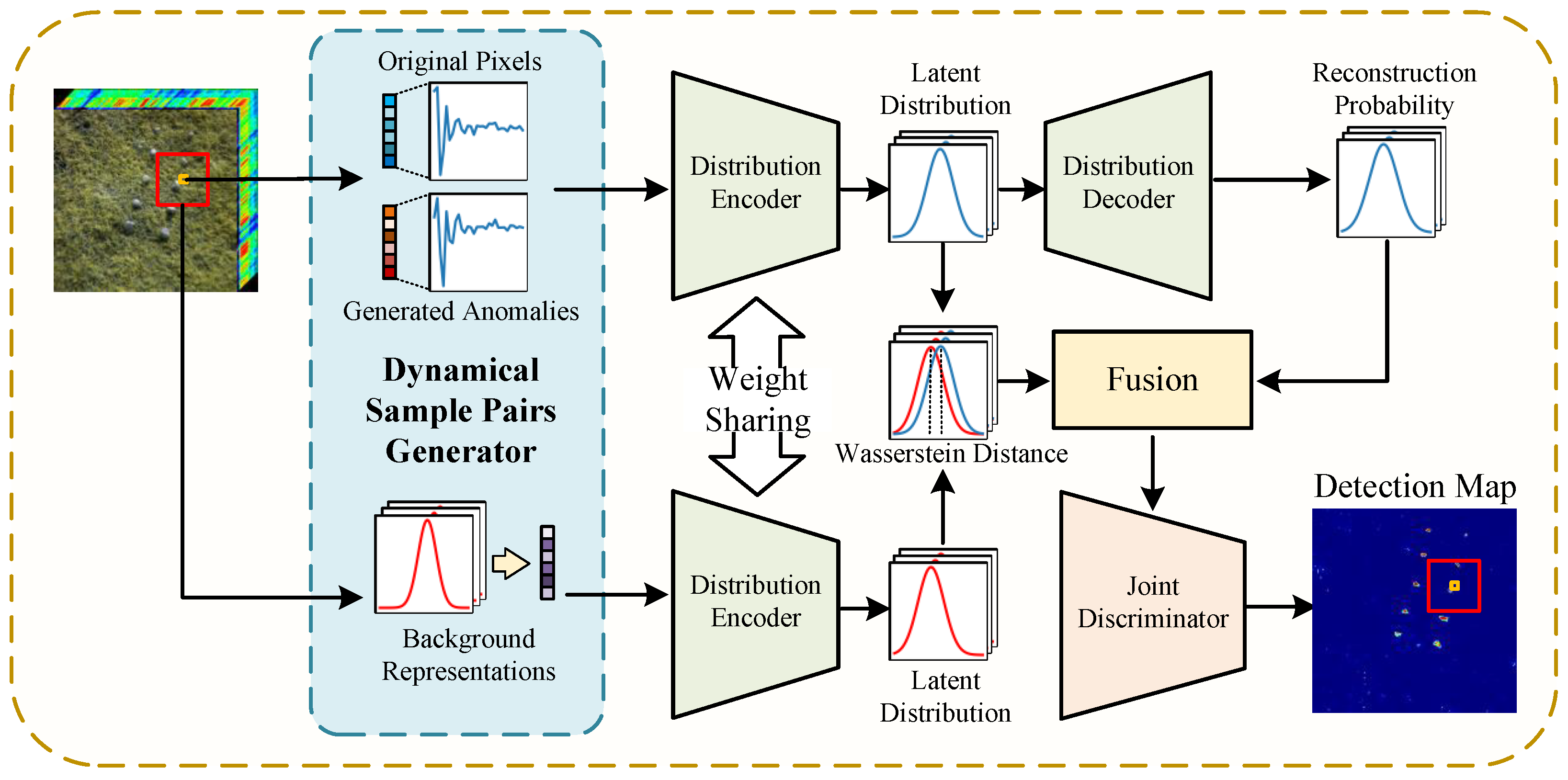
In this paper, we propose a siamese variational autoencoder (VAE)-based cross-image hyperspectral anomaly detection model, named Variational Joint Discrimination Network (VJDNet). After training with multiple hyperspectral images, the VJDNet can perform anomaly detection on other hyperspectral images not involved in the training process. The overall structure of the VJDNet is shown in Figure 2. It mainly consists of three parts: sample pair generation module, siamese VAE module, and probability-distribution joint discrimination (PDJD) module. First, the VJDNet dynamically constructs a series of background–center pixel sample pairs. The background representation is extracted by dual windows and resampled according to the distribution model, while the central pixel mutates into an anomaly according to a preset probability. After obtaining such sample pairs, we use two weight-shared VAEs to represent their latent distribution and the reconstruction probability of the central pixel. Finally, the PDJD module combines the reconstruction probability of the central pixel and the difference in latent distribution between the background and central pixels to determine whether the central pixel is an anomaly.

3.1. Dynamical Generation of Sample Pairs

In the sample pair generation module, we first divide the input hyperspectral image into image patches according to the dual window sizes $w_{in}$ and $w_{out}$. For the model to learn discriminative features between anomalies and non-anomalies, we need to mutate the central pixel to an anomaly based on a preset probability $\rho$. Then, we model the distribution of surrounding pixels between the inner and outer windows and sample representative surrounding background pixels from the modeled distribution.

Given N image patches, $\mathcal{P}={\left\{{\mathbf{P}}_i\right\}}_{i=1}^N\in {\mathbb{R}}^{w_{out}\times w_{out}\times c}$, which may come from different hyperspectral images, where c is the spectral dimension after dimensionality reduction. In this work, we use principal component analysis (PCA) to reduce the dimension of hyperspectral images and achieve dimensional unification between images. Each image patch ${\mathbf{P}}_i$ contains two elements, the central pixel $x_c$ and the surrounding pixel set $\mathbf{x}={\left\{x_j\right\}}_{j=1}^{N_s}$. $N_s$ represents the number of surrounding pixels, which can be calculated from the double window size as follows:

$$N_s=w_{out}^2-w_{in}^2$$

(2)

For the central pixel $x_c$, we generate anomalies based on the probability $\rho$. That is, in one anomaly generation process, each central pixel has a $\rho$ probability of being selected as an anomaly. Anomalies can be generated by shuffling the spectral order of the original pixels [54]. However, for samples after PCA dimension reduction, shuffling the dimensions may destroy the data structure at the level of feature space. Therefore, we have designed an anomaly generation method by generating weight vectors. Once a pixel is selected, a random weight array ${\mathit{w}}_a$ is generated according to Gaussian distribution $\mathcal{N}(1,\mathbf{I})$, in which the negative value is fixed to 1. Then, the selected center pixel is multiplied by ${\mathit{w}}_a$. As a result, the values in some dimensions of generated anomalies remain unchanged, while the values in the remaining dimensions are randomly enlarged or reduced, resulting in features different from the original pixels. This approach is able to generate anomalies similar to the original pixels in some dimensions, thus constraining the decision boundary by similar but not identical samples rather than significantly different samples, enhancing the discriminability of the model. After we obtain the center pixel $x_c$, the corresponding binary label y is also generated. When $y=1$, it means that the corresponding center pixel $x_c$ is selected as the generated anomaly. On the contrary, when $y=0$, the center pixel $x_c$ remains unchanged, and it is regarded as a normal sample.

For the surrounding pixel set $\mathbf{x}$, we first model its distribution. Many previous works have assumed that the background of hyperspectral images can be represented by a multivariate Gaussian distribution. Due to the double window, the surrounding pixels are limited to a smaller scope, so their distribution is generally closer than that of the global image. Therefore, we model $\mathbf{x}$ as a univariate Gaussian distribution $\mathcal{N}({\mu }_s,{\sigma }_s^2)$ on each reduced spectral dimension, where

$${\mu }_s={\displaystyle \frac{1}{N_s}}\sum _{j=1}^{N_s}{x}_j$$

(3)

$${\sigma }_s=\sqrt{{\displaystyle \frac{1}{N_s}}\sum _{j=1}^{N_s}{(x_j-{\mu }_s)}^2}$$

(4)

We perform $N_b$ sampling in the distribution $\mathcal{N}({\mu }_s,{\sigma }_s^2)$ to obtain the sampled background pixels and then take their mean as the background representation $x_b$ of the image patch. This approach makes $x_b$ representative and close to the mean value of surrounding pixels while also introducing some randomness to enhance the network’s generalization and resistance to interference. To make the trained model more adaptable for transfer between images, we use a dynamic approach where anomaly and background generation are performed once per training epoch. This approach enriches the diversity of samples and reduces the overfitting of the model on training hyperspectral images.

During the inference stage, we use the mean ${\mu }_s$ of the surrounding pixels as the background representation. This is because the inference process is only performed once, so, compared to the training process, it is necessary to reduce randomness to ensure the stability of the detection results. Since most of the background representations generated during training are close to the mean ${\mu }_s$, the model can achieve good detection performance during the inference process as well.

3.2. Model Architecture

The network structure consists of three parts: distribution encoder, distribution decoder, and probability-distribution joint discriminator. The encoder and decoder together form a VAE structure. To keep the model as lightweight as possible, we use several fully connected structures to build the network. We use Leaky ReLU as the activation layer in the model to ensure non-zero output of neurons, avoid gradient vanishing, and enhance the generalization capability of the network. It is worth noting that, during the encoding and decoding process of background representation, we fixed the parameters of the network. That is, the encoder and decoder only learn the distribution representation and reconstruction probability of the central pixel and share the weights for the forward-propagation process of the background representation. The reason is that the background representation is obtained by resampling from the background distribution, and we hope that the VAE part can maximize the reconstruction probability of real pixels as much as possible.

3.2.1. Distribution Encoder

The distribution encoder $\mathit{E}$ consists of three fully connected layers, with a Batch Normalization layer and an activation layer between every two layers. We use a siamese structure to construct the encoder, which can encode the input sample pairs into latent distribution representations separately. Therefore, the input layer size of the encoder is the same as the sample spectral size. The last layer size is twice the latent size, which is used to represent the mean value ${\mu }_l\in {\mathbb{R}}^{c_l}$ and standard deviation ${\sigma }_l\in {\mathbb{R}}^{c_l}$ of the latent distribution, where $c_l$ is the latent-layer size. The encoding process can be represented as

$$({\mu }_{lc},{\sigma }_{lc})=\mathit{E}(x_c;{\mathit{W}}_e,{\mathit{b}}_e)$$

(5)

$$({\mu }_{lb},{\sigma }_{lb})=\mathit{E}(x_b;{\mathit{W}}_e,{\mathit{b}}_e)$$

(6)

where ${\mathit{W}}_e$ and ${\mathit{b}}_e$ are the weight and bias of the encoder $\mathit{E}$, respectively. Then, the latent layer distribution $q_c$ of the center pixel and the latent layer distribution $q_b$ of the background representation can be represented as

$$q_c\left(z\right)={\displaystyle \frac{1}{{\sigma }_{lc}\sqrt{2\pi }}}{e}^{-{\displaystyle \frac{{(z-{\mu }_{lc})}^2}{2{\sigma }_{lc}^2}}}$$

(7)

$$q_b\left(z\right)={\displaystyle \frac{1}{{\sigma }_{lb}\sqrt{2\pi }}}{e}^{-{\displaystyle \frac{{(z-{\mu }_{lb})}^2}{2{\sigma }_{lb}^2}}}$$

(8)

For the latent distribution representation, we refer to the latent layer constraint of the VAE and use KL divergence as the loss function to make it close to the standard normal distribution; that is,

$$p\left(z\right)={\displaystyle \frac{1}{\sqrt{2\pi }}}{e}^{-{\displaystyle \frac{z^2}{2}}}$$

(9)

$${\mathcal{L}}_{dis}={\displaystyle \frac{1}{N}}\sum _{i=1}^N\mathbb{KL}\left(q_{ci}\left(z\right)\parallel p\left(z\right)\right)$$

(10)

3.2.2. Distribution Decoder

Similar to the encoder, the distribution decoder $\mathit{D}$ also consists of three fully connected layers, with a Batch Normalization layer and an activation layer between every two fully connected layers. Before decoding, the VAE performs M sampling from the latent distribution to obtain latent sample representations $\mathbf{z}\sim \mathcal{N}({\mu }_l,{\sigma }_l^2)$. Then, the decoder reconstructs the latent sample representations into corresponding reconstruction distributions. Therefore, the input size of the decoder is the same as the latent size, while the output size is twice the sample spectral size, used to represent the mean ${\mu }_r\in {\mathbb{R}}^c$ and the standard deviation ${\sigma }_r\in {\mathbb{R}}^c$ of the reconstruction distribution. For each latent-layer sample representation $z_k$, similar to the encoding process, the reconstruction process can be represented as

$$({\mu }_{rk},{\sigma }_{rk})=\mathit{D}(z_k;{\mathit{W}}_d,{\mathit{b}}_d)$$

(11)

where ${\mathit{W}}_d$ and ${\mathit{b}}_d$ are the weight and bias of the decoder $\mathit{D}$, respectively. Since we only use the center pixels to optimize the weights of the VAE module, the background representation does not participate in the reconstruction decoding process. Then, the reconstruction distribution $p_k$ of the central pixel can be represented as

$$p_k\left(\overline{x}\right)={\displaystyle \frac{1}{{\sigma }_{rk}\sqrt{2\pi }}}{e}^{-{\displaystyle \frac{{(\overline{x}-{\mu }_{rk})}^2}{2{\sigma }_{rk}^2}}}$$

(12)

We use the logarithmic probability of the center pixel $x_c$ in the reconstruction distribution as the reconstruction probability and take the average over the number of latent samples. The final reconstruction probability $\rho$ can be represented as

$$\rho ={\displaystyle \frac{1}{M}}\sum _{k=1}^{M}log\left[p_k\left(x_c\right)\right]$$

(13)

The objective of the VAE is to maximize the reconstruction probability; thus, the reconstruction loss can be represented as

$${\mathcal{L}}_{recon}=-{\displaystyle \frac{1}{N}}\sum _{i=1}^N{\rho }_i$$

(14)

3.2.3. Probability-Distribution Joint Discriminator

To jointly utilize the relationship between pixels with global hyperspectral images and with local surrounding pixels, we propose a probability-distribution joint discriminator (PDJD) module. First, we calculate the distance between the latent distributions of the central pixel $q_c$ and of the background representation $q_b$ to measure the difference between the central pixel and its surroundings. In this work, we use Wasserstein distance to measure the distance between latent layer distributions. Wasserstein distance measures the minimum cost of transforming one distribution into another, effectively reflecting their distance regardless of whether there is overlap between distributions. Since the dimensions are independent of each other, the distribution distance $d\in {\mathbb{R}}^{c_l}$ can be expressed as

$$d=\mathcal{W}{\left(q_c\left(z\right),q_b\left(z\right)\right)}^2=\left|\right|{\mu }_{lc}-{\mu }_{lb}{\left|\right|}_2^2+\left|\right|{\sigma }_{lc}-{\sigma }_{lb}{\left|\right|}_2^2$$

(15)

Then, the distribution distance d and the reconstruction probability $\rho$ are concatenated to obtain the joint measurement representation r. We use a classification network $\mathit{F}$ to discriminate whether the represented central pixel $x_c$ belongs to an anomaly based on the joint measurement representation. The classification network $\mathit{F}$ consists of three fully connected layers, with an activation layer between each two layers. Finally, we use a softmax layer to obtain the probability of $x_c$ being classified as background or anomaly, where the probability of being classified as anomaly can serve as the output anomaly score. We use cross-entropy loss as the classification loss ${\mathcal{L}}_{cls}$, which can be represented as

$${\mathcal{L}}_{cls}=-{\displaystyle \frac{1}{N}}\sum _{i=1}^N\left[y_{i}log\left(\mathit{F}\left(r_i\right)\right)+(1-y_i)log\left(1-\mathit{F}\left(r_i\right)\right)\right]$$

(16)

where $y_i$ is the binary classification label, indicating that the i-th sample is a background sample or a generated anomaly sample. $r_i$ is the joint measurement representation of the i-th sample. Finally, introducing a balancing parameter $\lambda$, the overall loss function of the model is

$$\mathcal{L}={\mathcal{L}}_{dis}+{\mathcal{L}}_{recon}+\lambda {\mathcal{L}}_{cls}$$

(17)

After the discriminator, we apply an n-th power operation to the output. In this work, the exponent n is set to 3 to suppress the background while keeping the integrity of the anomalous regions.

4. Experiments

4.1. Dataset Description

To verify the cross-image anomaly detection capabilities of the VJDNet, six different datasets are used in this work. Their specific details are as follows.

(1)

San Diego Dataset [22]: This dataset was collected by the Airborne Visible/Infrared Imaging Spectrometer (AVIRIS, Jet Propulsion Laboratory, Pasadena, CA, USA) sensor in San Diego, CA, USA. The original data size is $400\times 400$, with a resolution of 3.5 m per pixel, containing 224 spectral bands ranging from 400–2500 nm. For anomaly detection, 35 bands with low quality are removed, and a subset of $100\times 100$ is selected, containing 143 anomalous pixels.

(2)

Cri Dataset [58]: This dataset was collected by the Nuance Cri (PerkinElmer, Waltham, MA, USA) hyperspectral sensor, containing 46 bands ranging from 650–1100 nm. The image size is $400\times 400$, containing 1254 anomalous pixels.

(3)

HYDICE Dataset [21]: This dataset was collected by the Hyperspectral Digital Imagery Collection Experiment (HYDICE, Naval Research Laboratory, Washington, DC, USA) sensor, containing 175 bands after removing water vapor absorption bands. The image size is $80\times 100$, with 1 m per pixel as the spatial resolution. There are 21 anomalous pixels representing cars and roofs in the image.

(4)

WHU-Hi-River Dataset [59]: This dataset was collected by the Nano-Hyperspec (Headwall Photonics, Bolton, MA, USA) visible and near-infrared UAV-borne hyperspectral sensor, containing 135 bands ranging from 400 to 1000 nm. The image size is $105\times 168$, with 6 cm per pixel as the spatial resolution. There are 21 anomalous pixels representing plastic plates in the image.

(5)

Airport–Beach–Urban (ABU) Dataset [60]: This dataset contains 13 hyperspectral scenes, including airport, beach, and urban. They were collected by the AVIRIS sensor and the Reflective Optics System Imaging Spectrometer (ROSIS-03, Deutsches Zentrum für Luft- und Raumfahrt, Oberpfaffenhofen, Germany) sensor. The images are $100\times 100$ or $150\times 150$ in size, with different spatial resolutions and numbers of the spectral bands.

(6)

HAD-100 Dataset [56]: This is a large-scale hyperspectral dataset containing 260 training images and 100 test images, collected by the AVIRIS-NG sensor. The test images are $64\times 64\times 276$ in size, with spatial resolutions ranging from 1.9 m to 8.4 m.

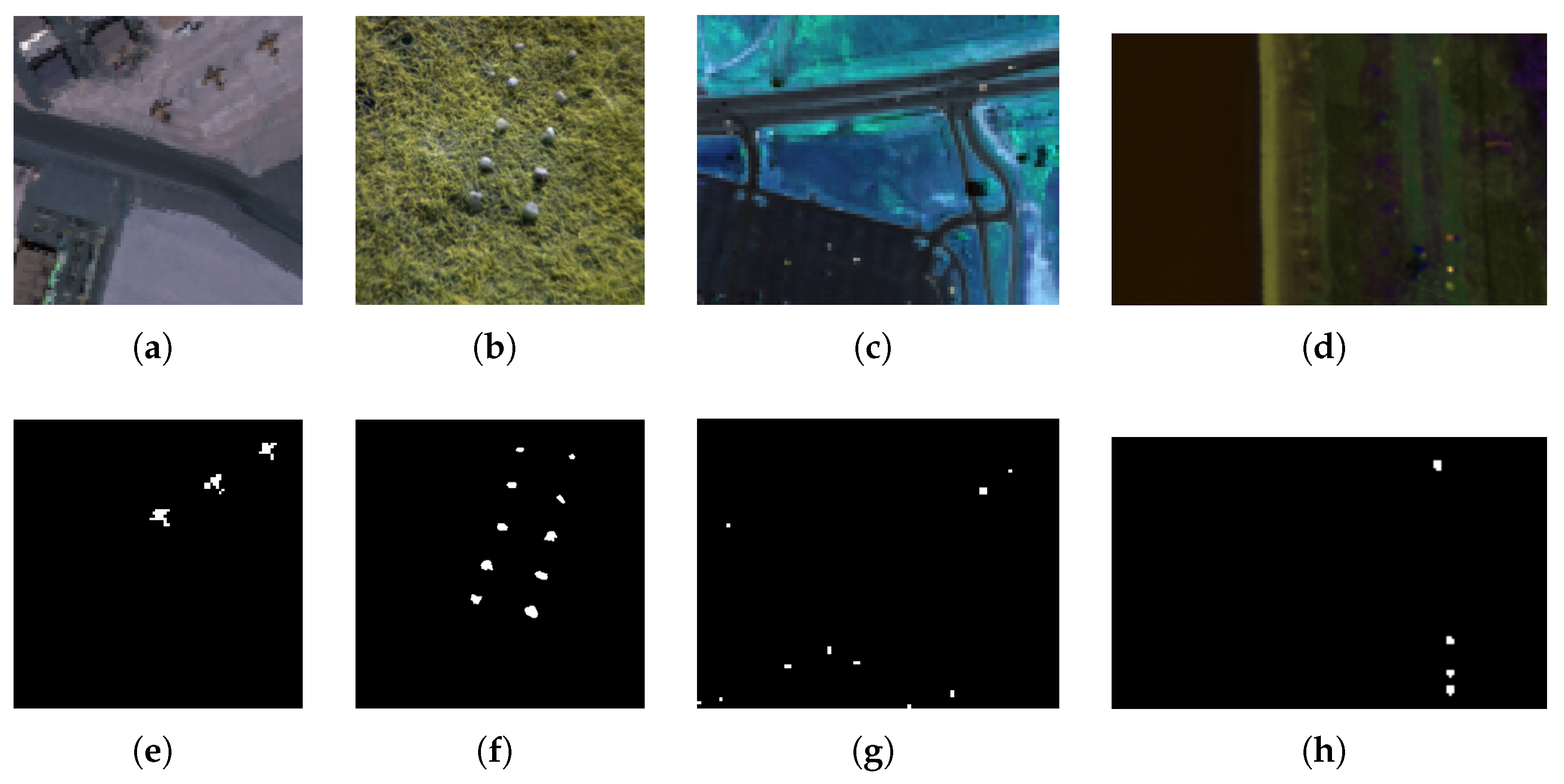
The pseudo-color images and ground truths of the four individual datasets used for testing are shown in Figure 3, and some detailed information is listed in

Table 1. Detailed information of the datasets.

Images	Sensor	Resolution	Size
San Diego	AVIRIS	3.5 m	$100\times 100\times 189$
Cri	Nuance Cri	-	$400\times 400\times 46$
HYDICE	HYDICE	1 m	$80\times 100\times 175$
WHU-Hi-River	Nano-Hyperspec	0.06 m	$105\times 168\times 135$
Airport-1	AVIRIS	7.1 m	$100\times 100\times 205$
Airport-2	AVIRIS	7.1 m	$100\times 100\times 205$
Airport-3	AVIRIS	7.1 m	$100\times 100\times 205$
Airport-4	AVIRIS	3.4 m	$100\times 100\times 191$
Beach-1	AVIRIS	17.2 m	$150\times 150\times 188$
Beach-2	AVIRIS	7.5 m	$100\times 100\times 193$
Beach-3	AVIRIS	4.4 m	$100\times 100\times 188$
Beach-4	ROSIS-03	1.3 m	$150\times 150\times 102$
Urban-1	AVIRIS	17.2 m	$100\times 100\times 204$
Urban-2	AVIRIS	17.2 m	$100\times 100\times 207$
Urban-3	AVIRIS	3.5 m	$100\times 100\times 191$
Urban-4	AVIRIS	7.1 m	$100\times 100\times 205$
Urban-5	AVIRIS	7.1 m	$100\times 100\times 205$

.

4.2. Implementation Details

In this work, the input hyperspectral images are normalized and scaled to the range [0, 1]. Then, to keep the input sample size consistent, we use principal component analysis (PCA) to reduce the spectral size to 30. In the sample pair generation module, the inner window size $w_{in}$ is set to $5\times 5$, while the outer window size $w_{out}$ is $21\times 21$. For cross-image detection, the anomaly generation probability $\rho$ is set to 0.2; for single-image detection, $\rho$ is set to 0.5. The number of background representation samples $N_b$ is 10 each time, and the number of latent-layer samples M is also set to 10. In the network, the latent size is set as 20. The balancing parameter $\lambda$ is set to 1. The whole model is trained by the Adam optimizer with a learning rate of $1\times {10}^{-6}$, and the batch size is set to 64.

For cross-image anomaly detection, we first train the VJDNet on 13 images of the ABU dataset, and then verify the detection performance on the remaining four individual datasets. To reduce the computational cost, we randomly select 3500 pixels and their surroundings from each image as training samples. Afterward, these samples are randomly shuffled and sent to the network for learning. In this way, the VJDNet achieves simultaneous training on multiple hyperspectral images. For the HAD-100 dataset, we randomly select 1000 pixels and their surroundings from each training image. After training the network, detection is performed on all images in the test set.

4.3. Comparative Methods and Evaluation Metrics

In the comparative experiment, we compared the VJDNet with 11 methods: RX [14], CRD [21], LRASR [22], 2S-GLRT [61], Auto-AD [39], GT-HAD [62], MSNet [43], CNND [30], AUD-Net [53], AET-Net [56], and BSDM [55]. Among them, RX and 2S-GLRT are statistics-based methods, while CRD and LRASR are representation-based methods. In deep learning methods, Auto-AD, MSNet, and CNND are CNN-based methods, GT-HAD and AUD-Net are Transformer-based methods, AET-Net is a method combining CNN and Transformer, and BSDM is a method based on Denoising Diffusion Probabilistic Models (DDPMs).

For Auto-AD, the experiment is conducted only on single-image detection. For cross-image detection by GT-HAD, we concatenate the training images into a large image to train the network and then perform inference on the four test images. For CNND and AUD-Net, since they require classification labels for supervised training, the experiment is conducted only for cross-image detection. We use the pre-trained weights on their default hyperspectral classification dataset for testing. For other methods, similarly to the proposed VJDNet, the hyperspectral image is first normalized, and the spectral dimension is reduced to 30 by PCA. For CRD and 2S-GLRT, the settings of the dual-window size are the same as those of the proposed VJDNet. Other experimental settings are consistent with those in the original paper.

To evaluate the performance of the model, the receiver operating characteristic (ROC) curves are plotted based on the relationship between the true positive rate $P_d$, the false positive rate $P_f$, and the threshold $\tau$. Then, their areas under the curve (AUCs) are calculated as the quantitative metric. Moreover, we also compare the number of parameters, FLOPs, and inference times of the methods to verify the lightweightness of the VJDNet.

4.4. Comparative Results on Single-Image Detection

We first verified the anomaly detection performance of the VJDNet by training and testing on the same hyperspectral images. The experimental results are shown in

Table 2. AUC($P_d$, $P_f$) for different methods of single-image detection.

Dataset	RX	CRD	LRASR	2S-GLRT	Auto-AD	GT-HAD	MSNet	AET-Net	BSDM	VJDNet
San Diego	0.9737	0.9810	0.9836	0.9745	0.9893	0.9871	0.9829	0.9660	0.9742	0.9892
Cri	0.9646	0.9558	0.8152	0.8048	0.9893	0.9960	0.9951	0.9973	0.9573	0.9926
HYDICE	0.9911	0.9941	0.9558	0.9545	0.8916	0.9640	0.9937	0.9627	0.9929	0.9878
River	0.9987	0.9978	0.8911	0.9990	0.7188	0.9896	0.9895	0.9986	0.9989	0.9952
Mean	0.9820	0.9822	0.9114	0.9332	0.8973	0.9842	0.9903	0.9812	0.9808	0.9912

, in which River is the abbreviation of the WHU-Hi-River dataset. As can be seen from the table, the proposed VJDNet does not achieve the best performance on a single dataset but shows overall balance and thus achieves the highest mean score of AUROC.

As shown in the table, CRD exhibits significant performance on the HYDICE datasets but does not perform as well on the Cri dataset. Similarly, LRASR and 2S-GLRT also perform poorly on the Cri dataset. This may be because the spectral range and dimension size of the Cri dataset are significantly different from others. On the other hand, Auto-AD achieves the best performance on the San Diego dataset but experiences a large performance drop on the WHU-Hi-River dataset. The proposed VJDNet demonstrates good detection performance on these four datasets, which have varying sensors, resolutions, and data sizes, thus showing its universality.

4.5. Comparative Results on Cross-Image Detection

4.5.1. Comparison on Four Individual Datasets

To verify the performance of the VJDNet on cross-image HAD, we compared it with different methods for cross-image detection. Among these, traditional methods such as RX, CRD, LRASR, and 2S-GLRT do not perform cross-image detection, so they have the same results as single-image detection. The CNND and AUD-Net are cross-image HAD methods based on classification labels, so they are first trained on their default classification datasets and then perform anomaly detection on the four test datasets. The remaining methods are first trained on 13 images from the ABU dataset and then tested on the four datasets. The AUC scores for each method are shown in

Table 3. AUC scores for different methods of cross-image detection on four individual datasets.

AUC(${\mathit{P}}_{\mathit{d}}$, ${\mathit{P}}_{\mathit{f}}$) ↑
Dataset	RX	CRD	LRASR	2S-GLRT	GT-HAD	MSNet	CNND	AUD-Net	AET-Net	BSDM	VJDNet
San Diego	0.9737	0.9810	0.9836	0.9745	0.9859	0.9704	0.9051	0.9533	0.9720	0.9743	0.9890
Cri	0.9646	0.9558	0.8152	0.8048	0.9924	0.9756	0.7821	0.6681	0.9979	0.9631	0.9930
HYDICE	0.9911	0.9941	0.9558	0.9545	0.9398	0.8094	0.9758	0.9393	0.9756	0.9929	0.9923
WHU	0.9987	0.9978	0.8911	0.9990	0.9875	0.8169	0.9695	0.9444	0.9986	0.9988	0.9933
Mean	0.9820	0.9822	0.9114	0.9332	0.9764	0.8931	0.9081	0.8763	0.9860	0.9823	0.9919
AUC($P_d$, $\tau$) ↑
Dataset	RX	CRD	LRASR	2S-GLRT	GT-HAD	MSNet	CNND	AUD-Net	AET-Net	BSDM	VJDNet
San Diego	0.0774	0.1733	0.2874	0.1722	0.5997	0.5042	0.9653	0.7388	0.0988	0.0764	0.9724
Cri	0.1061	0.1175	0.3191	0.1247	0.2642	0.3577	0.0025	0.0573	0.3875	0.0966	0.6614
HYDICE	0.3179	0.1954	0.5889	0.0458	0.3396	0.3529	0.6357	0.3584	0.4807	0.2223	0.9356
River	0.1626	0.2490	0.2708	0.2149	0.1894	0.5296	0.1553	0.6508	0.3780	0.1718	0.4315
Mean	0.1660	0.1838	0.3666	0.1394	0.3482	0.4361	0.4397	0.4513	0.3363	0.1418	0.7502
AUC($P_f$, $\tau$) ↓
Dataset	RX	CRD	LRASR	2S-GLRT	GT-HAD	MSNet	CNND	AUD-Net	AET-Net	BSDM	VJDNet
San Diego	0.0202	0.0185	0.0626	0.0323	0.0908	0.1721	0.6957	0.4263	0.0309	0.0199	0.2559
Cri	0.0256	0.0110	0.1633	0.0587	0.0277	0.0772	0.0008	0.0448	0.0682	0.0237	0.1332
HYDICE	0.0456	0.0048	0.1418	0.0050	0.0382	0.1426	0.1610	0.0701	0.0550	0.0246	0.2153
River	0.0025	0.0004	0.0947	0.0138	0.0221	0.2873	0.0021	0.3348	0.0674	0.0111	0.1205
Mean	0.0235	0.0087	0.1156	0.0275	0.0447	0.1698	0.2149	0.2190	0.0554	0.0198	0.1812

. Similar to the results of single-image detection, the VJDNet shows balanced performance on various datasets and achieves the highest mean AUC($P_d$, $P_f$) score. In addition, the VJDNet also achieves the best detection performance on the San Diego dataset. From the results of AUC($P_d$, $\tau$) and AUC($P_f$, $\tau$), although the VJDNet does not show significant advantages in background suppression, it has excellent sensitivity to anomalies, thereby achieving the highest AUC($P_d$, $\tau$) scores in most datasets. This enables the VJDNet to ensure the ability to distinguish between anomalies and background.

Compared with Table 2, we find that, on most datasets, the cross-image detection performs better than single-image detection. This may be because overfitting problems are more likely to occur in single-image detection, while, in cross-image detection, the network can learn richer information about anomalies and backgrounds by training on multiple images, thereby improving detection performance.

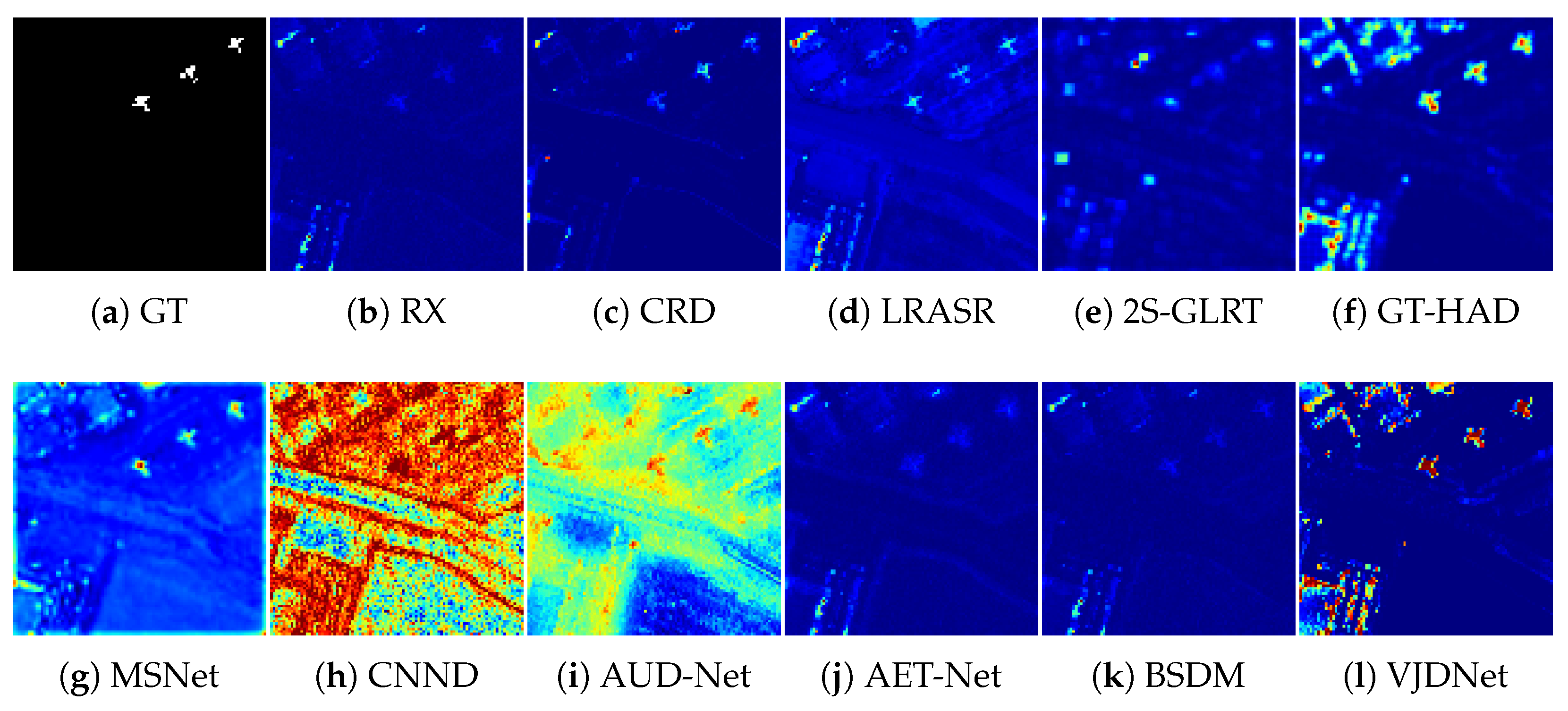
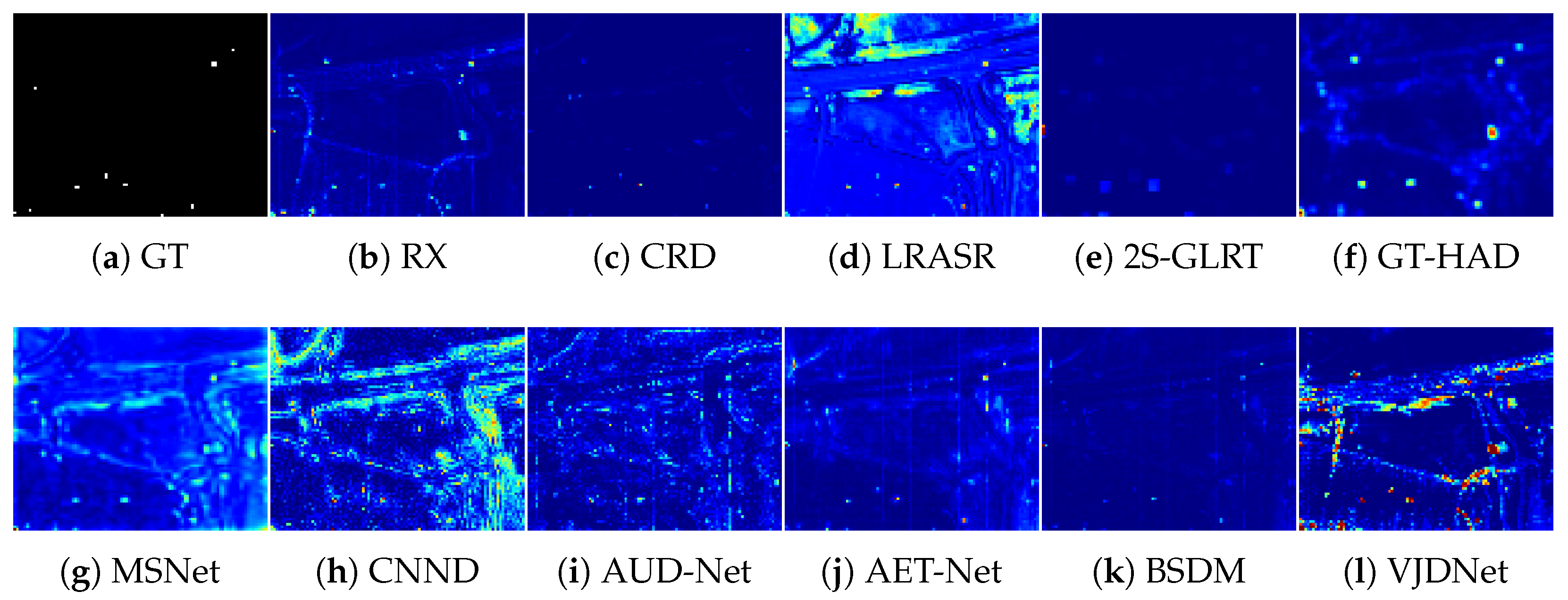
The ROC curves of different methods on various datasets are shown in Figure 4. It can be seen that, on the San Diego dataset, the VJDNet can quickly achieve a high true positive rate. On other datasets, the performance of the VJDNet can reach a similar level to other methods. We present the detection maps of cross-image detection for different methods in Figure 5, Figure 6, Figure 7 and Figure 8. It can be seen from the detection map that, compared to other methods, the VJDNet can greatly enhance the activation of anomalies.

4.5.2. Comparison on HAD-100 Dataset

To further validate the cross-image detection performance and efficiency of the VJDNet, we conducted comparative experiments on the large-scale dataset HAD-100. Similar to the experiments on individual datasets, we first trained on all images in the training set, then performed detection on the 100 test images. We compared the AUC scores and efficiency metrics of different methods, as shown in

Table 4. AUC scores, parameters, FLOPs, and inference times for different methods of cross-image detection on HAD-100 dataset.

Metric	RX	CRD	LRASR	2S-GLRT	CNND	AUD-Net	AET-Net	BSDM	VJDNet
mAUC ($P_d$, $P_f$) ↑	0.9657	0.8866	0.9290	0.9530	0.8759	0.9061	0.9726	0.9615	0.9841
mAUC ($P_d$, $\tau$) ↑	0.3494	0.3352	0.3928	0.3195	0.9075	0.0472	0.3695	0.2964	0.7085
mAUC ($P_f$, $\tau$) ↓	0.0312	0.1006	0.0606	0.0468	0.5317	0.0152	0.0522	0.0336	0.2604
Params (M) ↓	-	-	-	-	0.0377	2.3770	0.8784	0.9300	0.0168
FLOPs (G) ↓	-	-	-	-	1.3641	6543.7696	0.9331	1.4688	0.6318
Time (s) ↓	0.0865	48.2919	11.0864	2.4882	5.9839	7.5701	0.1593	1.5813	0.6943

. The FLOPs were calculated on a $64\times 64$ image, while the inference time represents the average time taken for detection on one image.

The experimental results show that the proposed VJDNet achieves the best detection performance on large-scale datasets compared to non-deep-learning methods and other cross-image methods. Although CNND has higher sensitivity to anomalies than the VJDNet, it also has the highest mAUC ($P_f$, $\tau$) score, resulting in weaker discrimination between background and anomalies. In terms of model lightweightness and detection efficiency, while the VJDNet’s inference time is slightly higher than RX and AET-Net, it achieves the lowest number of parameters and FLOPs. In general, the VJDNet exhibits remarkable generalization and stability while also featuring a lightweight network structure.

4.6. Ablation Studies

4.6.1. Effectiveness of the PDJD Module

In this section, we validate the effectiveness of the proposed PDJD module. The PDJD module combines the global reconstruction probability and the local distribution difference to jointly discriminate anomalies. Therefore, we compare the detection results of the PDJD module with methods using single discriminative information. Each method is first trained on the ABU dataset and then tested on the remaining four datasets. The detection results on the four datasets are shown in

Table 5. AUROC scores for the proposed method with different anomaly discrimination modules.

Dataset	Probability	Distribution	PDJD
San Diego	0.9340	0.9694	0.9890
Cri	0.9876	0.9815	0.9930
HYDICE	0.9648	0.9925	0.9923
WHU-Hi-River	0.9068	0.9938	0.9933
Mean	0.9483	0.9843	0.9919

. In the table, the “Probability” method uses pixel reconstruction probability as the anomaly score, which can be regarded as the basic VAE method. The “Distribution” method uses the Wasserstein distance between the latent distribution of the central pixel and the background representation as the anomaly score. To further demonstrate the performance of the VJDNet visually, we use the San Diego dataset as an example and compare the detection map after exponentiation of different methods.

The results in Table 5 show that, on the three datasets and the mean score, the proposed method using the PDJD module achieved the best performance and was only slightly inferior to the distribution-discriminant method on the WHU-Hi-River dataset. The visualization results on the San Diego dataset are shown in Figure 9. It can be observed that, compared to the method using only global reconstruction probability information, the PDJD module suppresses background activation by measuring differences with surroundings. Compared to the method using only local distribution difference information, the PDJD module significantly enhances the anomaly activation. Therefore, the proposed VJDNet can balance background suppression and anomaly enhancement and achieve good detection results on different datasets.

4.6.2. Effectiveness of the Dynamical Sample Pair Generator

To verify the effectiveness of the dynamic generation procedure, we compare four combinations of training sample pairs: static anomalies with static surroundings, static anomalies with dynamic surroundings, dynamic anomalies with static surroundings, and dynamic anomalies with dynamic surroundings. For static anomalies, we converted 20 percent of samples into anomalies as preprocessing rather than doing so every iteration. For static surroundings, we used the mean of surrounding pixels instead of the sampling process. The experimental results of the four combinations are shown in

Table 6. AUROC scores for the proposed method with different sample pair generation procedures.

Procedure		Dataset				Mean
Anomaly	Surrounding	San Diego	Cri	HYDICE	River
Static	Static	0.9777	0.9911	0.9910	0.9875	0.9868
Static	Dynamic	0.9864	0.9925	0.9930	0.9900	0.9905
Dynamic	Static	0.9820	0.9926	0.9911	0.9907	0.9891
Dynamic	Dynamic	0.9890	0.9930	0.9923	0.9933	0.9919

. The WHU-Hi-River dataset is abbreviated as River.

As seen from the results, although the static generation procedure can already perform effective detection, using the dynamic generation approach further improves the overall detection performance. Especially on San Diego and WHU-Hi-River datasets, the dynamic generation of anomalies and surroundings both significantly improve the detection results. For the HYDICE dataset, the dynamic generation of anomalies does not improve the detection performance significantly. This may be because the HYDICE dataset has relatively complex backgrounds while dynamic anomalies enhance the discriminability of the network, thus slightly increasing the probability of classifying the backgrounds as anomalies.

4.7. Parameter Analysis

In this section, we conduct experiments on the hyperparameter settings in the VJDNet, including the number of background representation samples $N_b$, the anomaly generation probability $\rho$, and the balance parameter $\lambda$ in (17). When a certain hyperparameter is evaluated, the remaining hyperparameters are consistent with the settings in Section 4.2.

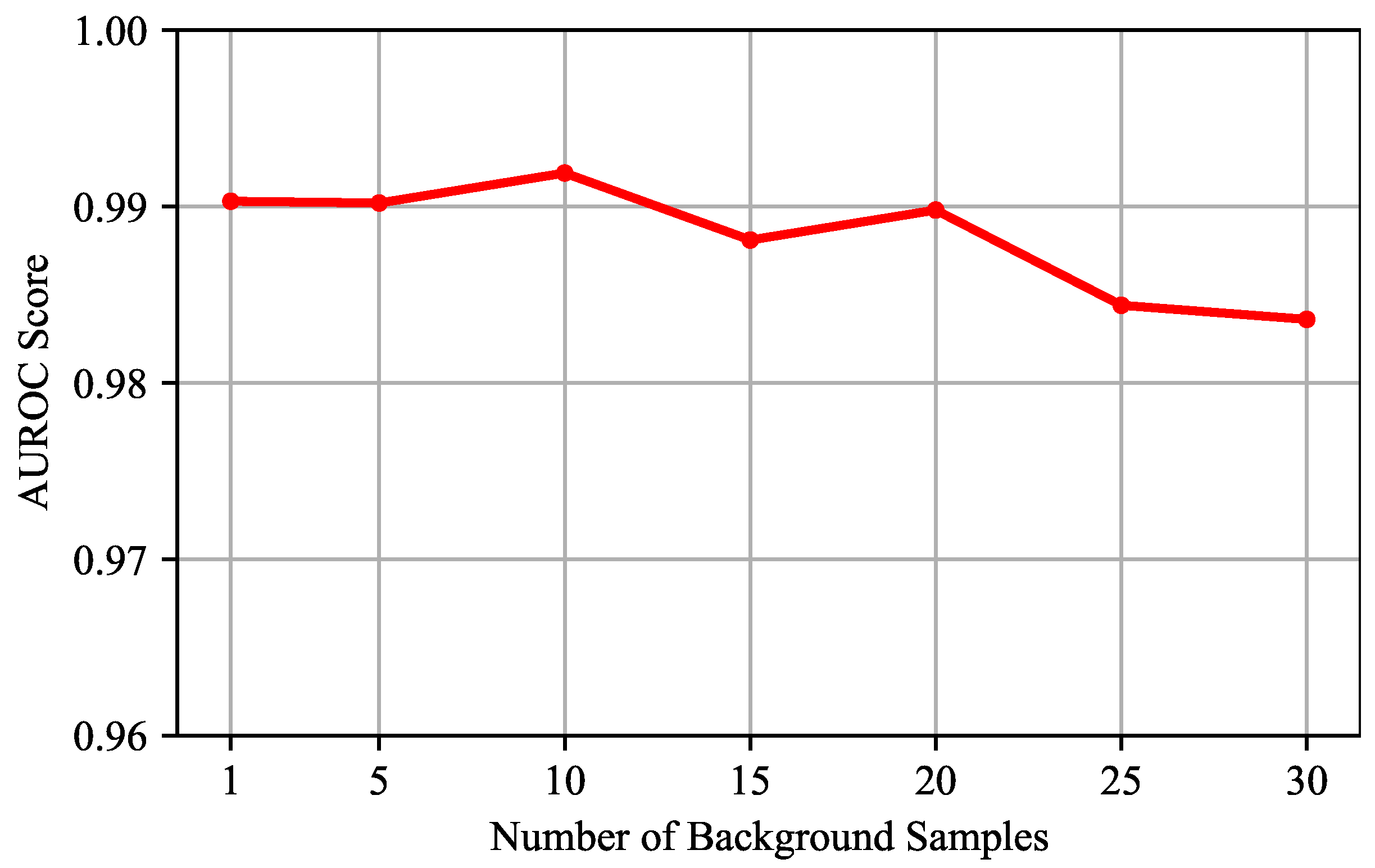
(1)

Evaluation of the Number of Background Representation Samples: We conduct experiments on different numbers of background representation samples $N_b$, which is set as [1, 5, 10, 15, 20, 25, 30]. The averages of the results on the four datasets are shown in Figure 10. The results show that, when $N_b$ is less than 20, the detection performance remains relatively stable. However, as $N_b$ becomes larger, the AUROC score gradually decreases. This may be because, with a larger $N_b$, the background representation is more likely to be close to the mean of surrounding pixels, thereby reducing diversity and weakening the generalization of the network. When $N_b$ is set to 10, the detection performance reaches the best, and the generalization and stability of the network have reached a balance.

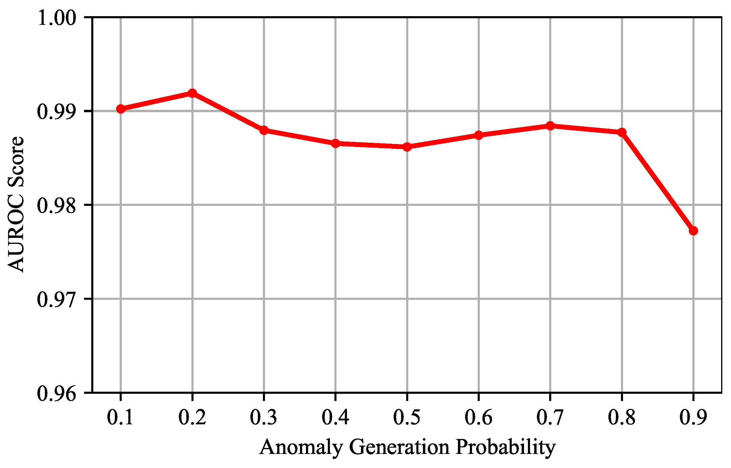
(2)

Evaluation of the Anomaly Generation Probability: We conduct experiments on different values of the anomaly generation probability $\rho$ in the range of [0.1, 0.9]. The averages of the results on the four datasets are shown in Figure 11. The results show that, when $\rho$ is 0.2, the detection performance reaches the best. When $\rho$ is set to different values, the VJDNet can achieve good results within a certain range. But, when $\rho$ reaches 0.9, the detection performance declines. It is worth noting that, when $\rho$ is large, network training may become unstable. In this case, as the number of training epochs increases, the detection performance may drop significantly. This is another reason why we have chosen a small anomaly generation probability.

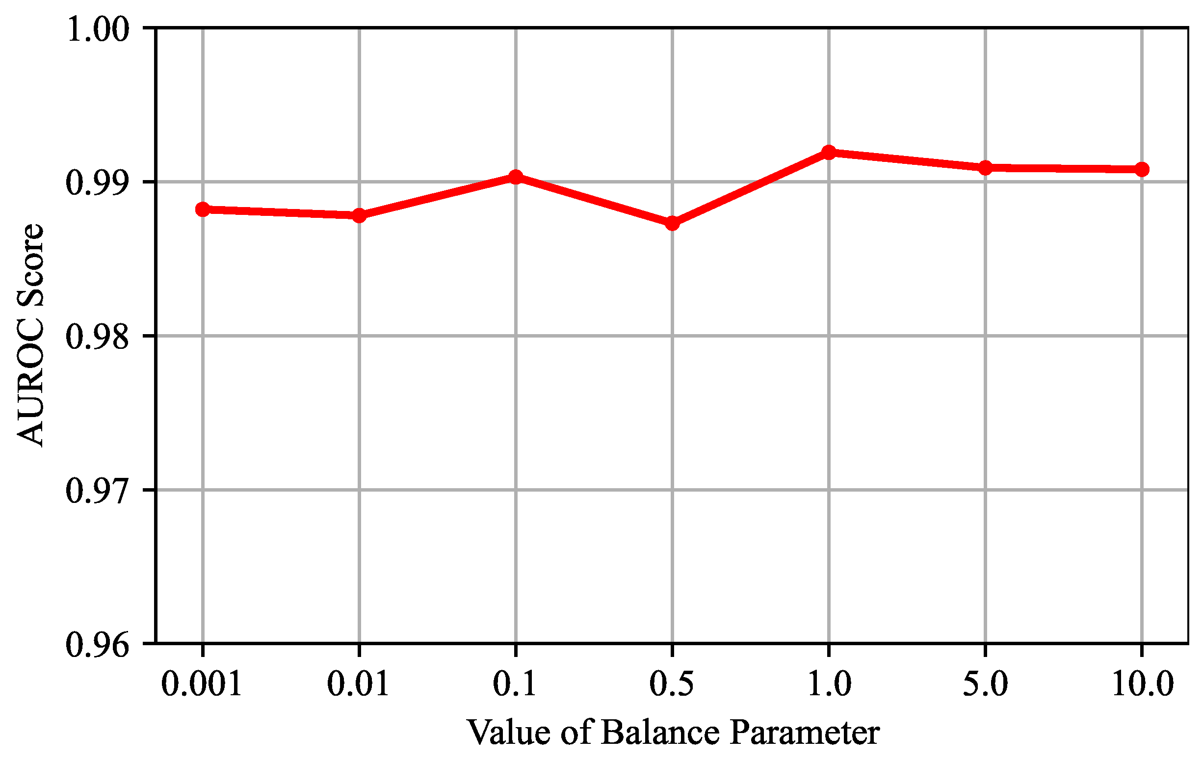
(3)

Evaluation of the Balance Parameter: We conduct experiments on different values of the balance parameter $\lambda$, which is set as [0.001, 0.01, 0.1, 0.5, 1, 5, 10]. The averages of the results on the four datasets are shown in Figure 12. The results show that the performance of the VJDNet is not sensitive to the value of $\lambda$. When $\lambda$ is set to 1, the detection performance reaches the best. Therefore, we set $\lambda$ as 1 in the experiments.

5. Conclusions

To maintain the detection performance in unknown images, the existing cross-image HAD methods often require additional supervised information or network stacking to enhance representation capabilities. However, this may impose high demands on data or hardware in practical applications. To address these shortcomings, we proposed a simple and unsupervised lightweight cross-image HAD method named VJDNet. Leveraging the reconstruction and distribution representation capabilities of the VAE, the VJDNet combines global and local information to jointly learn the pixel’s reconstruction probability and its distribution difference from surrounding pixels, thereby effectively identifying anomalies in unknown hyperspectral images. In addition, a sample pair generation module was proposed to generate anomalous pixels and surrounding background representations suitable for cross-image HAD tasks, balancing stability and generalization. We verified the single-image detection and cross-image detection performance of the VJDNet. The experimental results show that the VJDNet is able to achieve good detection performance while containing only a small number of parameters. The VJDNet also has good scalability and is expected to further improve cross-image HAD performance via more advanced networks or generating more representative anomalies and background representations.