


A Machine Learning-Based Method for Lithology Identification of Outcrops Using TLS-Derived Spectral and Geometric Features

 ,
,
Abstract
1. Introduction
- (a)
- Segmenting the outcrop point cloud into regular grid units;
- (b)
- Extracting a multidimensional feature set, including spectral features (e.g., reflectance median, mean, skewness) and geometric features (e.g., curvature, planarity, sphericity);
- (c)
- Constructing a random forest model based on the extracted features to perform lithological classification;
- (d)
- Applying post-classification corrections based on prior stratigraphic attitude information to enhance geological consistency.
- (a)
- Grid-based multi-source feature fusion method: A systematic framework was developed for feature extraction from gridded point cloud units, enabling the simultaneous acquisition of spectral reflectance statistics (e.g., median, kurtosis) and 3D geometric descriptors (e.g., surface variation, curvature, planarity). This method supports a comprehensive, multidimensional characterization of outcrop point cloud attributes, providing a strong foundation for robust lithological classification.
- (b)
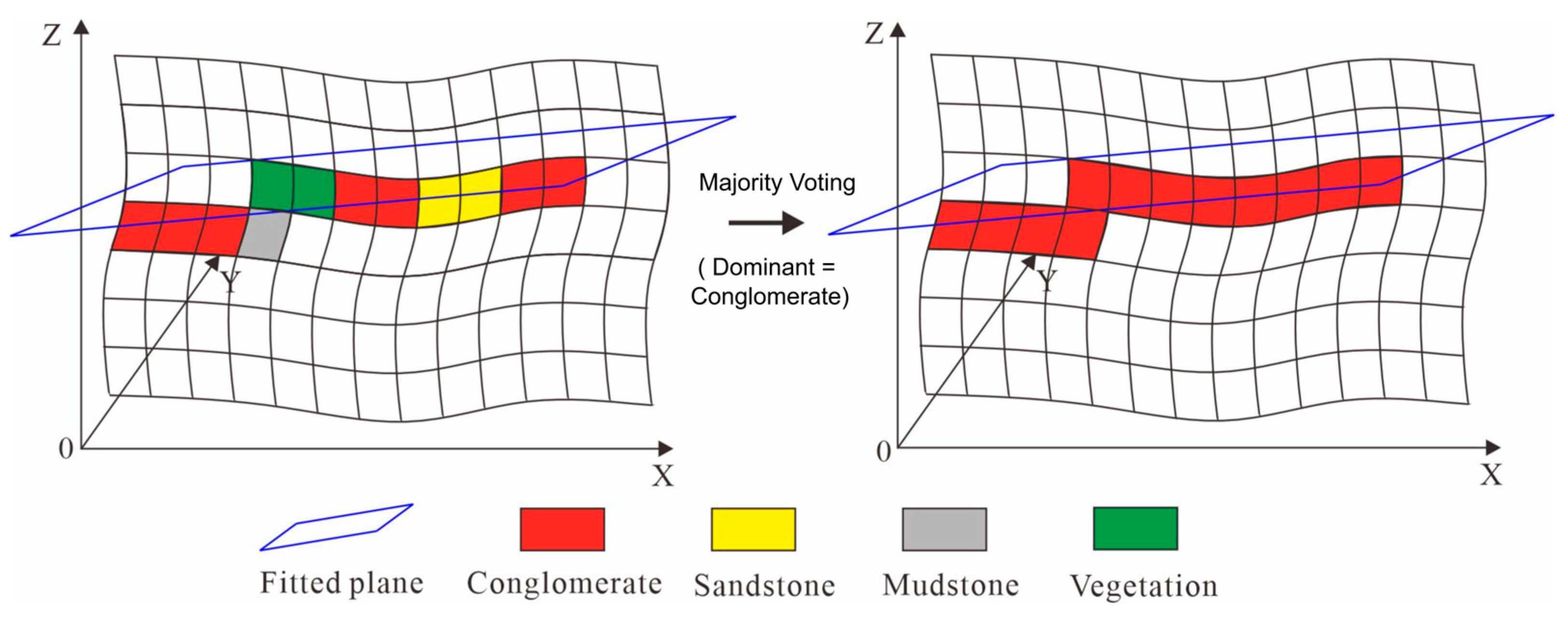
- Geology-constrained post-classification correction algorithm: A stratigraphic boundary-guided refinement strategy is proposed, incorporating geological prior knowledge—specifically, the stratigraphic principle of lateral continuity, which posits that lithologies within the same sedimentary layer tend to exhibit lateral consistency and internal homogeneity. By fitting stratigraphic surfaces and applying majority voting within each delineated layer, the method effectively reduces misclassifications caused by surface weathering or sensor-induced noise. This post-processing step significantly improves both the spatial continuity and geological plausibility of the classification results.
2. Data
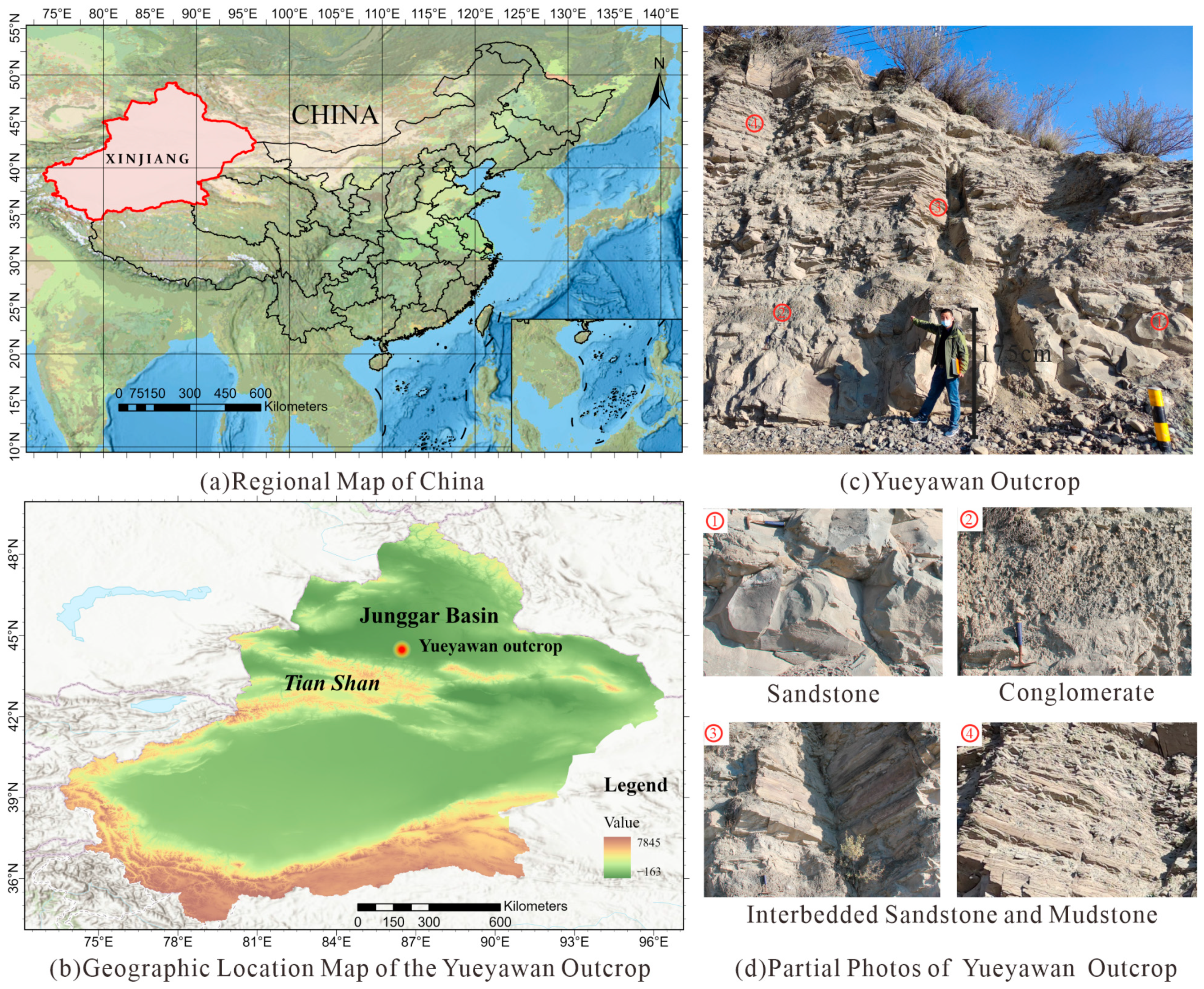
2.1. Study Area
2.2. Data Acquisition
3. Methods
3.1. Regular Grid Partitioning of Point Cloud Data
3.2. Geometric–Spectral Feature Extraction
3.2.1. Geometric Features
3.2.2. Spectral Features
3.3. Random Forest-Based Lithological Classification
3.3.1. Feature Selection
3.3.2. Double-Layer Random Forest Model Construction
3.4. Post-Processing of Stratigraphic Attitude Results
4. Results and Analysis
4.1. Evaluation Metrics
- (a)
- Overall Accuracy (OA)
- (b)
- Class-wise Evaluation Metrics
- i
- Precision measures the proportion of true positive instances among all instances predicted as positive.
- ii
- Recall measures the proportion of true positive instances among all actual positive instances.
- iii
- The F1-score is the harmonic mean of precision and recall used to address class imbalance issues.
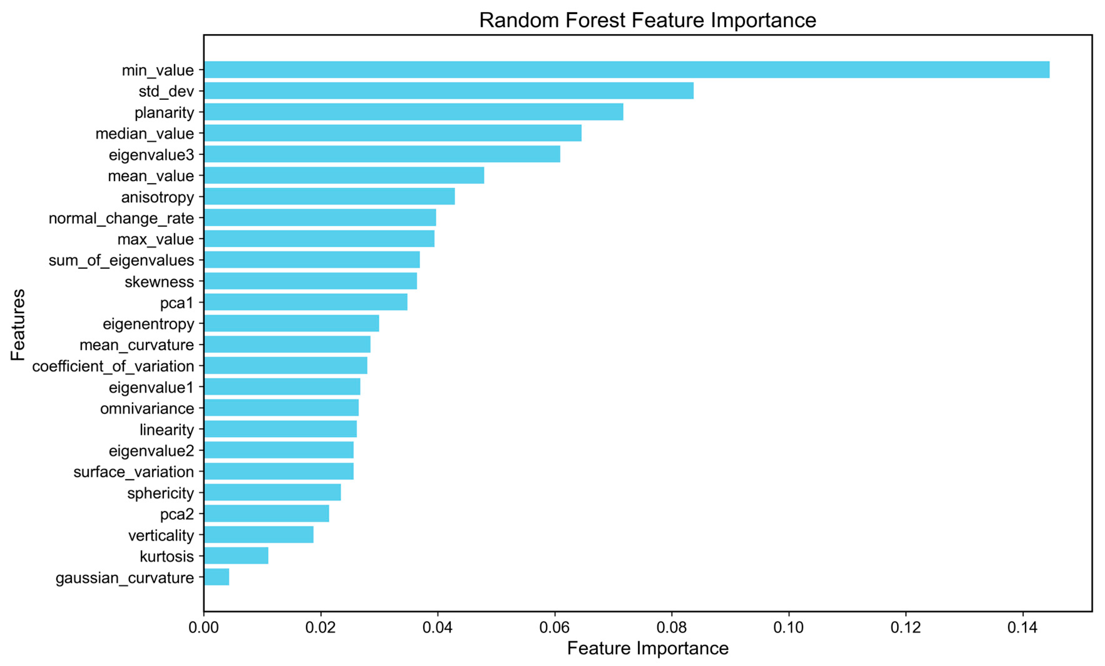
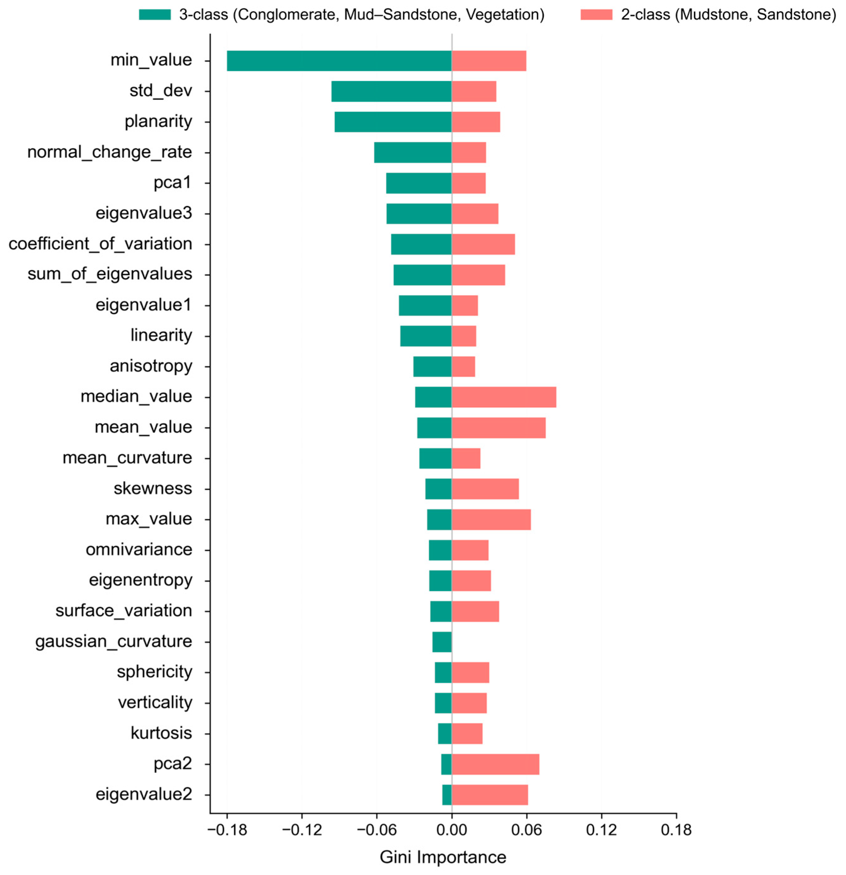
4.2. Feature Importance Analysis
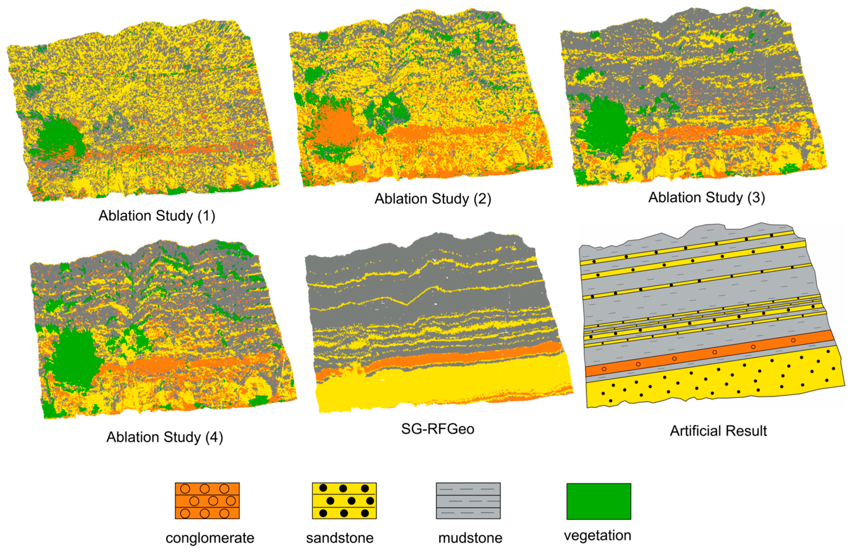
4.3. Ablation Study of Key Modules
- (1)
- Using only reflectance statistical features with a single-layer random forest classifier;
- (2)
- Using only geometric features with a single-layer random forest classifier;
- (3)
- Combining reflectance statistical and geometric features with a single-layer random forest classifier;
- (4)
- Combining reflectance statistical and geometric features with a double-layer random forest classifier without applying stratigraphic attitude constraints;
- (5)
- Combining reflectance statistical and geometric features with a double-layer random forest classifier and incorporating stratigraphic attitude constraints (i.e., SG-RFGeo).
4.4. Comparative Analysis and Performance Evaluation
5. Discussion
5.1. SG-RFGeo Effectiveness Analysis
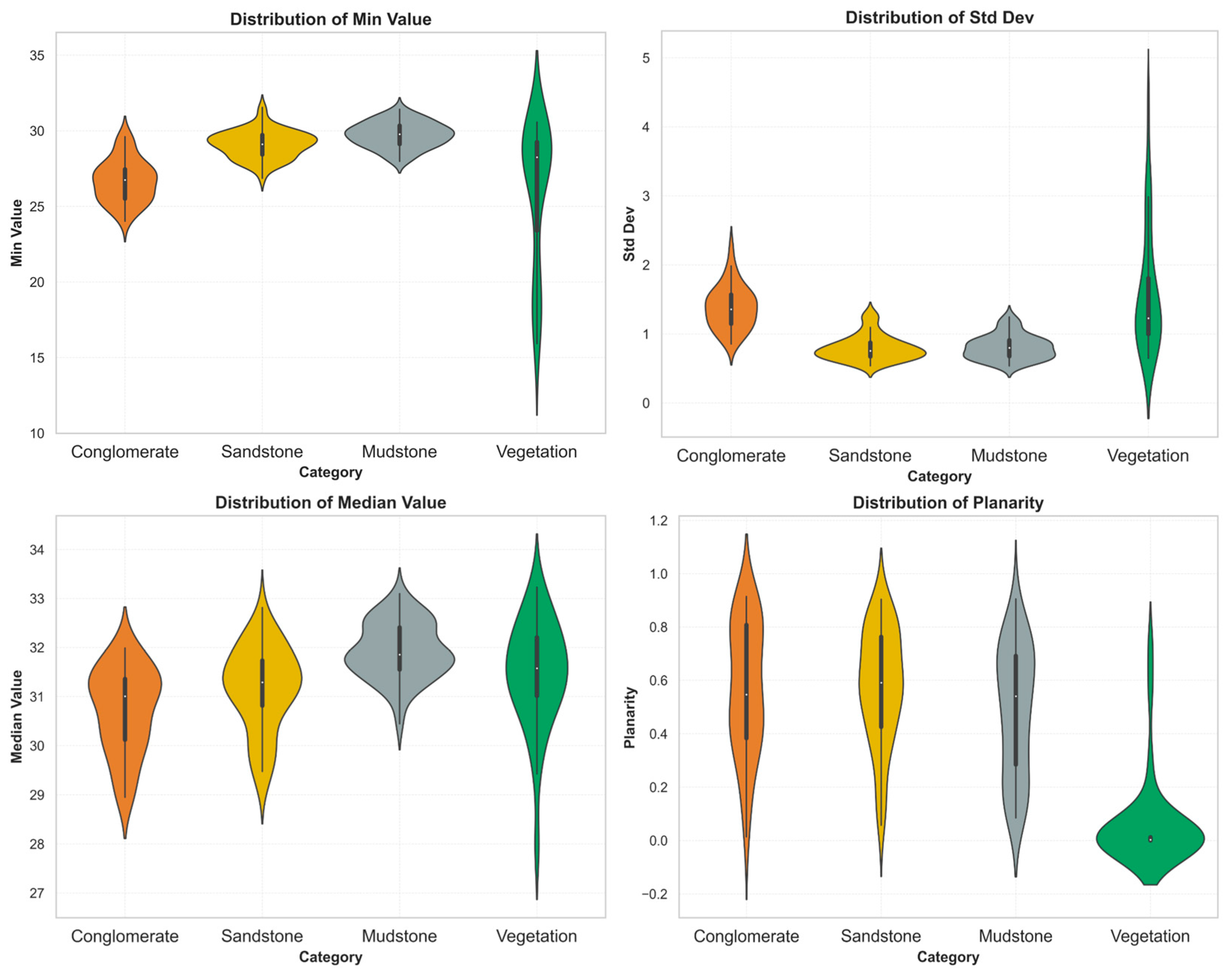
5.2. Analysis of Key Spectral–Geometric Features
5.3. Grid Resolution Effect Analysis
5.4. Case Study on Carbonate Outcrop
6. Conclusions
Supplementary Materials
Author Contributions
Funding
Data Availability Statement
Conflicts of Interest
References
- Dong, Z.; Tang, P.; Chen, G.; Yin, S. Synergistic Application of Digital Outcrop Characterization Techniques and Deep Learning Algorithms in Geological Exploration. Sci. Rep. 2024, 14, 22948. [Google Scholar] [CrossRef]
- Frykman, P. Spatial Variability in Petrophysical Properties in Upper Maastrichtian Chalk Outcrops at Stevns Klint, Denmark. Mar. Pet. Geol. 2001, 18, 1041–1062. [Google Scholar] [CrossRef]
- Nemati, M.; Pezeshk, H. Spatial Distribution of Fractures in the Asmari Formation of Iran in Subsurface Environment: Effect of Lithology and Petrophysical Properties. Nat. Resour. Res. 2005, 14, 305–316. [Google Scholar] [CrossRef]
- Abellán, A.; Calvet, J.; Vilaplana, J.M.; Blanchard, J. Detection and Spatial Prediction of Rockfalls by Means of Terrestrial Laser Scanner Monitoring. Geomorphology 2010, 119, 162–171. [Google Scholar] [CrossRef]
- Cawood, A.J.; Corradetti, A.; Granado, P.; Tavani, S. Detailed Structural Analysis of Digital Outcrops: A Learning Example from the Kermanshah-Qulqula Radiolarite Basin, Zagros Belt, Iran. J. Struct. Geol. 2022, 154, 104489. [Google Scholar] [CrossRef]
- Villarreal, C.A.; Garzón, C.G.; Mora, J.P.; Rojas, J.D.; Ríos, C.A. Workflow for Capturing Information and Characterizing Difficult-to-Access Geological Outcrops Using Unmanned Aerial Vehicle-Based Digital Photogrammetric Data. J. Ind. Inf. Integr. 2022, 26, 100292. [Google Scholar] [CrossRef]
- Yin, S.L.; Chen, G.Y.; Liu, Z.L.; Feng, W.; Liu, Y. 3D Digital Outcrop Characterization Technology based on Unmanned Aerial Vehicle Oblique Photography. Acta Sedimentol. Sin. 2018, 36, 72–80. [Google Scholar]
- Chang, L.; Han, L.; Chen, Z.Q.; Sheng, H.; Liu, S.W. Lithology classification of large slope geological outcrop based on UAV multi spectral remote sensing. Bull. Surv. Mapp. 2023, 42–47. [Google Scholar] [CrossRef]
- Bishop, C.; Rivard, B.; De Souza Filho, C.; Van Der Meer, F. Geological Remote Sensing. Int. J. Appl. Earth Obs. Geoinf. 2018, 64, 267–274. [Google Scholar] [CrossRef]
- Bellian, J.A.; Kerans, C.; Jennette, D.C. Digital Outcrop Models: Applications of Terrestrial Scanning Lidar Technology in Stratigraphic Modeling. J. Sediment. Res. 2005, 75, 166–176. [Google Scholar] [CrossRef]
- Amrullah, C.; Suwardhi, D.; Meilano, I. Product Accuracy Effect of Oblique and Vertical Non-Metric Digital Camera Utilization in Uav-Photogrammetry to Determine Fault Plane. ISPRS Ann. Photogramm. Remote Sens. Spat. Inf. Sci. 2016, 3, 41–48. [Google Scholar] [CrossRef]
- Rashidi, M.; Mohammadi, M.; Sadeghlou Kivi, S.; Abdolvand, M.M.; Truong-Hong, L.; Samali, B. A Decade of Modern Bridge Monitoring Using Terrestrial Laser Scanning: Review and Future Directions. Remote Sens. 2020, 12, 3796. [Google Scholar] [CrossRef]
- Buckley, S.J.; Enge, H.D.; Carlsson, C.; Howell, J.A. Terrestrial Laser Scanning for Use in Virtual Outcrop Geology. Photogramm. Rec. 2010, 25, 225–239. [Google Scholar] [CrossRef]
- Tomás, R.; Li, Z. Earth Observations for Geohazards: Present and Future Challenges. Remote Sens. 2017, 9, 194. [Google Scholar] [CrossRef]
- Zhang, D.; Wu, Z.; Shi, D.; Li, J.; Lu, Y. Integration of Terrestrial Laser Scanner (TLS) and Ground Penetrating Radar (GPR) to Characterize the Three-Dimensional (3D) Geometry of the Maoyaba Segment of the Litang Fault, Southeastern Tibetan Plateau. Remote Sens. 2022, 14, 6394. [Google Scholar] [CrossRef]
- Qiu, J.L.; Xia, Q.L.; Yao, L.Q.; Yuan, Z.X.; Shi, C. Mine Geological Modeling and Application Based on the Three-Dimensional Laser Scanner Technology. Earth Sci./Diqiu Kexue 2012, 37, 1209–1216. [Google Scholar]
- Abellán, A.; Oppikofer, T.; Jaboyedoff, M.; Rosser, N.J.; Lim, M.; Lato, M.J. Terrestrial Laser Scanning of Rock Slope Instabilities. Earth Surf. Process. Landf. 2014, 39, 80–97. [Google Scholar] [CrossRef]
- Ge, Y.F.; Xia, D.; Tang, H.M.; Zhao, B.B.; Wang, L.Q.; Chen, Y. Intelligent identification and extraction of geometric properties of rock discontinuities based on terrestrial laser scanning. Chin. J. Rock Mech. Eng. 2017, 36, 3050–3061. [Google Scholar] [CrossRef]
- Van Genderen, J.L. Airborne and Terrestrial Laser Scanning. Int. J. Digit. Earth 2011, 4, 183–184. [Google Scholar] [CrossRef]
- Telling, J.; Lyda, A.; Hartzell, P.; Glennie, C. Review of Earth Science Research Using Terrestrial Laser Scanning. Earth-Sci. Rev. 2017, 169, 35–68. [Google Scholar] [CrossRef]
- Burton, D.; Dunlap, D.B.; Wood, L.J.; Flaig, P.P. Lidar Intensity as a Remote Sensor of Rock Properties. J. Sediment. Res. 2011, 81, 339–347. [Google Scholar] [CrossRef]
- Hartzell, P.; Glennie, C.; Biber, K.; Khan, S. Application of Multispectral LiDAR to Automated Virtual Outcrop Geology. ISPRS J. Photogramm. Remote Sens. 2014, 88, 147–155. [Google Scholar] [CrossRef]
- Humair, F.; Abellan, A.; Carrea, D.; Matasci, B.; Epard, J.-L.; Jaboyedoff, M. Geological Layers Detection and Characterisation Using High Resolution 3D Point Clouds: Example of a Box-Fold in the Swiss Jura Mountains. Eur. J. Remote Sens. 2015, 48, 541–568. [Google Scholar] [CrossRef]
- Živec, T.; Anžur, A.; Verbovšek, T. Determination of Rock Type and Moisture Content in Flysch Using TLS Intensity in the Elerji Quarry (South-West Slovenia). Bull. Eng. Geol. Environ. 2019, 78, 1631–1643. [Google Scholar] [CrossRef]
- Riquelme, A.; Tomás, R.; Cano, M.; Pastor, J.L.; Abellán, A. Automatic Mapping of Discontinuity Persistence on Rock Masses Using 3D Point Clouds. Rock Mech. Rock Eng. 2018, 51, 3005–3028. [Google Scholar] [CrossRef]
- Brodu, N.; Lague, D. 3D Terrestrial Lidar Data Classification of Complex Natural Scenes Using a Multi-Scale Dimensionality Criterion: Applications in Geomorphology. ISPRS J. Photogramm. Remote Sens. 2012, 68, 121–134. [Google Scholar] [CrossRef]
- Walton, G.; Mills, G.; Fotopoulos, G.; Radovanovic, R.; Stancliffe, R.P.W. An Approach for Automated Lithological Classification of Point Clouds. Geosphere 2016, 12, 1833–1841. [Google Scholar] [CrossRef]
- Chen, J.; Wang, B.; Wang, F.; Hou, M.; Hu, Z. Identification of Outcropping Strata from UAV Oblique Photogrammetric Data Using a Spatial Case-Based Reasoning Model. Int. J. Appl. Earth Obs. Geoinf. 2021, 103, 102450. [Google Scholar] [CrossRef]
- Penasa, L.; Franceschi, M.; Preto, N.; Teza, G.; Polito, V. Integration of Intensity Textures and Local Geometry Descriptors from Terrestrial Laser Scanning to Map Chert in Outcrops. ISPRS J. Photogramm. Remote Sens. 2014, 93, 88–97. [Google Scholar] [CrossRef]
- Weidner, L.; Walton, G.; Kromer, R. Classification Methods for Point Clouds in Rock Slope Monitoring: A Novel Machine Learning Approach and Comparative Analysis. Eng. Geol. 2019, 263, 105326. [Google Scholar] [CrossRef]
- Carrea, D.; Abellan, A.; Humair, F.; Matasci, B.; Derron, M.-H.; Jaboyedoff, M. Correction of Terrestrial LiDAR Intensity Channel Using Oren–Nayar Reflectance Model: An Application to Lithological Differentiation. ISPRS J. Photogramm. Remote Sens. 2016, 113, 17–29. [Google Scholar] [CrossRef]
- Ercoli, L.; Megna, B.; Nocilla, A.; Zimbardo, M. Measure of a Limestone Weathering Degree Using Laser Scanner. Int. J. Archit. Herit. 2013, 7, 591–607. [Google Scholar] [CrossRef]
- Buckley, S.J.; Kurz, T.H.; Howell, J.A.; Schneider, D. Terrestrial Lidar and Hyperspectral Data Fusion Products for Geological Outcrop Analysis. Comput. Geosci. 2013, 54, 249–258. [Google Scholar] [CrossRef]
- Hallam, A. Seismic Stratigraphy and Global Changes. Nature 1978, 272, 400. [Google Scholar] [CrossRef]
- Mousavi, S.H.R.; Hosseini-Nasab, S.M. A Novel Approach to Classify Lithology of Reservoir Formations Using GrowNet and Deep-Insight with Physic-based Feature Augmentation. Energy Sci. Eng. 2024, 12, 4453–4477. [Google Scholar] [CrossRef]
- Wang, J.; Pang, Y.; Cao, Y.; Peng, J.; Liu, K.; Liu, H. Sedimentary Environment Constraints on the Diagenetic Evolution of Clastic Reservoirs: Examples from the Eocene “Red-Bed” and “Gray-Bed” in the Dongying Depression, China. Mar. Pet. Geol. 2021, 131, 105153. [Google Scholar] [CrossRef]
- Hackel, T.; Wegner, J.D.; Schindler, K. Contour Detection in Unstructured 3D Point Clouds. In Proceedings of the 2016 IEEE Conference on Computer Vision and Pattern Recognition (CVPR), Las Vegas, NV, USA, 27–30 June 2016; IEEE: New York, NJ, USA, 2016; pp. 1610–1618. [Google Scholar]
- Weinmann, M.; Jutzi, B.; Hinz, S.; Mallet, C. Semantic Point Cloud Interpretation Based on Optimal Neighborhoods, Relevant Features and Efficient Classifiers. ISPRS J. Photogramm. Remote Sens. 2015, 105, 286–304. [Google Scholar] [CrossRef]
- Freski, Y.R.; Hecker, C.; Meijde, M.V.D.; Setianto, A. Remote Detection of Geothermal Alteration Using Airborne Light Detection and Ranging Return Intensity. Remote Sens. 2024, 16, 1646. [Google Scholar] [CrossRef]
- Franceschi, M.; Teza, G.; Preto, N.; Pesci, A.; Galgaro, A.; Girardi, S. Discrimination between Marls and Limestones Using Intensity Data from Terrestrial Laser Scanner. ISPRS J. Photogramm. Remote Sens. 2009, 64, 522–528. [Google Scholar] [CrossRef]
- Haest, M.; Cudahy, T.; Laukamp, C.; Gregory, S. Quantitative Mineralogy from Infrared Spectroscopic Data. I. Validation of Mineral Abundance and Composition Scripts at the Rocklea Channel Iron Deposit in Western Australia. Econ. Geol. 2012, 107, 209–228. [Google Scholar] [CrossRef]


| Model | Pulse Frequency (kHz) | Data Acquisition Rate (pts/s) | Scanning Speed (lines/s) | Field of View (°) | Range Accuracy (mm @ m) | Angular Resolution (°) |
|---|---|---|---|---|---|---|
| RIEGL VZ400 | 1200 | 500,000 | <100 | 360 × 100 | ±5 mm @ 50 m | <0.001 |
| Class | Samples |
|---|---|
| Vegetation | 3369 |
| Conglomerate | 3800 |
| Sandstone | 5500 |
| Mudstone | 4899 |
| Feature Parameters | Formulas | Visualizations | Feature Parameters | Formulas | Visualizations | ||
|---|---|---|---|---|---|---|---|
| 1 | Mean curvature |  | 2 | Gaussian curvature |  | ||
| 3 | PCA (PCA1, PCA2) |  | 4 | Sum of eigenvalues |  | ||
| 5 | Anisotropy |  | 6 | Planarity |  | ||
| 7 | Linearity |  | 8 | Sphericity |  | ||
| Feature Parameters | Formulas | Visualizations | |||||
| 9 | Verticality |  | |||||
| 10 | Normal change rate |  | |||||
| 11 | Eigenvalue (λ1, λ2, λ3) |  | |||||
| 12 | Omnivariance |  | |||||
| 13 | Eigenentropy |  | |||||
| 14 | Surface variation |  | |||||
| Feature Parameters | Formulas | Visualizations | Feature Parameters | Formulas | Visualizations | ||
|---|---|---|---|---|---|---|---|
| 1 | Max |  | 2 | Min |  | ||
| 3 | Mean |  | 4 | Coefficient of Variation |  | ||
| Feature Parameters | Formulas | Visualizations | |||||
| 5 | Median |  | |||||
| 6 | Standard Deviation |  | |||||
| 7 | Skewness |  | |||||
| 8 | Kurtosis |  | |||||
| Stage | Parameter | Value | Purpose |
|---|---|---|---|
| Coarse classification (shallow layer) | n_estimators | 100 | Balance accuracy and computation cost |
| max_depth | 20 | Prevent overfitting while capturing key features | |
| min_samples_leaf | 15 | Ensure statistical robustness at each leaf node | |
| Fine classification (deep layer) | n_estimators | 200 | Improve sensitivity to subtle class differences |
| max_depth | 30 | Enhance feature representation capability | |
| min_samples_leaf | 15 | Maintain consistency of decision rules |
| Predicted Positive | Predicted Negative | |
|---|---|---|
| Actual Positive | TP | FN |
| Actual Negative | FP | TN |
| OA | Macro Precision | Macro Recall | Macro F1-Score | |
|---|---|---|---|---|
| I | 0.632 | 0.655 | 0.648 | 0.650 |
| II | 0.655 | 0.662 | 0.662 | 0.658 |
| III | 0.805 | 0.823 | 0.819 | 0.821 |
| IV | 0.868 | 0.872 | 0.869 | 0.869 |
| V | 0.930 | 0.916 | 0.931 | 0.923 |
| OA | Macro Precision | Macro Recall | Macro F1-Score | |
|---|---|---|---|---|
| K-means | 0.449 | 0.443 | 0.440 | 0.439 |
| PointNet | 0.753 | 0.752 | 0.768 | 0.752 |
| SVM | 0.592 | 0.601 | 0.614 | 0.606 |
| XGBoost | 0.678 | 0.732 | 0.686 | 0.704 |
| SG-RFGeo | 0.930 | 0.916 | 0.931 | 0.923 |
| OA | Macro Precision | Macro Recall | Macro F1-Score | |
|---|---|---|---|---|
| 5 mm | 0.578 | 0.592 | 0.601 | 0.590 |
| 10 mm | 0.930 | 0.916 | 0.931 | 0.923 |
| 20 mm | 0.507 | 0.351 | 0.551 | 0.426 |
| Precision | Recall | F1-Score | OA | |
|---|---|---|---|---|
| algal dolomite | 0.735 | 0.818 | 0.774 | 0.861 |
| silty crystalline dolomite | 0.948 | 0.853 | 0.898 | |
| argillaceous shale | 0.767 | 0.943 | 0.846 |
Disclaimer/Publisher’s Note: The statements, opinions and data contained in all publications are solely those of the individual author(s) and contributor(s) and not of MDPI and/or the editor(s). MDPI and/or the editor(s) disclaim responsibility for any injury to people or property resulting from any ideas, methods, instructions or products referred to in the content. |
© 2025 by the authors. Licensee MDPI, Basel, Switzerland. This article is an open access article distributed under the terms and conditions of the Creative Commons Attribution (CC BY) license (https://creativecommons.org/licenses/by/4.0/).
Share and Cite
Shao, Y.; Li, P.; Jing, R.; Shao, Y.; Liu, L.; Zhao, K.; Gan, B.; Duan, X.; Li, L. A Machine Learning-Based Method for Lithology Identification of Outcrops Using TLS-Derived Spectral and Geometric Features. Remote Sens. 2025, 17, 2434. https://doi.org/10.3390/rs17142434
Shao Y, Li P, Jing R, Shao Y, Liu L, Zhao K, Gan B, Duan X, Li L. A Machine Learning-Based Method for Lithology Identification of Outcrops Using TLS-Derived Spectral and Geometric Features. Remote Sensing. 2025; 17(14):2434. https://doi.org/10.3390/rs17142434
Chicago/Turabian StyleShao, Yanlin, Peijin Li, Ran Jing, Yaxiong Shao, Lang Liu, Kunpeng Zhao, Binqing Gan, Xiaolei Duan, and Longfan Li. 2025. "A Machine Learning-Based Method for Lithology Identification of Outcrops Using TLS-Derived Spectral and Geometric Features" Remote Sensing 17, no. 14: 2434. https://doi.org/10.3390/rs17142434
APA StyleShao, Y., Li, P., Jing, R., Shao, Y., Liu, L., Zhao, K., Gan, B., Duan, X., & Li, L. (2025). A Machine Learning-Based Method for Lithology Identification of Outcrops Using TLS-Derived Spectral and Geometric Features. Remote Sensing, 17(14), 2434. https://doi.org/10.3390/rs17142434