1. Introduction
Land surface temperature (LST) is one of the key factors in the physical process of land surface at regional and global scales and has been identified as an important environmental climate variable by the global climate observing system (GCOS) [
1]. At present, LST is widely used in surface energy balance [
2,
3], global climate change [
4], urban heat island monitor [
5,
6], etc.
The thermal infrared satellite remote sensing method can reflect the continuous spatial distribution and dynamic change information of LST on a large scale and has gradually become a major way to get thermal infrared data [
7,
8]. However, due to the limitation of remote sensing satellite payload and the bottleneck of sensor manufacturing technology, there are limitations in spatial and temporal resolution for current thermal infrared satellite data [
9]. At present, the thermal infrared data obtained through satellites are mainly divided into two categories: one is the high spatial and low temporal resolution data, which is rich in details and suitable for small-scale thermal environment research. However, the revisit cycle is long, and it is vulnerable to the impact of observation conditions (such as cloud cover), which makes it difficult to achieve dynamic monitoring [
10,
11,
12,
13]. The other is thermal infrared data with high temporal and low spatial resolution. These data have a short return period and are suitable for dynamic monitoring of the thermal environment, but the spatial details are insufficient to accurately depict the variation of regional surface thermal environment [
14,
15,
16,
17,
18,
19,
20]. From the above analysis, a single spaceborne thermal infrared sensor cannot have both high temporal and spatial resolution and cannot meet the need of a study on a dynamic thermal environment in large-scale areas, which greatly limits the application of LST data [
21]. The LST downscaling algorithm can solve the problem of unbalanced spatial and temporal resolution of satellite-acquired LST data and obtain LST data with both high spatial and temporal resolution.
LST downscaling method improves spatial resolution by enhancing the spatial details of LST data. These algorithms can be divided into image fusion and scale factor algorithms [
22].
Image fusion algorithms can be roughly divided into two categories: transformation models and reconstruction models [
23]. The fusion algorithm based on the transformation model mainly utilizes the transformation model to perform a series of processing such as filtering and decomposition on the data and further relies on the inverse transformation model to reconstruct the processed data, ultimately obtaining the high-resolution data of the target. The more typical fusion algorithms based on transformation models include principal component analysis transformation [
24], saturation luminance transformation [
25], and wavelet transformation [
26], among others. The fusion algorithm based on the transformation model is less used because it cannot capture the changes in surface reflectance caused by different ground objects. The basis of the fusion algorithm based on the reconstruction model is the decomposition of pixels. Firstly, by decomposing multiple low spatial resolution data at different time phases, the variation relationship of the low spatial resolution data obtained at different times is obtained. Then, corresponding to the high spatial resolution data, the variation model between the high and low spatial resolution data is obtained. The high spatial resolution data at the final required moment can be obtained through interpolation algorithms. With the in-depth research, the fusion model based on reconstruction has been more widely applied in recent years. In recent years, many spatio-temporal fusion methods have been researched, such as the spatio-temporal adaptive reflection fusion model (STARFM) [
27], spatio-temporal data fusion approach (STDFA) model [
28], flexible spatial-temporal data fusion (FSDAF) [
29], and other models. These models have achieved fine fusion results in the visible and near-infrared bands. However, due to the essential differences between thermal infrared and visible near-infrared data, the fusion method needs to be combined with the scale factor method when used for the fusion of thermal infrared data.
The scale factor algorithm introduces spatial and spectral information of visible and near-infrared multispectral data into the process of the LST downscaling model, which is favored in thermal infrared image sharpening. Kustas et al. proposed a disaggregation procedure for the radiometric surface temperature (DisTrad) algorithm, which established the relationship between the LST and the normalized vegetation index (NDVI) and realized sub-pixel decomposition in the thermal infrared band [
30]. Agam et al. improved the DisTrad algorithm and proposed the thermal sharpening (TsHARP) algorithm. This algorithm has achieved better downscaling results than the DisTrad algorithm and obtained LST data with fine spatial and temporal resolution [
31,
32]. Since then, many researchers have improved the DisTrad and TsHARP algorithms by selecting different regression factors or changing the regression model [
33,
34,
35,
36]. The development process of the LST downscaling algorithm began with considering LST and single auxiliary parameter regression modeling in areas with relatively uniform ground features such as plains initially. With the expansion of ground feature types in the study area, in order to improve the accuracy of the LST downscaling model, more auxiliary parameters were selected for modeling. With the continuous optimization of the regression relationship model, the accuracy of the scaling algorithm is getting higher and higher. However, the above model does not consider the geospatial correlation between LST and auxiliary parameters and establishes the regression relationship between LST and auxiliary parameters in the entire study area. The research of the above models is all based on the assumption of spatial stationarity during the modeling process, that is, the relationship between LST and auxiliary parameters is consistent throughout the entire study area. However, due to the spatial heterogeneity of the study area, LST and each auxiliary parameter, as spatial variables, have a non-stationary relationship between them, causing the regression relationship among the parameters to change with the variation of spatial position. Therefore, the assumption of stationarity between LST and auxiliary parameters is not reasonable enough. With more in-depth exploration, researchers began to consider the non-stationary relationship between LST and auxiliary parameters in the modeling process.
The above methods are all based on the assumption of scale invariance, that is, the regression relationship between LST and auxiliary parameters will not change with the resolution changing. However, scale effect exists in heterogenous regions, so the assumption of scale invariance is not reasonable. In recent years, with the progress of LST scale reduction algorithms and the research on scale effects, some scholars have begun to discuss the issue of scale effects in the LST scale reduction process. In 2022, Wang et al. considered the scale effect in the LST downscaling process and proposed an LST downscaling algorithm based on Taylor expansion. This algorithm has achieved better results in urban and plain areas [
37]. However, the downscaling results in rugged terrain areas was worse than those in urban and plain areas. In many studies, the elevation was selected as the auxiliary factor in the downscaling process to eliminate the impact of terrain on LST [
38,
39], while the results of downscaling are not satisfactory.
There are many factors affecting the LST in rugged terrain areas. The thermal environment in rugged terrain is not only determined by land cover, as in plain areas, but also by the elevation and the re-distributed solar radiation because of the topographic effect [
40]. Ignoring the topographic effect will greatly hinder the study of LST in rugged areas. When the solar radiation reaches the ground, part of it is reflected and part of it is absorbed by the ground, which makes the ground heat up. Thus, the unevenly distributed solar radiation in rugged terrains becomes a major driving factor to form the spatial pattern of LST distribution. In the process of LST downscaling in rugged terrain areas, only adding elevation as an auxiliary factor cannot fully reflect the change of rugged terrain LST. The energy of the solar incident radiation is concentrated in the shortwave band, which plays an important role in the surface energy balance and is a significant factor affecting the LST. Therefore, this study will take the downward surface shortwave radiation (DSSR) as one of the auxiliary parameters for LST downscaling and use the Landsat 8 LST as reference data to verify the LST downscaling results.
2. Study Area and Datasets
Study Area
This study selects two rugged terrain regions as the study area to test the proposed algorithm in this study.
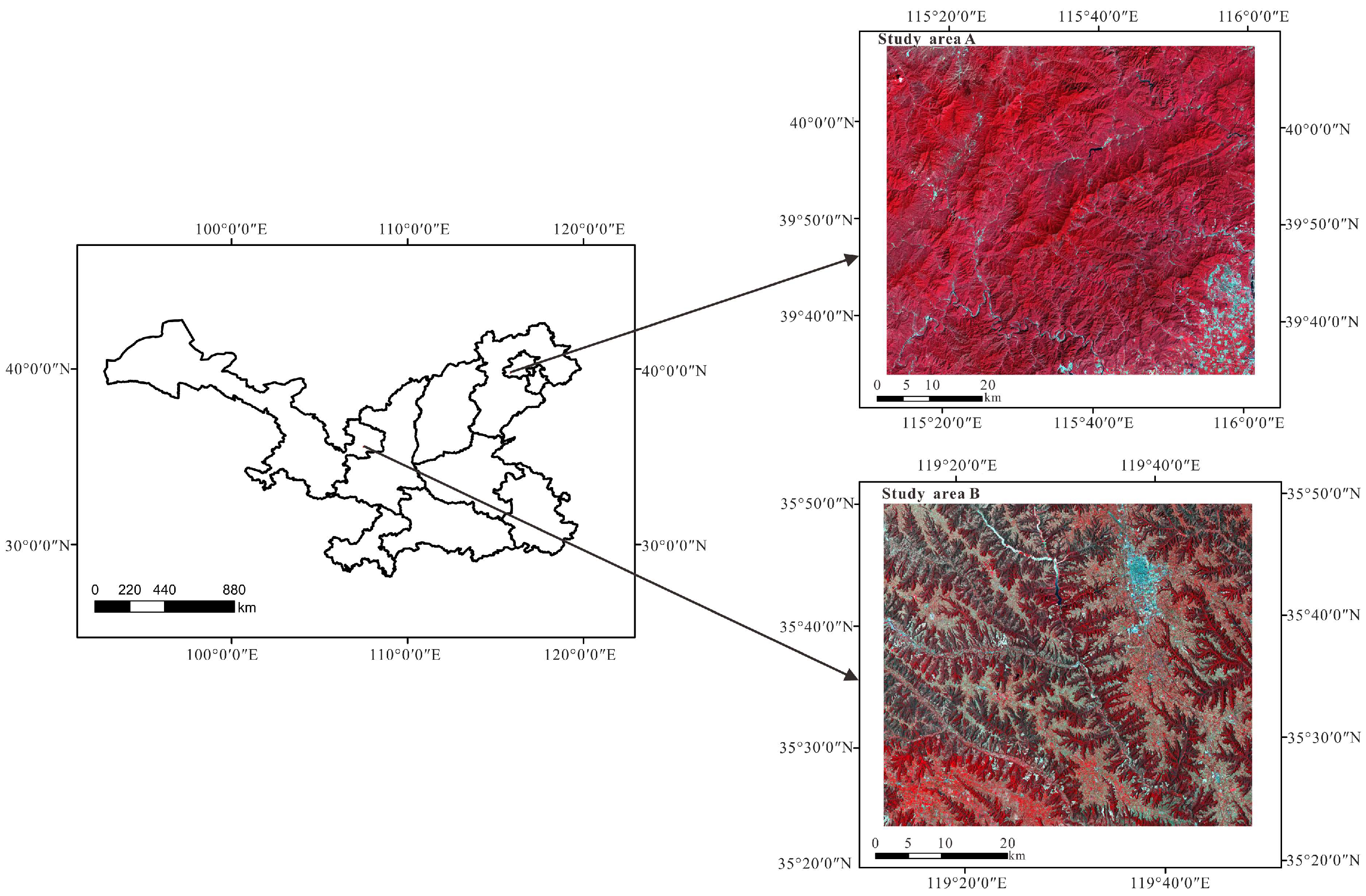
Figure 1 shows the geographical location of the study area and the false color image generated from Landsat 8 data.
Study area a is in the west suburb of Beijing, with the latitude about 115°20′0″~116°20′0″E and longitude about 39°40′0″~40°00′0″N. It located in the transition zone from the North China Plain to the Mongolian Plateau, with an average altitude of about 1500 m. The total coverage is 64,000 km2. This area belongs to the continental monsoon climate of mid latitude, with an annual average temperature of about 10 °C and an annual average precipitation of 600 mm. The forest coverage rate in the study area is 40–60%, and the land covers are mainly shrubbery and a mixed forest of miscellaneous trees.
Study area b is located in Gansu Province, with the latitude about 119°20′0″~120°00′0″E and longitude about 35°20′0″~35°50′0″N. It is on the edge of the Loess Plateau in northern China, with an altitude of 890–2857 m. The total coverage is 9000 km2. It belongs to the cold temperate semi-humid area, with an annual average temperature of about 9 °C. The terrain of the selected study area is complex and diverse due to the influence of terrain and altitude.
In this study, the LST data with 1000 m spatial resolution are downscaled to 100 m. The MODIS LST data products (MOD11_L2) are selected as low resolution LST data, and Landsat 8 data are selected to calculate the auxiliary parameters used in the LST downscaling process. The Downward shortwave solar radiation (DSSR) data required for this study is obtained through Landsat 8 and DEM data. In addition, this study uses the LST retrieved by Landsat 8 as the reference data to verify the downscale results. Therefore, this study needs MODIS LST, Landsat 8 data both in NVIR and thermal infrared bands, and DEM data.
Table 1 shows the data used in this study and the time of data acquisition. In this study, the LST data represent daytime temperature.
The MODIS data used in this study are the MODIS LST product (MOD11_L2), which is a MODIS secondary product with a spatial resolution of 1000 m, including LST data, quality control, 31 and 32 band emissivity, observation zenith angle, observation time, and other data information.
MOD11_L2 data is the data product after geometric correction and radiometric correction, and the data format adopted is the Hierarchical Data Format (HDF). The LST is inversed by the generalized split window (GSW) algorithm, and its accuracy can be within 2K in most areas [
41,
42]. The data used in this study is provided by NASA through the website (
http://reverb.echo.nasa.gov/reverb/) (Accessed on 30 June 2022). In this study, MODIS LST data are adopted as the independent variable in the LST downscaling process.
The main loads of the Landsat 8 satellite include the operational land imager (OLI) and the thermal infrared sensor (TIRS). The Landsat 8 TIRS infrared sensor consists of two channels, TIRS10 and TIRS11. The spatial resolution of the two thermal infrared channels is 100 m, so the spatial resolution of the LST retrieved by Landsat 8 is 100 m. The Landsat 8 data used in this study are provided by the United States Geological Survey (USGS) (
https://earthexplorer.usgs.gov/) (Accessed on 30 June 2022). In this study, the Landsat 8 data are used to obtain auxiliary parameters needed in the LST downscaling process, and the retrieved Landsat 8 LST by the mono-window is as reference data for verifying downscaled results. In addition, the calculation of DSSR also needs the Landsat 8 data for terrain effect adjustment.
The DEM is important data for studying and analyzing terrain, watershed, and surface features. In this study, DEM data are mainly used to obtain topographic factors such as slope and aspect. The DEM data used in this study are downloaded in the geospatial data cloud platform of the Computer Network Information Center of the Computer Network Information Center (
http://www.gscloud.cn).
3. Methodology
The main purpose of this study is to incorporate DSSR as an auxiliary factor into the modeling process of the LST downscaling algorithm and to improve the LST downscaling of complex terrain regions. The downscaling algorithm selected in this study is the LST downscaling algorithm based on the Taylor expansion model proposed by Wang et al. in 2022 [
37]. This algorithm considers the scale effect in the LST downscaling modeling process and can achieve better downscaling results for regions with strong heterogeneity.
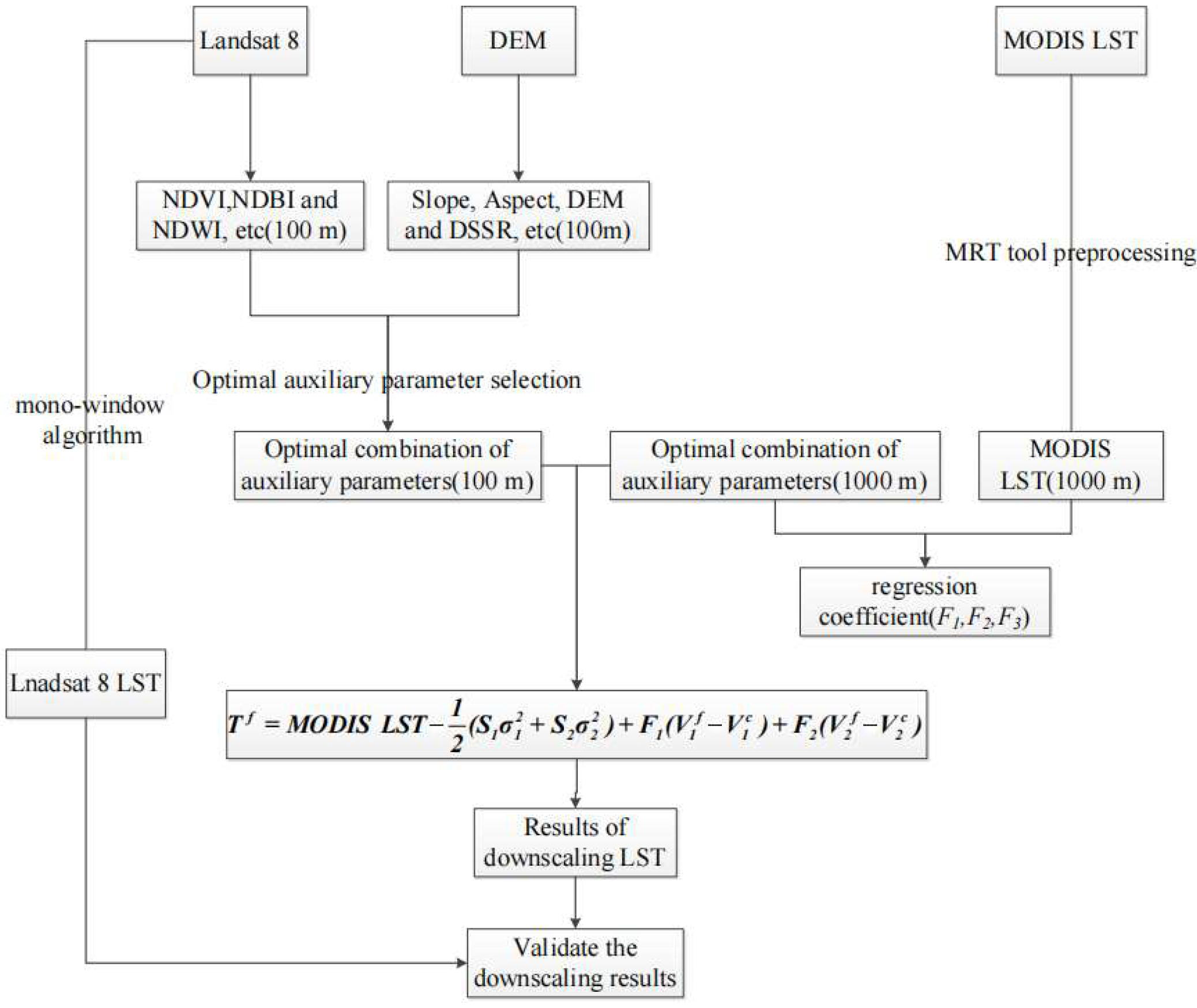
Figure 2 shows the flowchart of the LST downscaling algorithm in this study.
From the flowchart, this study is mainly divided into three parts: data preprocessing, establishment of the LST downscaling algorithm, and verification and analysis of LST downscaling results.
(1) Data preprocessing. This process includes preprocessing of Landsat 8, DEM, and MODIS LST data. The preprocessing of Landsat 8 and DEM data is mainly completed using ENVI 5.3 and ArcGis 10.2 software. The MODIS LST data are processed using the MODIS reprojection tool (MRT).
(2) LST downscaling algorithm. The method used in this study is the LST downscaling algorithm based on Taylor expansion proposed by Wang et al. in 2022 [
37]. Before that, the research on scale reduction methods was all based-on scale invariance, which made the surface temperature after scale reduction uncertain. The Taylor expansion algorithm estimates regression coefficients between LST and auxiliary parameters in a consistent scale. It is tested in three typical areas of different landscape with different auxiliary parameters, and the results are significantly improved compared to the traditional algorithm [
36]. Using this algorithm can reduce errors caused by scale issues and better verify and analyze the problems raised in this study. This algorithm considers the scale effect in the nonlinear relationship between LST and auxiliary parameters. The idea of the method is to derive the non-linear regression formula between LST and auxiliary parameters in low resolution, then downscale the LST to fine resolution using the first-order and second-order derivatives, as well as local differences and variances of auxiliary parameters. Therefore, in this study, we chose this algorithm as the downscaling method for rugged terrain areas. The details of the algorithm can be referenced in Wang et al. 2022 [
37], and the final downscaling formula is as follows:
where
are the variables in fine resolution pixel scale, and
are the variables in coarse resolution pixel scale:
refers to the LST;
refers to the geographical coordinates; and
refers to auxiliary parameter such as NDVI, NDBI, elevation, DSSR, etc. Subscript
represents the index of auxiliary parameter,
, while
is the number of auxiliary parameters.
is the partial derivative between LST and auxiliary parameter
in coarse resolution, and
is estimated with coarse resolution image data.
are variance of fine resolution auxiliary parameter within the coarse resolution pixel.
S is the empirical concavity factor, which is constant through the image, derived from Landsat LST. As we can see, the term
is the first-order correction, and the term
is the second-order correction for scale effect.
This study selected MODIS 1000 m spatial resolution LST data as the low spatial resolution LST data. Auxiliary parameters NDVI, NDBI are derived from the Landsat 8 image; elevation and slope are derived from DEM; and DSSR is derived from a combination of DEM, Landsat 8 image, and solar angle. According to the Taylor expansion proposed by Wang et al. [
37], we used the following formula for LST downscaling in this study.
where
and
were estimated and obtained at low spatial resolution (1000 m);
and
were estimated and obtained at high spatial resolution. In this study, it was obtained through Landsat 8 data.
represents auxiliary parameters such as NDVI, NDBI, DEM, and DSSR.
(3) Verification and analysis of LST downscaling results. Due to the limitations of field measurement data, remote sensing inverted LST is generally chosen as reference data to validate the downscaled results. Landsat 8 data are currently the best available data source for describing large-scale temperature spatial distribution. Therefore, this study chooses the LST inverted from Landsat 8 data as the reference data to verify the downscaled results. In terms of quantitative analysis, RMSE and MAE were selected as validation indicators to quantitatively verify the downscaled results. In addition, considering the possible bias in the inverted Landsat 8 LST, R2 is not affected by reference data bias and is an important indicator for algorithm evaluation.
4. LST Auxiliary Parameter Calculation in Complex Terrain Areas
To downscale LST in complex terrain areas, it is necessary to consider the influence of land cover types and terrain factors. NDVI, NDBI, and NDWI are widely used spectral indices to indicate land cover types. In addition, DSSR is also a significant influence factor for LST in complex terrain areas. Therefore, this study considers the influence of land cover types, terrain factors, and DSSR for LST downscaling in complex terrain areas.
4.1. Calculation of Land Cover Types
Most of study area a is forest, with a small amount of plowland in the southeast direction. The majority of study area b is farmland, grassland, and shrubbery, and there is a small amount of artificial land surface. NDVI can reflect the background influence of vegetation canopy and the growth status of vegetation. Some studies have shown that using the Building Index (NDBI) to extract impermeable surfaces is more effective. NDBI is insensitive to water bodies and shows a good fitting relationship with LST in all seasons. It has been widely used in current LST downscaling algorithm research. Therefore, this study chose the NDVI and NDBI as auxiliary parameters. In addition, considering that both study areas have water distribution, the water index NDWI is selected as an auxiliary parameter. In summary, considering the distribution of land cover types in the study area, NDVI, NDBI, and NDWI were selected as auxiliary parameters for LST downscaling modeling in this study.
4.2. Calculation of Terrain Factors
Slope and aspect are very important indicators for studying the terrain characteristics of mountainous areas. Slope is a measure of the specific rate of change in ground height, expressed as the angle between the normal direction and the vertical direction of a point on a surface. There are four methods for representing slope: fractional method, degree method, density method, and percentage method. The percentage method is the most commonly used method. Aspect is the angle between the projection of the normal direction on the horizontal plane and the true north direction, used to reflect the direction that the slope faces. Slope and aspect can be calculated using the grid method, usually in two ways: Ritter algorithm and Horn algorithm. The calculation of slope and aspect in this study was implemented using ArcGis 10.2 software, which uses the Horn algorithm for calculating slope and aspect.
It should be pointed out that the spatial resolution of DEM plays a crucial role in estimating terrain effect factors in the above analysis. To accurately estimate these factors, DEM data with a resolution equal to or higher than the spatial resolution of the sensor are required. The slope and aspect are obtained through DEM data in 30 m resolution, which is sufficiently fine, as our downscaled LST are in 100 m resolution.
Figure 3 and
Figure 4 respectively show the distribution maps of slope and aspect in two study areas.
From
Figure 3 and
Figure 4, it can be seen that the slope is represented as a percentage, with the aspect divided into ten directions: east, south, west, north, northeast, southeast, northwest, southwest, and flat. Generally, south, southwest, west, and northwest are considered sunny slopes; northeast, east, north, and southeast are shaded slopes.
4.3. Calculation of DSSR in Rugged Terrain
In rugged terrain areas, due to the influence of slope, aspect, and surrounding terrain, the distribution of shortwave radiation energy is uneven. The interaction of atmospheric effects and terrain effects ultimately leads to the spatio-temporal variability of DSSR over the rugged terrain area. Therefore, it is necessary to consider the relationship between LST and DSSR and select DSSR as an auxiliary parameter in LST downscaling modeling.
The DSSR in rugged areas is greatly affected by local terrain. As shown in
Figure 5, the radiation energy is divided into three parts: direct solar radiation, atmospheric scattering radiation, and reflected radiation of surrounding terrain [
43]. The total incident solar radiation on the rugged surface is the summation of the three parts [
42,
44,
45]:
where
E represents the total radiation received on the ground;
, and
represent direct solar radiation, sky scattered radiation, and surrounding terrain radiation, respectively.
Direct solar radiation is the main component of total solar radiation, and the calculation formula for direct solar radiation is as follows:
where
represents terrain shadows, a binary factor used to determine whether the target is directly exposed to the sun;
represents the direct solar irradiance received on the surface perpendicular to the light travel direction;
represents the localized solar zenith angle on slope, and its formula can be expressed as the following:
where,
and
represent the solar zenith angle and the solar azimuth angle, respectively;
S and A represent the slope and aspect of the slope, respectively.
On clear days, the parts of scattered radiation
and adjacent terrain radiation
are relatively much less than
and their calculation formula is much more complex. Therefore, this paper will not present their formula. Interested readers can refer to study [
2]. It is worth mentioning that the shortwave radiation calculated in this manuscript is not the actual shortwave radiation, as it does not account for atmospheric influence. For ease of understanding, the concept of shortwave radiation is used in this study.
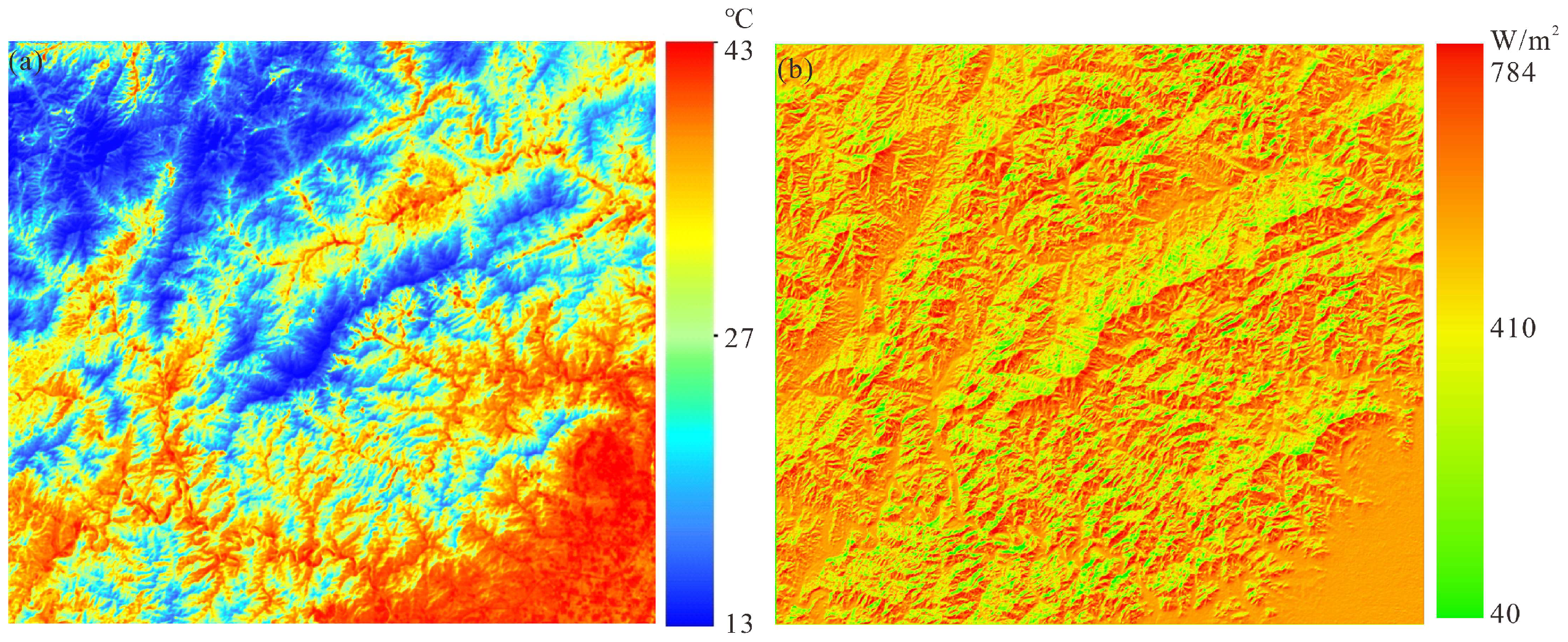
From
Figure 6 and
Figure 7, it can be seen that the distribution and trend of LST are not only related to elevation but also consistent with the texture details of DSSR. This indicates that shortwave radiation has a significant impact on LST in complex terrain areas, and research on LST in mountainous and other complex terrain areas requires the support of DSSR.
4.4. Selection of Auxiliary Parameters in Study Area
It is important to select appropriate auxiliary variables when downscaling LST with the scale factor method. Many factors such as vegetation, water, solar radiation, and land cover type need to be considered in the modeling process. However, it is unrealistic to select all the parameters, so this study selects the auxiliary parameters that have an evident correlation with LST. The study areas are mainly with rugged terrain, where the underlying surface properties (soil, vegetation conditions) and terrain conditions (slope, aspect, etc.) have a great impact on LST distribution. Considering the land cover type, NDVI can reflect the overall status of plant canopy in rugged terrain areas with lush vegetation. As a building index, the normalized difference built-up index (NDBI) can be used to extract impervious water surface. Although there is little urban area in the study areas, NDBI and LST still show a good linear relationship, so NDBI can be used as an auxiliary factor. Normalized difference water index (NDWI) is designed to highlight the water information on the land surface. In terms of topographic effect, the slope, aspect, and elevation (ELE) are commonly adopted to reflect the terrain characteristics of rugged area. Finally, DSSR is an important parameter affecting LST. In this study, LST downscaling is conducted by first selecting appropriate auxiliary parameter from NDVI, NDBI, NDWI, slope, aspect, ELE, and DSSR.
Table 2 shows the correlation results obtained by fitting different auxiliary parameters with LST in the four scene images of the two study areas.
As shown in
Table 2 for the four scene images, the slope and aspect have a small impact on LST, and the R
2 is quite small. In addition, previous studies have also pointed out that the average LST difference of different slope directions is less than 1 °C [
45]. Because there are not many water bodies and rivers in the study areas, the fitting effect between LST and NDWI is also poor. From the fitting results of two study areas, the fitting relationship between DEM and LST is pretty good. For NDVI and NDBI, their overall fitting effects are better in the four scenes data. Obvious seasonality is found in the fitting results of NDVI and NDBI. It can be seen that the fitting effect of NDVI and LST is better in summer (June and August), while the fitting effect of NDBI and LST is better in winter (October and December). Because of the lush vegetation in summer, the advantages of NDVI are more obvious, while in winter, the vegetation fades and bare soil is exposed, and the fitting effect of NDBI is better. In general, the fitting relationship between LST and DSSR is good in the two study areas. The fitting results of LST and DSSR also show seasonality; the R
2 is larger in winter than in summer. Affected by the solar altitude angle, the DSSR obtained in summer is larger than in winter, but because the dense vegetation canopy in summer blocks part of the solar radiation and the evaporation effect of vegetation is enhanced, effectively hindering the rise of LST. While the vegetation in winter is in the defoliation period, LST is greatly affected by DSSR, so the relationship between LST and DSSR is more prominent [
46]. This conclusion is based on the feature that the selected research area in this study is covered by vegetation. However, for other research areas, more rigorous experiments are needed to prove this conclusion. The seasonal impact of DSSR will be further explored in future studies.
Based on the above analysis, we chose NDVI, NDBI, ELE, and DSSR as auxiliary parameters for the next step of analysis, in which the combinations of the auxiliary parameters are evaluated.
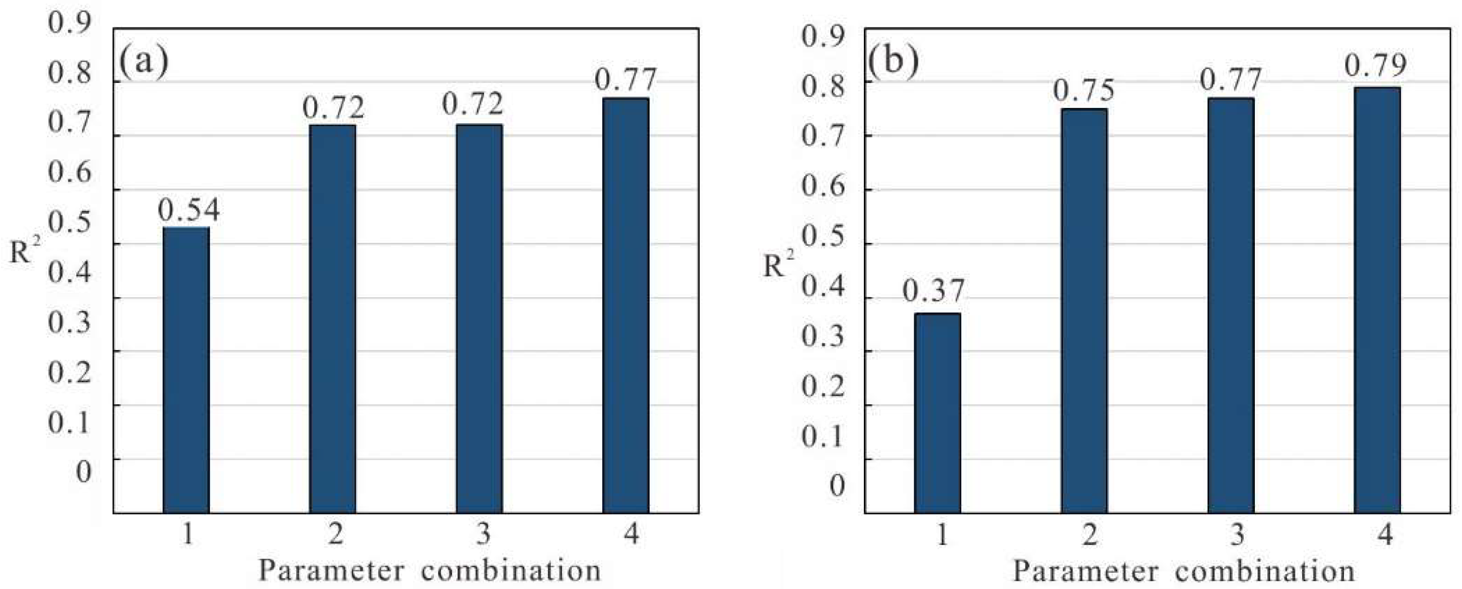
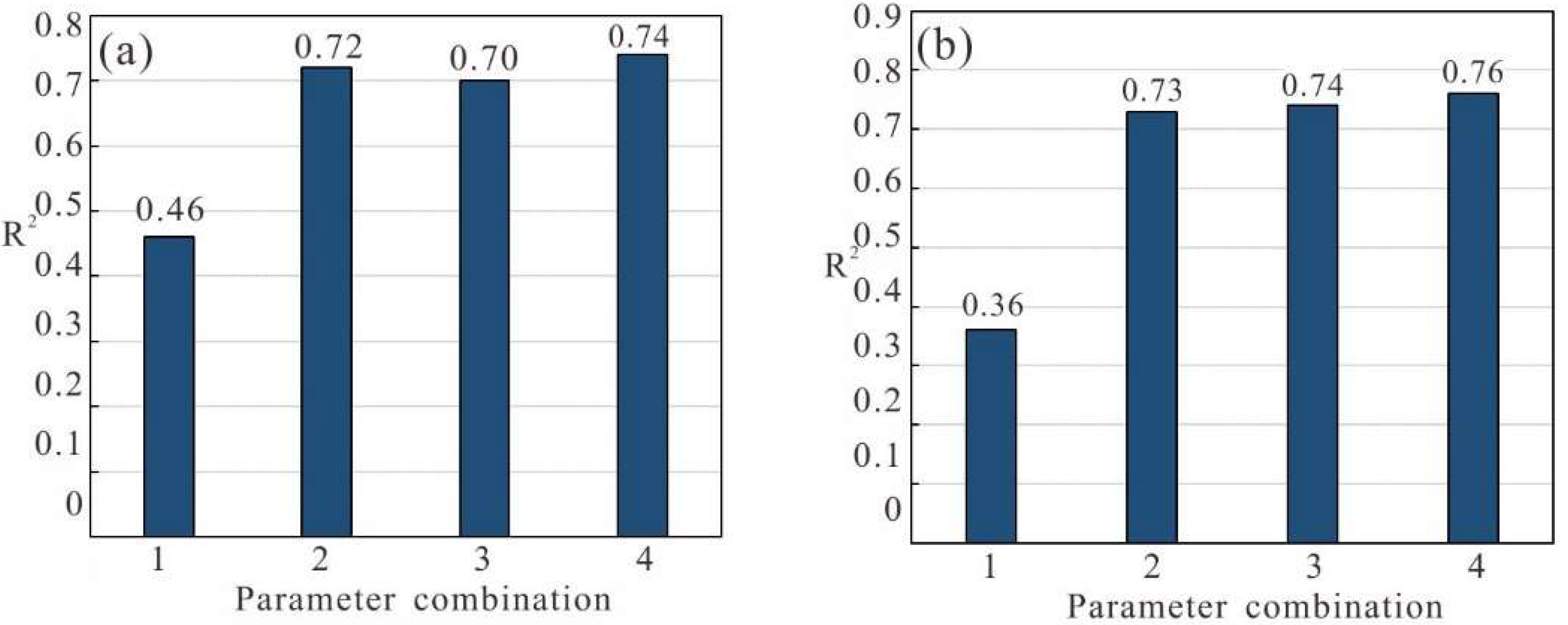
Figure 8 and
Figure 9 show the statistical results of least squares fitting R
2 of LST and different parameter combinations. The parameter combinations are as follows: combination 1, NDVI+NDBI; combination 2, NDVI+NDBI+DEM; combination 3, NDVI+NDBI+DSSR; and combination 4, NDVI+NDBI+DEM+DSSR.
It can be seen from
Figure 8 and
Figure 9 that the fitting result is poor for combination 1, which only uses the NDVI and the NDBI as auxiliary parameters and ignores the elevation factors and solar radiation. This will lead to large errors in the downscaling results and cannot meet the research need of LST. By considering the influence of ELE and DSSR, the accuracy will be greatly improved. Compared with the fitting results of combination 1 and combination 3, fitting R
2 has been greatly improved by adding DSSR. The results of combination 2 and combination 3 are relatively similar, while the R
2 of the results of combination 3 with DSSR is slightly higher than that of combination 2 with ELE. Moreover, the role of ELE is more important than that of DSSR in summer, while in winter, the advantage of DSSR is more evident. It can be seen from the above two figures that the best fitting result is obtained by using parameter combination 4, i.e., NDVI + NDBI + ELE + DSSR, which takes into account the influence of land cover, elevation, and solar radiation. Therefore, adding DSSR in the combination can get better fitting results. In the following study, the results of the LST downscaling algorithm based on the Taylor expansion model with each parameter combination as auxiliary parameters are verified and analyzed.
5. Results
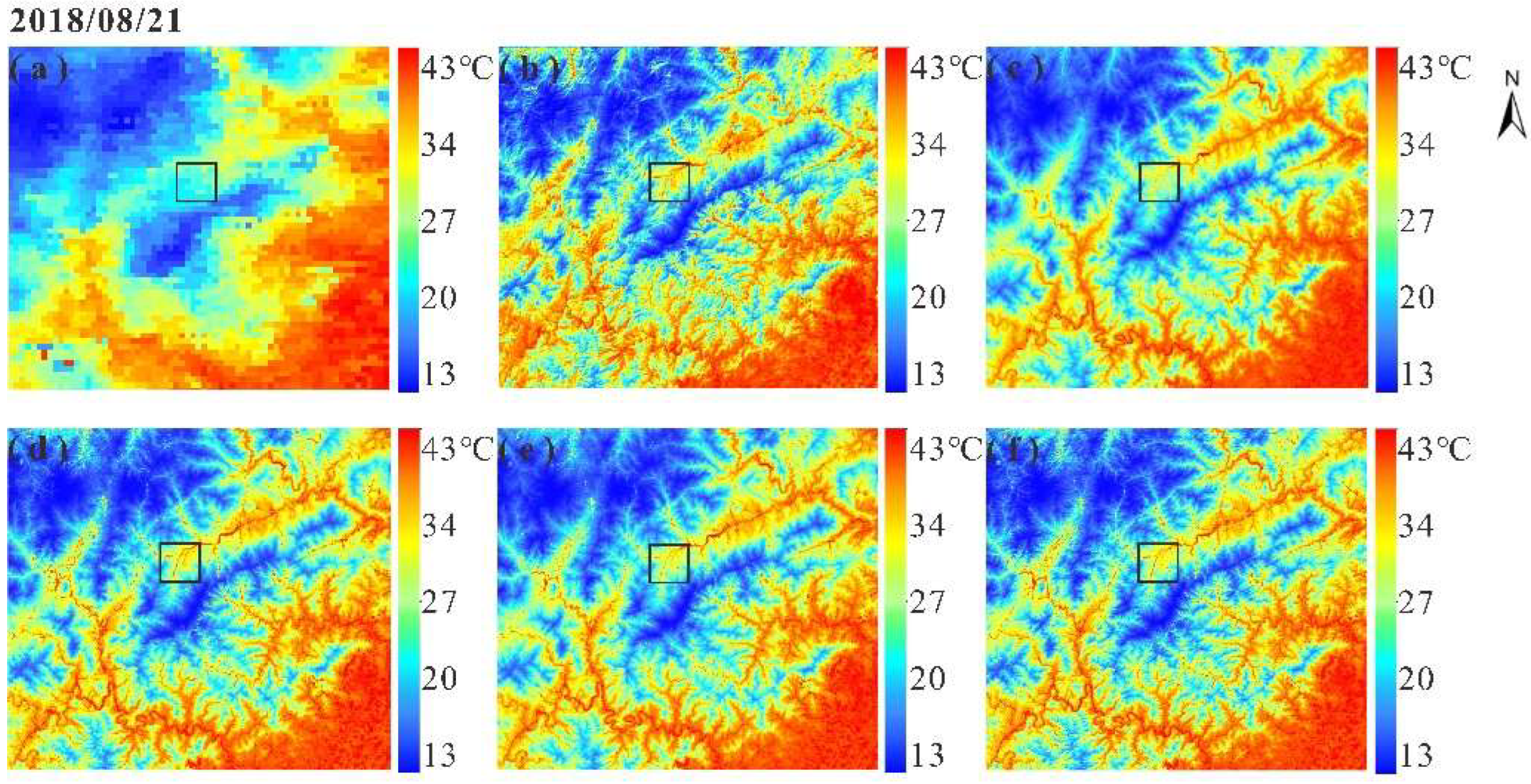
Figure 10 and
Figure 11 shows the downscaling results of study area a on 21 August 2018 and study area b on 13 October 2020, respectively. In
Figure 10 and
Figure 11, (a) and (b) show the MODIS LST with 1000 m spatial resolution and Landsat 8 LST with 100 m spatial resolution, respectively. The (c), (d), (e), and (f) represent the downscaling results based on auxiliary parameter combination 1, combination 2, combination 3, and Combination 4, with a spatial resolution of 100 m, respectively. It can be seen from the (a) in
Figure 10 and
Figure 11 that the MODIS LST data are not clear enough due to the low resolution, and the boundaries between the features are fuzzy. The MODIS LST with 1000 m spatial resolution cannot meet the research needs of the regional scale thermal environment. In addition,
Figure 10b and
Figure 11b are the LST retrieved from Landsat 8 data through the mono-window algorithm, which are used as the reference data in this study to verify the downscaling results. The trend of LST obtained by the downscaling algorithm is consistent with the reference LST of Landsat 8, with relatively clear spatial details.
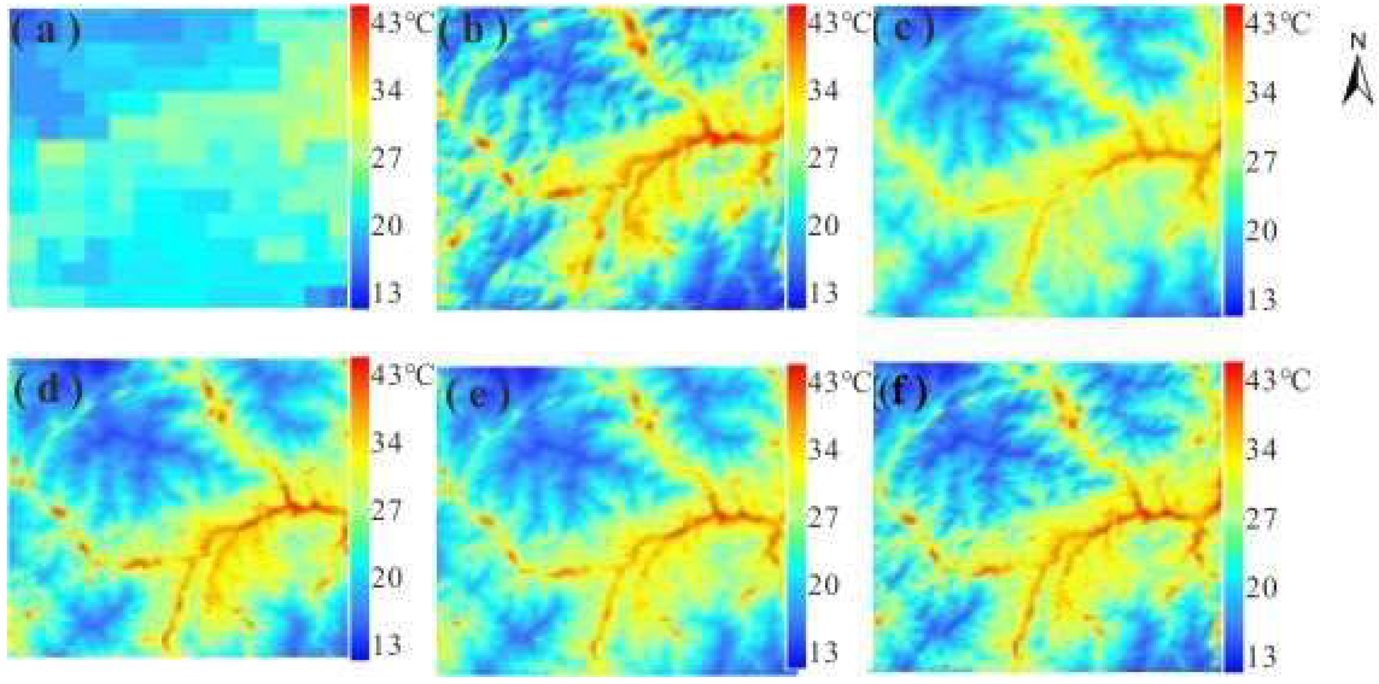
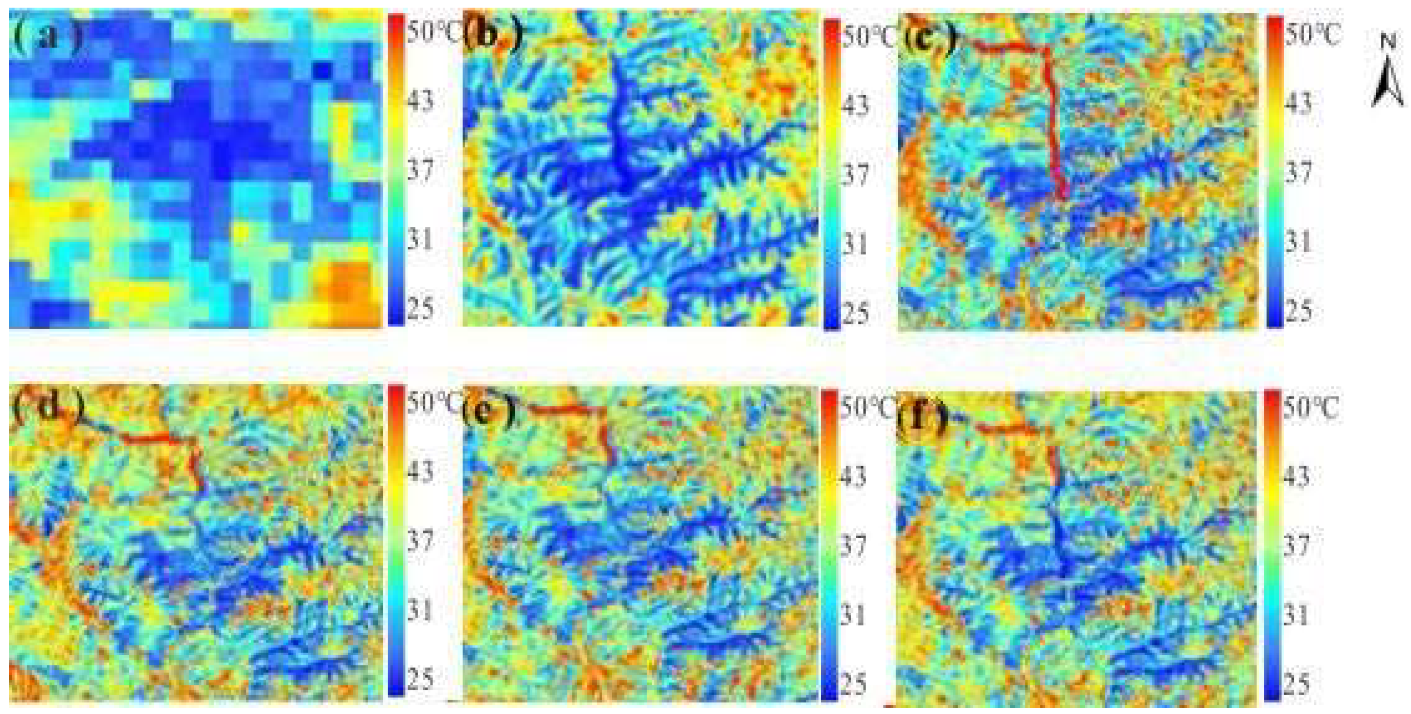
Figure 12 and
Figure 13 are the enlarged subsets of some details in
Figure 10 and
Figure 11. It can be seen from the enlarged detail images (
Figure 12 and
Figure 13) that the (f) is the closest to the Landsat 8 LST. Compared to the other images, the (c) is a little fuzzy. Especially in the area with higher altitude, the addition of DSSR makes the trend and texture of the mountain clearer. For study area b, the mountains in the enlarged figure are winding, and it can be seen in the enlarged figure that the details of the mountains are more similar to the reference Landsat 8 LST in (e) and (f), which were based on parameter combination 3 and combination 4, respectively. Through the observation of the detail map, it can be seen that adding DSSR as an auxiliary parameter will make the difference between the sunshine slope and the shadowed slope more obvious in the rugged terrain and more consistent with the reference image. Considering the land cover, elevation, and DSSR as scaling factors in the processing of LST downscaling can obtain LST with high accuracy and meet the requirements of monitoring the thermal environment of the rugged terrain area.
In this study, Landsat 8-retrieved LST by a mono-window algorithm is selected for quantitative analysis of downscaling results. Due to the difficulty of field measurement data and the need for accuracy verification of measured data, inversion LST is usually used as reference data to verify the downscaling results. Wang and Peng et al. analyzed and verified that the error between Landsat 8 LST and MODIS LST is less than 2 °C at 1000 m spatial resolution and less than the RMSE between ASTER and MODIS LST [
37,
38]. Therefore, LST retrieved by Landsat 8 by the mono-window algorithm is of high accuracy and can be used as reference data to verify the downscaling results. In this study, root mean square error (RMSE) and coefficient of determination (R
2) were selected to quantitatively verify and analyze the downscaling results. RMSE is a commonly used indicator to measure the difference between the predicted value and the actual value. Its core idea is to measure the error size of the prediction results and provide a concise numerical value to facilitate our understanding of the model’s accuracy. R
2 is the fitting metric of the linear regression model. This statistic represents the percentage of the variance of the dependent variable that the independent variables jointly explain. In this study, the statistics of R
2 and RMSE between the LST obtained through different parameter combinations and the reference LST are used.
Table 3 shows the RMSE and R
2 of the two study areas.
It can be seen from
Table 3 that the quantitative index response is basically consistent with the visual effect in
Figure 11,
Figure 12 and
Figure 13. The lowest RMSE and highest R
2 are obtained with parameter combination 4, with RMSE less than 1.5 °C and R
2 higher than 0.90. This indicates that the adding DSSR can improve the results of LST downscaling in rugged terrain areas. In addition, it is worth noting that in previous studies, which only considered elevation as an auxiliary parameter to downscale LST over rugged terrain areas, the results were better in summer than those in winter. However, when DSSR was added as an auxiliary parameter to the downscaling process, as in this study, LST downscaling accuracy was significantly improved in winter, and the best accuracy was obtained with combination 4 for both summer and winter.
6. Discussion
This study adds DSSR to the LST downscaling process, improves the accuracy of rugged terrain LST downscaling results, and provides a new prospect for thermal environment research over rugged terrain areas. This study can be regarded as a preliminary exploration of the impact of short-wave radiation on the downscaling of LST, and the method of this study has achieved good results in both study areas. This study laid the foundation for subsequent related research. The following discussion is about the current research and future research directions.
In this study, the main purpose was to investigate the influence of shortwave radiation on the scale reduction of surface temperature. Therefore, only different auxiliary parameters were considered for the comparative analysis of scale reduction. No comparative analysis was conducted with other methods. The method of this study has achieved good results in both study areas, but we are not conducting verification and analysis in more extreme terrain areas. In addition, the spatial resolution of 100 m is still relatively low for a topographic effect study, and it hinders the full exploration of DSSR’s effect on LST downscaling. Moreover, DSSR is a dynamic parameter that changes with solar angle.
Therefore, there are more specific recommendations for future research directions and applications of this improved downscaling approach in future study. First of all, select regions with more and more complex terrains and climates for more in-depth research. Study the effect of DSSR on more complex regions. Secondly, in this study, there is an impact of shortwave radiation as a parameter for downscaling results. The calculation of shortwave radiation is relatively simple, and the radiation data adopt a relatively basic method. For future research, the acquisition method of shortwave radiation can be improved to obtain more accurate radiation data of the short-wave range, providing more accurate data support for the establishment of the surface temperature scaling model. Then, we will use more LST downscaling methods to research the effect of DSSR in rugged terrain areas. In the end, finer spatial resolution and temporal dynamics of the thermal environment in rugged terrain areas should be analyzed based on in situ observation or sophisticated computer simulation data.
7. Conclusions
LST is an important parameter in the study of thermal environment and surface energy balance. However, the low spatial resolution of thermal infrared sensors limits the application of LST. LST downscaling is an effective method to obtain LST data with fine spatial and temporal resolution. In the study of LST downscaling, most of the study areas are cities and plains, and the study of rugged terrain areas is rare. In the few studies on rugged areas, LST downscaling is studied by adding elevation as the auxiliary factor. However, solar incident DSSR is a very important factor affecting surface temperature and is very heterogenous in rugged terrain. Therefore, in this study, DSSR is taken as one of the auxiliary factors for LST downscaling in rugged terrain areas, and the results of LST downscaling in rugged terrain areas are verified.
In this study, we selected two rugged terrain areas for an LST downscaling study. We investigated the auxiliary parameters that have evident correlation with LST in rugged areas and finally chose NDVI, NDBI, elevation, and DSSR as the candidate auxiliary parameters for LST downscaling. In addition, we compared and analyzed the downscaling results with different parameter combinations. Through the analysis, we found that the downscaling results with added DSSR are considerably improved. This shows that considering the influence of solar radiation is beneficial to the improvement of downscaling accuracy. Moreover, adding DSSR can improve the results in autumn and winter more significantly than in summer, which also improves the disadvantages of the previous downscaling algorithm.
This study adds DSSR to the LST downscaling process, improves the accuracy of rugged terrain LST downscaling results, and provides a new prospect for thermal environment research over rugged terrain area. In this study, the main purpose was to investigate the influence of short-wave radiation on the scale reduction of surface temperature. Therefore, only different auxiliary parameters were considered for the comparative analysis of scale reduction, and no comparative analysis was conducted with other methods. In addition, the spatial resolution of 100 m is still relatively low for a topographic effect study, and it hinders the full exploration of DSSR’s effect on LST downscaling. Moreover, DSSR is a dynamic parameter that changes with solar angle. Therefore, there are more specific recommendations for future research directions and applications of this improved downscaling approach in future study. First of all, select regions with more and more complex terrains and climates for more in-depth research. Study the effect of DSSR on more complex regions. Secondly, in this study, the calculation of shortwave radiation data adopts a relatively basic method. For future research, the acquisition method of shortwave radiation can be improved to obtain more accurate radiation data of the short-wave range, providing more accurate data support for the establishment of the surface temperature scaling model. Then we will use more LST downscaling methods to research the effect of DSSR in rugged terrain areas. In the end, finer spatial resolution and temporal dynamics of the thermal environment in rugged terrain areas should be analyzed based on in situ observation or sophisticated computer simulation data.
Author Contributions
Conceptualization, Q.L.; methodology, software, S.W.; validation, J.C.; writing—original draft preparation, Q.L. and S.W.; writing, review, and editing, S.W., J.C. and Q.L. All authors have read and agreed to the published version of the manuscript.
Funding
This research was supported by Open Fund of State Key Laboratory of Remote Sensing Science (Grant No. OFSLRSS202414), and Hubei Second Normal University talent introduction research project (Grant No. ESRC20240009).
Data Availability Statement
The raw data supporting the conclusions of this article will be made available by the authors on request.
Acknowledgments
The authors would like to thank the contributions of the anonymous reviewers and the Institute of Remote Sensing and Digital Earth Chinese Academy of Sciences. The authors would also like to thank NASA for providing the satellite data and insightful comments that helped significantly improve this manuscript.
Conflicts of Interest
The authors declare no conflicts of interest. The funders had no role in the design of the study; in the collection, analyses, or interpretation of data; in the writing of the manuscript, or in the decision to publish the results.
References
- Malakar, N.K.; Hulley, G.C.; Hook, S.J.; Laraby, K.; Cook, M.; Schott, J.R. An Operational Land Surface Temperature Product for Landsat Thermal Data: Methodology and Validation. IEEE Trans. Geoence Remote Sens. 2018, 56, 5717–5735. [Google Scholar] [CrossRef]
- Amazirh, A.; Merlin, O.; Er-Raki, S.; Gao, Q.; Rivalland, V.; Malbeteau, Y.; Khabba, S.; Escorihuela, M.J. Retrieving surface soil moisture at high spatio-temporal resolution from a synergy between Sentinel-1 radar and Landsat thermal data: A study case over bare soil. Remote Sens. Environ. Interdiscip. J. 2018, 211, 321–337. [Google Scholar] [CrossRef]
- Liu, S.; Pan, X.; Yuan, J.; Tansey, K.; Yang, Z.; Wang, Z.; Ding, X.; Liu, Y.; Yang, Y. A non-parametric method combined with surface flux equilibrium for estimating terrestrial evapotranspiration: Validation at eddy covariance sites. J. Hydrol. 2024, 631, 130682. [Google Scholar]
- Li, Z.L.; Tang, B.H.; Wu, H.; Ren, H.Z.; Yan, G.J.; Wan, Z.M. Satellite-derived land surface temperature: Current status and perspectives. Elsevier 2013, 131, 14–37. [Google Scholar] [CrossRef]
- Wang, Z.C.; Pan, X.; Ding, X.; Rufat, G.; Yang, Z.; Yuan, J.; Zhou, Y.L.; Liu, S.; Ma, W.Q.; Liu, Y.B.; et al. Intercomparison of temporal upscaling strategies for daily evapotranspiration estimation from the perspective of land surface temperature. J. Hydrol. 2025, 660 Pt B, 133461. [Google Scholar] [CrossRef]
- Zhou, J.; Chen, Y.; Zhang, X.; Zhan, W.F. Modelling the diurnal variations of urban heat islands with multi-source satellite data. Int. J. Remote Sens. 2013, 34, 21. [Google Scholar] [CrossRef]
- Hu, J.; Yang, Y.; Pan, X.; Zhan, W.F.; Wang, Y. Analysis of the Spatial and Temporal Variations of Land Surface Temperature Based on Local Climate Zones: A Case Study in Nanjing, China. IEEE J. Sel. Top. Appl. Earth Obs. Remote Sens. 2019, 12, 4213–4223. [Google Scholar] [CrossRef]
- Li, S.; Wang, X.; Xie, A.; Ma, B. Downscaling MODIS Land Surface Temperatures Using Multilayer Perceptron Model. Res. Environ. Sci. 2017, 30, 1889–1897. [Google Scholar]
- Yao, Y.; Chen, X.; Qian, J. Research progress on the thermal environment of the urban surface. Shengtai Xuebao Acta Ecol. Sin. 2018, 38, 1134–1147. [Google Scholar]
- Julien, M.; Olivier, H.; Simon, J.; Jean-Louis, R.; Philippe, G. Quantifying Thermal Infra-Red directional anisotropy using Master and Landsat-8 simultaneous acquisitions. Remote Sens. Environ. 2023, 297, 113765. [Google Scholar]
- Sobrino, J.A.; Oltra-Carrió, R.; Sòria, G.; Bianchi, R.; Paganini, M. Impact of spatial resolution and satellite overpass time on evaluation of the surface urban heat island effects. Remote Sens. Environ. 2012, 117, 50–56. [Google Scholar] [CrossRef]
- Luo, J.; Li, X.; Ma, R.; Li, F.; Duan, H.T.; Hu, W.P.; Qin, B.Q. Applying remote sensing techniques to monitoring seasonal and interannual changes of aquatic vegetation in Taihu Lake, China. Ecol. Indic. 2016, 60, 503–513. [Google Scholar] [CrossRef]
- Mo, Y.; Momen, B.; Kearney, M.S. Quantifying moderate resolution remote sensing phenology of Louisiana coastal marshes. Ecol. Model. 2015, 312, 191–199. [Google Scholar] [CrossRef]
- Fisher, J.I.; Mustard, J.F. Cross-scalar satellite phenology from ground, Landsat, and MODIS data. Remote Sens. Environ. 2007, 109, 261–273. [Google Scholar] [CrossRef]
- Wu, M.; Zhang, X.; Huang, W.; Niu, Z.; Wang, C.Y.; Li, W.; Hao, P.Y. Reconstruction of Daily 30 m Data from HJ CCD, GF-1 WFV, Landsat, and MODIS Data for Crop Monitoring. Remote Sens. 2015, 7, 16293–16314. [Google Scholar] [CrossRef]
- Ha, W.; Gowda, P.H.; Howell, T.A. A review of downscaling methods for remote sensing-based irrigation management: Part I. Irrig. Ence 2013, 31, 831–850. [Google Scholar] [CrossRef]
- Weng, Q.; Fu, P. Modeling diurnal land temperature cycles over Los Angeles using downscaled GOES imagery. ISPRS J. Photogramm. Remote Sens. 2014, 97, 78–88. [Google Scholar] [CrossRef]
- Bonafoni, S. Downscaling of Landsat and MODIS Land Surface Temperature Over the Heterogeneous Urban Area of Milan. IEEE J. Sel. Top. Appl. Earth Obs. Remote Sens. 2016, 9, 2019–2027. [Google Scholar] [CrossRef]
- Yang, G.; Pu, R.; Zhao, C.; Huang, W.J.; Wang, J.H. Estimation of subpixel land surface temperature using an endmember index based technique: A case examination on ASTER and MODIS temperature products over a heterogeneous area. Remote Sens. Environ. 2011, 115, 1202–1219. [Google Scholar] [CrossRef]
- Honda, T.; Miyoshi, T.; Lien, G.Y.; Nishizawa, S.; Yoshida, R.; Adachi, S.A. Assimilating All-Sky Himawari-8 Satellite Infrared Radiances: A Case of Typhoon Soudelor (2015). Mon. Weather Rev. 2018, 146, 213–229. [Google Scholar] [CrossRef]
- Gao, L.; Zhan, W.; Huang, F.; Huang, F.; Quan, J.L.; Lu, X.M.; Wang, F. Localization or Globalization? Determination of the Optimal Regression Window for Disaggregation of Land Surface Temperature. IEEE Trans. Geosci. Remote Sens. 2017, 55, 477–490. [Google Scholar] [CrossRef]
- Zhan, W.; Chen, Y.; Zhou, J.; Wang, J.F.; Liu, W.Y.; Voogt, J.; Zhu, X.L.; Quan, J.L.; Li, J. Disaggregation of remotely sensed land surface temperature: Literature survey, taxonomy, issues, and caveats. Remote Sens. Environ. 2013, 131, 119–139. [Google Scholar] [CrossRef]
- Wu, P.; Yin, Z.; Zeng, C.; Duan, S.B.; Ma, X.S. Spatially Continuous and High-resolution Land Surface Temperature: A Review of Reconstruction and Spatiotemporal Fusion Techniques. IEEE Geosci. Remote Sens. Mag. 2019, 1909, 09316. [Google Scholar] [CrossRef]
- Li, Y.; Qu, J.; Dong, W.; Zheng, Y.X. Hyperspectral pan sharpening via improved PCA approach and optimal weighted fusion strategy. Neurocomputing 2018, 315, 371–380. [Google Scholar] [CrossRef]
- Carper, W.J.; Lillesand, T.M.; Kiefer, P.W. The use of intensity-hue-saturation transformations for merging SPOT panchromatic and multispectral image data. Photogramm. Eng. Remote Sens. 1990, 56, 459–467. [Google Scholar]
- Nunez, J.; Otazu, X.; Fors, O.; Prades, A.; Pala, V.; Arbiol, R. Multiresolution-based image fusion with additive wavelet decomposition. IEEE Trans. Geosci. Remote Sens. 1999, 37, 1204–1211. [Google Scholar] [CrossRef]
- Feng, G.; Masek, J.G.; Schwaller, M.R.; Hall, F. On the Blending of the Landsat and MODIS Surface Reflectance: Predicting Daily Landsat Surface Reflectance. IEEE Trans. Geosci. Remote Sens. 2006, 44, 2207–2218. [Google Scholar] [CrossRef]
- Wu, M.Q.; Jie, W.; Niu, Z.; Zhao, Y.Q.; Wang, C.Y. A model for spatial and temporal data fusion. J. Infrared Millim. Waves 2012, 31, 80–84. [Google Scholar] [CrossRef]
- Zhu, X.; Helmer, E.; Gao, F.; Liu, D.; Chen, J.; Lefsky, M.A. A flexible spatiotemporal method for fusing satellite images with different resolutions. Remote Sens. Environ. Interdiscip. J. 2016, 172, 165–177. [Google Scholar] [CrossRef]
- Kustas, W.P.; Norman, J.M.; Anderson, M.C.; French, A.N. Estimating subpixel surface temperatures and energy fluxes from the vegetation index-radiometric temperature relationship. Remote Sens. Environ. 2003, 85, 429–440. [Google Scholar] [CrossRef]
- Agam, N.; Kustas, W.P.; Anderson, M.C.; Li, F.; Neale, C.M. A vegetation index based technique for spatial sharpening of thermal imagery. Remote Sens. Environ. 2007, 107, 545–558. [Google Scholar] [CrossRef]
- Agam, N.; Kustas, W.P.; Anderson, M.C. Utility of thermal image sharpening for monitoring field-scale evapotranspiration over rainfed and irrigated agricultural regions. Geophys. Res. Lett. 2008, 35, 196–199. [Google Scholar] [CrossRef]
- Cheng, J.; Yang, D.; Qie, K. Analysis of land surface temperature drivers in Beijing’s central urban area across multiple spatial scales: An explainable ensemble learning approach. Energy Build. 2025, 338, 115704. [Google Scholar] [CrossRef]
- Zakšek, K.; Oštir, K. Downscaling land surface temperature for urban heat island diurnal cycle analysis. Remote Sens. Environ. 2012, 117, 114–124. [Google Scholar] [CrossRef]
- Zhu, S.; Guan, H.; Millington, A.C.; Li, F.; Colaizzi, P.D. Disaggregation of land surface temperature over a heterogeneous urban and surrounding suburban area: A case study in Shanghai, China. Int. J. Remote Sens. 2013, 34, 1707–1723. [Google Scholar] [CrossRef]
- Eswar, R.; Sekhar, M.; Bhattacharya, B.K. Disaggregation of LST over India: Comparative analysis of different vegetation indices. Int. J. Remote Sens. 2016, 37, 1035–1054. [Google Scholar] [CrossRef]
- Wang, S.; Luo, Y.; Li, M. A Taylor Expansion Algorithm for Spatial Downscaling of MODIS Land Surface Temperature. IEEE Trans. Geosci. Remote Sens. 2022, 60, 1–17. [Google Scholar] [CrossRef]
- Peng, Y.; Li, W.; Luo, X.; Li, M.Y.; Yang, K.X.; Liu, Q.; Li, X.H. A Geographically and Temporally Weighted Regression Model for Spatial Downscaling of MODIS Land Surface Temperatures Over Urban Heterogeneous Regions. IEEE Trans. Geosci. Remote Sens. 2019, 57, 5012–5027. [Google Scholar] [CrossRef]
- Wang, S.; Luo, X.; Peng, Y. Spatial Downscaling of MODIS Land Surface Temperature Based on Geographically Weighted Autoregressive Model. IEEE J. Sel. Top. Appl. Earth Obs. Remote Sens. 2020, 13, 2532–2546. [Google Scholar] [CrossRef]
- Zhou, T.Y.; Wang, Z.H.; Qin, H.Y.; Zeng, Y.Q. Remote sensing extraction of geothermal anomaly based on terrain effect correction. J. Remote Sens. 2020, 24, 265–276. [Google Scholar] [CrossRef]
- Cheng, Y.; Wu, H.; Li, L.Z.; Göttsche, F.M.; Zhang, X.X.; Li, X.J.; Zhang, H.Y.; Li, Y.T. A robust framework for accurate land surface temperature retrieval: Integrating split-window into knowledge-guided machine learning approach. Remote Sens. Environ. 2025, 318, 114609. [Google Scholar] [CrossRef]
- Mousivand, A.; Verhoef, W.; Massimo, M.; Ben, G. Modeling Top of Atmosphere Radiance over Heterogeneous Non-Lambertian Rugged Terrain. Remote Sens. 2015, 7, 8019–8044. [Google Scholar] [CrossRef]
- Lu, X.; Wang, R.; Li, J.; Lyu, S.; Zhang, J.; Wang, Q.; Chi, W.; Zhong, R.; Chen, C.; Wu, X.; et al. Exposure-lag response of surface net solar radiation on lung cancer incidence: A global time-series analysis. Transl. Lung Cancer Res. 2024, 13, 2524–2537. [Google Scholar] [CrossRef] [PubMed]
- Wen, J.; Liu, Q.; Xiao, Q.; Liu, Q.; You, D.; Hao, D. Characterizing Land Surface Anisotropic Reflectance over Rugged Terrain: A Review of Concepts and Recent Developments. Remote Sens. 2018, 10, 370. [Google Scholar] [CrossRef]
- Wu, S.; Wen, J.; You, D.; Zhang, H.; Liu, Q. Algorithms for Calculating Topographic Parameters and Their Uncertainties in Downward Surface Solar Radiation (DSSR) Estimation. IEEE Geosci. Remote Sens. Lett. 2018, 15, 1149–1153. [Google Scholar] [CrossRef]
- Liu, B.; Ma, L.; Rong, X.; Su, J.Z.; Yan, Y.H.; Hua, L.J.; Tang, Y.L. High-resolution Model for Seasonal Prediction of Surface Shortwave Radiation in China. J. Appl. Meteorol. Sci. 2022, 33, 341–352. [Google Scholar]
Figure 1.
The false color image of Study area a and Study area b generated from Landsat 8 data.
Figure 1.
The false color image of Study area a and Study area b generated from Landsat 8 data.
Figure 2.
Flowchart of the LST downscaling algorithm.
Figure 2.
Flowchart of the LST downscaling algorithm.
Figure 3.
Distribution of slope direction in study area a, (a): slope gradient; (b): slope direction.
Figure 3.
Distribution of slope direction in study area a, (a): slope gradient; (b): slope direction.
Figure 4.
Distribution of slope direction in study area b, (a): slope gradient; (b): slope direction.
Figure 4.
Distribution of slope direction in study area b, (a): slope gradient; (b): slope direction.
Figure 5.
Surface solar incident radiation over rugged terrain.
Figure 5.
Surface solar incident radiation over rugged terrain.
Figure 6.
Distribution map of LST and DSSR in study area a, (a): LST; (b): DSSR.
Figure 6.
Distribution map of LST and DSSR in study area a, (a): LST; (b): DSSR.
Figure 7.
Distribution map of LST and DSSR in study area b, (a): LST; (b): DSSR.
Figure 7.
Distribution map of LST and DSSR in study area b, (a): LST; (b): DSSR.
Figure 8.
The R2 statistical data of LST and different parameter combinations in study area a ((a): 21 August 2018, (b): 13 October 2020).
Figure 8.
The R2 statistical data of LST and different parameter combinations in study area a ((a): 21 August 2018, (b): 13 October 2020).
Figure 9.
The R2 statistical data of LST and different parameter combinations in study area b ((a): 27 June 2017, (b): 20 December 2017).
Figure 9.
The R2 statistical data of LST and different parameter combinations in study area b ((a): 27 June 2017, (b): 20 December 2017).
Figure 10.
Downscaling results for study area a on 21 August 2018. (a): MODIS LST with 1000 m spatial resolution; (b): Landsat 8 LST with 100 m spatial resolution, respectively. The (c–f) represent the downscaling results based on auxiliary parameter combination 1, combination 2, combination 3, and combination 4, with a spatial resolution of 100 m, respectively.
Figure 11.
Downscaling results for study area b on 27 June 2017. (a): MODIS LST with 1000 m spatial resolution; (b): Landsat 8 LST with 100 m spatial resolution, respectively. The (c–f) represent the downscaling results based on auxiliary parameter combination 1, combination 2, combination 3, and combination 4, with a spatial resolution of 100 m, respectively.
Figure 12.
Enlarged view of some area details in
Figure 11. (
a): MODIS LST with 1000 m spatial resolution; (
b): Landsat 8 LST with 100 m spatial resolution, respectively. The (
c–
f) represent the downscaling results based on auxiliary parameter combination 1, combination 2, combination 3, and combination 4, with a spatial resolution of 100 m, respectively.
Figure 13.
Enlarged view of some area details in
Figure 12. (
a): MODIS LST with 1000 m spatial resolution; (
b): Landsat 8 LST with 100 m spatial resolution, respectively. The (
c–
f) represent the downscaling results based on auxiliary parameter combination 1, combination 2, combination 3, and combination 4, with a spatial resolution of 100 m, respectively.
Table 1.
Satellite data and their acquisition time.
Table 1.
Satellite data and their acquisition time.
| Study Areas | Acquisition Time
(Landsat 8 Data) | Acquisition Time
(MODIS LST Data) |
|---|
| a | 2018/08/21 02:59:10 | 2018/08/21 03:45:00 |
| 2016/10/13 03:00:02 | 2016/10/13 03:20:00 |
| b | 2017/06/27 03:25:22 | 2017/06/27 03:45:00 |
| 2017/12/20 03:25:48 | 2017/12/20 03:35:00 |
Table 2.
R2 of LST and auxiliary parameters.
Table 2.
R2 of LST and auxiliary parameters.
| Study Area | Data | NDVI | NDBI | NDWI | Slope | Aspect | ELE | DSSR |
|---|
| a | 2018.08.21 | 0.45 | 0.30 | 0.036 | 0.00709 | 0.0359 | 0.5802 | 0.2178 |
| 2020.10.13 | 0.29 | 0.34 | 0.087 | 0.00999 | 0.0733 | 0.6215 | 0.5632 |
| b | 2017.06.27 | 0.53 | 0.38 | 0.053 | 0.00787 | 0.0693 | 0.4912 | 0.2318 |
| 2017.12.20 | 0.26 | 0.35 | 0.055 | 0.00624 | 0.0392 | 0.5261 | 0.5493 |
Table 3.
The LST downscaling accuracy statistic in the two study areas.
Table 3.
The LST downscaling accuracy statistic in the two study areas.
| Study Area | Parameter Combinations | 1 | 2 | 3 | 4 |
|---|
| Index | Data | RMSE
(°C) | R2 | RMSE
(°C) | R2 | RMSE
(°C) | R2 | RMSE
(°C) | R2 |
|---|
| a | 21 August 2018 | 2.79 | 0.73 | 1.31 | 0.90 | 1.27 | 0.91 | 1.12 | 0.92 |
| 13 October 2020 | 3.14 | 0.68 | 1.34 | 0.90 | 1.31 | 0.90 | 1.09 | 0.93 |
| b | 27 June 2017 | 2.53 | 0.76 | 1.03 | 0.93 | 1.03 | 0.92 | 0.99 | 0.94 |
| 20 December 2017 | 3.01 | 0.70 | 1.14 | 0.92 | 1.15 | 0.92 | 1.02 | 0.94 |
| Disclaimer/Publisher’s Note: The statements, opinions and data contained in all publications are solely those of the individual author(s) and contributor(s) and not of MDPI and/or the editor(s). MDPI and/or the editor(s) disclaim responsibility for any injury to people or property resulting from any ideas, methods, instructions or products referred to in the content. |
© 2025 by the authors. Licensee MDPI, Basel, Switzerland. This article is an open access article distributed under the terms and conditions of the Creative Commons Attribution (CC BY) license (https://creativecommons.org/licenses/by/4.0/).


