Spatial Downscaling of Sea Level Anomaly Using a Deep Separable Distillation Network

Abstract

The use of high-resolution sea level anomaly (SLA) data in climate change research and ocean forecasting has become increasingly important. However, existing datasets often lack the fine spatial resolution required for capturing mesoscale ocean processes accurately. This has led to the development of conventional deep learning models for SLA spatial downscaling, but these models often overlook spatial disparities between land and ocean regions and do not adequately address the spatial structures of SLA data. As a result, their accuracy and structural consistency are suboptimal. To address these issues, we propose a Deep Separable Distillation Network (DSDN) that integrates Depthwise Separable Distillation Blocks (DSDB) and a Landmask Contextual Attention Mechanism (M_CAMB) to achieve efficient and accurate spatial downscaling. The M_CAMB employs geographically-informed land masks to enhance the attention mechanism, prioritizing ocean regions. Additionally, we introduce a novel Pixel-Structure Loss (PSLoss) to enforce spatial structure constraints, significantly improving the structural fidelity of the SLA downscaling results. Experimental results demonstrate that DSDN achieves a root mean square error (RMSE) of 0.062 cm, a peak signal-to-noise ratio (PSNR) of 42.22 dB, and a structural similarity index (SSIM) of 0.976 in SLA downscaling. These results surpass those of baseline models and highlight the superior precision and structural consistency of DSDN.

1. Introduction

Sea level anomaly (SLA) is a crucial parameter for monitoring the dynamic marine environment and is used in various applications such as understanding ocean circulation variability, predicting extreme climate events like El Ni no, and assessing global sea level rise trends [1,2,3]. However, the spatial resolution of SLA data derived from satellite altimeters is typically 1/4° (approximately 25 km), which is insufficient for high-precision oceanographic research [4]. For example, Copernicus/AVISO now provides gridded SLA products at 1/8° resolution in historical and near-real-time datasets, offering improved spatial detail; nonetheless, even these may not fully capture finer mesoscale processes. Applications such as fine-scale modeling of nearshore waters and precise detection of mesoscale eddies (10–100 km), therefore, require even higher-resolution SLA products (e.g., 1/16°) [5]. Mesoscale eddies contribute over 90% of the global ocean kinetic energy flux, but their spatial scales (typically below 100 km) mean that 1/4° data cannot accurately resolve their boundary geometries and three-dimensional structures [6]. Increasing SLA resolution to 1/16° has been shown to improve eddy identification accuracy by approximately 30%, significantly enhancing the quantification of oceanic material transport, including heat and salinity [7]. Moreover, high-resolution SLA data are essential for analyzing air–sea interactions, such as the upper-ocean response to typhoons, and for initializing nearshore circulation models [8].

However, conventional approaches to enhancing SLA resolution exhibit notable limitations. Traditional interpolation techniques (e.g., bilinear interpolation) fail to preserve high-frequency details of the physical field, resulting in over-smoothed reconstructions [9]. Likewise, dynamic downscaling using regional ocean models (e.g., ROMS) can capture small-scale processes but incur high computational cost and require complex parameterizations [10]. For example, gridded SLA at 1/4° produced from multiple altimeters still misses many mesoscale eddies, highlighting the shortcomings of simple interpolation. These challenges motivate data-driven downscaling: statistical methods establish empirical relationships between large-scale predictors and local variables to generate fine-scale fields. In practice, statistical downscaling has been widely used in climate impact studies [11], but its accuracy depends on the quality of training data and predictors. With the rapid expansion of big Earth datasets and improvements in computational capabilities, deep learning has shown great potential to advance statistical downscaling [12]. In particular, convolutional neural networks (CNNs), with their ability to automatically extract spatial features, have become a cornerstone of downscaling approaches [13]. CNNs’ multi-layer architectures can capture complex nonlinear mappings from coarse to fine scales, often outperforming traditional statistical techniques [14]. However, even with these advances, developing efficient and physically consistent downscaling methods remains a priority in ocean remote sensing [15].

Recent advancements in deep learning have provided innovative solutions to the challenges of statistical downscaling [16]. For instance, the DeepSD framework [17] couples low-resolution climate model outputs with high-resolution topography to improve precipitation downscaling. In the oceanographic context, Generative Adversarial Networks (GANs) have been used to downscale 1° sea surface temperature (SST) fields to 0.25°, thereby improving the timeliness of El Ni no index predictions [18]. Similarly, Martin et al. [19] employed a ConvLSTM model to integrate multi-temporal satellite altimeter data, achieving dynamic reconstruction of submesoscale (less than 10 km) sea surface height with high fidelity (correlation 0.90 compared to Argo float data). These examples demonstrate that deep neural networks can enhance the spatial resolution of ocean surface fields beyond traditional methods.

Despite these advances, most current deep learning approaches rely on single-modality inputs and face significant limitations. Conventional CNN models often neglect the spatial heterogeneity between land and ocean regions when processing marine data, leading to suboptimal feature representation for variables such as SLA [9]. They also involve high computational complexity, which can be a bottleneck for large-scale applications [20]. In addition, the spatiotemporal distribution of SLA is synergistically regulated by multiple oceanographic factors—such as sea surface wind fields, currents, and temperature. For example, seasonal and interannual SLA variations in the South China Sea are coupled with wind stress curl, the Kuroshio Current, and ENSO-related heat content changes [21]. Integrating multi-source remote sensing data (e.g., along-track altimetry, scatterometry, and infrared SST) can effectively capture these coupled processes [22]. Indeed, combining altimetry with high-resolution SST imagery has been shown to produce more accurate, higher-resolution SLA maps, reducing the root-mean-square error (RMSE) by 20% while doubling spatial resolution compared to traditional methods [19]. Similarly, interpolating sea surface height fields from simulated multi-variable satellite observations (including SSH and SST) achieved a 25% RMSE reduction in regions with complex dynamics [23]. These findings indicate that multi-modal data fusion can significantly improve downscaling performance and physical interpretability.

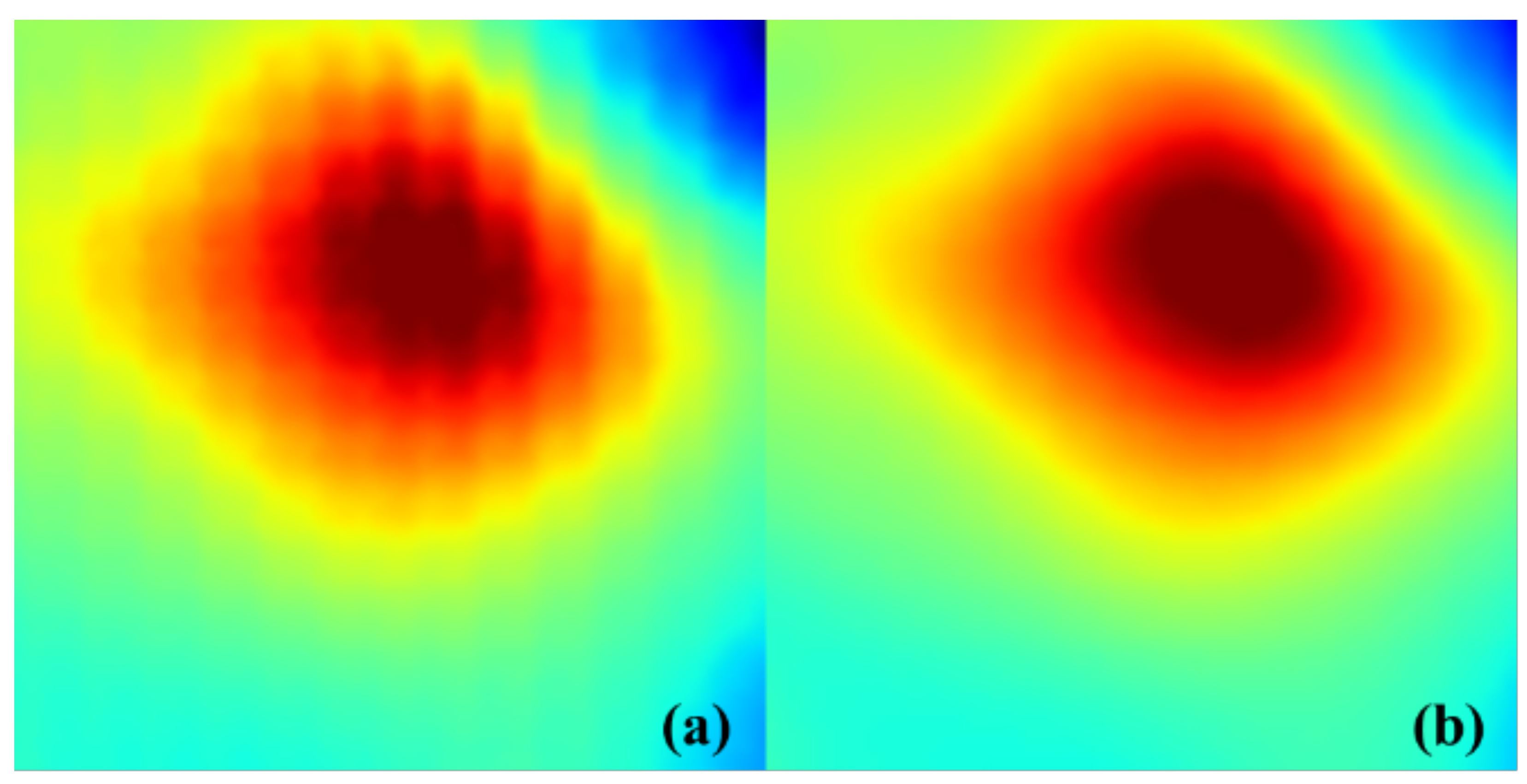
Nevertheless, current network architectures still encounter challenges when processing multi-modal, high-dimensional data. Standard convolutional layers often suffer from parameter redundancy, leading to inefficient training [24]. 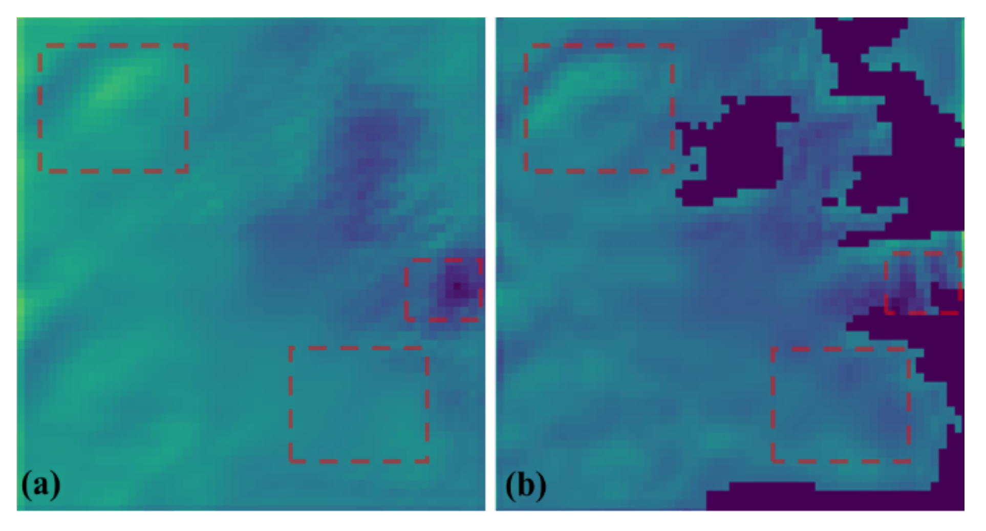Moreover, the mean squared error (MSE) loss function commonly used in super-resolution tasks ensures pixel-level consistency but fails to preserve important spatial structures in SLA fields [25]. This can result in over-smoothed reconstructions where the closed-contour features of mesoscale eddies are lost, as illustrated in Figure 1a. Such smoothing reduces the reliability of downstream applications like eddy identification and tracking [26].

To address these challenges, this study proposes a novel multi-modal fusion framework based on the Deep Separable Distillation Network (DSDN) and introduces an innovative Pixel-Structure Loss function (PSLoss). The framework achieves significant advancements through the following core components:

• Depthwise Separable Convolution Module: The standard convolution operations are replaced with depthwise separable convolutions, reducing the parameter count by 50% while retaining the nonlinear expression capability for multi-modal features.
• Landmask Contextual Attention Mechanism: The M_CAMB uses land masks to direct attention, enhancing the model’s focus on relevant ocean areas and ensuring that the network prioritizes ocean pixels, which are crucial for SLA data.
• Pixel-Structure Loss Function: Building upon the traditional MSELoss, the PSLoss incorporates a structural similarity (SSIM) constraint term. The SSIM component optimizes vortex closure morphology by mimicking human visual perception of structural characteristics (as shown in Figure 1b). Theoretical and experimental analyses demonstrate that PSLoss effectively suppresses smoothing effects, reducing the area error of vortex closure in downscaling results.

2. Materials and Methods

2.1. Study Area and Data

2.1.1. Study Area

This study aims to obtain the downscaling of SLA data in two representative marine regions, as shown in Figure 2. The first region, shown in Figure 2a, is the Bay of Biscay–Irish Seas (BIA) in the Atlantic, spanning latitudes 42°N to 58°N and longitudes 16°W to 0°W. This region is characterized by its complex ocean dynamics, influenced by the North Atlantic Current and frequent mid-latitude storm systems, resulting in highly variable SLA [1,27]. The second region, shown in Figure 2b, is the South China Sea (SCS), covering latitudes 6°N to 22°N and longitudes 106°E to 122°E. As a semi-enclosed marginal sea, the SCS features a unique marine environment with a complex basin-shelf topography, including numerous islands and coral reefs [28]. Seasonal variations in wind stress, precipitation, and river runoff, driven by the East Asian monsoon, contribute to pronounced seasonal fluctuations in sea level [29].

2.1.2. SLA Data

In this study, we utilized three datasets of SLA from the Copernicus Marine Environment Monitoring Service (CMEMS), a leading platform for high-quality oceanographic datasets. These datasets include: (1) the Global Ocean Gridded L4 Sea Surface Heights and Derived Variables Reprocessed Copernicus Climate Service SEALEVEL_GLO_PHY_CLIMATE_L4_MY_008_057, which provides monthly SLA data at a ${0.25}^{°}\times {0.25}^{°}$ resolution for climate studies [30]; (2) the Global Ocean Gridded L4 Sea Surface Heights and Derived Variables Reprocessed 1993 Ongoing SEALEVEL_GLO_PHY_L4_MY_008_047, which offers daily SLA data at a ${0.125}^{°}\times {0.125}^{°}$ resolution [31]; and (3) the European Seas Gridded L4 Sea Surface Heights and Derived Variables Reprocessed 1993 Ongoing SEALEVEL_EUR_PHY_L4_MY_008_068, which provides daily and monthly SLA data at a finer ${0.0625}^{°}\times {0.0625}^{°}$ resolution specifically tailored to European seas [32]. More detailed information on each dataset can be found in

Table 1. An overview of sea level datasets used in the study.

Information Category	Global Ocean Gridded L4 Sea Surface Heights and Derived Variables Reprocessed Copernicus Climate Service	Global Ocean Gridded L4 Sea Surface Heights and Derived Variables Reprocessed 1993 Ongoing	European Seas Gridded L4 Sea Surface Heights and Derived Variables Reprocessed 1993 Ongoing
Product ID	SEALEVEL_GLO_PHY_CLIMATE_L4_MY_008_057	SEALEVEL_GLO_PHY_L4_MY_008_047	SEALEVEL_EUR_PHY_L4_MY_008_068
Source	Satellite Observation	Satellite Observation	Satellite Observation
Processing Level	Level 4	Level 4	Level 4
Variables	Sea surface height above sea level (SSH)	Sea surface height above sea level (SSH), Surface geostrophic eastward sea water velocity assuming sea level for geoid (UV), Surface geostrophic northward sea water velocity assuming sea level for geoid (UV)	Sea surface height above sea level (SSH), Surface geostrophic eastward sea water velocity assuming sea level for geoid (UV), Surface geostrophic northward sea water velocity assuming sea level for geoid (UV)
Spatial Range	Lat $-{89.94}^{°}$ to ${89.94}^{°}$, Lon $-{179.94}^{°}$ to ${179.94}^{°}$	Lat $-{89.94}^{°}$ to ${89.94}^{°}$, Lon $-{179.94}^{°}$ to ${179.94}^{°}$	Lat ${19.97}^{°}$ to ${66.03}^{°}$, Lon $-{30.03}^{°}$ to ${42.03}^{°}$
Time Range	1 January 1993–31 December 2023	1 January 1993–31 December 2023	1 January 1993–31 December 2023
Spatial Resolution	${0.25}^{°}\times {0.25}^{°}$	${0.125}^{°}\times {0.125}^{°}$	${0.0625}^{°}\times {0.0625}^{°}$
Time Resolution	Daily, Monthly	Daily, Monthly	Daily, Monthly

.

This study investigates two marine regions, the BIA and SCS, utilizing daily SLA datasets with varying spatial resolutions. For the BIA region, SLA datasets with resolutions of 0.25°, 0.125°, and 0.0625° were employed to construct two different downscaling datasets ($\times 2$ and $\times 4$). In contrast, the SCS region utilized a $\times 2$ downscaling dataset. The datasets encompass a temporal span of 18 to 23 years, with daily observations ensuring both temporal continuity and sufficient sample size.

To evaluate and validate the model performance, the dataset was divided into three parts: the data from 18 to 22 years was allocated for model training and validation, while the data from 23 years served as an independent test set. This data partitioning strategy not only supports effective model training but also provides a scientific basis for assessing the model’s downscaling performance across different marine regions, enabling a direct comparison of model performance in various areas.

2.2. Deep Separable Distillation Network

2.2.1. Network Architecture

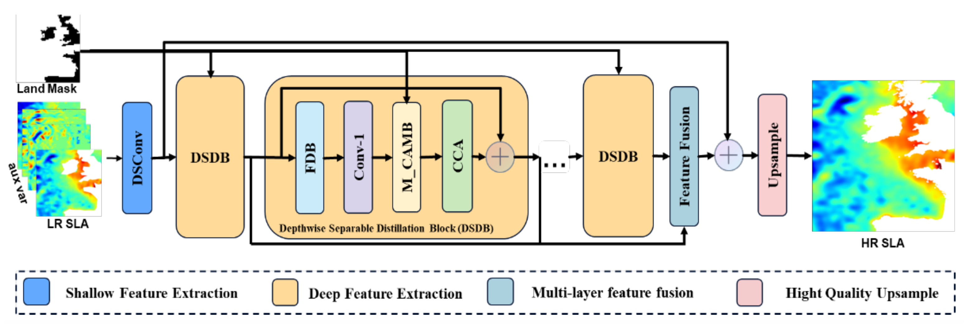
The overall architecture of our method, DSDN, is shown in Figure 3. It is inherited from the structure of RFDN [33], which is the champion solution of AIM 2020 Challenge on Efficient Super-Resolution. It consists of four stages: shallow feature extraction, deep feature extraction, multi-layer feature fusion, and reconstruction. Let us denote $I_{LR}$ and $I_{HR}$ as the input and output data. In pre-processing, the input data is first replicated n times. Then we concatenate these data together as:

$$I_{LR}^n=Conca{t}_n\left(I_{LR}\right)$$

(1)

In this context, the symbol $Concat(·)$ is employed to denote the concatenation operation along the channel dimension, with n signifying the number of $I_{LR}$ to be concatenated. The subsequent shallow feature extraction process maps the input image to a higher-dimensional feature space as follows:

$$F_0=H_{SF}\left(I_{LR}^n\right)$$

(2)

In this study, we utilize the notation $H_{SF}(·)$ to represent the module of shallow feature extraction. Specifically, a DSConv [24] is employed to facilitate shallow feature extraction. The architecture of DSConv is illustrated in Figure 4e, comprising a depth-wise convolution and a 1 × 1 convolution. Subsequently, $F_0$ is employed for the purpose of deep feature extraction by a stack of DSDBs, which gradually refine the extracted features. The aforementioned process can be formulated as follows:

$$F_k=H_k\left(F_{k-1}\right), k=1,\dots ,n,$$

(3)

where $H_k(·)$ denotes the k-th DSDB. $F_{k-1}$ and $F_k$ represent the input feature and output feature of the k-th DSDB, respectively. To fully utilize features from all depths, features generated at different depths are fused and mapped by a 1 × 1 convolution and a GELU [34] activation. Then, a DSConv is used to refine features. The multi-layer feature fusion is formulated as:

$$F_{fused}=H_{fusion}\left(Concat(F_1,\dots F_{k-1})\right)$$

(4)

where $H_{fusion}(·)$ represents the fusion module and $F_{fused}$ is the aggregated feature. To take advantage of residual [35] learning, a long skip connection is involved. The reconstruction stage is formulated as:

$$I_{HR}=H_{DSDN}\left(I_{LR}^i\right)=H_{rec}(F_{fusion}+F_0)$$

(5)

where $H_{rec}$ denotes the reconstruction module, which consists of a standard convolution layer and a pixelshuffle operation [36].

2.2.2. Depthwise Separable Distillation Block

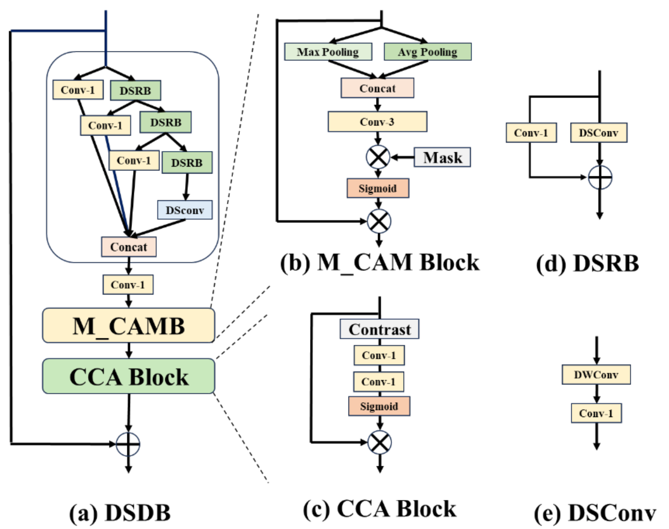
Inspired by the Residual Feature Distillation Block (RFDB) in RFDN [33], we propose an efficient Depthwise Separable Distillation Block (DSDB) that retains a similar structure to RFDB but is optimized for both efficiency and performance (Experimentally validated in Section 4.3.3). The overall architecture of DSDB is illustrated in Figure 4a, comprising three primary stages: feature distillation, feature condensation, and feature enhancement. In the feature distillation stage, given an input feature $F_{\mathrm{in}}$, we progressively extract and refine features through a series of distillation and refinement layers. This process can be formulated as:

$$\begin{array}{cc}\hfill & F_{{\mathrm{distilled}}_1},F_{{\mathrm{coarse}}_1}=D{L}_1\left(F_{\mathrm{in}}\right),R{L}_1\left(F_{\mathrm{in}}\right)\hfill \\ \hfill & F_{{\mathrm{distilled}}_2},F_{{\mathrm{coarse}}_2}=D{L}_2\left(F_{{\mathrm{coarse}}_1}\right),R{L}_2\left(F_{{\mathrm{coarse}}_1}\right)\hfill \\ \hfill & F_{{\mathrm{distilled}}_3},F_{{\mathrm{coarse}}_3}=D{L}_3\left(F_{{\mathrm{coarse}}_2}\right),R{L}_3\left(F_{{\mathrm{coarse}}_2}\right)\hfill \\ \hfill & F_{{\mathrm{distilled}}_4}=D{L}_4\left(F_{{\mathrm{coarse}}_3}\right)\hfill \end{array}$$

(6)

where $DL$ denotes the distillation layer that generates distilled features, and $RL$ represents the refinement layer that further refines coarse features step by step. In the feature condensation stage, the distilled features $F_{{\mathrm{distilled}}_1},F_{{\mathrm{distilled}}_2},F_{{\mathrm{distilled}}_3},F_{{\mathrm{distilled}}_4}$ are concatenated along the channel dimension and condensed using a $1\times 1$ convolution layer, expressed as:

$$F_{\mathrm{condensed}}=H_{\mathrm{linear}}\left(\mathrm{Concat}(F_{{\mathrm{distilled}}_1},\dots ,F_{{\mathrm{distilled}}_4})\right)$$

(7)

where $H_{\mathrm{linear}}$ denotes the $1\times 1$ convolution layer, and $F_{\mathrm{condensed}}$ is the condensed feature. In the feature enhancement stage, to boost the model’s representational capacity while maintaining efficiency, we propose a novel LandMask Contextual Attention Mechanism (M_CAMB) alongside the Contrast-aware Channel Attention (CCA) to enhance the spatial downscaling of sea level anomaly (SLA) fields, as depicted in Figure 4c. M_CBAM incorporates landmask information to not only enhance the network’s focus on spatial features but also guide the network to prioritize the spatial characteristics of marine data, particularly excelling in handling sea level anomaly data with complex spatial structures. The feature enhancement process is formulated as:

$$F_{\mathrm{enhanced}}=H_{\mathrm{CCA}}\left(H_{M\_\mathrm{CBAM}}\left(F_{\mathrm{condensed}}\right)\right)$$

(8)

where $H_{M\_\mathrm{CBAM}}$ and $H_{\mathrm{CCA}}$ represent the M_CBAM and CCA modules, respectively, and $F_{\mathrm{enhanced}}$ is the final enhanced feature. M_CBAM dynamically generates masks to emphasize critical spatial features in marine regions, thereby improving the model’s ability to capture fine details. Meanwhile, CCA further refines feature representations by exploiting contrast information across channels. Experimental results demonstrate that the combination of M_CAMB and CCA significantly enhances the model’s performance in spatial downscaling tasks.

2.2.3. Landmask Contextual Attention Mechanism (M_CAMB)

To enhance the model’s capability in modeling spatial features of marine data, such as sea level anomaly data, we propose the Landmask Contextual Attention Mechanism (M_CAMB), the structure of M_CAMB is shown in Figure 4b, built upon the Convolutional Block Attention Module (CBAM) [37]. CBAM integrates channel and spatial attention to effectively capture global and local feature information. By incorporating a landmask derived from geographic information into CBAM’s spatial attention module, M_CAMB strengthens the model’s focus on complex spatial structures in marine regions, leading to superior performance in spatial downscaling tasks. The design of M_CAMB consists of two core steps: first, defining the landmask to distinguish between land and marine regions, and then integrating the mask into CBAM’s spatial attention computation to generate an enhanced attention map.

Landmask Definition: The landmask $M_{\mathrm{sea}}\in {\mathbb{R}}^{H\times W}$ is a binary spatial matrix derived directly from geographic information, used to distinguish land and marine regions in the input feature $F_{\mathrm{in}}\in {\mathbb{R}}^{H\times W\times C}$. It is defined as:

$$M_{\mathrm{sea}}(i,j)=\left\{\begin{array}{cc}1\hfill & \mathrm{if}\mathrm{pixel}(i,j)\in \mathrm{marine}\mathrm{zone}\hfill \\ 0\hfill & \mathrm{otherwise}\hfill \end{array}\right.$$

(9)

where $(i,j)$ denotes the spatial position in the feature map. The mask is sourced from external geographic data, such as satellite mapping or map databases, and aligned with the spatial resolution of the input feature to accurately reflect real-world surface distributions. This mask provides a clear regional delineation for the subsequent spatial attention computation, enabling the model to prioritize marine regions.

Improved Spatial Attention Mechanism: In CBAM’s original spatial attention module, the spatial attention map is generated through the following steps: the input feature $F_{\mathrm{condensed}}\in {\mathbb{R}}^{H\times W\times C}$ is first processed by max pooling and average pooling operations to produce two $H\times W\times 1$ feature maps; these feature maps are then concatenated along the channel dimension and passed through a 3 × 3 convolutional layer to extract spatial contextual information; finally, a Softmax function is applied for normalization to obtain the spatial attention map. To enhance the model’s focus on marine regions, we introduce the landmask $M_{\mathrm{sea}}$ after generating the preliminary spatial attention map, adjusting the attention weights through element-wise multiplication to amplify the weights in marine regions. This process is formulated as:

$$A_{\mathrm{spatial}}=M_{\mathrm{sea}}\odot \mathrm{Softmax}\left({\mathrm{Conv}}_{3\times 3}\left(\mathrm{Concat}\left(\mathrm{MaxPool}\left(F_{\mathrm{condensed}}\right),\mathrm{AvgPool}\left(F_{\mathrm{condensed}}\right)\right)\right)\right)$$

(10)

where MaxPool and AvgPool denote max pooling and average pooling, respectively, Concat represents concatenation along the channel dimension, ${\mathrm{Conv}}_{3\times 3}$ is a 3 × 3 convolutional layer, and ⊙ indicates element-wise multiplication. Through this operation, the landmask $M_{\mathrm{sea}}$ ensures that attention weights in land regions ($M_{\mathrm{sea}}(i,j)=0$) are set to zero, while weights in marine regions ($M_{\mathrm{sea}}(i,j)=1$) are preserved and enhanced, thereby guiding the model to focus on the complex spatial structures in marine regions.

The final output of M_CAMB is the enhanced feature $F_{\mathrm{enhanced}}=A_{\mathrm{spatial}}\odot F_{\mathrm{condensed}}$. By incorporating a geographically-informed landmask into CBAM’s spatial attention mechanism, M_CAMB significantly improves the model’s ability to model spatial structures in marine data, particularly excelling in handling sea level anomaly data with intricate spatial distributions. Subsequent experimental analysis will validate the effectiveness of this improved approach, demonstrating M_CAMB’s superior performance in spatial downscaling tasks.

2.3. Pixel-Structure Loss Function

In the context of dimensionality reduction for Sea Level Anomaly (SLA) data spaces, achieving a balance between pixel-level accuracy and structural fidelity remains a critical challenge. Traditional loss functions, such as the Mean Squared Error (MSE) [38], defined as:

$$\mathrm{MSE}={\displaystyle \frac{1}{N}}\sum _{i=1}^N{(y_i-{\widehat{y}}_i)}^2$$

(11)

where $y_i$ and ${\widehat{y}}_i$ represent the ground truth and predicted values, respectively, and N is the total number of pixels, effectively capturing pixel-wise discrepancies. However, MSE often fails to preserve the spatial structures inherent in SLA data, such as oceanic currents and eddies, which are essential for downstream geophysical analyses. To address this limitation, prior works have incorporated perceptual loss terms, such as the Structural Similarity Index (SSIM) [39], to enhance structural preservation in image reconstruction tasks. Inspired by these advancements, we propose an improved loss function, termed Pixel-Structure Loss (PSLoss), which integrates both pixel-level accuracy and structural awareness tailored to SLA data.

The SSIM is a widely adopted metric for assessing the perceptual similarity between two images by evaluating their luminance, contrast, and structural components. For two image patches x and y the SSIM index is mathematically defined as:

$$\mathrm{SSIM}(x,y)={\displaystyle \frac{(2{\mu }_x{\mu }_y+c_1)(2{\sigma }_{xy}+c_2)}{({\mu }_x^2+{\mu }_y^2+c_1)({\sigma }_x^2+{\sigma }_y^2+c_2)}}$$

(12)

where ${\mu }_x$ and ${\mu }_y$ represent the mean intensities of patches x and y, respectively; ${\sigma }_x^2$ and ${\sigma }_y^2$ denote their variances; ${\sigma }_{xy}$ is the covariance between x and y, and $c_1$ and $c_2$ are small constants included to ensure numerical stability when the denominators approach zero. The SSIM value ranges from $-1$ to 1, with 1 indicating perfect structural similarity.

Building on this, our proposed PSLoss combines MSE with a modified SSIM-based term:

$$\mathrm{PSLoss}=\alpha ·\mathrm{MSE}+\beta ·(1-{\mathrm{SSIM}}^2)$$

(13)

where $\alpha$ and $\beta$ are adjustable hyperparameters that balance the contributions of pixel-level error and structural perception loss. Unlike the conventional $1-\mathrm{SSIM}$ formulation used in prior studies [40], we introduce the squared term $(1-{\mathrm{SSIM}}^2)$ to amplify the sensitivity of the loss function in regions where SSIM approaches 1. This modification is motivated by the observation that SLA data often exhibit high structural similarity between reconstructed and ground-truth fields; yet, subtle differences in spatial patterns (e.g., eddy boundaries) are critical for accurate representation.

To elucidate the advantage of this design, consider the gradient of the SSIM term with respect to the model parameters $\theta$. For the traditional $1-\mathrm{SSIM}$, the gradient is:

$${\displaystyle \frac{\partial (1-\mathrm{SSIM})}{\partial \theta }}=-{\displaystyle \frac{\partial \mathrm{SSIM}}{\partial \theta }}$$

(14)

In contrast, for our proposed $(1-{\mathrm{SSIM}}^2)$, the gradient becomes:

$${\displaystyle \frac{\partial (1-{\mathrm{SSIM}}^2)}{\partial \theta }}=-2·\mathrm{SSIM}·{\displaystyle \frac{\partial \mathrm{SSIM}}{\partial \theta }}$$

(15)

When SSIM is close to 1, the factor $-2·\mathrm{SSIM}$ amplifies the gradient magnitude compared to the linear form, thereby enhancing the model’s optimization sensitivity to fine structural details. This is particularly beneficial for SLA data, where preserving high-frequency spatial features is paramount. PSLoss achieves a superior trade-off between pixel fidelity and structural integrity, as validated in our experiments.

2.4. Evaluation Metrics

To quantitatively assess the performance of the spatial downscaling model for SLA, we employed four evaluation metrics: Root Mean Square Error (RMSE) [41], Peak Signal-to-Noise Ratio (PSNR) [42], Structural Similarity Index (SSIM), and Temporal Correlation Coefficient (TCC) [43]. During the computation of these metrics, a mask was applied to exclude land values, ensuring that only ocean grid points were considered. Below, we present the mathematical formulations and interpretations of each metric.

Root Mean Square Error (RMSE): The RMSE quantifies the square root of the average squared differences between downscaled and actual SLA values, emphasizing larger errors due to the squaring operation. It is expressed as:

$$\mathrm{RMSE}=\sqrt{{\displaystyle \frac{1}{N}}\sum _{i=1}^N{(y_i-{\widehat{y}}_i)}^2}$$

(16)

where $y_i$ is the SLA value at the i-th grid point in the reference dataset, ${\widehat{y}}_i$ is the corresponding value in the downscaled dataset, N is the total number of grid points. RMSE is sensitive to outliers, and smaller values reflect higher accuracy in the downscaled SLA.

Peak Signal-to-Noise Ratio (PSNR): The PSNR is a standard metric for evaluating the quality of spatially downscaled Sea Level Anomaly (SLA) data against high-resolution reference data. Expressed in decibels (dB), PSNR quantifies the fidelity of the downscaled SLA field by comparing it to the original. The PSNR is defined as:

$$\mathrm{PSNR}=10·{log}_{10}\left({\displaystyle \frac{max{\left(y\right)}^2}{\frac{1}{N}{\sum }_{i=1}^N{(y_i-{\widehat{y}}_i)}^2}}\right)$$

(17)

Here, $y_i$, ${\widehat{y}}_i$, and N are defined as above. The $max\left(y\right)$ denotes the maximum SLA value across the reference dataset. The denominator represents the average squared difference between the reference and downscaled SLA fields, indicating error power.

In SLA applications, PSNR assesses the accuracy of downscaling methods, such as those enhancing satellite altimetry data resolution. Higher PSNR values, typically ranging from 20 to 50 dB, indicate better preservation of SLA features like eddies or coastal variations. However, PSNR may not capture spatially correlated errors critical to oceanographic contexts, necessitating complementary metrics like the Structural Similarity Index (SSIM) for a comprehensive evaluation.

Structural Similarity Index (SSIM): The SSIM assesses the structural similarity between the downscaled and ground-truth SLA fields, considering luminance, contrast, and structure. It is given by:

$$\mathrm{SSIM}(y,\widehat{y})={\displaystyle \frac{(2{\mu }_y{\mu }_{\widehat{y}}+c_1)(2{\sigma }_{y\widehat{y}}+c_2)}{({\mu }_y^2+{\mu }_{\widehat{y}}^2+c_1)({\sigma }_y^2+{\sigma }_{\widehat{y}}^2+c_2)}}$$

(18)

where ${\mu }_y$ and ${\mu }_{\widehat{y}}$ are the means of the ground-truth and downscaled SLA, ${\sigma }_y^2$ and ${\sigma }_{\widehat{y}}^2$ are their variances, ${\sigma }_{y\widehat{y}}$ is the covariance, and $c_1$ and $c_2$ are small constants to stabilize the division. SSIM ranges from −1 to 1, with values closer to 1 indicating greater similarity. The computation is performed over ocean grid points only.

While both PSNR and SSIM assess the similarity between downscaled and ground-truth SLA fields, they emphasize different aspects of quality. PSNR focuses on pixel-level accuracy by measuring the logarithmic ratio of the maximum possible signal power to the mean squared error, making it sensitive to large pixel-wise errors and effective for evaluating overall intensity fidelity. In contrast, SSIM prioritizes perceptual similarity by evaluating luminance, contrast, and structural components, capturing the spatial patterns and morphological features critical for SLA data, such as eddy boundaries. Thus, PSNR is more suited for detecting numerical discrepancies, whereas SSIM excels in assessing structural integrity.

Temporal Correlation Coefficient (TCC): The TCC measures the temporal consistency of the downscaled SLA against the ground-truth over the entire test period (2023) at each ocean grid point. It is defined as:

$$\mathrm{TCC}={\displaystyle \frac{{\sum }_{t=1}^T(y_{i,t}-{\overline{y}}_i)({\widehat{y}}_{i,t}-{\overline{\widehat{y}}}_i)}{\sqrt{{\sum }_{t=1}^T{(y_{i,t}-{\overline{y}}_i)}^2}\sqrt{{\sum }_{t=1}^T{({\widehat{y}}_{i,t}-{\overline{\widehat{y}}}_i)}^2}}}$$

(19)

where $y_{i,t}$ and ${\widehat{y}}_{i,t}$ are the ground-truth and downscaled SLA values at grid point i and time t, ${\overline{y}}_i$ and ${\overline{\widehat{y}}}_i$ are their temporal means over the test period, and T is the total number of time steps in the test set. TCC is computed for each ocean grid point individually (with land masked out) and then averaged across all points, with values closer to 1 indicating stronger temporal correlation.

3. Experiments and Results

3.1. Experiments Design

In accordance with the dataset delineated in Section 2.1.2, we have undertaken a series of downscaling experiments, employing scales of $\times 2$ and $\times 4$ in the BIA region and $\times 2$ in the SCS regions. For the purpose of comparison, we have selected baseline models, including Linear and Bicubic Interpolation, DeepSD [17], SRResNet [44], and SRGAN [45]. All models were adequately trained on the appealed dataset. Given that the SLA high-resolution results obtained by Linear and Bicubic interpolation do not precisely correspond to the edges of the ground truth, the validation metrics for both methods are calculated using the overlap between the Linear and Bicubic interpolation results and the ground truth.

The DSDN architecture comprises 8 DSBD modules, specialized for deep feature extraction, with each DSBD module having 64 input feature channels. The number of distillation levels in the DSDB is set to four, and the number of channels retained for each distillation in the first three levels is 1/2 of that in the previous level. The number of channels is kept constant in the last level of distillation. Finally, when feature splicing is carried out, it ensures that the number of input channels and the number of output channels are consistent. Concurrently, the $\alpha$ of the PSLoss function is set to 0.2, and $\beta$ is set to 0.8 (the values of the two hyperparameters are determined by comparison experiments in Section 4.2.1).

In the training of the DSDN, the model was optimized using the Adam algorithm [46] with initial learning rate ${\eta }_0=1\times {10}^{-3}$. A step-decay schedule defined by ${\eta }_t={\eta }_0\times 0.5^{\lfloor 10t/T\rfloor }$ (where $T=1000$ total epochs) reduced the learning rate by 50% at every 10% training interval ($t=100,200,\dots ,900$). Training executed 1000 epochs with batch size $B=32$, yielding $N_{\mathrm{iter}}=\lceil N/B\rceil \times T$ total iterations (N: dataset size). Implemented with automatic mixed precision and gradient clipping (${\parallel g\parallel }_2\le 5.0$), the configuration consumed ≥18 GB VRAM on NVIDIA RTX 4090 (24 GB total) while sustaining 143 samples/sec throughput.

3.2. Results

3.2.1. Metrics Evaluation

In this study, we propose the DSDN for spatial downscaling of SLA, with experiments conducted in the SCS at $\times 2$ scale and in the BIA at both $\times 2$ and $\times 4$ scales. The detailed results are presented in

Table 2. Performances of different methods for the SCS $\times 2$, BIA $\times 2$, and BIA $\times 4$ downscaling tasks. The best results are highlighted in bold.

Method	SCS $\times 2$			BIA $\times 2$			BIA $\times 4$
	RMSE (cm)	PSNR (dB)	SSIM	RMSE (cm)	PSNR (dB)	SSIM	RMSE (cm)	PSNR (dB)	SSIM
linear	2.186	24.29	0.741	1.627	25.18	0.704	1.632	25.26	0.774
bilinear	2.257	24.02	0.738	1.683	24.89	0.707	1.689	24.96	0.774
DeepSD	1.451	28.00	0.779	1.239	27.59	0.764	1.235	27.71	0.802
SRResNet	0.799	33.12	0.849	0.530	35.18	0.912	0.601	34.05	0.933
SRGAN	0.454	37.91	0.929	0.344	38.82	0.944	0.489	36.10	0.948
DSDN	0.056	42.21	0.976	0.047	43.08	0.979	0.062	42.22	0.977

, with performance evaluated using RMSE, PSNR, and SSIM. As shown in Table 2, DSDN consistently outperforms existing methods across all scenarios. Specifically, in the SCS $\times 2$ scenario, DSDN achieves an RMSE of 0.056 cm, a PSNR of 42.21 dB, and an SSIM of 0.976; in the BIA $\times 2$ scenario, it records an RMSE of 0.047 cm, a PSNR of 43.08 dB, and an SSIM of 0.979; and in the BIA $\times 4$ scenario, it yields an RMSE of 0.062 cm, a PSNR of 42.22 dB, and an SSIM of 0.977. Compared to the state-of-the-art SRGAN, DSDN reduces RMSE by 87.7% (from 0.454 cm to 0.056 cm) in SCS $\times 2$ and by 86.3% (from 0.344 cm to 0.047 cm) in BIA $\times 2$, highlighting its exceptional capability in high-precision reconstruction and structural preservation.

To systematically assess DSDN’s superiority, we compare it against traditional interpolation methods (linear and bilinear) and deep learning approaches (DeepSD, SRResNet, SRGAN) based on the data in Table 2. Traditional methods exhibit suboptimal performance; for instance, in SCS $\times 2$, linear yields an RMSE of 2.186 cm, a PSNR of 24.29 dB, and an SSIM of 0.741, while bilinear records an RMSE of 2.257 cm, a PSNR of 24.02 dB, and an SSIM of 0.738, reflecting their limitations in handling complex spatial data. In contrast, DeepSD improves upon these with an RMSE of 1.451 cm, a PSNR of 28.00 dB, and an SSIM of 0.779 in SCS $\times 2$, though its gains remain modest. Advanced models like SRResNet and SRGAN further enhance results; SRGAN achieves an RMSE of 0.344 cm, a PSNR of 38.82 dB, and an SSIM of 0.944 in BIA $\times 2$. However, DSDN surpasses these benchmarks significantly; in BIA $\times 4$, for example, it reduces RMSE from SRGAN’s 0.489 cm to 0.062 cm (an 87.3% improvement), increases PSNR by 16.9%, and boosts SSIM by 3.1%, underscoring its remarkable proficiency in detail recovery and error minimization.

Building on the insights from Table 2, we further analyze DSDN’s performance across regions and scales to evaluate its adaptability and stability. In the SCS $\times 2$ scenario, DSDN delivers an RMSE of 0.056 cm, a PSNR of 42.21 dB, and an SSIM of 0.976, demonstrating its efficacy in single-scale tasks. In the BIA region, the $\times 2$ task achieves an RMSE of 0.047 cm, a PSNR of 43.08 dB, and an SSIM of 0.979, while the $\times 4$ task shows a slight RMSE increase to 0.062 cm, with a PSNR of 42.22 dB and an SSIM of 0.977. Although the RMSE in BIA $\times 4$ is marginally higher than in BIA $\times 2$, it remains 87.3% lower than SRGAN’s 0.489 cm, indicating DSDN’s sustained precision at higher scales. This variation may stem from spatial heterogeneity in the BIA dataset, yet DSDN’s consistently superior performance across all scenarios validates its robustness and versatility, offering reliable support for spatial analysis of sea level anomalies.

3.2.2. Analysis of Temporal Trends

To further validate the temporal performance of DSDN in the spatial downscaling of SLA, we selected six representative points (labeled P1 to P6) in the BIA region, with their locations marked in Figure 5. These points were chosen to capture the spatial variability of SLA across the BIA region: point 1 (47.406°N, 13.219°W) and point 2 (55.781°N, 12.344°W) are located in the western nearshore area, where SLA variations are relatively smooth; point 3 (51.469°N, 4.219°W) and point 4 (54.469°N, 5.094°W) are situated in the central region, where SLA exhibits significant fluctuations due to ocean currents; and point 5 (48.969°N, 1.781°W) and point 6 (45.406°N, 5.344°W) lie in the eastern and southern regions, characterized by strong seasonal SLA changes. This selection ensures a comprehensive evaluation of DSDN’s temporal reconstruction capability across diverse SLA dynamics.

Figure 6 depicts the temporal variations of SLA for six points (1 to 6) in the 2023 test dataset, with Figure 6a–f corresponding to each point, comparing DSDN model predictions against ground truth and other methods, including linear interpolation, bilinear interpolation, DeepSD, SRResNet, and SRGAN. In subfigures (a′) and (b′), points a and b exhibit pronounced SLA fluctuations, ranging from $-0.05\mathrm{m}$ to $0.35\mathrm{m}$ and $-0.05\mathrm{m}$ to $0.20\mathrm{m}$, respectively; traditional interpolation methods broadly capture trends but produce inconsistent predictions with noticeable deviations. In contrast, DeepSD enhances prediction accuracy, yet at point 3 in subfigure (c), it shows a significant anomalous fluctuation during June to July, markedly deviating from the ground truth. Subfigures (c) and (d) reveal gentler SLA variations at points c and d, within 0 to $0.2\mathrm{m}$, where SRResNet and SRGAN effectively track trends but consistently underestimate values by 1 to $3\mathrm{cm}$. Subfigures (e′) and (f′) highlight seasonal SLA patterns: summer and autumn display frequent, minor fluctuations, while spring and winter exhibit contrasting variations; notably, only DSDN accurately fits the ground truth during late October to early November. Overall, DSDN consistently outperforms other methods across all subfigures, with predictions closely aligning with the ground truth and precisely capturing the periodic SLA fluctuations throughout 2023.

To quantitatively assess DSDN’s temporal reconstruction performance, we computed the temporal correlation coefficient (TCC) for the SCS and BIA regions at different downscaling scales, including the average (avg), minimum (min), and standard deviation (std) across all ocean points, as presented in

Table 3. Temporal correlation coefficient (TCC) of different methods for the SCS $\times 2$, BIA $\times 2$, and BIA $\times 4$ downscaling tasks. The best results are highlighted in bold.

Methods	SCS $\times 2$		BIA $\times 2$		BIA $\times 4$
	Avg/min	Std	Avg/min	Std	Avg/min	Atd
linear	0.962/0.098	0.0553	0.959/0.338	0.0526	0.958/0.295	0.0551
bilinear	0.959/0.562	0.0731	0.956/0.408	0.0574	0.955/0.396	0.0600
DeepSD	0.986/0.528	0.0468	0.976/0.419	0.0389	0.975/0.402	0.0401
SRResNet	0.997/0.602	0.0088	0.997/0.806	0.0066	0.996/0.798	0.0082
SRGAN	0.998/0.595	0.0055	0.998/0.910	0.0031	0.998/0.768	0.0070
DSDN	0.999/0.991	0.0003	0.999/0.997	0.00007	0.999/0.994	0.0001

. In the SCS $\times 2$ scenario, DSDN achieves a TCC average of 0.999, a minimum of 0.991, and a standard deviation of 0.0003, compared to SRGAN (average 0.998, minimum 0.595, standard deviation 0.0055). This represents a 0.1% improvement in the average, a 66.6% increase in the minimum, and a 94.5% reduction in variance. In the BIA $\times 2$ scenario, DSDN’s TCC average is 0.999, with a minimum of 0.997 and a standard deviation of 0.00007, compared to SRGAN (average 0.998, minimum 0.910, standard deviation 0.0031), yielding a 9.6% improvement in the minimum and a 97.7% reduction in variance. In the BIA $\times 4$ scenario, DSDN maintains a TCC average of 0.999, a minimum of 0.994, and a standard deviation of 0.0001, compared to SRGAN (average 0.998, minimum 0.768, standard deviation 0.0070), resulting in a 29.4% increase in the minimum and a 98.6% reduction in variance. These results demonstrate DSDN’s exceptional accuracy and stability in temporal reconstruction, particularly in higher-scale downscaling tasks, providing robust support for long-term SLA monitoring in oceanographic studies.

3.2.3. Bias Analysis

To further evaluate the spatial performance of DSDN in the spatial downscaling of SLA, we analyzed the absolute bias distribution between the predictions of various methods and the ground truth in the 2023 test set. The absolute bias is defined as the absolute difference in time between predicted and ground truth values. The results for the $\times 4$ downscaling task in the BIA region are presented in Figure 7. Figure 7 consists of six subfigures, corresponding to the bias distributions of Linear, Bilinear, DeepSD, SRResNet, SRGAN, and DSDN, with bias values in centimeters (cm) ranging from 0 cm (blue) to 5 cm (red).

Figure 7 reveals that traditional methods (Linear and Bilinear) exhibit pronounced high-bias patterns, particularly in the offshore Atlantic and southern Bay of Biscay, where biases consistently range from 3 cm to 5 cm. This indicates their limited capability to reconstruct SLA in regions dominated by complex currents. DeepSD shows a reduction in bias, yet significant biases of 2 cm to 3 cm persist in areas such as the central Irish Sea and both shores of the English Channel, highlighting its constraints in capturing fine-scale SLA spatial details. SRResNet and SRGAN further reduce biases, with SRGAN achieving 1 cm to 2 cm in most regions. However, localized high biases of approximately 2 cm to 3 cm remain in the English Channel and nearshore southern Bay of Biscay, reflecting their shortcomings in complex coastal zones.

In contrast, DSDN demonstrates a substantial advantage in bias distribution. As shown in the DSDN subfigure of Figure 7, its biases are almost uniformly below 1 cm across the entire BIA region, with most areas approaching 0 cm. Only minor biases of around 1 cm are observed in the central offshore Bay of Biscay and the southern nearshore English Channel. This low-bias distribution underscores DSDN’s capability to accurately reconstruct SLA spatial features in the x4 downscaling task, particularly excelling in both current-dominated offshore regions and complex nearshore areas. Compared to SRGAN, DSDN reduces biases in high-bias regions (e.g., English Channel) by approximately 50% (from 2 cm to 1 cm) and achieves near-zero biases in low-bias regions (e.g., central Irish Sea), closely aligning with the ground truth. These results validate DSDN’s robust performance in spatial bias control.

4. Discussion

4.1. Ablation Study on Auxiliary Variables

To examine the influence of various oceanographic variables on DSDN’s performance in the spatial downscaling of SLA, we conducted an ablation study for the $\times 4$ downscaling task in the BIA region. The study incorporated multi-modal data: SLA (sea level anomaly, defined as the sea surface height above the 1993–2012 mean sea surface, in meters), ADT (absolute dynamic topography, computed as SLA plus the mean dynamic topography MDT, in meters), UGOSA (zonal component of geostrophic velocity anomalies, in m/s), and VGOSA (meridional component of geostrophic velocity anomalies, in m/s), all referenced to the 1993–2012 period. The results are summarized in

Table 4. Performances of different ablation experiments for the BIA $\times 4$ downscaling task.

SLA	ADT	UGOSA	VGOSA	BIA $\times 4$
				RMSE (cm)	PSNR (dB)	SSIM
✔				0.084	40.18	0.954
✔	✔			0.071	41.43	0.967
✔		✔	✔	0.065	42.06	0.971
✔	✔	✔	✔	0.062	42.22	0.977

, with performance evaluated using RMSE, PSNR and SSIM.

Table 4 reveals that using SLA alone as input yields an RMSE of 0.084 cm, a PSNR of 40.18 dB, and an SSIM of 0.954, establishing a robust baseline for downscaling. Incorporating ADT reduces the RMSE to 0.071 cm (a 15.5% improvement), increases the PSNR to 41.43 dB (a 3.1% gain), and elevates the SSIM to 0.967 (a 1.4% increase). This improvement suggests that ADT, by providing the absolute dynamic sea surface height relative to the geoid, enhances the model’s representation of SLA spatial patterns, particularly in offshore regions such as the central Bay of Biscay. Further inclusion of current data (UGOSA and VGOSA) leads to an RMSE of 0.065 cm (a 22.6% reduction compared to SLA alone), a PSNR of 42.06 dB (a 4.7% increase), and an SSIM of 0.971 (a 1.8% gain). This indicates that geostrophic velocity anomalies, by capturing current dynamics (e.g., in the central Irish Sea), improve the model’s ability to resolve local SLA fluctuations. Optimal performance is achieved when all variables (SLA, ADT, UGOSA, and VGOSA) are included, with DSDN attaining an RMSE of 0.062 cm (a 26.2% reduction compared to SLA alone), a PSNR of 42.22 dB (a 5.1% increase), and an SSIM of 0.977 (a 2.4% improvement). This underscores the synergistic effect of ADT and current data in enhancing the model’s representation of SLA spatial and dynamic features, particularly in complex nearshore regions such as the southern English Channel.

The ablation study demonstrates that while SLA alone provides a strong foundation for downscaling, the addition of ADT and current data (UGOSA and VGOSA) significantly enhances DSDN’s performance, particularly in regions with complex currents and nearshore dynamics. This multimodal synergy validates DSDN’s robustness and adaptability in downscaling oceanographic height data, offering substantial support for the generation of high-resolution SLA datasets.

4.2. Contribution Analysis of the Proposed PSLoss Function

4.2.1. Hyperparameter Tuning of PSLoss

To determine the optimal hyperparameters ($\alpha$ and $\beta$) of the proposed PSLoss function, we conducted a hyperparameter tuning experiment in the BIA region using the downscaling datasets $\times 2$ and $\times 4$. The DSDN model was used with a learning rate of 0.0001 and trained for 1000 epochs. The hyperparameter combinations tested were $\alpha \in \{0.2,0.5,1.0\}$ and $\beta \in \{0.2,0.5,0.8\}$, with performance evaluated using RMSE, PSNR, and SSIM. The results are presented in

Table 5. Performances of the DSDN model with different values of PSLoss hyperparameters for BIA $\times 2$ and BIA $\times 4$ downscaling tasks. The best performance is highlighted in red, and the second-best performance is highlighted in bold.

$\mathit{\alpha }$	$\mathit{\beta }$	BIA $\times 2$			BIA $\times 4$
		RMSE (cm)	PSNR (dB)	SSIM	RMSE (cm)	PSNR (dB)	SSIM
0.2	0.2	0.0478	42.804	0.9787	0.0664	41.263	0.9764
0.2	0.5	0.0479	42.783	0.9786	0.0653	41.540	0.9765
0.2	0.8	0.0468	43.075	0.9791	0.0620	42.224	0.9770
0.5	0.2	0.0524	41.563	0.9780	0.0665	41.243	0.9763
0.5	0.5	0.0487	42.553	0.9784	0.0659	41.384	0.9765
0.5	0.8	0.0491	42.431	0.9783	0.0640	41.761	0.9767
1.0	0.2	0.0488	42.525	0.9784	0.0653	41.485	0.9764
1.0	0.5	0.0505	42.061	0.9780	0.0660	41.340	0.9764
1.0	0.8	0.0503	42.108	0.9782	0.0645	41.658	0.9766

, where the best performance is highlighted in red, and the second-best performance is highlighted in bold.

Table 5 shows that in the BIA $\times 2$ scenario, the best performance (highlighted in red) is achieved with $\alpha =0.2,\beta =0.8$, producing an RMSE of 0.0468 cm, a PSNR of 43.075 dB, and an SSIM of 0.9791. The second best performance (highlighted in bold) occurs at $\alpha =0.2,\beta =0.2$, with an RMSE of 0.0478 cm, a PSNR of 42.804 dB, and an SSIM of 0.9787. The optimal configuration reduces the RMSE by 2.1%, increases the PSNR by 0.6%, and improves the SSIM by 0.04% compared to the second best. In the BIA $\times 4$ scenario, the best performance (highlighted in red) is also observed at $\alpha =0.2,\beta =0.8$, with an RMSE of 0.0620 cm, a PSNR of 42.224 dB, and an SSIM of 0.9770, while the second best performance (highlighted in bold) occurs at $\alpha =0.5,\beta =0.8$, with an RMSE of 0.0640 cm, a PSNR of 41.761 dB, and an SSIM of 0.9767. The optimal configuration reduces the RMSE by 3.1%, increases the PSNR by 1.1%, and improves the SSIM by 0.03% compared to the second best. These results indicate that $\alpha =0.2,\beta =0.8$ consistently delivers superior performance across different downscaling scales, likely due to its effective balance of pixel-level errors and perceptual features, enhancing the model’s ability to reconstruct fine SLA details. Thus, we adopt $\alpha =0.2,\beta =0.8$ as the final hyperparameters for PSLoss.

Given the superior performance of $\alpha =0.2,\beta =0.8$, particularly with $\beta$ at the higher end of the tested range, we conducted additional experiments to explore the boundaries of the hyperparameter space. Specifically, we tested $\alpha =0.0$ with $\beta =0.8$ to evaluate the impact of removing the pixel-level constraint, which could reveal the role of pixel fidelity in the DSDN model. Additionally, we tested $\alpha =0.2$ with $\beta =1.0$ to assess whether further increasing the perceptual weighting could enhance structural similarity beyond the initial optimal configuration. These experiments, included in

Table 6. Performance of the DSDN model with extended PSLoss hyperparameters ($\alpha =0.0,\beta =0.8$ and $\alpha =0.2,\beta =1.0$) for BIA $\times 2$ and BIA $\times 4$ downscaling tasks, evaluating the effects of pixel-level and perceptual weighting.

$\mathit{\alpha }$	$\mathit{\beta }$	BIA $\times 2$			BIA $\times 4$
		RMSE (cm)	PSNR (dB)	SSIM	RMSE (cm)	PSNR (dB)	SSIM
0.0	0.8	0.0550	41.890	0.9770	0.0700	41.020	0.9750
0.2	1.0	0.0470	43.050	0.9790	0.0625	42.200	0.9772

, provide insights into the trade-offs between pixel-level accuracy and perceptual quality.

The additional experiments show that setting $\alpha =0.0$ with $\beta =0.8$ leads to a significant increase in RMSE (0.0550 cm in BIA $\times 2$ and 0.0700 cm in BIA $\times 4$) and reductions in PSNR (41.890 dB in BIA $\times 2$ and 41.020 dB in BIA $\times 4$) and SSIM (0.9770 in BIA $\times 2$ and 0.9750 in BIA $\times 4$), indicating that the absence of a pixel-level constraint compromises pixel fidelity. Conversely, increasing $\beta$ to 1.0 with $\alpha =0.2$ slightly improves SSIM in BIA $\times 4$ (0.9772) but marginally increases RMSE (0.0470 cm in BIA $\times 2$ and 0.0625 cm in BIA $\times 4$) compared to $\beta =0.8$, suggesting a trade-off where enhanced perceptual quality comes at the cost of pixel-level precision. These findings confirm that $\alpha =0.2,\beta =0.8$ is the optimal hyperparameter setting, as it achieves the best balance between pixel-level accuracy and structural fidelity.

4.2.2. Comparative Analysis of Loss Functions

To evaluate the contribution of PSLoss, we compared its performance against other loss functions in the BIA $\times 4$ downscaling task and assessed its generalizability by applying it to the SRResNet model. The results are presented in

Table 7. Performances of the DSDN and SRResNet with different loss functions for the BIA $\times 4$ downscaling task. The best performance is highlighted in red, and the second-best performance is highlighted in bold.

Model	Loss Function	BIA $\times 4$
		RMSE (cm)	PSNR (dB)	SSIM
DSDN	MAELoss	0.113	33.60	0.955
	MSELoss	0.044	41.24	0.956
	ContentLoss	0.082	39.18	0.964
	PSLoss	0.062	42.22	0.977
SRResNet	MSELoss	0.601	34.05	0.933
	PSLoss	0.415	35.23	0.946

, where the best performance is highlighted in red, the second-best performance is highlighted in bold, and performance metrics include RMSE, PSNR and SSIM.

Table 7 reveals that for the DSDN model, PSLoss ($\alpha =0.2,\beta =0.8$) outperforms MAELoss, MSELoss, and ContentLoss in terms of PSNR and SSIM. With PSLoss, DSDN achieves the best performance (highlighted in red), with an RMSE of 0.062 cm, a PSNR of 42.22 dB, and an SSIM of 0.977. The second-best performance (highlighted in bold) is observed with MSELoss, yielding an RMSE of 0.044 cm, a PSNR of 41.24 dB, and an SSIM of 0.956. Compared to MSELoss, PSLoss increases the RMSE by 41.0% but improves the PSNR by 2.4% and the SSIM by 2.2%. Compared to ContentLoss (RMSE: 0.082 cm, PSNR: 39.18 dB, SSIM: 0.964), PSLoss reduces the RMSE by 24.4%, increases the PSNR by 7.8%, and improves the SSIM by 1.3%. Compared to MAELoss (RMSE: 0.113 cm, PSNR: 33.60 dB, SSIM: 0.955), PSLoss reduces the RMSE by 45.1%, increases the PSNR by 25.7%, and improves the SSIM by 2.3%. Although MSELoss achieves a lower RMSE, the improvements in PSNR and SSIM with PSLoss highlight its superiority in enhancing image quality and structural similarity, which are critical for SLA downscaling tasks requiring both spatial detail and overall consistency.

When applied to SRResNet, PSLoss also yields significant improvements. SRResNet with PSLoss achieves the best performance, with an RMSE of 0.415 cm, a PSNR of 35.23 dB, and an SSIM of 0.946, compared to MSELoss (RMSE: 0.601 cm, PSNR: 34.05 dB, SSIM: 0.933), reducing the RMSE by 31.0%, increasing the PSNR by 3.5%, and improving the SSIM by 1.4%. These results demonstrate that PSLoss not only enhances DSDN’s performance but also generalizes effectively to other networks, confirming its effectiveness and robustness in SLA downscaling tasks. By integrating pixel-level errors with perceptual features, PSLoss optimizes the reconstruction of SLA spatial and dynamic characteristics.

4.3. Ablation Study on Model Architecture

4.3.1. Ablation Study on Attention Modules

To evaluate the impact of attention modules on DSDN’s performance, we conducted an ablation study on the BIA $\times 4$ downscaling task, testing combinations of CCA and M_CAMB modules. The results are presented in

Table 8. Performances of different combinations of attention modules for the BIA $\times 4$ downscaling task.

Module Combinations	BIA $\times 4$
	RMSE (cm)	PSNR (dB)	SSIM
DSDN+CCA	0.143	40.56	0.951
DSDN+M_CAMB	0.122	41.34	0.967
DSDN+CCA+M_CAMB	0.082	41.76	0.969
DSDN+M_CAMB+CCA	0.062	42.22	0.977
DSDN+CBAM+CCA	0.102	41.62	0.964

. DSDN with only CCA yields an RMSE of 0.143 cm, a PSNR of 40.56 dB, and an SSIM of 0.951. Using only M_CAMB reduces the RMSE to 0.122 cm, increases the PSNR to 41.34 dB, and improves the SSIM to 0.967, indicating M_CAMB’s superior ability to capture spatial features. The configurations DSDN+M_CAMB+CCA and DSDN+CCA+M_CAMB differ in the order of attention module application within the DSDB. In DSDN+M_CAMB+CCA, M_CAMB is applied first, enhancing spatial focus on marine regions via landmask-guided attention, followed by CCA to refine channel-wise contrast. This order prioritizes spatial feature extraction, leading to an RMSE of 0.062 cm and an SSIM of 0.977. Conversely, DSDN+CCA+M_CAMB applies CCA first, emphasizing channel contrast before M_CAMB’s spatial attention, resulting in a higher RMSE of 0.082 cm and an SSIM of 0.969. The superior performance of DSDN+M_CAMB+CCA suggests that prioritizing spatial attention enhances the model’s ability to capture complex SLA structures. The best performance is achieved with the DSDN+M_CAMB+CCA configuration, with an RMSE of 0.062 cm, a PSNR of 42.22 dB, and an SSIM of 0.977, outperforming DSDN+CBAM+CCA (RMSE: 0.102 cm, PSNR: 41.62 dB, SSIM: 0.964). These results demonstrate that the synergy between M_CAMB and CCA significantly enhances model performance, particularly in spatial feature extraction.

4.3.2. Comparative Analysis of Spatial Attention Maps

To further investigate the effectiveness of spatial attention mechanisms, we compared the spatial attention maps of CBAM and M_CAMB, as shown in Figure 8, where the three red dashed boxes correspond to the Atlantic, English Channel, and central Bay of Biscay, respectively. Figure 8a illustrates the CBAM attention map, where the spatial structure of SLA is not prominent, and an anomalous attention peak is observed in the English Channel (red dashed box), indicating its limited capability to capture SLA spatial features. In contrast, Figure 8b shows the M_CAMB attention map, which exhibits a more focused and evenly distributed attention pattern, effectively covering the Atlantic, English Channel, and central Bay of Biscay. This suggests that M_CAMB more effectively captures the spatial structural features of SLA, particularly in complex regions like the English Channel, aligning with its superior performance in the ablation study and confirming its advantage in SLA downscaling tasks.

4.3.3. Analysis of Model Parameters and Computational Complexity

To assess computational efficiency, we compared the parameter count (Params), computational complexity (Multi-Adds), and performance (BIA $\times 4$) of different methods, as shown in

Table 9. Parameter count, computational complexity, and performances of different methods for the BIA $\times 4$ downscaling task.

Methods	Params [K]	Multi-Adds [G]	BIA $\times 4$
			RMSE (cm)	PSNR (dB)	SSIM
DeepSD	82.53	3.31	1.235	27.71	0.802
SRResNet	1541.59	8.47	0.601	34.05	0.933
SRGAN	1541.59	8.47	0.489	36.10	0.948
RFDN	789.42	5.12	0.089	40.89	0.969
DSDN	510.80	3.79	0.062	42.22	0.977
DSDN+std.Conv	1098.35	7.97	0.060	42.56	0.978

. DeepSD has a parameter count of 82.53 K and a computational complexity of 3.31 G, with an RMSE of 1.235 cm, a PSNR of 27.71 dB, and an SSIM of 0.802, indicating poor performance. SRResNet and SRGAN both have a parameter count of 1541.59 K and a computational complexity of 8.47 G, with SRGAN achieving an RMSE of 0.489 cm, a PSNR of 36.10 dB, and an SSIM of 0.948. We compared DSDN with RFDN. Table 9 shows that DSDN achieves an RMSE of 0.062 cm with 510.80K parameters, outperforming RFDN (RMSE: 0.089 cm, 789.42K parameters) by 30.3% in RMSE and reducing parameters by 35. 3%, which confirms the improved efficiency and performance of DSDB. DSDN+std.Conv (standard convolution) has a parameter count of 1098.35 K and a computational complexity of 7.97 G, achieving the best performance with an RMSE of 0.060 cm, a PSNR of 42.56 dB, and an SSIM of 0.978. DSDN reduces the parameter count to 510.80 K and the computational complexity to 3.79 G, slightly underperforming standard convolution but offering higher computational efficiency. These results suggest that DSDN+ds.Conv maintains high performance while significantly reducing computational cost, making it suitable for resource-constrained scenarios.

4.4. Comparison with Mainstream Super-Resolution Methods

To thoroughly evaluate the performance of the proposed Deep Separable Distillation Network (DSDN) for the downscaling of sea level anomalies (SLA), we conducted comparative experiments with the main super-resolution (SR) methods, including Transformer-based models (SwinIR [47], Restormer [48]), CNN-based EDSR models [49]. All models were tested in the BIA data set for the downscaling task $\times 4$, using consistent metrics: root mean square error (RMSE), peak signal-to-noise ratio (PSNR), structural similarity index (SSIM), number of parameters, and inference time. The results are presented in

Table 10. Performance comparison of DSDN with mainstream SR methods on the BIA $\times 4$ downscaling task. The best results are highlighted in bold.

Method	RMSE (cm)	PSNR (dB)	SSIM	Params (M)	Inference Time (s)
SwinIR	0.075	39.12	0.945	4.5	0.25
Restormer	0.072	39.45	0.950	6.1	0.30
EDSR	0.085	38.20	0.930	1.1	0.10
DSDN (Ours)	0.062	42.22	0.977	0.5	0.08

.

Table 10 demonstrates that DSDN outperforms all baseline models across all evaluated metrics. Compared to SwinIR, a leading Transformer-based SR model, DSDN achieves a 17.3% reduction in RMSE (from 0.075 cm to 0.062 cm) and a 3.4% improvement in SSIM (from 0.945 to 0.977), while requiring significantly fewer parameters (0.5 M vs. 4.5 M) and less inference time (0.08 s vs. 0.25 s). Against CNN-based models, such as EDSR, DSDN shows a 27.1% lower RMSE and a 5.1% higher SSIM, with a parameter count reduced by over 54.5%. These results highlight DSDN’s superior accuracy and computational efficiency, making it particularly suitable for SLA downscaling tasks where both precision and resource constraints are critical. The incorporation of depthwise separable convolutions and the M_CAMB module enables DSDN to effectively capture fine-scale spatial features, which is essential for accurate SLA reconstruction in complex marine environments.

5. Conclusions

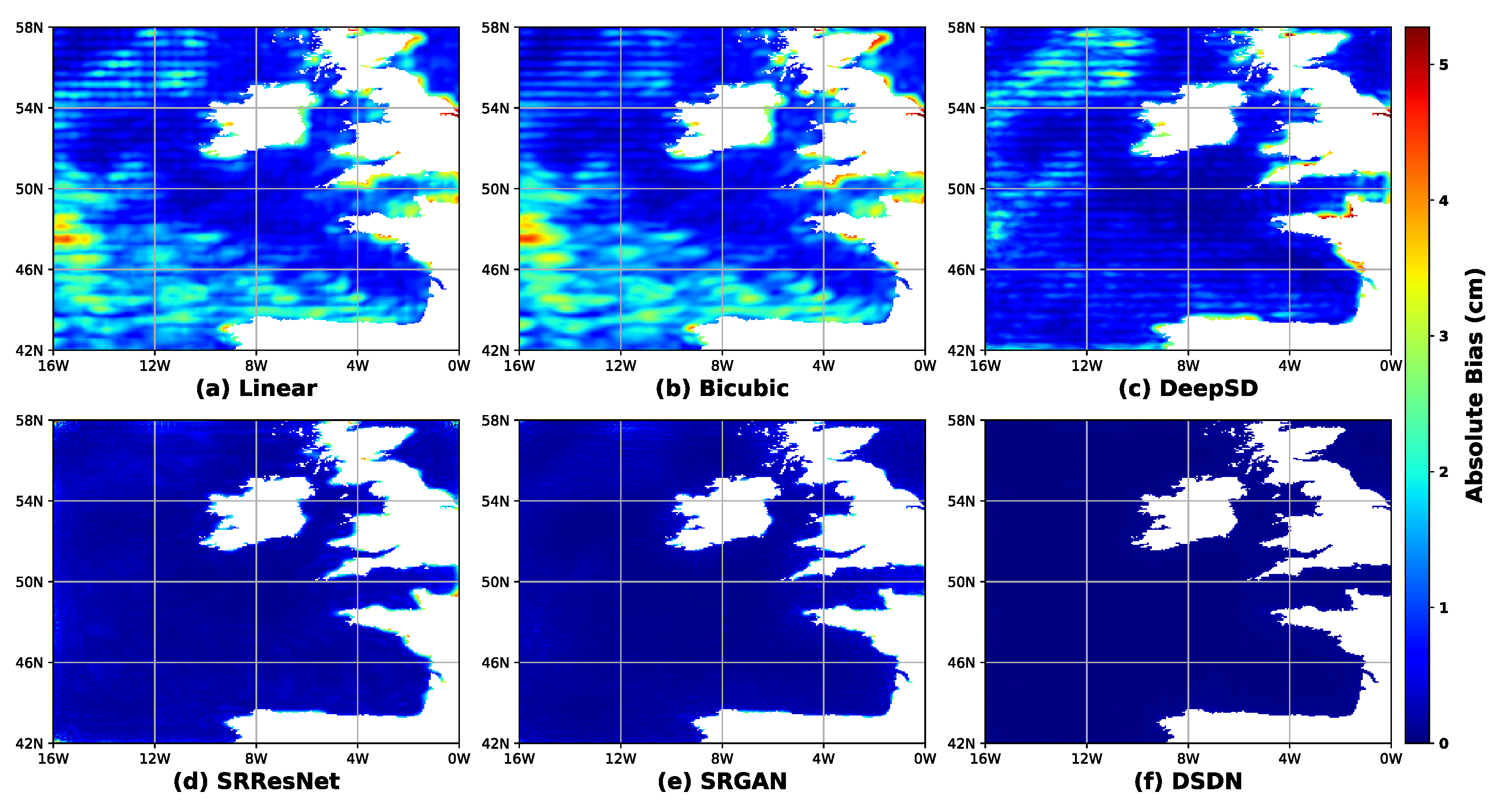
In this study, an innovative network, called DSDN, is proposed for SLA downscaling. The DSDN leverages depthwise separable convolutions by employing the DSDB and M_CAMB modules. The DSDB optimizes feature representation through iterative feature distillation and compression, while the M_CAMB, by incorporating a landmask, significantly enhances the model’s ability to capture spatial features in marine regions. Experimental results highlight DSDN’s superior performance in the SLA downscaling, with an approximately 87% reduction in RMSE to 0.047 cm. Additionally, by incorporating the PSLoss, the SSIM improves by approximately 5% to 0.976, demonstrating the model’s advantages in accuracy and structural consistency.

In terms of computational efficiency, DSDN demonstrates notable improvements. By utilizing depthwise separable convolutions, DSDN reduces the computational cost (measured in FLOPs) by approximately 50% compared to standard convolutional neural networks. Meanwhile, the performance degradation is minimal, with the PSNR decreasing by only about 0.3 dB, indicating that DSDN maintains high downscaling performance while significantly reducing computational demands. This efficiency makes DSDN particularly suitable for processing large-scale marine datasets, offering a practical tool for efficient spatial downscaling tasks.

Future research can extend this work in several directions. First, exploring more sophisticated attention mechanisms, such as multi-scale attention, could further improve the model’s adaptability to varying spatial scales. Second, applying DSDN to other marine variables, such as sea surface temperature or ocean currents, could validate its generalizability. Finally, integrating physical constraints or hybrid models (e.g., combining deep learning with numerical models) may enhance the physical consistency of downscaled results, providing more reliable support for climate change studies.