
Comparison of Artificial Intelligence Algorithms and Remote Sensing for Modeling Pine Bark Beetle Susceptibility in Honduras

 ,
,  , , ,
, , ,  , and
, and 
Abstract

1. Introduction
2. Materials and Methods
2.1. Study Area
2.2. Databases
2.2.1. Training Samples
2.2.2. Remote Sensing Data or Environmental Covariates

| No | Covariate | Collection | Observation |
|---|---|---|---|
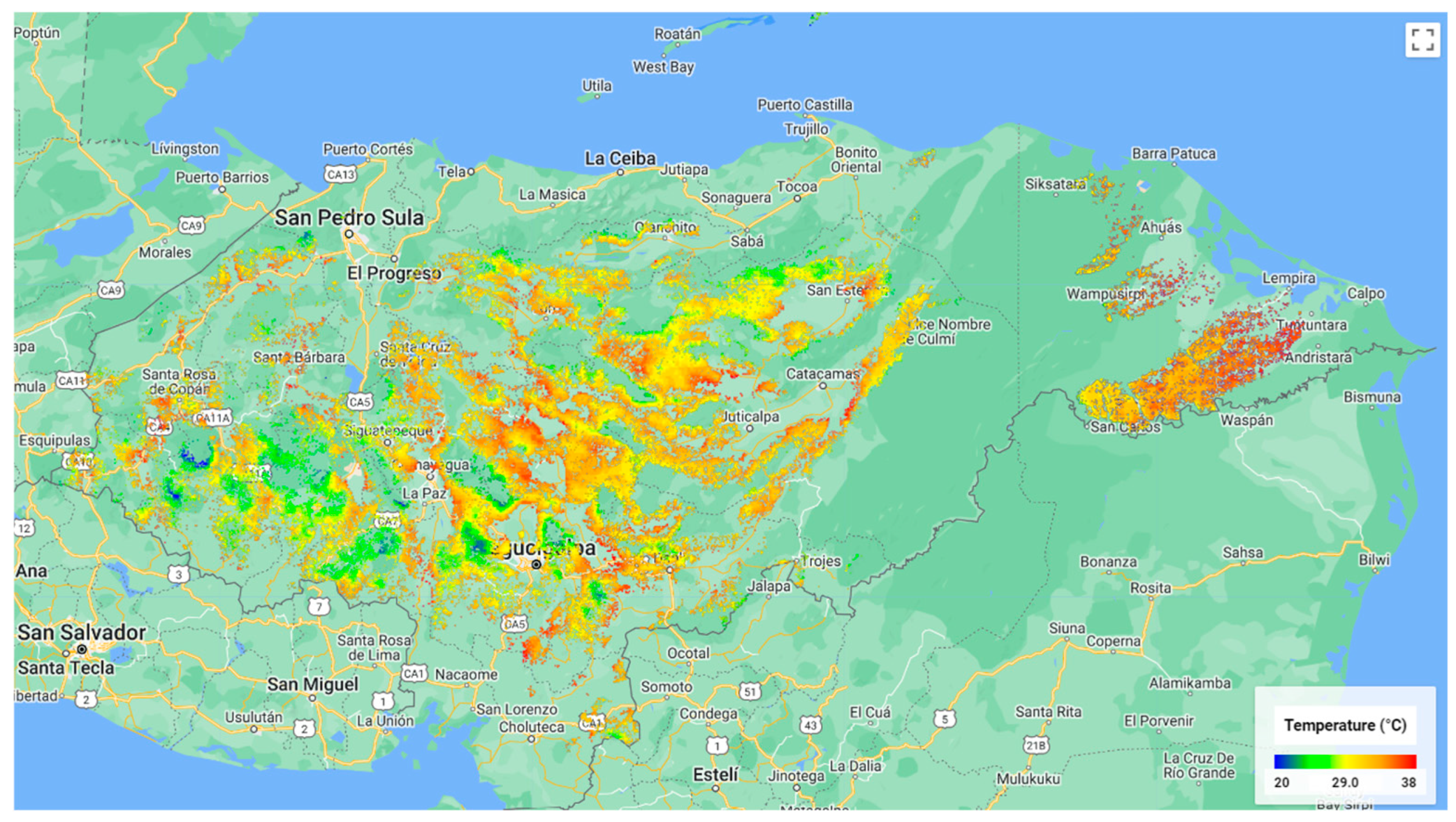
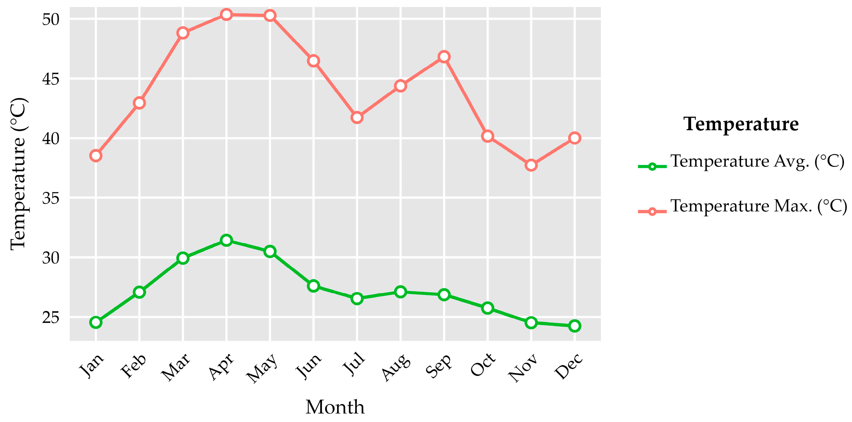
| 1 | Land surface temperature (LST) | MODIS/061/MOD11A2 | Provides 8-day averages of LST at 1 km resolution [83] |
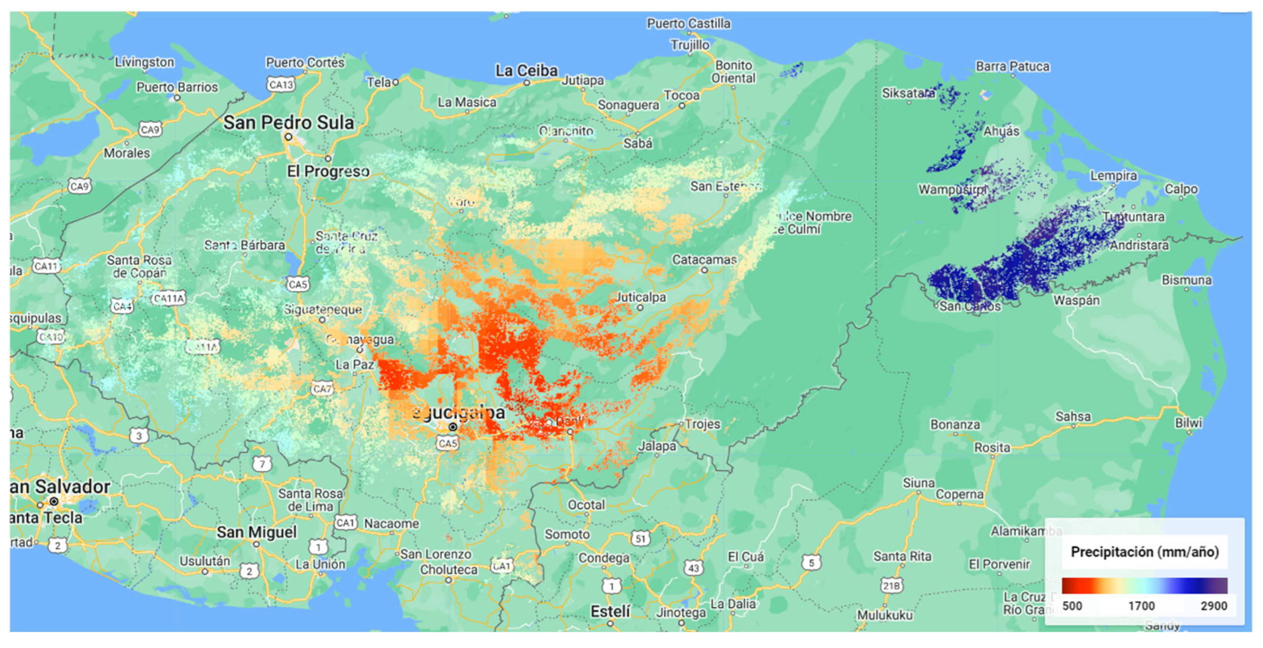
| 2 | Precipitation | UCSB-CHG/CHIRPS/DAILY | 0.05° resolution resampled to 1 km [84] |
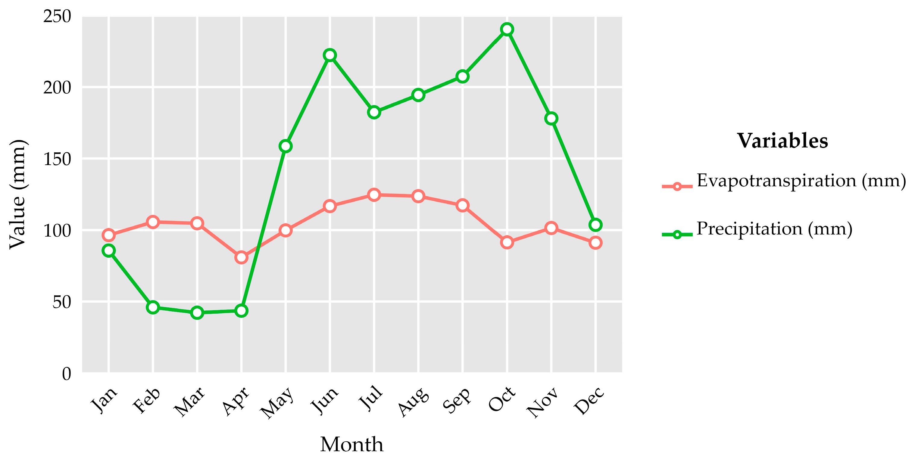
| 3 | Evapotranspiration | MODIS/NTSG/MOD16A2/105 | 8-day averages at 1 km resolution [85] |
| 4 | Normalized difference vegetation index (NDVI) | MODIS/061/MOD09A1 | MODIS multispectral images at 500 m resolution [86,87] |
| 5 | Normalized difference moisture index (NDMI) | MODIS/061/MOD09A1 | Same collection as NDVI [88] |
| 6 | Water deficit (WD) | Precipitation—evapotranspiration | 1 km resolution |
| 7 | Elevation (DEM) | WWF/HydroSHEDS/03CONDEM | Digital elevation model (DEM) with 100 m resolution [89] |
| 8 | Slope | WWF/HydroSHEDS/03CONDEM | Derived from elevation |
2.3. Remote Sensing Data Processing
2.4. Analysis of the Relationship Between the Covariates and Pest Occurrence
2.5. Artificial Intelligence or Machine Learning Algorithms Used
2.5.1. Random Forest
2.5.2. Gradient Boosting
2.5.3. Maximum Entropy
2.6. Selection and Optimization of Hyperparameters
2.7. Importance of Covariates
2.8. Spatial Susceptibility Modeling
2.9. Thematic Accuracy Estimation
3. Results
3.1. Relationship Between Environmental Covariates and the Pests
3.2. Best Hyperparameters
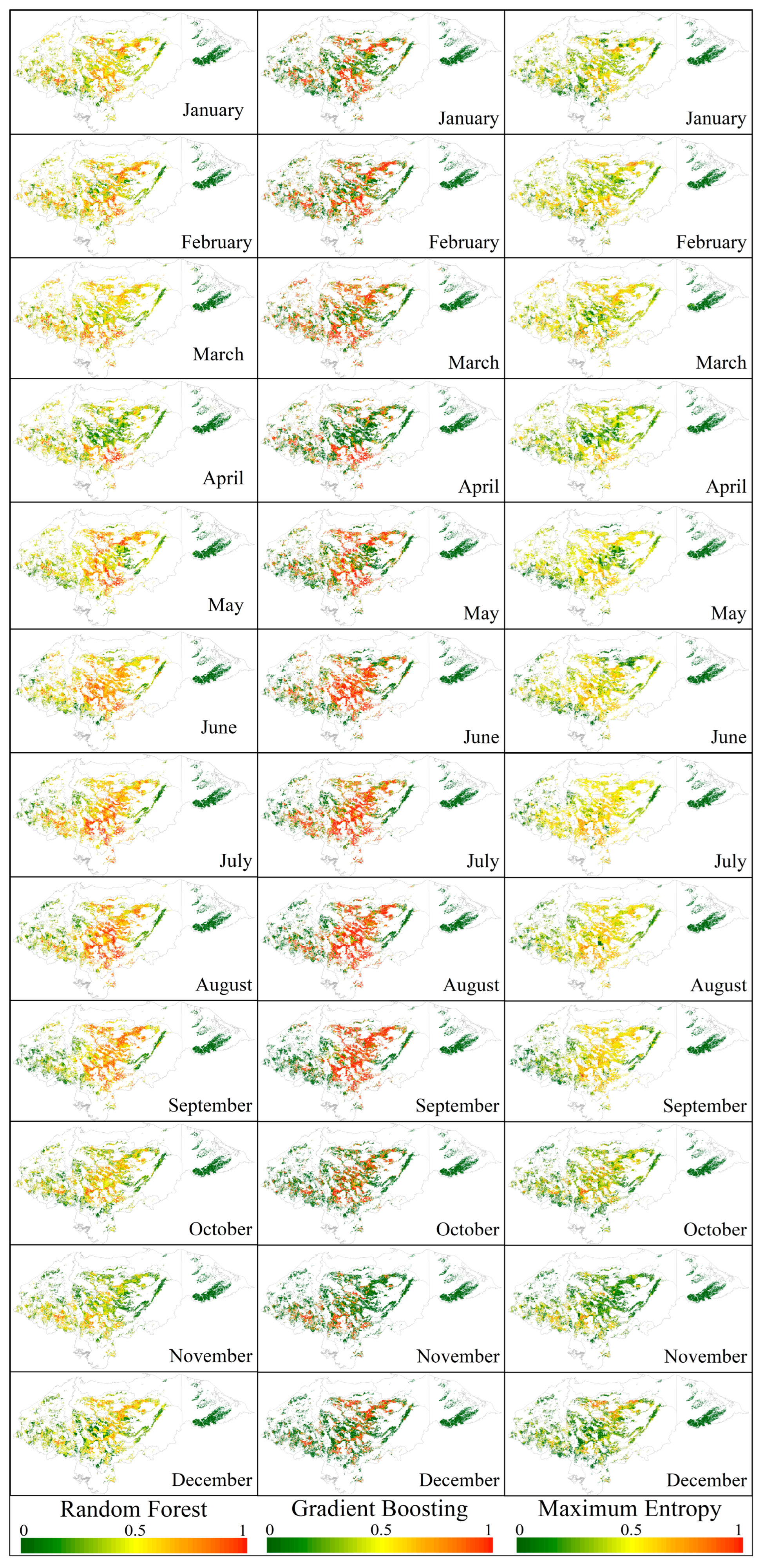
3.3. Spatial Susceptibility Models
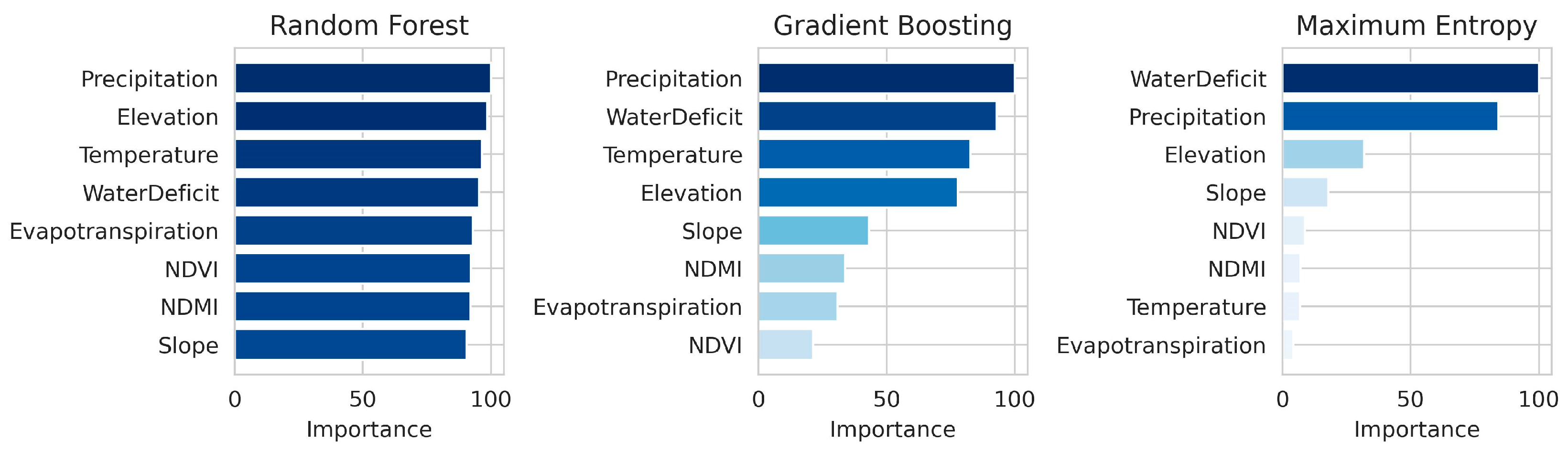
3.4. Importance of Environmental Covariates
3.5. Thematic Accuracy of the Models
4. Discussion
5. Conclusions
Author Contributions
Funding
Data Availability Statement
Acknowledgments
Conflicts of Interest
Appendix A

Appendix B
Appendix C
References
- Kolb, T.E.; Fettig, C.J.; Ayres, M.P.; Bentz, B.J.; Hicke, J.A.; Mathiasen, R.; Stewart, J.E.; Weed, A.S. Observed and Anticipated Impacts of Drought on Forest Insects and Diseases in the United States. For. Ecol. Manag. 2016, 380, 321–334. [Google Scholar] [CrossRef]
- Mezei, P.; Jakuš, R.; Pennerstorfer, J.; Havašová, M.; Škvarenina, J.; Ferenčík, J.; Slivinský, J.; Bičárová, S.; Bilčík, D.; Blaženec, M.; et al. Storms, Temperature Maxima and the Eurasian Spruce Bark Beetle Ips Typographus—An Infernal Trio in Norway Spruce Forests of the Central European High Tatra Mountains. Agric. For. Meteorol. 2017, 242, 85–95. [Google Scholar] [CrossRef]
- Subedi, B.; Poudel, A.; Aryal, S. The Impact of Climate Change on Insect Pest Biology and Ecology: Implications for Pest Management Strategies, Crop Production, and Food Security. J. Agric. Food Res. 2023, 14, 100733. [Google Scholar] [CrossRef]
- Sharma, H.C.; Prabhakar, C.S. Chapter 2—Impact of Climate Change on Pest Management and Food Security. In Integrated Pest Management; Abrol, D.P., Ed.; Academic Press: San Diego, CA, USA, 2014; pp. 23–36. ISBN 978-0-12-398529-3. [Google Scholar]
- Mukhtar, Y.; Shankar, U.; Wazir, Z.A. Prospects and Challenges of Emerging Insect Pest Problems Vis-à-Vis Climate Change. IJE 2023, 50, 1096–1103. [Google Scholar] [CrossRef]
- Panzavolta, T.; Bracalini, M.; Benigno, A.; Moricca, S. Alien Invasive Pathogens and Pests Harming Trees, Forests, and Plantations: Pathways, Global Consequences and Management. Forests 2021, 12, 1364. [Google Scholar] [CrossRef]
- Zenni, R.D.; Essl, F.; García-Berthou, E.; McDermott, S.M. The Economic Costs of Biological Invasions around the World. NeoBiota 2021, 67, 1–9. [Google Scholar] [CrossRef]
- Guégan, J.-F.; de Thoisy, B.; Gomez-Gallego, M.; Jactel, H. World Forests, Global Change, and Emerging Pests and Pathogens. Curr. Opin. Environ. Sustain. 2023, 61, 101266. [Google Scholar] [CrossRef]
- Krokene, P. Chapter 5—Conifer Defense and Resistance to Bark Beetles. In Bark Beetles; Vega, F.E., Hofstetter, R.W., Eds.; Academic Press: San Diego, CA, USA, 2015; pp. 177–207. ISBN 978-0-12-417156-5. [Google Scholar]
- Hlásny, T.; Krokene, P.; Liebhold, A.; Montagné-Huck, C.; Müller, J.; Qin, H.; Raffa, K.; Schelhaas, M.-J.; Seidl, R.; Svoboda, M.; et al. Living with Bark Beetles: Impacts, Outlook and Management Options; From Science to Policy; European Forest Institute: Joensuu, Finland, 2019. [Google Scholar]
- Fettig, C.J.; Asaro, C.; Nowak, J.T.; Dodds, K.J.; Gandhi, K.J.K.; Moan, J.E.; Robert, J. Trends in Bark Beetle Impacts in North America During a Period (2000–2020) of Rapid Environmental Change. J. For. 2022, 120, 693–713. [Google Scholar] [CrossRef]
- Hernandez, A.J.; Saborio, J.; Ramsey, R.D.; Rivera, S. Likelihood of Occurrence of Bark Beetle Attacks on Conifer Forests in Honduras under Normal and Climate Change Scenarios. Geocarto Int. 2012, 27, 581–592. [Google Scholar] [CrossRef]
- Valdez, M.C.; Chen, C.-F.; Lin, Y.-J.; Kuo, Y.-C.; Chen, Y.-Y.; Medina, D.; Diaz, K. Characterizing Spatial Patterns of Pine Bark Beetle Outbreaks during the Dry and Rainy Season’s in Honduras with the Aid of Geographic Information Systems and Remote Sensing Data. For. Ecol. Manag. 2020, 467, 118162. [Google Scholar] [CrossRef]
- Gómez, D.F.; Sathyapala, S.; Hulcr, J. Towards Sustainable Forest Management in Central America: Review of Southern Pine Beetle (Dendroctonus Frontalis Zimmermann) Outbreaks, Their Causes, and Solutions. Forests 2020, 11, 173. [Google Scholar] [CrossRef]
- Carías, A.; Barrios, J.; Espino, V.; Oqueli, R. Mitigation Strategies for the Attack of the Pine Bark Beetle in Honduras, Period 2014–2016. Cienc. Espac. 2018, 10, 198. [Google Scholar] [CrossRef]
- Padilla, M.A.M.; Zelaya, E.R.; López, T.D.G.; Núñez, F.A.P.; Hernández, B.E.S.; Godoy, M.E.E.; Chévez, G.S.P.; Reyes, D.R.M.; Posas, J.G.M.; Ulloa, A.A.L.; et al. Forest Reference Level Proposal of Honduras. 2020. Available online: https://redd.unfccc.int/media/nrf_honduras_2020_sumision_modificada.pdf (accessed on 24 November 2024).
- NOAA Annual 2015 Global Climate Report | National Centers for Environmental Information (NCEI). Available online: https://www.ncei.noaa.gov/access/monitoring/monthly-report/global/201513 (accessed on 22 October 2023).
- Navarro-Cerrillo, R.M.; Rodriguez-Vallejo, C.; Silveiro, E.; Hortal, A.; Palacios-Rodríguez, G.; Duque-Lazo, J.; Camarero, J.J. Cumulative Drought Stress Leads to a Loss of Growth Resilience and Explains Higher Mortality in Planted than in Naturally Regenerated Pinus Pinaster Stands. Forests 2018, 9, 358. [Google Scholar] [CrossRef]
- ICF. Anuario Estadístico Forestal de Honduras año 2017; ICF: Tegucigalpa, Honduras, 2017; p. 149. Available online: https://icf.gob.hn/wp-content/uploads/2023/10/Anuario-Forestal-2017.pdf (accessed on 24 November 2024).
- ICF. Informe del episodio del ataque del gorgojo descortezador del pino Dendroctonus frontalis en Honduras 2014–2017; ICF: Tegucigalpa, Honduras, 2017; p. 71. Available online: https://icf.gob.hn/wp-content/uploads/2024/05/Informe-Episodio-de-Plaga-2014-2017.pdf (accessed on 17 October 2024).
- Duarte, E.; Orellana, O.; Maradiaga, I.; Casco, F.; Fuentes, D.; Jimenez, A.; Emanuelli, P.; Milla, F. Mapa Forestal y de Cobertura de la Tierra de Honduras: Análisis de Cifras Nacionales; Programa REDD-CCAD/GIZ; ICF: Tegucigalpa, Honduras, 2014; Available online: https://www.researchgate.net/publication/305297234_Mapa_Forestal_y_de_Cobertura_de_la_Tierra_de_Honduras_Analisis_de_Cifras_Nacionales (accessed on 17 December 2024).
- Pratt, L.; Quijandría, G. Forestry Sector in Honduras: Sustainability Analysis; INCAE: La Garita, Costa Rica, 1997. [Google Scholar]
- López, D.Z.; Groothousen, C.; Núñez, J.P. Estimation of Pinus oocarpa Schiede Forest Yield Using Permanent Sampling Plots. Tatascán 2006, 18, 18. [Google Scholar]
- ICF. Forestry Statistical Yearbook of Honduras 2021; ICF: Tegucigalpa, Honduras, 2021; p. 131. [Google Scholar]
- Intralawan, A.; Wood, D.; Frankel, R.; Costanza, R.; Kubiszewski, I. Tradeoff Analysis between Electricity Generation and Ecosystem Services in the Lower Mekong Basin. Ecosyst. Serv. 2018, 30, 27–35. [Google Scholar] [CrossRef]
- Wang, L.; Zheng, H.; Wen, Z.; Liu, L.; Robinson, B.E.; Li, R.; Li, C.; Kong, L. Ecosystem Service Synergies/Trade-Offs Informing the Supply-Demand Match of Ecosystem Services: Framework and Application. Ecosyst. Serv. 2019, 37, 100939. [Google Scholar] [CrossRef]
- Kaura, M.; Arias, M.E.; Benjamin, J.A.; Oeurng, C.; Cochrane, T.A. Benefits of Forest Conservation on Riverine Sediment and Hydropower in the Tonle Sap Basin, Cambodia. Ecosyst. Serv. 2019, 39, 101003. [Google Scholar] [CrossRef]
- Wang, L.; Zheng, H.; Chen, Y.; Long, Y.; Chen, J.; Li, R.; Hu, X.; Ouyang, Z. Synergistic Management of Forest and Reservoir Infrastructure Improves Multistakeholders’ Benefits across the Forest-Water-Energy-Food Nexus. J. Clean. Prod. 2023, 422, 138575. [Google Scholar] [CrossRef]
- Shivaprakash, K.N.; Swami, N.; Mysorekar, S.; Arora, R.; Gangadharan, A.; Vohra, K.; Jadeyegowda, M.; Kiesecker, J.M. Potential for Artificial Intelligence (AI) and Machine Learning (ML) Applications in Biodiversity Conservation, Managing Forests, and Related Services in India. Sustainability 2022, 14, 7154. [Google Scholar] [CrossRef]
- Abd El-Ghany, N.M.; Abd El-Aziz, S.E.; Marei, S.S. A Review: Application of Remote Sensing as a Promising Strategy for Insect Pests and Diseases Management. Environ. Sci. Pollut. Res. 2020, 27, 33503–33515. [Google Scholar] [CrossRef]
- Fernández-Carrillo, Á.; Franco-Nieto, A.; Yagüe-Ballester, M.J.; Gómez-Giménez, M. Predictive Model for Bark Beetle Outbreaks in European Forests. Forests 2024, 15, 1114. [Google Scholar] [CrossRef]
- Gomez, D.F.; Ritger, H.M.W.; Pearce, C.; Eickwort, J.; Hulcr, J. Ability of Remote Sensing Systems to Detect Bark Beetle Spots in the Southeastern US. Forests 2020, 11, 1167. [Google Scholar] [CrossRef]
- Martínez-Jauregui, M.; Soliño, M.; Martínez-Fernández, J.; Touza, J. Managing the Early Warning Systems of Invasive Species of Plants, Birds, and Mammals in Natural and Planted Pine Forests. Forests 2018, 9, 170. [Google Scholar] [CrossRef]
- Munro, H.L.; Montes, C.R.; Gandhi, K.J.K. A New Approach to Evaluate the Risk of Bark Beetle Outbreaks Using Multi-Step Machine Learning Methods. For. Ecol. Manag. 2022, 520, 120347. [Google Scholar] [CrossRef]
- Liang, L.; Li, X.; Huang, Y.; Qin, Y.; Huang, H. Integrating Remote Sensing, GIS and Dynamic Models for Landscape-Level Simulation of Forest Insect Disturbance. Ecol. Model. 2017, 354, 1–10. [Google Scholar] [CrossRef]
- Jaime, L.; Batllori, E.; Margalef-Marrase, J.; Pérez Navarro, M.Á.; Lloret, F. Scots Pine (Pinus sylvestris L.) Mortality Is Explained by the Climatic Suitability of Both Host Tree and Bark Beetle Populations. For. Ecol. Manag. 2019, 448, 119–129. [Google Scholar] [CrossRef]
- Méndez-Encina, F.M.; Méndez-González, J.; Mendieta-Oviedo, R.; López-Díaz, J.Ó.M.; Nájera-Luna, J.A. Ecological Niches and Suitability Areas of Three Host Pine Species of Bark Beetle Dendroctonus Mexicanus Hopkins. Forests 2021, 12, 385. [Google Scholar] [CrossRef]
- Godefroid, M.; Rasplus, J.-Y.; Rossi, J.-P. Is Phylogeography Helpful for Invasive Species Risk Assessment? The Case Study of the Bark Beetle Genus Dendroctonus. Ecography 2016, 39, 1197–1209. [Google Scholar] [CrossRef]
- Lary, D.J. Artificial Intelligence in Geoscience and Remote Sensing. In Geoscience and Remote Sensing New Achievements; IntechOpen: London, UK, 2010; ISBN 978-953-7619-97-8. [Google Scholar]
- Lausch, A.; Erasmi, S.; King, D.J.; Magdon, P.; Heurich, M. Understanding Forest Health with Remote Sensing -Part I—A Review of Spectral Traits, Processes and Remote-Sensing Characteristics. Remote Sens. 2016, 8, 1029. [Google Scholar] [CrossRef]
- Jeon, G. Artificial Intelligence-Based Learning Approaches for Remote Sensing. Remote Sens. 2022, 14, 5203. [Google Scholar] [CrossRef]
- Amani, M.; Ghorbanian, A.; Ahmadi, S.A.; Kakooei, M.; Moghimi, A.; Mirmazloumi, S.M.; Moghaddam, S.H.A.; Mahdavi, S.; Ghahremanloo, M.; Parsian, S.; et al. Google Earth Engine Cloud Computing Platform for Remote Sensing Big Data Applications: A Comprehensive Review. IEEE J. Sel. Top. Appl. Earth Obs. Remote Sens. 2020, 13, 5326–5350. [Google Scholar] [CrossRef]
- Zhao, Q.; Yu, L.; Li, X.; Peng, D.; Zhang, Y.; Gong, P. Progress and Trends in the Application of Google Earth and Google Earth Engine. Remote Sens. 2021, 13, 3778. [Google Scholar] [CrossRef]
- Gorelick, N.; Hancher, M.; Dixon, M.; Ilyushchenko, S.; Thau, D.; Moore, R. Google Earth Engine: Planetary-Scale Geospatial Analysis for Everyone. Remote Sens. Environ. 2017, 202, 18–27. [Google Scholar] [CrossRef]
- Mateo-García, G.; Gómez-Chova, L.; Amorós-López, J.; Muñoz-Marí, J.; Camps-Valls, G. Multitemporal Cloud Masking in the Google Earth Engine. Remote Sens. 2018, 10, 1079. [Google Scholar] [CrossRef]
- Yang, L.; Driscol, J.; Sarigai, S.; Wu, Q.; Chen, H.; Lippitt, C.D. Google Earth Engine and Artificial Intelligence (AI): A Comprehensive Review. Remote Sens. 2022, 14, 3253. [Google Scholar] [CrossRef]
- Ilievski, I.; Akhtar, T.; Feng, J.; Shoemaker, C. Efficient Hyperparameter Optimization for Deep Learning Algorithms Using Deterministic RBF Surrogates. Proc. AAAI Conf. Artif. Intell. 2017, 31, 822–829. [Google Scholar] [CrossRef]
- Agrawal, T. Introduction to Hyperparameters. In Hyperparameter Optimization in Machine Learning: Make Your Machine Learning and Deep Learning Models More Efficient; Agrawal, T., Ed.; Apress: Berkeley, CA, USA, 2021; pp. 1–30. ISBN 978-1-4842-6579-6. [Google Scholar]
- Ali, Y.A.; Awwad, E.M.; Al-Razgan, M.; Maarouf, A. Hyperparameter Search for Machine Learning Algorithms for Optimizing the Computational Complexity. Processes 2023, 11, 349. [Google Scholar] [CrossRef]
- Tamiminia, H.; Salehi, B.; Mahdianpari, M.; Quackenbush, L.; Adeli, S.; Brisco, B. Google Earth Engine for Geo-Big Data Applications: A Meta-Analysis and Systematic Review. ISPRS J. Photogramm. Remote Sens. 2020, 164, 152–170. [Google Scholar] [CrossRef]
- Bright, B.C.; Hudak, A.T.; Meddens, A.J.H.; Egan, J.M.; Jorgensen, C.L. Mapping Multiple Insect Outbreaks across Large Regions Annually Using Landsat Time Series Data. Remote Sens. 2020, 12, 1655. [Google Scholar] [CrossRef]
- Long, L.; Chen, Y.; Song, S.; Zhang, X.; Jia, X.; Lu, Y.; Liu, G. Remote Sensing Monitoring of Pine Wilt Disease Based on Time-Series Remote Sensing Index. Remote Sens. 2023, 15, 360. [Google Scholar] [CrossRef]
- Perilla, G.A.; Mas, J.-F. Google Earth Engine (GEE): Una poderosa herramienta que vincula el potencial de los datos masivos y la eficacia del procesamiento en la nube. Investig. Geográficas 2020, 101, e59929. [Google Scholar] [CrossRef]
- Xing, H.; Hou, D.; Wang, S.; Yu, M.; Meng, F. O-LCMapping: A Google Earth Engine-Based Web Toolkit for Supporting Online Land Cover Classification. Earth Sci Inf. 2021, 14, 529–541. [Google Scholar] [CrossRef]
- Robertson, C.; Wulder, M.A.; Nelson, T.A.; White, J.C. Risk Rating for Mountain Pine Beetle Infestation of Lodgepole Pine Forests over Large Areas with Ordinal Regression Modelling. For. Ecol. Manag. 2008, 256, 900–912. [Google Scholar] [CrossRef]
- Netherer, S.; Nopp-Mayr, U. Predisposition Assessment Systems (PAS) as Supportive Tools in Forest Management—Rating of Site and Stand-Related Hazards of Bark Beetle Infestation in the High Tatra Mountains as an Example for System Application and Verification. For. Ecol. Manag. 2005, 207, 99–107. [Google Scholar] [CrossRef]
- Relaciones Exteriores de Honduras (REH). Honduras—Ficha País; Relaciones Exteriores de Honduras: Tegucigalpa, Honduras, 2024; Available online: https://www.exteriores.gob.es/Documents/FichasPais/HONDURAS_FICHA%20PAIS.pdf (accessed on 2 August 2024).
- UNAH Atlas Climático—Instituto Hondureño de Ciencias de la Tierra. 2012. Available online: https://ihcit.unah.edu.hn/productos/atlas-climatico/ (accessed on 15 August 2024).
- Merrill, T.L. Area Handbook Series: Honduras: A Country Study; Defense Technical Information Center: Fort Belvoir, VA, USA, 1993. [Google Scholar]
- D’Croz, L.; Jackson, J.B.C.; Best, M.M.R. Siliciclastic-Carbonate Transitions along Shelf Transects through the Cayos Cochinos Archipelago, Honduras. Rev. De Biol. Trop. 1998, 46, 57–66. [Google Scholar]
- Harborne, A.R.; Afzal, D.C.; Andrews, M.J. Honduras: Caribbean Coast. Mar. Pollut. Bull. 2001, 42, 1221–1235. [Google Scholar] [CrossRef]
- Birkel, C. Sequía en Centroamérica: Implementación Metodológica Espacial Para la Cuantificación de Sequías en el Golfo de Fonseca; Revista Reflexiones, Universidad de Costa Rica: San José, Costa Rica, 2005; Volume 84, p. 1. Available online: https://revistas.ucr.ac.cr/index.php/reflexiones/article/view/11413 (accessed on 15 August 2024).
- Kottek, M.; Grieser, J.; Beck, C.; Rudolf, B.; Rubel, F. World Map of the Köppen-Geiger Climate Classification Updated. Meteorol. Z. 2006, 15, 259–263. [Google Scholar] [CrossRef]
- IGM. Geographic Atlas for Education; IGM: Madrid, Spain, 2010. [Google Scholar]
- ICF. Classification System of the Forest Map and Land Cover of Honduras 2019; ICF: Tegucigalpa, Honduras, 2019. [Google Scholar]
- Matthew Hansen, E.; Bentz, B.J.; Vandygriff, J.C.; Garza, C. Factors Associated with Bark Beetle Infestations of Colorado Plateau Ponderosa Pine Using Repeatedly-Measured Field Plots. For. Ecol. Manag. 2023, 545, 121307. [Google Scholar] [CrossRef]
- Ning, H.; Dai, L.; Fu, D.; Liu, B.; Wang, H.; Chen, H. Factors Influencing the Geographical Distribution of Dendroctonus Armandi (Coleoptera: Curculionidae: Scolytidae) in China. Forests 2019, 10, 425. [Google Scholar] [CrossRef]
- Macias Fauria, M.; Johnson, E.A. Large-Scale Climatic Patterns and Area Affected by Mountain Pine Beetle in British Columbia, Canada. J. Geophys. Res. Biogeosci. 2009, 114, G01012. [Google Scholar] [CrossRef]
- Müller, M.; Olsson, P.-O.; Eklundh, L.; Jamali, S.; Ardö, J. Features Predisposing Forest to Bark Beetle Outbreaks and Their Dynamics during Drought. For. Ecol. Manag. 2022, 523, 120480. [Google Scholar] [CrossRef]
- Fischbein, D.; Corley, J.C. Population Ecology and Classical Biological Control of Forest Insect Pests in a Changing World. For. Ecol. Manag. 2022, 520, 120400. [Google Scholar] [CrossRef]
- Gregorutti, B.; Michel, B.; Saint-Pierre, P. Correlation and Variable Importance in Random Forests. Stat. Comput. 2017, 27, 659–678. [Google Scholar] [CrossRef]
- Cutler, D.R.; Edwards, T.C., Jr.; Beard, K.H.; Cutler, A.; Hess, K.T.; Gibson, J.; Lawler, J.J. Random Forests for Classification in Ecology. Ecology 2007, 88, 2783–2792. [Google Scholar] [CrossRef]
- Dormann, C.F.; Elith, J.; Bacher, S.; Buchmann, C.; Carl, G.; Carré, G.; Marquéz, J.R.G.; Gruber, B.; Lafourcade, B.; Leitão, P.J.; et al. Collinearity: A Review of Methods to Deal with It and a Simulation Study Evaluating Their Performance. Ecography 2013, 36, 27–46. [Google Scholar] [CrossRef]
- Genuer, R.; Poggi, J.-M.; Tuleau-Malot, C. Variable Selection Using Random Forests. Pattern Recognit. Lett. 2010, 31, 2225–2236. [Google Scholar] [CrossRef]
- Hinze, J.; John, R. Effects of Heat on the Dispersal Performance of Ips Typographus. J. Appl. Entomol. 2020, 144, 144–151. [Google Scholar] [CrossRef]
- Berthelot, S.; Frühbrodt, T.; Hajek, P.; Nock, C.A.; Dormann, C.F.; Bauhus, J.; Fründ, J. Tree Diversity Reduces the Risk of Bark Beetle Infestation for Preferred Conifer Species, but Increases the Risk for Less Preferred Hosts. J. Ecol. 2021, 109, 2649–2661. [Google Scholar] [CrossRef]
- Duarte, E.; Hernandez, A. A Review on Soil Moisture Dynamics Monitoring in Semi-Arid Ecosystems: Methods, Techniques, and Tools Applied at Different Scales. Appl. Sci. 2024, 14, 7677. [Google Scholar] [CrossRef]
- Huang, S.; Tang, L.; Hupy, J.P.; Wang, Y.; Shao, G. A Commentary Review on the Use of Normalized Difference Vegetation Index (NDVI) in the Era of Popular Remote Sensing. J. For. Res. 2021, 32, 1–6. [Google Scholar] [CrossRef]
- Blomqvist, M.; Kosunen, M.; Starr, M.; Kantola, T.; Holopainen, M.; Lyytikäinen-Saarenmaa, P. Modelling the Predisposition of Norway Spruce to Ips Typographus L. Infestation by Means of Environmental Factors in Southern Finland. Eur. J. For. Res. 2018, 137, 675–691. [Google Scholar] [CrossRef]
- Guo, X.; Bian, Z.; Wang, S.; Wang, Q.; Zhang, Y.; Zhou, J.; Lin, L. Prediction of the Spatial Distribution of Soil Arthropods Using a Random Forest Model: A Case Study in Changtu County, Northeast China. Agric. Ecosyst. Environ. 2020, 292, 106818. [Google Scholar] [CrossRef]
- Burner, R.C.; Stephan, J.G.; Drag, L.; Birkemoe, T.; Muller, J.; Snäll, T.; Ovaskainen, O.; Potterf, M.; Siitonen, J.; Skarpaas, O.; et al. Traits Mediate Niches and Co-Occurrences of Forest Beetles in Ways That Differ among Bioclimatic Regions. J. Biogeogr. 2021, 48, 3145–3157. [Google Scholar] [CrossRef]
- Campos, J.C.; Garcia, N.; Alírio, J.; Arenas-Castro, S.; Teodoro, A.C.; Sillero, N. Ecological Niche Models Using MaxEnt in Google Earth Engine: Evaluation, Guidelines and Recommendations. Ecol. Inform. 2023, 76, 102147. [Google Scholar] [CrossRef]
- Wan, Z.; Hook, S.; Hulley, G. MODIS/Terra Land Surface Temperature/Emissivity 8-Day L3 Global 1km SIN Grid V061. 2021. Available online: https://lpdaac.usgs.gov/products/mod11a2v061/ (accessed on 4 November 2024).
- Funk, C.; Peterson, P.; Landsfeld, M.; Pedreros, D.; Verdin, J.; Shukla, S.; Husak, G.; Rowland, J.; Harrison, L.; Hoell, A.; et al. The Climate Hazards Infrared Precipitation with Stations—A New Environmental Record for Monitoring Extremes. Sci. Data 2015, 2, 150066. [Google Scholar] [CrossRef]
- Mu, Q.; Zhao, M.; Running, S. MODIS Global Terrestrial Evapotranspiration (ET) Product (NASA MOD16A2/A3) Collection 5. NASA Headquarters; Numerical Terradynamic Simulation Group Publications: Missoula, MT, USA, 2013. [Google Scholar]
- Xie, H.; Tian, Y.Q.; Granillo, J.A.; Keller, G.R. Suitable Remote Sensing Method and Data for Mapping and Measuring Active Crop Fields. Int. J. Remote Sens. 2007, 28, 395–411. [Google Scholar] [CrossRef]
- Vermote, E. MODIS/Terra Surface Reflectance 8-Day L3 Global 500m SIN Grid V061. 2021. Available online: https://lpdaac.usgs.gov/products/mod09a1v061/ (accessed on 4 November 2024).
- Galvão, L.S.; Formaggio, A.R.; Tisot, D.A. Discrimination of Sugarcane Varieties in Southeastern Brazil with EO-1 Hyperion Data. Remote Sens. Environ. 2005, 94, 523–534. [Google Scholar] [CrossRef]
- Lehner, B.; Verdin, K.L.; Jarvis, A. New Global Hydrography Derived from Spaceborne Elevation Data. Eos Trans. Am. Geophys. Union 2008, 89, 93–94. [Google Scholar] [CrossRef]
- Velastegui-Montoya, A.; Montalván-Burbano, N.; Carrión-Mero, P.; Rivera-Torres, H.; Sadeck, L.; Adami, M. Google Earth Engine: A Global Analysis and Future Trends. Remote Sens. 2023, 15, 3675. [Google Scholar] [CrossRef]
- Zhao, Z.; Islam, F.; Waseem, L.A.; Tariq, A.; Nawaz, M.; Islam, I.U.; Bibi, T.; Rehman, N.U.; Ahmad, W.; Aslam, R.W.; et al. Comparison of Three Machine Learning Algorithms Using Google Earth Engine for Land Use Land Cover Classification. Rangel. Ecol. Manag. 2024, 92, 129–137. [Google Scholar] [CrossRef]
- Munro, H.L.; Montes, C.R.; Gandhi, K.J.K.; Poisson, M.A. A Comparison of Presence-Only Analytical Techniques and Their Application in Forest Pest Modeling. Ecol. Inform. 2022, 68, 101525. [Google Scholar] [CrossRef]
- Lin, H.-T.; Lin, C.-J.; Weng, R.C. A Note on Platt’s Probabilistic Outputs for Support Vector Machines. Mach. Learn. 2007, 68, 267–276. [Google Scholar] [CrossRef]
- Maxwell, A.E.; Warner, T.A.; Fang, F. Implementation of Machine-Learning Classification in Remote Sensing: An Applied Review. Int. J. Remote Sens. 2018, 39, 2784–2817. [Google Scholar] [CrossRef]
- Haykin, S.S.; Haykin, S.S. Neural Networks and Learning Machines, 3rd ed.; Prentice Hall: New York, NY, USA, 2009; ISBN 978-0-13-147139-9. [Google Scholar]
- Shelestov, A.; Lavreniuk, M.; Kussul, N.; Novikov, A.; Skakun, S. Exploring Google Earth Engine Platform for Big Data Processing: Classification of Multi-Temporal Satellite Imagery for Crop Mapping. Front. Earth Sci. 2017, 5, 00017. [Google Scholar] [CrossRef]
- Breiman, L. Random Forests. Mach. Learn. 2001, 45, 5–32. [Google Scholar] [CrossRef]
- Sage, A. Random Forest Robustness, Variable Importance, and Tree Aggregation. Ph.D. Thesis, Iowa State University, Ames, IA, USA, 2018. [Google Scholar]
- Liu, Y.; Wang, Y.; Zhang, J. New Machine Learning Algorithm: Random Forest. In Proceedings of the Information Computing and Applications, Chengde, China, 14–16 September 2012; Liu, B., Ma, M., Chang, J., Eds.; Springer: Berlin/Heidelberg, Germany, 2012; pp. 246–252. [Google Scholar]
- Biau, G.; Scornet, E. A Random Forest Guided Tour. TEST 2016, 25, 197–227. [Google Scholar] [CrossRef]
- Josso, P.; Hall, A.; Williams, C.; Le Bas, T.; Lusty, P.; Murton, B. Application of Random-Forest Machine Learning Algorithm for Mineral Predictive Mapping of Fe-Mn Crusts in the World Ocean. Ore Geol. Rev. 2023, 162, 105671. [Google Scholar] [CrossRef]
- Teluguntla, P.; Thenkabail, P.S.; Oliphant, A.; Xiong, J.; Gumma, M.K.; Congalton, R.G.; Yadav, K.; Huete, A. A 30-m Landsat-Derived Cropland Extent Product of Australia and China Using Random Forest Machine Learning Algorithm on Google Earth Engine Cloud Computing Platform. ISPRS J. Photogramm. Remote Sens. 2018, 144, 325–340. [Google Scholar] [CrossRef]
- Schonlau, M.; Zou, R.Y. The Random Forest Algorithm for Statistical Learning. Stata J. 2020, 20, 3–29. [Google Scholar] [CrossRef]
- Friedman, J.H. Greedy Function Approximation: A Gradient Boosting Machine. Ann. Stat. 2001, 29, 1189–1232. [Google Scholar] [CrossRef]
- Natekin, A.; Knoll, A. Gradient Boosting Machines, a Tutorial. Front. Neurorobotics 2013, 7, 21. [Google Scholar] [CrossRef]
- Chen, T.; Guestrin, C. XGBoost: A Scalable Tree Boosting System. In Proceedings of the 22nd ACM SIGKDD International Conference on Knowledge Discovery and Data Mining, San Francisco, CA, USA, 13 August 2016; Association for Computing Machinery: New York, NY, USA, 2016; pp. 785–794. [Google Scholar]
- He, Z.; Lin, D.; Lau, T.; Wu, M. Gradient Boosting Machine: A Survey. arXiv 2019, arXiv:1908.06951. [Google Scholar]
- Sigrist, F. Gradient and Newton Boosting for Classification and Regression. Expert Syst. Appl. 2021, 167, 114080. [Google Scholar] [CrossRef]
- Sibindi, R.; Mwangi, R.W.; Waititu, A.G. A Boosting Ensemble Learning Based Hybrid Light Gradient Boosting Machine and Extreme Gradient Boosting Model for Predicting House Prices. Eng. Rep. 2023, 5, e12599. [Google Scholar] [CrossRef]
- Pham, H.-T.; Nguyen, H.-Q.; Le, K.-P.; Tran, T.-P.; Ha, N.-T. Automated Mapping of Wetland Ecosystems: A Study Using Google Earth Engine and Machine Learning for Lotus Mapping in Central Vietnam. Water 2023, 15, 854. [Google Scholar] [CrossRef]
- Phillips, S.J.; Anderson, R.P.; Schapire, R.E. Maximum Entropy Modeling of Species Geographic Distributions. Ecol. Model. 2006, 190, 231–259. [Google Scholar] [CrossRef]
- Phillips, S.J.; Dudík, M.; Schapire, R.E. Maxent Software for Modeling Species Niches and Distributions. 2023. Available online: https://biodiversityinformatics.amnh.org/open_source/maxent/ (accessed on 15 September 2024).
- Phillips, S.J.; Anderson, R.P.; Dudík, M.; Schapire, R.E.; Blair, M.E. Opening the Black Box: An Open-Source Release of Maxent. Ecography 2017, 40, 887–893. [Google Scholar] [CrossRef]
- Jeong, A.; Kim, M.; Lee, S. Analysis of Priority Conservation Areas Using Habitat Quality Models and MaxEnt Models. Animals 2024, 14, 1680. [Google Scholar] [CrossRef]
- Huang, Q.; Mao, J.; Liu, Y. An Improved Grid Search Algorithm of SVR Parameters Optimization. In Proceedings of the 2012 IEEE 14th International Conference on Communication Technology, Chengdu, China, 9–11 November 2012; pp. 1022–1026. [Google Scholar]
- Marinov, D.; Karapetyan, D. Hyperparameter Optimisation with Early Termination of Poor Performers. In Proceedings of the 2019 11th Computer Science and Electronic Engineering (CEEC), Colchester, UK, 18–20 September 2019; pp. 160–163. [Google Scholar]
- Purves, R.D. Optimum Numerical Integration Methods for Estimation of Area-under-the-Curve (AUC) and Area-under-the-Moment-Curve (AUMC). J. Pharmacokinet. Biopharm. 1992, 20, 211–226. [Google Scholar] [CrossRef]
- Turner, J.R. Area under the Curve (AUC). In Encyclopedia of Behavioral Medicine; Springer: Berlin/Heidelberg, Germany, 2020; p. 146. [Google Scholar]
- Tsipras, D.; Santurkar, S.; Engstrom, L.; Turner, A.; Madry, A. Robustness May Be at Odds with Accuracy. 2019. Available online: https://www.semanticscholar.org/reader/1b9c6022598085dd892f360122c0fa4c630b3f18 (accessed on 14 August 2024).
- Waldner, F.; Diakogiannis, F.I. Deep Learning on Edge: Extracting Field Boundaries from Satellite Images with a Convolutional Neural Network. Remote Sens. Environ. 2020, 245, 111741. [Google Scholar] [CrossRef]
- Gupta, S.; Saluja, K.; Goyal, A.; Vajpayee, A.; Tiwari, V. Comparing the Performance of Machine Learning Algorithms Using Estimated Accuracy. Meas. Sens. 2022, 24, 100432. [Google Scholar] [CrossRef]
- Jadhav, A.S. A Novel Weighted TPR-TNR Measure to Assess Performance of the Classifiers. Expert Syst. Appl. 2020, 152, 113391. [Google Scholar] [CrossRef]
- Sokolova, M.; Lapalme, G. A Systematic Analysis of Performance Measures for Classification Tasks. Inf. Process. Manag. 2009, 45, 427–437. [Google Scholar] [CrossRef]
- Powers, D.M.W. Evaluation: From Precision, Recall and F-Measure to ROC, Informedness, Markedness and Correlation. arXiv 2020, arXiv:2010.16061. [Google Scholar]
- Fawcett, T. An Introduction to ROC Analysis. Pattern Recognit. Lett. 2006, 27, 861–874. [Google Scholar] [CrossRef]
- Webb, G.; Sammut, C.; Perlich, C.; Horváth, T.; Wrobel, S.; Korb, K.; Noble, W.; Leslie, C.; Lagoudakis, M.; Quadrianto, N.; et al. Leave-One-Out Cross-Validation. In Encyclopedia of Machine Learning; Sammut, C., Webb, G.I., Eds.; Springer: Boston, MA, USA, 2010; pp. 600–601. ISBN 978-0-387-30164-8. [Google Scholar]
- Sidder, A.M.; Kumar, S.; Laituri, M.; Sibold, J.S. Using Spatiotemporal Correlative Niche Models for Evaluating the Effects of Climate Change on Mountain Pine Beetle. Ecosphere 2016, 7, e01396. [Google Scholar] [CrossRef]
- Wagner, T.L.; Gagne, J.A.; Sharpe, P.J.H.; Coulson, R.N. A Biophysical Model of Southern Pine Beetle, Dendroctonus Frontalis Zimmermann (Coleoptera: Scolytidae), Development. Ecol. Model. 1984, 21, 125–147. [Google Scholar] [CrossRef]
- Ungerer, M.J.; Ayres, M.P.; Lombardero, M.J. Climate and the Northern Distribution Limits of Dendroctonus frontalis Zimmermann (Coleoptera: Scolytidae). J. Biogeogr. 1999, 26, 1133–1145. [Google Scholar] [CrossRef]
- Munro, H.L.; Montes, C.R.; Kinane, S.M.; Gandhi, K.J.K. Through Space and Time: Predicting Numbers of an Eruptive Pine Tree Pest and Its Predator under Changing Climate Conditions. For. Ecol. Manag. 2021, 483, 118770. [Google Scholar] [CrossRef]
- Zhou, Y.; Ge, X.; Zou, Y.; Guo, S.; Wang, T.; Zong, S. Climate Change Impacts on the Potential Distribution and Range Shift of Dendroctonus Ponderosae (Coleoptera: Scolytidae). Forests 2019, 10, 860. [Google Scholar] [CrossRef]
- Walter, J.A.; Platt, R.V. Multi-Temporal Analysis Reveals That Predictors of Mountain Pine Beetle Infestation Change during Outbreak Cycles. For. Ecol. Manag. 2013, 302, 308–318. [Google Scholar] [CrossRef]
- ICF. 2022 Results Bulletin of the Pine Bark Beetle Monitoring System (Dendroctonus Frontalis), Using Semiochemical-Baited Traps (SMGDP); ICF: Tegucigalpa, Honduras, 2023. [Google Scholar]
- Lee, D.-S.; Bae, Y.-S.; Byun, B.-K.; Lee, S.; Park, J.K.; Park, Y.-S. Occurrence Prediction of the Citrus Flatid Planthopper (Metcalfa Pruinosa (Say, 1830)) in South Korea Using a Random Forest Model. Forests 2019, 10, 583. [Google Scholar] [CrossRef]
- Milanović, S.; Marković, N.; Pamučar, D.; Gigović, L.; Kostić, P.; Milanović, S.D. Forest Fire Probability Mapping in Eastern Serbia: Logistic Regression versus Random Forest Method. Forests 2021, 12, 5. [Google Scholar] [CrossRef]
- Evans, J.S.; Murphy, M.A.; Holden, Z.A.; Cushman, S.A. Modeling Species Distribution and Change Using Random Forest. In Predictive Species and Habitat Modeling in Landscape Ecology: Concepts and Applications; Drew, C.A., Wiersma, Y.F., Huettmann, F., Eds.; Springer: New York, NY, USA, 2011; pp. 139–159. ISBN 978-1-4419-7390-0. [Google Scholar]
- Hulcr, J.; Stelinski, L.L. The Ambrosia Symbiosis: From Evolutionary Ecology to Practical Management. Annu. Rev. Entomol. 2017, 62, 285–303. [Google Scholar] [CrossRef]
- Day, R.; Abrahams, P.; Bateman, M.; Beale, T.; Clottey, V.; Cock, M.; Colmenarez, Y.; Corniani, N.; Early, R.; Godwin, J.; et al. Fall Armyworm: Impacts and Implications for Africa. Outlooks Pest Manag. 2017, 28, 196–201. [Google Scholar] [CrossRef]


| No. | Formula | Meanings/Descriptions |
|---|---|---|
| Formula 1 | °C = K − 273.15 | K = temperature in Kelvin °C = temperature in degrees Celsius |
| Formula 2 | = average monthly temperature
= 8-day average temperature N = number of observations in the month | |
| Formula 3 | = monthly evapotranspiration
= 8-day accumulated evapotranspiration N = number of observations in the month | |
| Formula 4 | = monthly precipitation
= daily precipitation N = number of days in the month | |
| Formula 5 | NDVI = normalized difference vegetation index NIR = band 2 (841–876 nm) RED = band 6 (620–670 nm) | |
| Formula 6 | NDMI = normalized difference moisture index NIR = band 2 (841–876 nm) SWIR = band 6 (1628–1652 nm) | |
| Formula 7 | = angle of the slope in radians
= angle of the slope in degrees π = 3.1416 | |
| Formula 8 | P = tan(θ) × 100 | P = slope in percentage = angle of the slope in radians tan = tangent |
| Metric | RF (%) | GB (%) | ME (%) |
|---|---|---|---|
| Overall accuracy (OA) | 92.44 | 92.08 | 85.01 |
| Sensitivity (recall or TPR) | 94.87 | 94.25 | 86.51 |
| Specificity (TNR) | 89.11 | 89.11 | 82.95 |
| Positive predictive value (PPV) | 92.27 | 92.22 | 87.42 |
| Negative predictive value (NPV) | 92.70 | 91.88 | 81.78 |
| F1 score | 93.55 | 93.22 | 86.96 |
| IA | Random Forest (%) | Gradient Boosting (%) | Maximun Entropy (%) | |||||||||||||||
|---|---|---|---|---|---|---|---|---|---|---|---|---|---|---|---|---|---|---|
| Year | Acc. | Sen. | Spe. | PPV | NPV | F1 | Acc. | Sen. | Spe. | PPV | NPV | F1 | Acc. | Sen. | Spe. | PPV | NPV | F1 |
| 2019 | 89.88 | 77.07 | 97.71 | 95.38 | 87.44 | 85.25 | 90.72 | 81.28 | 95.63 | 90.63 | 90.76 | 85.70 | 84.24 | 68.87 | 94.29 | 88.75 | 82.25 | 77.55 |
| 2020 | 87.39 | 74.56 | 96.99 | 94.88 | 83.60 | 83.50 | 83.69 | 69.14 | 95.70 | 93.00 | 78.97 | 79.32 | 71.33 | 54.35 | 93.84 | 92.13 | 60.80 | 68.37 |
| 2021 | 91.74 | 91.60 | 91.99 | 95.38 | 85.86 | 93.45 | 89.50 | 91.40 | 86.41 | 91.63 | 86.06 | 91.51 | 84.32 | 85.92 | 81.47 | 89.25 | 76.36 | 87.55 |
| 2022 | 93.08 | 90.19 | 95.17 | 93.13 | 93.04 | 91.64 | 91.29 | 89.26 | 92.69 | 89.38 | 92.61 | 89.32 | 86.97 | 81.85 | 90.90 | 87.38 | 86.68 | 84.52 |
| 2023 | 91.95 | 92.39 | 91.28 | 94.13 | 88.81 | 93.25 | 90.03 | 92.57 | 86.56 | 90.38 | 89.53 | 91.46 | 85.67 | 88.65 | 81.58 | 86.88 | 83.94 | 87.75 |
| µ | 90.81 | 85.16 | 94.63 | 94.58 | 87.75 | 89.42 | 89.05 | 84.73 | 91.40 | 91.00 | 87.59 | 87.46 | 82.51 | 75.93 | 88.42 | 88.88 | 78.01 | 81.15 |
| AI | Random Forest (%) | Gradient Boosting (%) | Maximum Entropy (%) | |||||||||||||||
|---|---|---|---|---|---|---|---|---|---|---|---|---|---|---|---|---|---|---|
| Month | Acc. | Sen. | Spe. | PPV | NPV | F1 | Acc. | Sen. | Spe. | PPV | NPV | F1 | Acc. | Sen. | Spe. | PPV | NPV | F1 |
| J | 82 | 84 | 80 | 84 | 80 | 84 | 85 | 86 | 85 | 88 | 83 | 87 | 81 | 79 | 84 | 86 | 76 | 82 |
| F | 82 | 86 | 77 | 83 | 81 | 84 | 79 | 84 | 73 | 80 | 78 | 82 | 75 | 71 | 80 | 82 | 68 | 76 |
| M | 79 | 82 | 73 | 84 | 71 | 83 | 80 | 83 | 76 | 86 | 72 | 84 | 80 | 77 | 86 | 91 | 69 | 83 |
| A | 88 | 93 | 79 | 89 | 86 | 91 | 90 | 95 | 81 | 90 | 89 | 92 | 86 | 87 | 85 | 91 | 78 | 89 |
| M | 87 | 94 | 71 | 88 | 83 | 91 | 86 | 93 | 71 | 88 | 82 | 90 | 85 | 86 | 82 | 92 | 72 | 89 |
| J | 84 | 96 | 64 | 82 | 91 | 89 | 86 | 96 | 69 | 84 | 91 | 90 | 83 | 89 | 73 | 85 | 80 | 87 |
| J | 85 | 94 | 67 | 84 | 86 | 89 | 84 | 93 | 69 | 84 | 84 | 88 | 81 | 91 | 64 | 82 | 79 | 86 |
| A | 87 | 93 | 76 | 86 | 88 | 89 | 87 | 94 | 75 | 85 | 89 | 90 | 83 | 83 | 82 | 88 | 76 | 85 |
| S | 92 | 94 | 88 | 91 | 93 | 92 | 94 | 94 | 94 | 95 | 93 | 95 | 86 | 86 | 87 | 88 | 84 | 87 |
| O | 89 | 88 | 89 | 88 | 90 | 88 | 87 | 87 | 86 | 85 | 89 | 86 | 85 | 80 | 90 | 87 | 84 | 84 |
| N | 83 | 80 | 84 | 70 | 90 | 74 | 81 | 80 | 82 | 67 | 90 | 73 | 82 | 64 | 90 | 76 | 84 | 69 |
| D | 90 | 84 | 93 | 86 | 92 | 85 | 94 | 90 | 96 | 92 | 95 | 91 | 86 | 76 | 92 | 83 | 88 | 79 |
| µ | 86 | 89 | 79 | 84 | 86 | 87 | 86 | 90 | 80 | 85 | 86 | 87 | 83 | 81 | 83 | 86 | 78 | 83 |
Disclaimer/Publisher’s Note: The statements, opinions and data contained in all publications are solely those of the individual author(s) and contributor(s) and not of MDPI and/or the editor(s). MDPI and/or the editor(s) disclaim responsibility for any injury to people or property resulting from any ideas, methods, instructions or products referred to in the content. |
© 2025 by the authors. Licensee MDPI, Basel, Switzerland. This article is an open access article distributed under the terms and conditions of the Creative Commons Attribution (CC BY) license (https://creativecommons.org/licenses/by/4.0/).
Share and Cite
Orellana, O.; Sandoval, M.; Zagal, E.; Hidalgo, M.; Suazo-Hernández, J.; Paulino, L.; Duarte, E. Comparison of Artificial Intelligence Algorithms and Remote Sensing for Modeling Pine Bark Beetle Susceptibility in Honduras. Remote Sens. 2025, 17, 912. https://doi.org/10.3390/rs17050912
Orellana O, Sandoval M, Zagal E, Hidalgo M, Suazo-Hernández J, Paulino L, Duarte E. Comparison of Artificial Intelligence Algorithms and Remote Sensing for Modeling Pine Bark Beetle Susceptibility in Honduras. Remote Sensing. 2025; 17(5):912. https://doi.org/10.3390/rs17050912
Chicago/Turabian StyleOrellana, Omar, Marco Sandoval, Erick Zagal, Marcela Hidalgo, Jonathan Suazo-Hernández, Leandro Paulino, and Efrain Duarte. 2025. "Comparison of Artificial Intelligence Algorithms and Remote Sensing for Modeling Pine Bark Beetle Susceptibility in Honduras" Remote Sensing 17, no. 5: 912. https://doi.org/10.3390/rs17050912
APA StyleOrellana, O., Sandoval, M., Zagal, E., Hidalgo, M., Suazo-Hernández, J., Paulino, L., & Duarte, E. (2025). Comparison of Artificial Intelligence Algorithms and Remote Sensing for Modeling Pine Bark Beetle Susceptibility in Honduras. Remote Sensing, 17(5), 912. https://doi.org/10.3390/rs17050912