Article

A False-Positive-Centric Framework for Object Detection Disambiguation

1
Demining Research Community, New York, NY 10027, USA
2
Lamont Doherty Earth Observatory, Columbia University, New York, NY 10027, USA
*
Author to whom correspondence should be addressed.
Remote Sens. 2025, 17(14), 2429; https://doi.org/10.3390/rs17142429
Submission received: 12 May 2025 / Revised: 26 June 2025 / Accepted: 10 July 2025 / Published: 13 July 2025

Abstract

Existing frameworks for classifying the fidelity for object detection tasks do not consider false positive likelihood and object uniqueness. Inspired by the Detection, Recognition, Identification (DRI) framework proposed by Johnson 1958, we propose a new modified framework that defines three categories as visible anomaly, identifiable anomaly, and unique identifiable anomaly (AIU) as determined by human interpretation of imagery or geophysical data. These categories are designed to better capture false positive rates and emphasize the importance of identifying unique versus non-unique targets compared to the DRI Index. We then analyze visual, thermal, and multispectral UAV imagery collected over a seeded minefield and apply the AIU Index for the landmine detection use-case. We find that RGB imagery provided the most value per pixel, achieving a 100% identifiable anomaly rate at 125 pixels on target, and the highest unique target classification compared to thermal and multispectral imaging for the detection and identification of surface landmines and UXO. We also investigate how the AIU Index can be applied to machine learning for the selection of training data and informing the required action to take after object detection bounding boxes are predicted. Overall, the anomaly, identifiable anomaly, and unique identifiable anomaly index prescribes essential context for false-positive-sensitive or resolution-poor object detection tasks with applications in modality comparison, machine learning, and remote sensing data acquisition.

1. Introduction

1.1. Motivation

Aerial-based object detection is an essential task in many fields, including search and rescue, landmine detection, industrial inspection, crop monitoring, and military reconnaissance [1,2,3,4,5,6,7]. The ability for a human analyst or computer vision model to discern an object of interest from image data is fundamental to these fields. But what is considered detected, and what is the fidelity or ambiguity of each detection? The fidelity of each prediction falls on a wide spectrum, ranging from anomalous pixels to extremely detailed information on the exact type, model, and state of an object. Determining if the suspect object is the target object can be difficult in resolution-limited imagery. With the rapid advances in deep convolutional neural networks (YOLO, SSD, Faster-RCNN) and transformer networks (DETR) achieving state-of-the-art performance and wide-scale deployment for object detection, prediction fidelity and corresponding false positive rates are crucial for producing high-quality models and interpreting outputs [8,9,10,11]. Another key challenge is comparing results between sensors or modalities when detection fidelity differs due to non-unique or ambiguous detections. This paper aims to solve these challenges through a disambiguation framework for object detection.

1.2. Past Object Detection Interpretability Frameworks

First proposed by Johnson in 1958, the classical Detection, Recognition, Identification (DRI) criteria serve as a popular metric for evaluating the interpretability of objects in imagery [12]. In this framework, detection is defined as a “blob that has a reasonable probability of being the sought after object”, recognition is defined as an “object which can be discerned with sufficient clarity that its specific class can be differentiated” (e.g., truck, person), and identification is defined as the ability to discern an object “with sufficient clarity to specify within a class” (e.g., specific car model) [13]. The Johnson Criteria explore how target brightness, contrast, and angular subtense affect detection, as well as quantify the pixel resolution range required to detect, recognize, or identify an object. This framework is widely used to rate infrared and electro-optical imaging systems’ performance and is applied to various applications, including surveillance, fire detection, wildlife monitoring, and military operations [14,15,16]. Another imagery rating system, developed by the Federation of American Scientists to ensure imagery collection met the operational requirements for the intelligence community, is the National Imagery Interpretability Rating Scale (NIIRS) [13]. NIIRS is a 10-level quantitative rating system used by image analysts for sensor analysis of high-altitude remote sensing systems. Each level of the NIIRS rating scale provides resolution bounds for objects and landmarks of tactical interest that can be resolved at that given resolution. For example, NIIRS 3 has a ground-sampling distance (GSD) of 1.2–2.5 m and can reliably identify large fighter aircraft, tracked vehicles, and determine the shape of a submarine bow. The general image quality equation (GIQE) model was developed to provide a quantitative way to relate the properties of an imaging system to a NIIRS ranking developed using regression from a large database of images and image analyst responses [13]. More details about how to calculate the GIQE can be found in Driggers et al., 1997 [13]. Although the GIQE model offers a valuable quantitative method for computing NIIRS ratings, it can be very time-consuming and not practical for most image analyst tasks that require numerous decisions per minute. Moreover, while both the DRI and NIIRS imagery interpretability ratings are useful for determining the appropriate resolution range for target identification and correlating image resolution with detection fidelity, they do not take into account false alarms or false positives arising from non-unique objects or signatures.

1.3. New Framework for Assessing Imagery for Object Detection

To consider object uniqueness and false positive rates for comparison of different imagery types and geophysical modalities, we propose a modified framework inspired by the Detection, Recognition, Identification protocol proposed by Johnson (1958) [12] for the detection and interpretability of objects. In our new AIU (Anomaly, Identifiable, Unique) modified framework, we define three categories as visible anomaly, identifiable anomaly, and unique identifiable anomaly as determined by human interpretation of imagery or geophysical data. These categorizations were inspired by the landmine detection use-case, since they better capture corresponding false positive rates of each class and emphasize the importance of identifying unique versus non-unique anomalies. One can expect higher false positives for anomalies that cannot be identified, fewer false positives for identifiable anomalies, and the least number of false positives for signatures that are unique identifiable anomalies. Broadly, the AIU framework is appropriate for tasks where taking into account false alarms or false positives is important. Some examples include search and rescue and landmine detection [6,17]. Both of these applications are needle-in-the-haystack problems, where a team is looking for a person or small object in a large area, and investigating false positive signals is time- or resource-intensive. Applying the AIU Index for object detection tasks prescribes a degree of certainty correlated with false positive rate on the prediction level, addressing a critical gap in existing object detection and imagery analysis frameworks. Furthermore, this framework is especially relevant for low-resolution imagery, common in remote sensing object detection tasks. As image resolution decreases, the ambiguity and non-uniqueness of those pixels increase. Another difference is that the Johnson Criteria focus on how specific a target can be classified, whereas the AIU Index is flexible to however broad or specific the detection task requires. In this sense, both frameworks can be applied to the same dataset to rank the specificity of the object detected (DRI), and the detection fidelity and uniqueness (AIU).
In this paper, we develop the AIU Index, an object interpretability framework based on object uniqueness applicable for human analysts and deep learning models. Using this framework, we compare the fidelity and uniqueness of each detection across different imagery and geophysical modalities, assess the quality of object detection predictions, and determine resolution guidelines for remote sensing surveys.

2. Materials and Methods
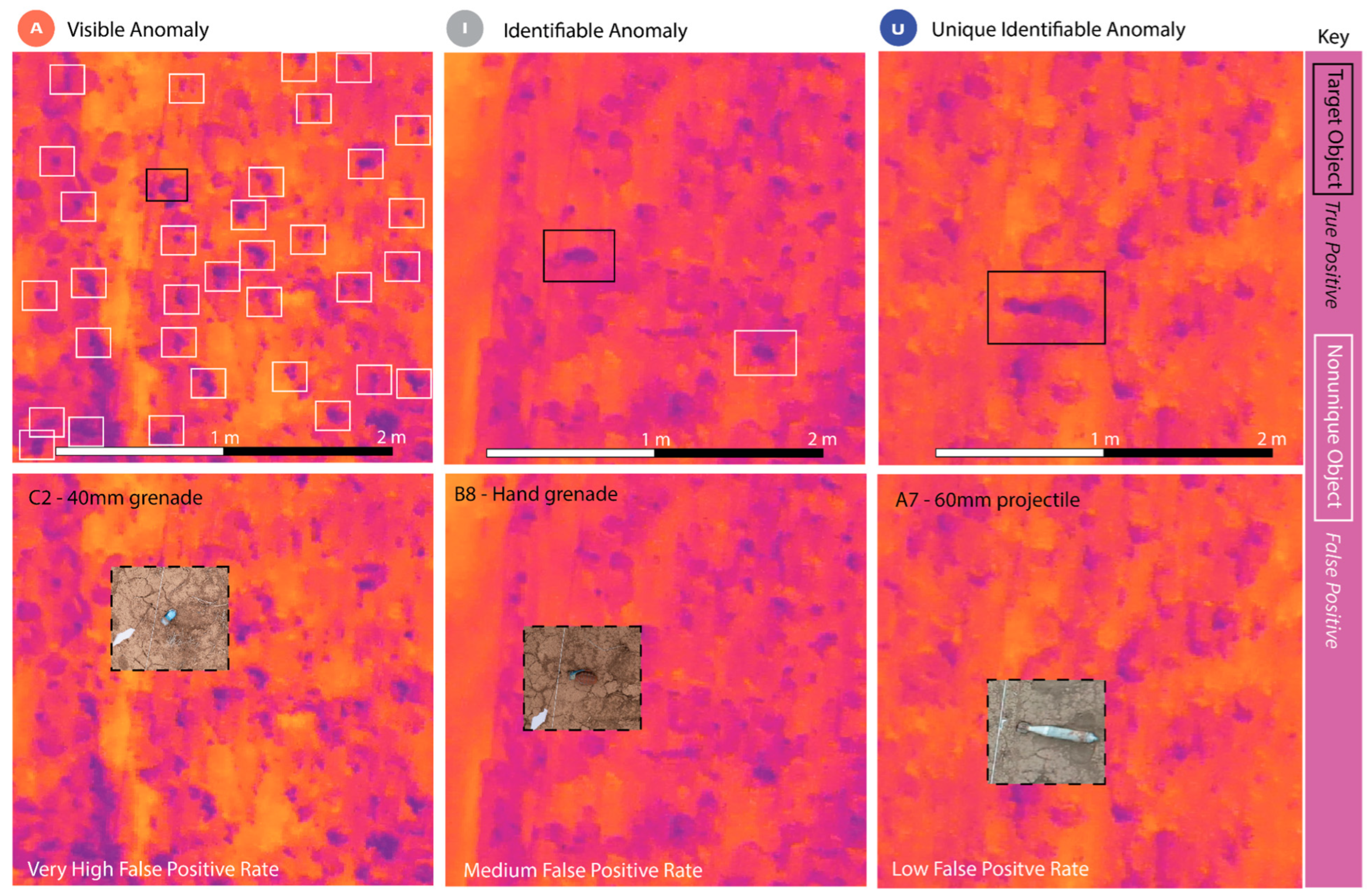
2.1. The AIU Index

In this section we will clearly define the AIU Index and how an object of interest can be quickly sorted based on human interpretation into one of the discrimination criteria. Table 1 provides an overview of the visible anomaly, identifiable anomaly, and unique identifiable anomaly classification metrics. In reality, there is not a strict distinction between visible and identifiable anomaly or identifiable and unique identifiable anomaly; thus, Figure 1 shows a gradient between the classifications. Additionally, a percentage of items will never be unique, and thus, the unique identifiable anomaly class would theoretically never reach 100%. Additionally, the AIU Index is not influenced by a target’s abundance. Whether an object is common, rare, or novel, the same discrimination criteria in Table 1 apply.

2.1.1. Visual Anomaly—Level 1

The lowest, most inclusive discrimination criterion is the visible anomaly. A visual anomaly is defined here as any shape, pattern, color, or temperature change in the location of the target that is visually and/or statistically different from the local background. If yes, then that object or target should be classified as an anomaly in this framework. Figure 2 shows a decision tree that can be used to sort an object into one of the three classes with three simple questions.
Essentially every signature that differs from the background above a certain signal-to-noise threshold could be characterized as an anomaly. In this sense there is a very low barrier for an object to be classified as a visual anomaly. For RGB imagery at low-pixel on-target ratios (where the shape and size of an object cannot be reliably determined), color is a main determinant (over size and features) for determining if the object is an anomaly. This biases objects that have bold and unnatural colors that differ from the background environment.

2.1.2. Identifiable Anomaly—Level 2

The next discrimination level in the AIU Index is the identifiable anomaly. The minimum criteria for a signature to be classified as an identifiable anomaly are the presence of a characteristic shape and size or identifiable feature. If an image analyst with the necessary domain knowledge determines that the anomaly has an identifiable shape and size or characteristic features that are indicative of that item, it can be classified as an identifiable anomaly. In a study on human perception, Biederman found that edges are the most critical component for object recognition, with color, brightness, and texture acting as secondary components, thus forming the basis for an identifiable anomaly [18]. Wang et al., 2004, developed an objective image quality metric based on human visual perception called the Structural Similarity Index, stating that the structural preservation of an image is more important than preserving the luminance or contrast components on human perception of image quality [19]. Extending this idea into object detection or recognition, it further demonstrates that edges and other structural components (shape and size) are of first-order importance for the identification of an object. These identifiable features are not required to be unique, and what is considered identifiable can be subjective. This is why the gradient between the different classifications is blurred in Figure 1 and thus is dependent on the classification task (whether it is beneficial to be more inclusive or exclusive). In one case, the motion of the camera may cause the shape and size of an object to become blurred, making the distinction between anomaly and identifiable anomaly difficult. Items that are characterized as visually ambiguous or non-unique, but still have an identifiable shape and size, fall into Level 2, whereas visually ambiguous objects that lack a characteristic shape or size of a target would fall into Level 1, visible anomaly.

2.1.3. Unique Identifiable Anomaly—Level 3
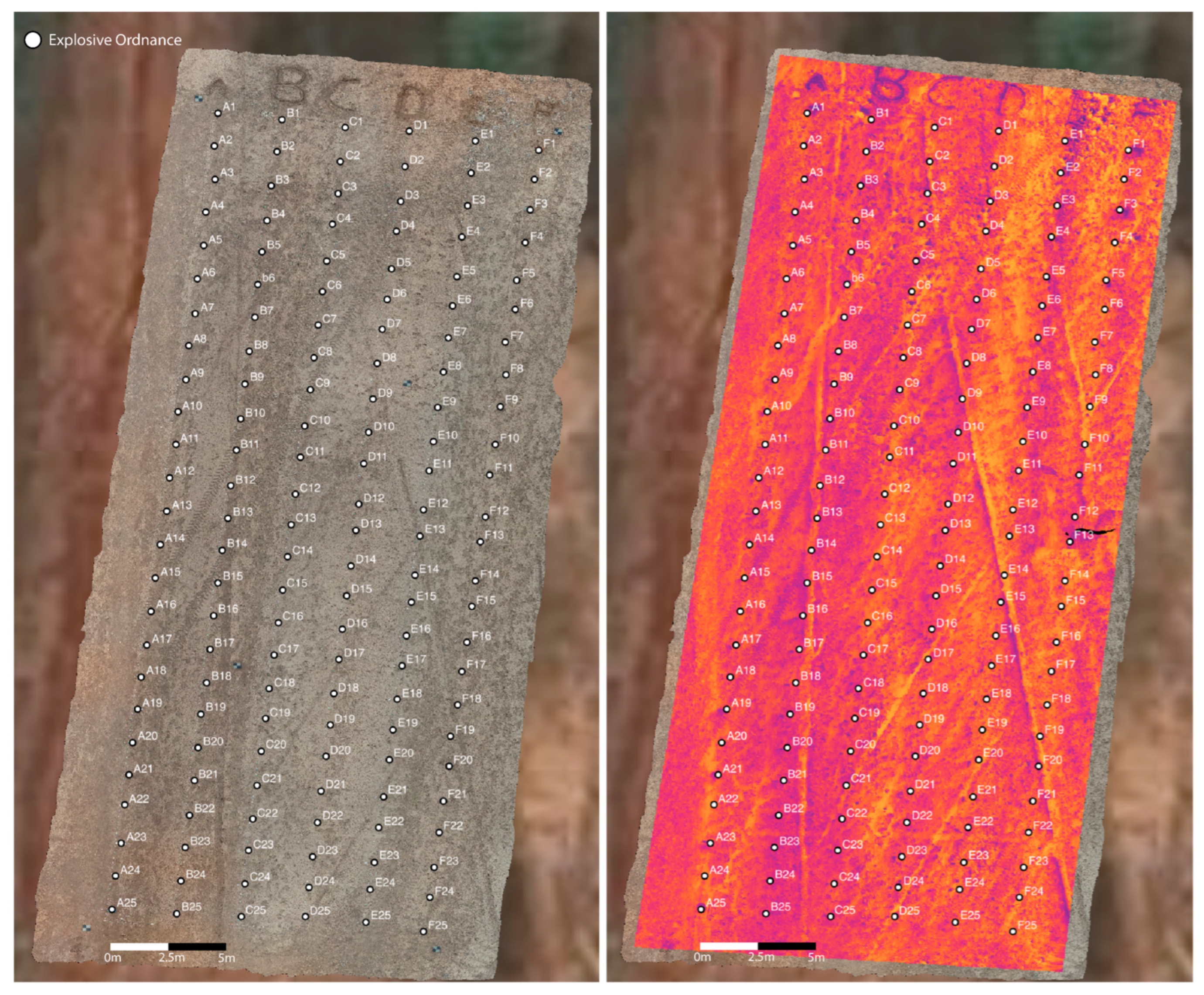
The unique identifiable anomaly is the highest level of discrimination in the AIU Index, with the lowest false alarm rate per detection and the highest confidence. To determine if an anomaly falls into this category, consider the following questions: Is the visual anomaly identifiable and unique to that item? Can it be easily confused with other objects that would be considered false positives? Uniqueness is object and context-dependent. For example, some landmines like the PMN-1 are short black cylinders that, at most resolutions, look like hockey pucks from above, and only at extremely high resolutions are unique if detailed features can be discerned. In general, the PMN-1 will never be unique, whereas a mortar has very distinct and identifiable features even at lower resolutions. Figure 1 shows the conceptual relationship between the three classifications as a function of pixels on target with corresponding detection rates.

2.2. Test Site

The development of the anomaly, identifiable anomaly, and unique identifiable anomaly classification arose from the need to compare visual, thermal, and multispectral datasets collected over a seeded minefield for the purpose of UAV-based landmine detection. The seeded field used for this study is located at OSU’s Center for Fire and Explosives, Forensic Investigation, Training, and Research range in Pawnee, Oklahoma. It was designed and is operated by the U.S.-based non-profit the Demining Research Community in partnership with Oklahoma State University Global Consortium for Explosive Hazard Mitigation [20]. The seeded field consists of 143 inert landmines and UXO spanning a wide range of explosive ordnance. The items are shown in Figure 3 in a condensed grid pattern, but in the actual field, the object rows (1–25) are spaced 1 m apart, and the columns (A–F) are 2 m apart. In the field there are 31 grenades, 27 anti-personnel mines, 25 projectiles, 11 pieces of metallic clutter, 10 3D-printed explosive remnants of war, 10 shells or casings, 9 submunitions, 8 control holes, 7 improvised explosive devices, 2 anti-tank mines, and 1 TNT stick providing a wide breadth of targets to assess the AIU Index for object detection. The datasets for this study were collected over 2.5 years in three separate fields. Field 1 refers to the field seeded in March 2023, Field 2 refers to the field seeded in a different location in June 2023, and Field 3 refers to the field seeded in June 2024. The objects in Fields 1, 2, and 3 are all in the same relative position to each other. The total number of visible surface items varies (from 31 to 143) since many of them were either buried or covered with vegetation at different times during the seeded field’s lifecycle. Note that the image resolution varies due to different sensor types and oscillating flight heights from the wind. Objects that were covered completely by soil or vegetation were removed from the analysis to only compare visible surface items.

2.3. Data Collection

Twelve datasets were collected in total over the seeded fields, including six RGB flights, five TIR flights, and one multispectral flight (Table 2). The RGB imagery datasets used for the analysis were collected using the Autel Dual EVO II visual camera (Autel Robotics, Bothell, WA, USA) and the DJI Mavic 3E wide-angle camera (SZ DJI Technology Co., Ltd., Shenzhen, China). Both the EVO II and Mavic 3E flights were programmed in their internal Autel Explorer V2 app (v2.0.27) and DJI Pilot 2 app (v6.1.1.1) flight planning software built into the handheld controllers. The flight parameters consisted of 80% front overlap, 75% side overlap at 12 m flight height, with flight speed resulting in a ground-sampling distance (GSD) of 0.21 cm/pixel for the RGB imagery and 0.37 cm/pixel for the EVO II TIR imagery. The multispectral data was captured with the four band (NIR, Red Edge, Red, Green) Parrot Sequoia multispectral sensor (Parrot SA, Paris, France) for precision agriculture attached to the DJI Phantom 3 Pro quadcopter (SZ DJI Technology Co., Ltd., Shenzhen, China). The Phantom 3 Pro was flown at 12 m height in a grid-style pattern using the UgCS flight planning software (v4.3) with 80% front overlap, 75% sidelap, resulting in a GSD of 1.17 cm/pixel. Each imagery dataset has an associated dataset ID as part of the larger data release on sensor modalities at the Demining Research Community seeded field shown in Table 2.

2.4. Data Processing

After the imagery was captured, each flight was processed using the commercial structure-from-motion photogrammetry software Pix4DMapper (v4.8.4) to create orthomosaics of the surveyed area. We used the 3D Maps template with default options for the RGB imagery, the Ag Multispectral template for the multispectral imagery, and the Thermal Camera template with default options for the thermal imagery to process the orthomosaics and reflectance maps [22]. After the photogrammetry step, each orthomosaic was uploaded into QGIS. Next, the orthomosaics were georeferenced using the Layer -> Georeferencer tool by clicking the center of the six ground-control points in the orthomosaic and inputting their corresponding Trimble GNSS locations, applying a linear transformation. After the orthomosaics were georeferenced, the edges were clipped to fit the site polygon using the “Clip Raster by Mask Layer” tool in order to produce clean rectangular orthomosaics of each field. All datasets are available for download at https://doi.org/10.5281/zenodo.15324498 [21].

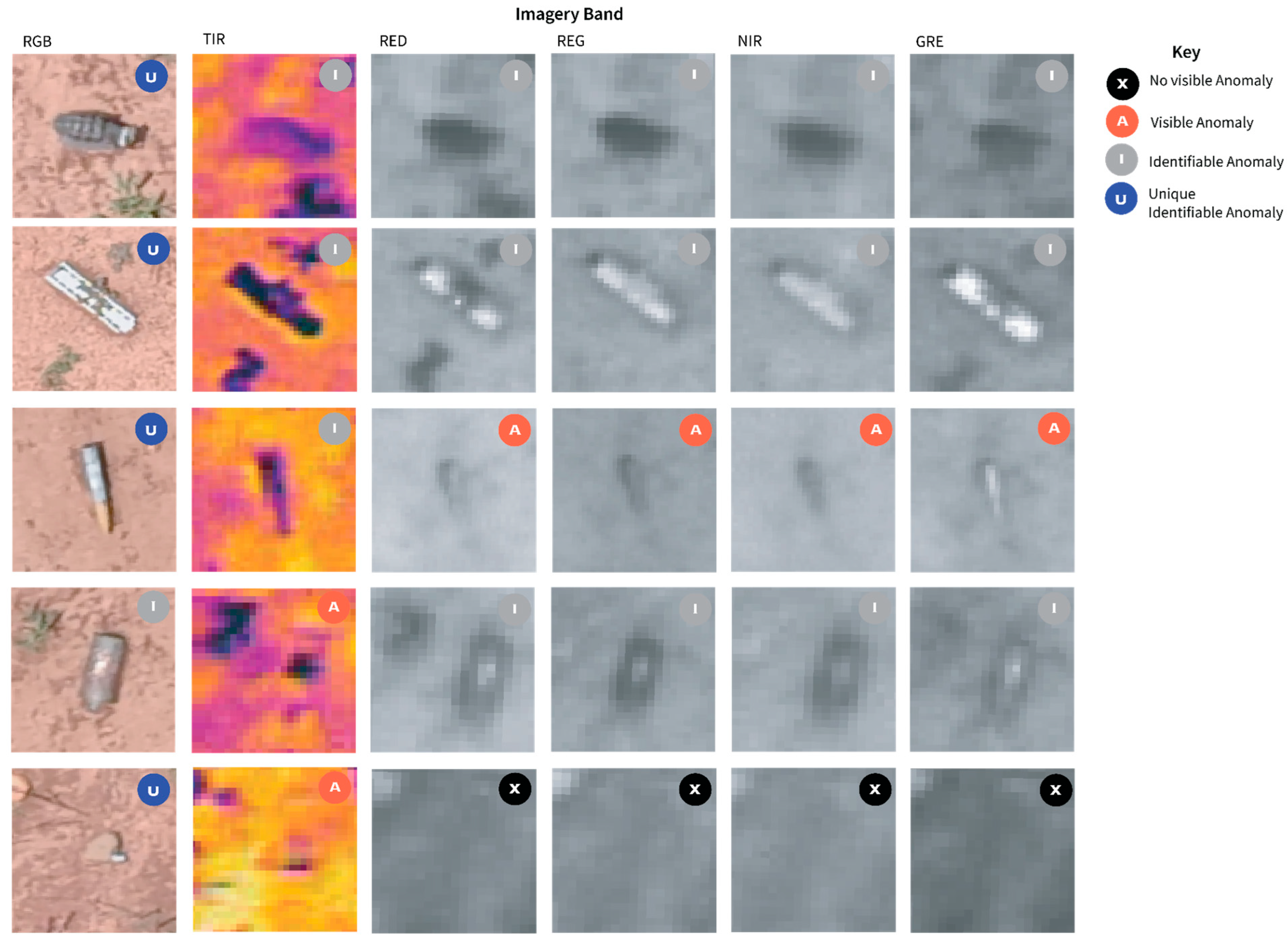
2.5. AIU Analysis for Across Sensor Modalities

For all processed orthomosaics of the seeded field, each of the 143 visible surface items was inspected in QGIS and classified as visible anomaly, identifiable anomaly, or unique identifiable anomaly using the decision criteria in Table 1. Each of the four bands (Red, Green, NIR, Red Edge) in the multispectral imagery separately underwent the same classification process to determine the appropriate discrimination level for each item.
Since the AIU framework is highly dependent on resolution, we compare detection rates across modalities based on pixels on target to yield a resolution-invariant analysis. To achieve this, one of the RGB orthomosaics collected using the DJI Mavic 3E was downsampled four times from 0.21 cm/pix to 0.5, 1.0, 2.0, and 4.0 cm/pix. We repeated the classification process for each object using the AIU Index in order to more thoroughly examine how resolution affects object identifiability and uniqueness. The same analysis was conducted for one of the TIR orthomosaics collected using the Autel Evo II Dual, downsampled from a resolution of 1.0 cm/pix to 2.0 and 4.0 cm/pix. In order to assess the relationship between pixels on target and detection classification, the surface area for each object was measured in QGIS using the Measure Area tool by drawing polygons around the objects. This resulted in the area in cm2, which we multiplied by the orthomosaic resolution (cm/pix), treating the pixel as a square, allowing us to calculate the pixels on target. Using a Python (v3.10) script, the columns for anomaly, identifiable anomaly, and unique identifiable anomaly were converted into a binary format, with “Yes” assigned a value of 1 and “No” assigned a value of 0. Then we applied a rolling mean with a window size of 50 observations and a minimum of 25 data points to compute the mean detection rates for anomalies, identifiability, and uniqueness. Since the input data was binary, the rolling mean analysis was required to relate the detection rate to pixels on target. We choose the window size of 50 to allow us to derive 50 distinct detection rate values spanning 0 to 100% (at 2% increments) and to ensure smoothing over the diverse objects in the seeded field, minimizing the impact of anomalous objects. This analysis was conducted separately for the visual and TIR imagery datasets.

2.6. Flight Height Relationship to Identification Rate

The next experiment was to determine the relationship between UAV flight height and the likelihood of target identification in RGB imagery. To achieve this, we derived an equation that relates flight altitude to pixels on target for a particular object of interest. This allowed us to quantify how the detection rate (in this case, identifiable anomalies) varies with altitude across common UAV RGB camera payloads used in aerial surveys. The ability to detect an object from aerial imagery depends on the resolution or GSD (ground sample distance), which is the real-world size of a single image pixel. The GSD of a nadir UAV survey can be calculated as follows:
G S D = s e n s o r   w i d t h     f l i g h t   h e i g h t i m a g e   w i d t h     f o c a l   l e n g t h  
where GSD has units of (m/pixel), flight height is the UAV flight height (m), sensor width is the physical width of the camera sensor (mm), image width in pixels, and focal length is the camera’s focal length (mm). A target object, such as a landmine in this case study, has a known real-world surface area A (cm2). For simplification, assuming a square object, the object side length can be computed as follows: object length = √A /100 (m). At a given GSD (m/pix) and a defined target object area (cm2), pixels on target (P) can be computed as follows:
P = ( o b j e c t   l e n g t h G S D ) 2
Rearranging Equation (2) to solve for GSD and substituting it in for GSD in Equation (2), we derive the equation solving for flight height:
F l i g h t   H e i g h t =   i m a g e   w i d t h     f o c a l   l e n g t h     o b j e c t   l e n g t h       s e n s o r   w i d t h     P
which relates flight height to the pixels on target for a given UAS. We then plug in the empirically derived rolling mean pixels on target required to classify a target object (in this case, landmines and UXO) as an identifiable anomaly by 10% intervals from 10 to 100% calculated in Section 3.1. We applied Equation (3) to the camera parameters of the four common quadcopter UAVs: the DJI Mavic 3E, DJI Phantom 4 (SZ DJI Technology Co., Ltd., Shenzhen, China), Autel EVO II Dual (Autel Robotics, Bothell, WA, USA), and Skydio X2 (Skydio, Inc., Redwood City, CA, USA). This model provides a quantitative foundation for evaluating the impact of UAV flight altitude on identifiable anomaly detection rates and serves as a baseline for selecting optimal survey heights for aerial object identification.

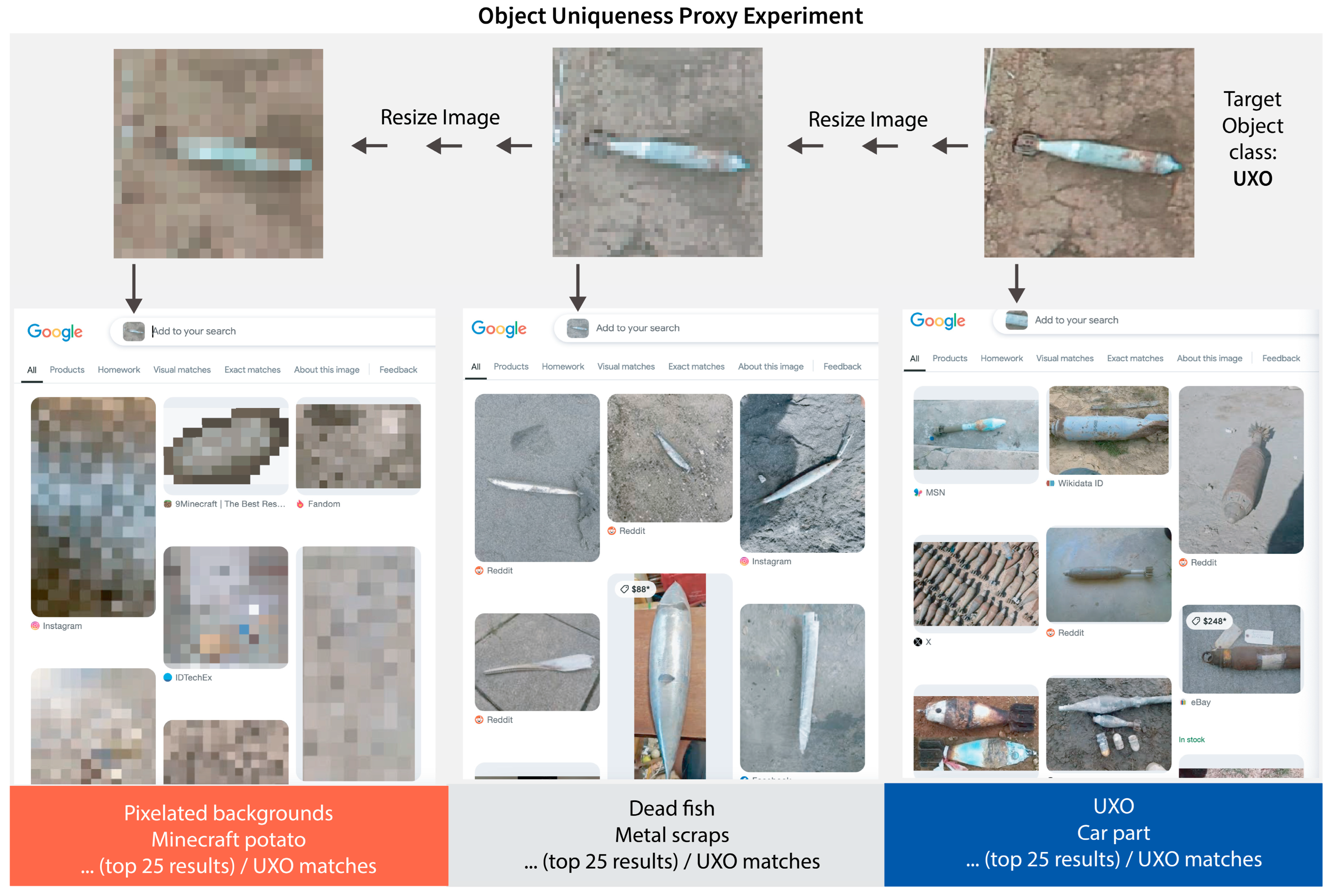
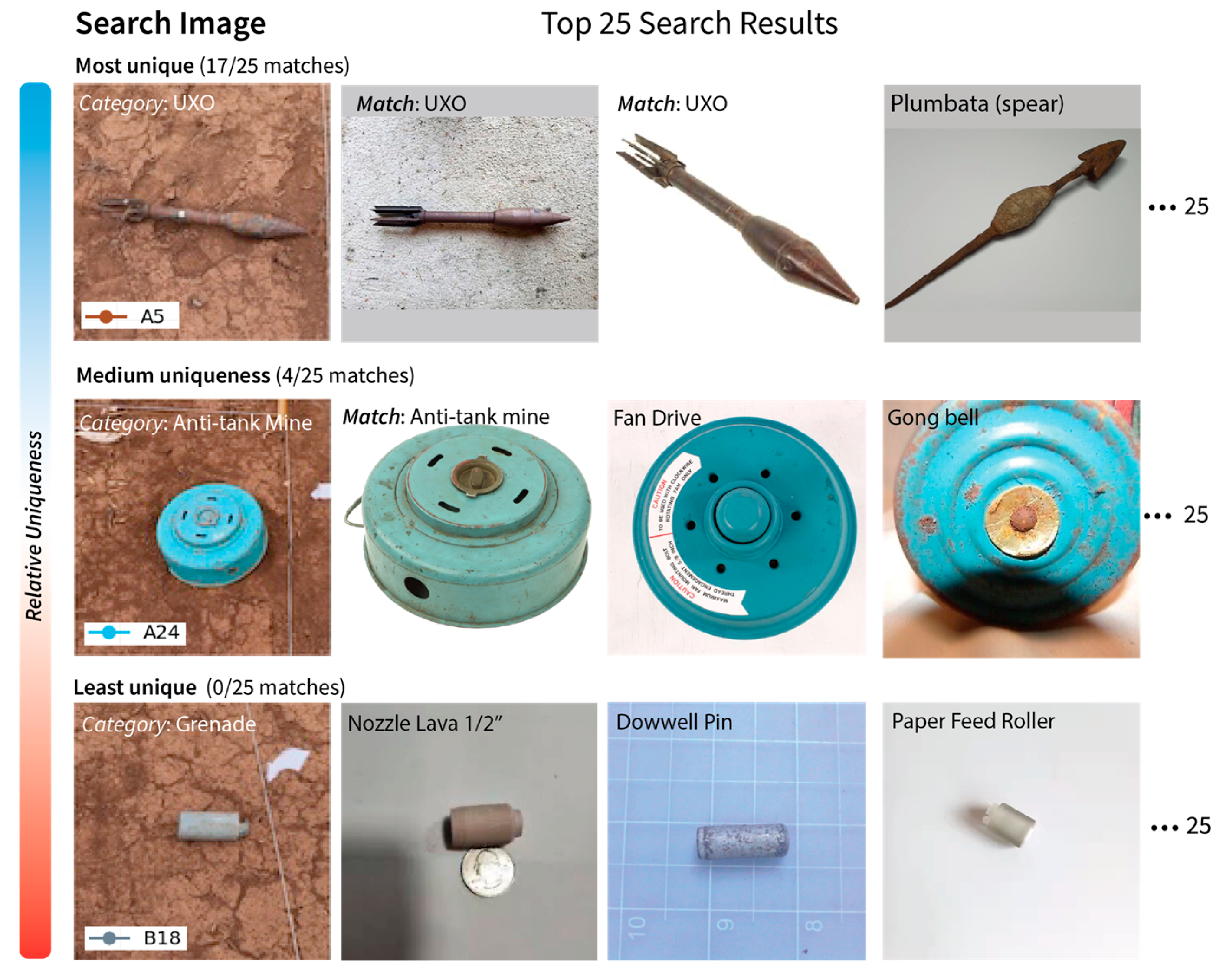
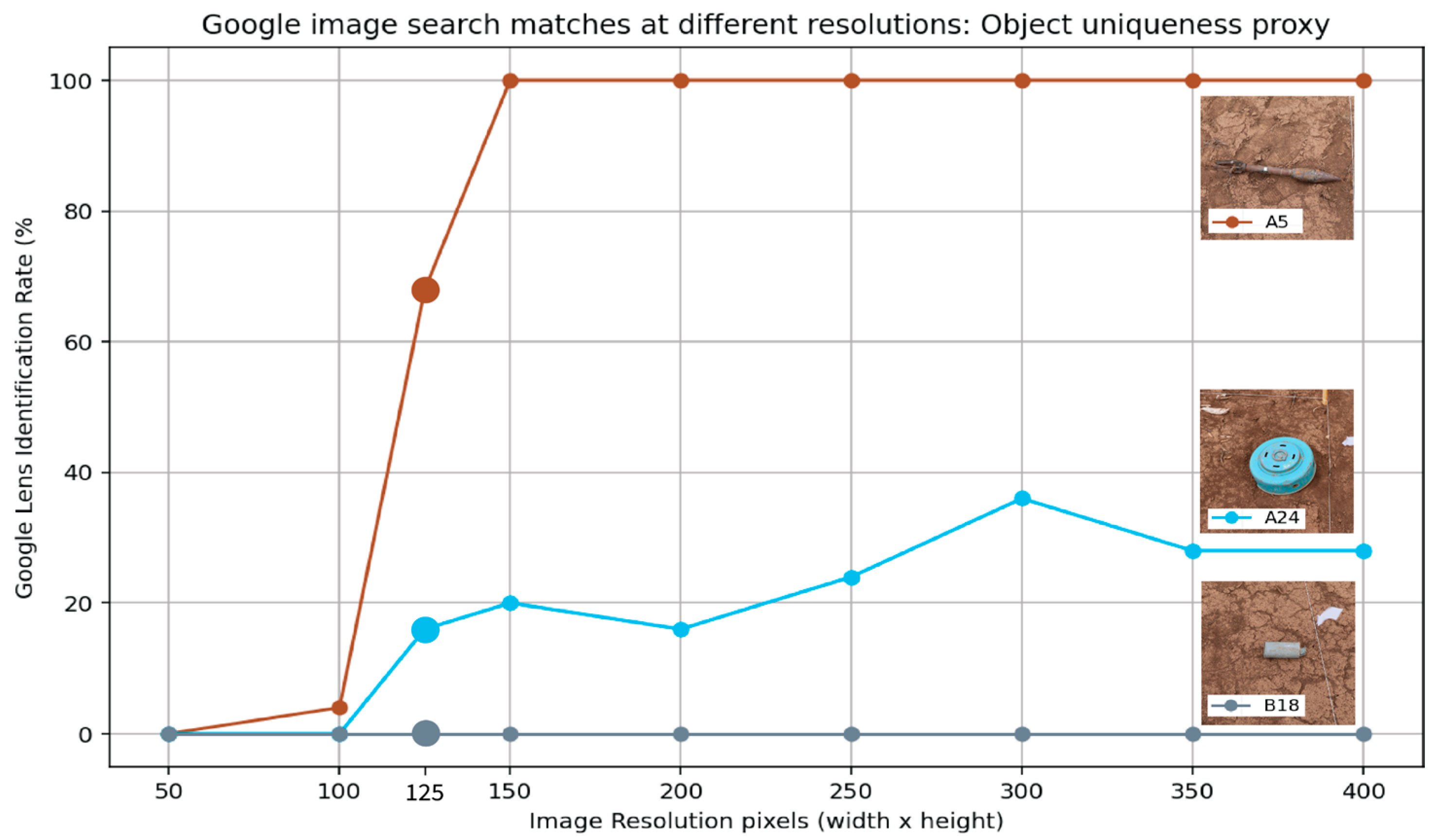
2.7. Object Uniqueness Investigation

Object uniqueness is a property that is very difficult to quantify. The uniqueness metric, as determined by human interpretability, is subject to human bias, exposure to similar-looking items, object commonality, and expertise in identifying the target object features. In order to obtain an independent proxy for object uniqueness separate from the author’s bias of known and familiar objects, we devised an experiment where we selected three objects of various perceived uniqueness on what we believe would be endmembers for object uniqueness. The three objects from the seeded field were the M6A1 projectile, the M12AI anti-tank mine, and the Handgranate 343d grenade with corresponding broad classes defined to be UXO, landmine, and UXO (grenade). For the three selected objects, we cropped an area centered on the objects and downsampled the image to 400 × 400 pixels. These 400 × 400 pixel images were resized down to 50 × 50 pixels in 50 pixel increments (400 × 400, 350 × 350, … 50 × 50 pixels). Each image was then input into Google Lens image search to determine the percentage of the top 25 search results that matched the object’s broad class. We decided to use this method as an independent metric for object uniqueness because the internet has a very wide sampling of objects that could be non-unique matches of the input images. Figure 4 illustrates the workflow graphically.

3. Results

3.1. Comparing RGB, Thermal, and Multispectral Imagery for Landmine Detection

In this section we compare the results of 12 separate UAV surveys over the seeded minefield. Figure 5 shows one of the processed RGB orthomosaics next to the TIR orthomosaic of the same field.
Visual inspection of the RGB datasets resulted in 100% (382/382) of the visible surface targets aggregated across all different flights were classified as visible anomalies, 96.6% (369/382) as identifiable anomalies, and 47.6% (182/382) as unique identifiable anomalies with an object count weighted mean resolution of 0.27 cm/pix (excluding buried or hidden objects). The TIR targets were classified as 96.0% (237/247) visible anomalies, 26.3% (65/247) as identifiable anomalies, and 1.6% (4/247) as unique identifiable anomalies with an object count weighted mean resolution of 0.90 cm/pix. The target objects in the Parrot Sequoia multispectral bands were classified as 83.3% (100/120) visible anomalies, 42.5% (51/120) as identifiable anomalies, and 0% (0/120) as unique identifiable anomalies with a resolution of 1.17 cm/pix.
These results reflect that at an equal flight height of 12 m, RGB imagery had the highest detection rate in all AIU classes, followed by thermal and multispectral imagery. The multispectral datasets had the lowest unique identifiable anomalies and visible anomalies, while the thermal imagery had the lowest percentage of identifiable anomalies. Figure 6 shows zoomed-in RGB, thermal, and multispectral imagery of five different items from the seeded minefield classified with the AIU Index.
Context is crucial for determining if an object is an anomaly or an identifiable anomaly. Figure 7 illustrates that a zoomed-out view of the thermal imagery provides useful background context to help determine the AIU classification of the object. Notice how the 40 mm grenade is categorized as a visible anomaly, with many false positive non-unique signatures, whereas the 60 mm projectile has no false positives and is a unique identifiable anomaly.
The flights analyzed in this study have different resolutions resulting from flight height and sensor type. As image resolution increases, the interpretability of an object shifts from visual anomaly, to identifiable anomaly, to unique identifiable anomaly. This means that as resolution increases, the detection rate increases and the false positive rate decreases.
Figure 8 shows the detection rate for the AIU Index as a function of (50 rolling mean value) pixels on target for the RGB and thermal datasets. The visual imagery achieved 100% visible anomaly detection at 23 pixels on target, and 100% identification at 125 pixels on target. Not all objects are inherently visually unique, and thus, given the objects in the minefield, at 250 pixels on target, approximately 60% were classified as unique identifiable anomalies. The thermal imagery achieved 100% visible anomaly detection at 35 pixels on target and 60% identification rate at 200 pixels on target. Interestingly, almost none of the objects present in the thermal imagery were visually unique, instead appearing as thermal blobs roughly the shape and size of the target object. This means that at the same resolution, visual imagery has higher confidence and lower false positive rates compared to thermal imagery for detecting landmines and UXO. In order to achieve the same detection accuracy, thermal requires more pixels on target to identify an object.
In remote sensing applications for thermal imagery, to obtain the same confidence of identification as visual imagery, the UAV must fly at a lower altitude for two reasons. The first is that thermal cameras inherently collect lower resolution at the same flight height as most RGB cameras, and the second is that the objects themselves are less identifiable in the thermal imagery at the same pixels on target. The combination of both these facts results in thermal cameras being more expensive, providing less value per pixel, and covering less area in the same amount of time as opposed to their RGB counterparts. This is because thermal identification requires thermal contrast between the target object and the background environment, which may result from material properties such as emissivity, thermal conductivity, or environmental factors such as the differential apparent thermal inertia [23,24]. In many remote sensing applications, the thermal contrast of objects may be small or non-existent compared to the background, as most objects thermally equilibrate with the background environment over the diurnal cycle [25,26]. Collection of TIR imagery during hours with the greatest temperature swing, such as just after sunrise or before sunset, has been shown to improve thermal contrast of small objects such as landmines due to the differential apparent thermal inertia [27]. Contrast between the environment and a target object in RGB imagery is primarily dependent on the color of the object and remains stable throughout daytime hours. Additionally, RGB imagery provides a full color spectrum (three bands) as opposed to TIR, which is a single band, resulting in improved disambiguation of small objects in RGB imagery.

3.2. Relationship Between Flight Height and Detection Rate

In this section we demonstrate how the AIU detection rate curves calculated in Figure 8 can be used to determine flight height for an object of a specified size. Given a target object size for a specific UAV, the optimal flight height for a desired identification rate (Level 2, identifiable anomaly) between 0 and 100% can be calculated. Figure 9 shows identification rate curves in 10% intervals as a function of flight height and object size for the DJI Mavic 3E wide-angle camera. This plot can be used to estimate the utility of previously collected data to determine if it meets the specified detection rate requirements or for future mission planning for calculating the optimal flight height. Note this plot does not take into account external factors such as motion blur at lower altitudes and atmospheric effects at higher altitudes, but provides a first-order approximation based on resolution changes with altitude.

3.3. Proxy for Object Uniqueness

Figure 10 shows the three objects (UXO, anti-tank mine, and grenade) chosen from our dataset. We find that the UXO (item A5) had the highest match rate using reverse image search at every given image resolution. At the 125 × 125 pixel resolution, the first mismatches for the UXO arose, with 17/25 of the top search images being UXO matches and 8 of them being visually similar objects like rusty spears and arrowheads.
We find that besides the object’s properties, resolution highly corresponds with object uniqueness. At extremely high resolutions, the smallest details, such as individual serial numbers, can be read. At a resolution of 1 pixel, non-uniqueness converges to a maximum. For an 8-bit single band pixel, there are only 256 unique values that would represent every known object, presenting extreme non-uniqueness. Figure 11 shows that as the image resolution decreases, the uniqueness in terms of search result matches decreases. While quantifying object uniqueness is difficult, highly subjective, and context-dependent, we find that (1) uniqueness increases with increasing resolution, and (2) certain objects have distinguishable features that make them more unique than objects that have a similar shape, size, and features to many other objects.

4. Discussion

4.1. Limitations and Discussion on Object Uniqueness

One limitation in the Google image search methodology is that object commonality and popularity will bias the search results, outputting more common or popular objects than a true sampling of all non-unique images of different classes. Additionally, while many objects may exhibit non-unique signatures (especially certain modalities), context and background environment are essential for determining if an object is a likely target or not. For example, if there is an object that looks like a circular landmine, but it is in the middle of a busy grocery store in America, then the odds are extremely low for that non-unique item to actually be a landmine. If that same object was found in a confirmed hazardous area, the probability that it is a landmine is much higher. In this sense, the difficulty posed by non-uniqueness can be mitigated by context and prior information. Applying this logic, object uniqueness can be constrained for many tasks to the prediction domain.

4.2. Evaluating Object Detection Across Sensor Modalities Using the AIU Index

The AIU Index provides the ability to quantitatively assess the value of each pixel in one modality to another, as shown in Figure 8. By controlling for object size and moving from the resolution space to the pixel-on-target space by multiplying surface area of the target object by the pixel area at a given resolution, one can then compare the required number of pixels for each modality (thermal, visual, multispectral, ect.) required to detect an anomaly, identify the target, and uniquely identify the target. We found that for the use-case of surface detection of landmines and UXO, the value of an RGB pixel provided greater utility for detection than thermal or multispectral imaging at the same number of pixels on target. This has major implications in mission planning for determining necessary flight height and resolution to collect data for each modality, as well as cost–benefit analysis for determining what modalities to use on a given task. In general, RGB cameras collect higher resolution imagery at the same flight height, are significantly cheaper than their thermal or multispectral counterparts, and require less expertise to analyze and process. Without this apples-to-apples (or pixel-to-pixel) comparison, this value assessment would be difficult to make.
It is important to note that visual, thermal, and multispectral all have different internal and external variables that will influence detection rate for landmine detection and other object detection tasks. For thermal imagery, some external factors that affect landmine detection are the time of day and daily temperature changes (ground temperatures can change drastically between day and night affecting the differential apparent thermal inertia of the objects), weather conditions (rain, fog, or high humidity can influence thermal readings), soil moisture content (affects heat retention in the ground) and thermal properties such as emissivity of target object [23,24]. Therefore, the results of this study are relevant for the conditions in Oklahoma in which the data were collected.
The AIU Index can be extended to other domains outside of imagery as long as the signals can be classified by a domain expert. Each modality will have different properties, such as spatial or spectral resolution, that will determine if an object can be distinguished from the background environment. Some modalities will never be able to discern if a target is an identifiable or unique anomaly with current techniques. For example, a handheld metal detector will make a beep if it passes over a metallic object. This signal or beep would be categorized as an anomaly (Level 1), but there is no way to reliably know the type of object and if it is unique. In this modality, the detection characterization may be moved to any anomaly (above a certain noise threshold), whereas in imagery, the detection threshold will be placed at an identifiable anomaly (Level 2).

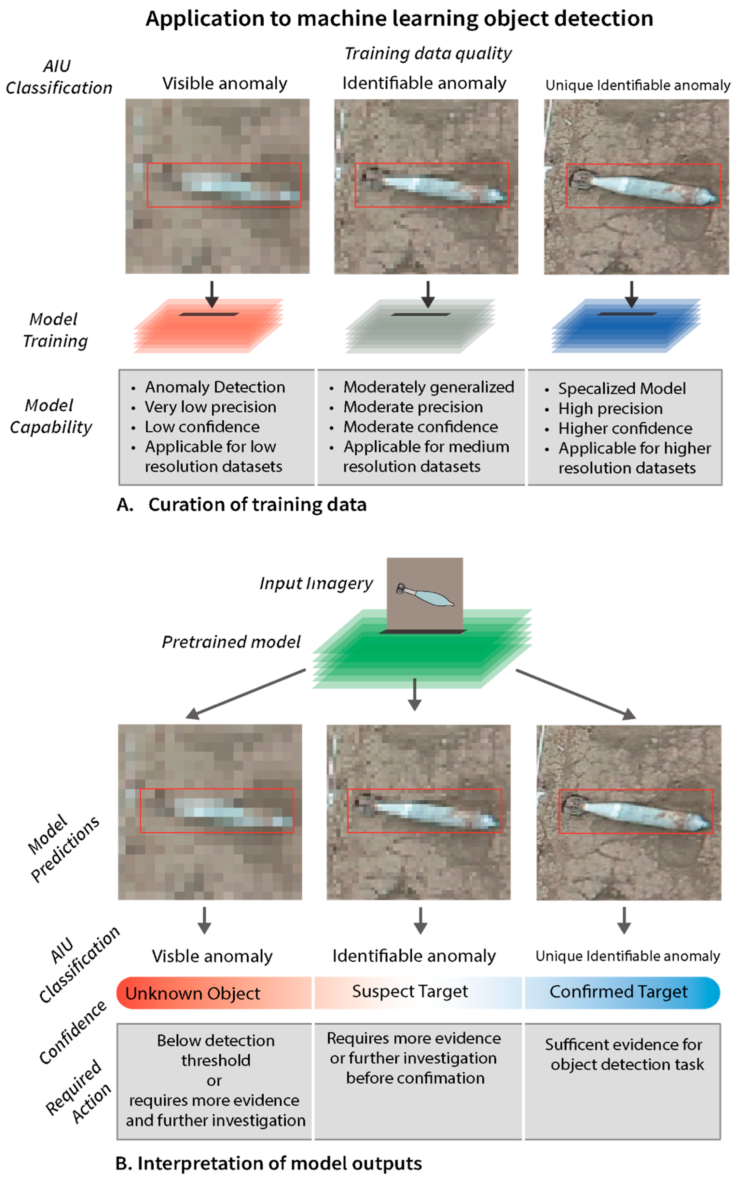
4.3. Application to Machine Learning

4.3.1. Comparing AIU to Precision and Other Object Detection Metrics

Standard object detection evaluation metrics such as precision, recall, F1-score, and mean average precision (mAP) do not consider object uniqueness or the ambiguousness of a target. Precision is the ratio of true positives to the number of total predictions (sum of true positives and false positives). While precision measures the ratio of false positives, it does not diagnose the root cause of why those false positives are there in the first place. We hypothesize, precision is related to the AIU classification because highly non-unique objects will have a higher false positive rate and lower precision than unique objects. False positives may arise from the model being too generalized, resulting in a model that includes too many predictions of a different class than the target class, or the target objects are non-unique and visually overlap with other similar objects. The first issue can be mitigated with a robust training dataset that has well-balanced generalization to overfitting, but the non-unique or visually ambiguous issue cannot be solved with data or new architectures. Due to this, the AIU Index can provide extremely valuable information on the underlying false positive causes. Both metrics can be combined by classifying the percentage of labels in the dataset as anomalies, identifiable anomalies, or unique identifiable anomalies, and comparing the precision versus the AIU percentages. If precision is low (high ratio of false positives) but a high percentage of labels are classified as unique identifiable anomalies (level 3), then the model is likely too generalized and needs to train longer. If precision is low and uniqueness (level 3) is low, then the problem likely stems from the training data itself as opposed to over-generalization of the model. A less common metric called Probability-based Detection Quality (PDQ), proposed by Hall et al. 2020 [28], incorporates spatial and label uncertainty into the evaluation of each prediction, considering multiple class label matches for each prediction. This has implications for assessing the uniqueness or ambiguity of a prediction (by evaluating the number of matching labels), so PDQ may serve as a complementary metric to diagnose whether low precision is due to over-generalization or inherent non-uniqueness of the objects. On the instance-level, prediction score, or the confidence the machine learning model has for each prediction, may correlate with the AIU levels (low score being associated with anomalies and high score corresponding to unique identifiable anomalies), but this relationship requires future experimentation.

4.3.2. Training Data

Training data fidelity is of utmost importance for building effective machine learning models. The classic machine learning cliché, “garbage in, garbage out”, emphasizes that determining what data should be used for training is essential. One of the major challenges in object detection is making generalized models for a particular object class that are robust to changes in lighting, view angle, background, and intra-class variance, while not overfitting the model to the training data [29,30,31,32]. The input training data, loss function, number of training epochs, and other variables dictate the delicate balance between making a model robust to variance, but not making it too generalized. We speculate that models trained on non-unique objects or objects that are very similar visually to another struggle with precision in false-positive-rich environments; hence, object uniqueness in the source domain is correlated with the false positive rate. Object classes that do not visually overlap with any other objects can be effectively trained to be more generalized models without reducing precision. Focusing on image-based object detection, if the training data is broken into the visible anomaly, identifiable anomaly, and unique identifiable anomaly, the model’s capability will reflect the training data’s AIU classification. Figure 12A illustrates how training on the different classes would result in different precisions and model capabilities. Training on objects that are classified as visible anomalies may produce a very low precision (many false positives) and a high recall model, suitable for simple anomaly detection in resolution-limited tasks. Training on identifiable anomalies (objects that have a characteristic shape and size but are not unique) could lead to a decrease in precision compared to solely unique identifiable objects, but may improve recall in situations where target objects do not have any identifiable features but have an apparent shape and size. In applications where a false negative is more damaging than a false positive, like landmine detection, this may be a worthy trade-off. Training on only unique identifiable anomalies would result in highly specialized models with high precision (low false positive rates) but may struggle with broader generalization and generally require more pixels on target. It is possible to mitigate the generalization issue for unique identifiable targets by training the classes to be more generalized and more robust to variance without the risk of decreasing precision if the target object is not visually similar to any other objects in the source domain.
Future work can investigate how the training data in the different AIU Index levels affect recall and precision and investigate the tradeoffs between overfitting versus generalization for unique and non-unique objects. An experiment involving training three separate object detection models exclusively on Level 1, 2, or 3 could quantify the impact of training on different AIU levels on model precision. Such work could also compare AIU-level-specific training to a mixed training dataset as a control, providing an empirical foundation for the AIU framework’s utility in model development.
Certain architectures, such as those that incorporate feature-pyramid networks, are able to detect objects at multiple scales, downsampling the training data at multiple scales to make the model more robust and scale invariant [33]. With these methods, it is possible that models trained on high-resolution unique identifiable targets can still detect the same objects that are no longer visually unique (classified as an identifiable anomaly) in some cases. The inherent risk is that precision suffers as objects’ features are blurred and the object becomes less non-unique.

4.3.3. Interpretation of Bounding Boxes

After an object detection model, such as YOLO, outputs a bounding box, this information often requires human decision-making to derive some type of actionable intelligence. If the model predictions are required to be clean (i.e., no false positives), then a human analyst will need to review the predictions. This workflow is common in humanitarian mine action when analyzing drone imagery for landmines using object detection models [6]. This workflow may also benefit medical applications regarding whether a prediction requires further investigation or action for abnormal or cancerous cells in CT images [34,35,36]. Figure 12B shows that the output AIU classification for each prediction has implications on the confidence of that information and the required follow-up action. For example, considering the use-case of landmine detection, an image analyst may discard predictions that are visible anomalies (below the determined detection threshold by the image analyst), mark identifiable anomalies as suspect items that require further investigation before confirmation, and mark unique identifiable anomalies as confirmed detections without the need for further investigation. Certain decisions, such as in-flight UAV actions, may demand real-time or near-real-time adoption of the AIU Index for object detection. The AIU framework allows operators to sort target objects in near-real time, enabling time-sensitive decisions to be made within seconds based on the AIU level. One example could be UAV search and rescue missions using real-time detection models to find a missing person. As a prediction is made, an operator can then characterize the prediction as an identifiable anomaly in the shape of a person, which may prompt further investigation (flying lower with the UAV to achieve higher resolution) until the pilot determines the prediction in question is a unique identifiable anomaly (the person they are searching for) or a false positive. People are likely already passively applying this logic, but the AIU Index can help communicate the certainty and required action for object detection tasks, removing a degree of ambiguity that is not communicated via a bounding box and confidence score. Applying the AIU Index is unnecessary for tasks with high detection confidence, no need for disambiguation, false positives that require no different action than true positives (i.e., counting items), or in controlled environments such as assembly lines and factories where false positive occurrence is negligible [37,38].

4.4. Using the AIU Framework for Data Collection for UAVs

Similar to the purpose of the NIIRS rating, which was developed to inform imagery collection protocol and ensure the collected imagery provided useful intelligence to the end user, the AIU Index can be used to inform UAV-based mission planning to ensure the desired objects can be discerned from the collected imagery. By defining an object of interest and the required AIU rating or corresponding acceptable false alarm rate, this will inform the required resolution to achieve that level of interpretability, and as a consequence, the flight height for a given payload.
For an application such as landmine detection used as the case study for this paper, the AIU curves shown in Figure 9 can be used to determine the specific parameters of your data collection mission. For example, if you want to make sure that at least 90% of the 250 cm2 surface area landmine will be identifiable targets, you will need a minimum of 54 pixels on target corresponding to a flight height above ground level of 80.7 m using the Mavic 3E wide-angle camera. This ability to model the desired interpretability level of the target objects increases mission efficiency by allowing for optimized flight height and payload purchase. Optimal flight height can result in either flying higher and covering more area in less time or flying lower to avoid collecting useless or low-quality data for your task. Figure 13 shows the flight height in meters to achieve the 125-pixel on-target threshold for a 100% identification rate (Level 2) with four popular quadcopter UAVs with built-in RGB cameras.
This figure does not consider motion blur, image graininess and noise, and other suboptimal artifacts resulting from real-world data acquisition. Additionally, this plot assumes fully unoccluded objects, but in the natural world, occlusion due to vegetation, dirt, shadows, and buildings will reduce detection rates dramatically [39,40]. Another limitation of this method is that it does not take into account atmospheric effects or sensor noise, so the real-world identification rates will be lower than what is estimated. Considering real-world complexities, the flight height would need to be slightly lower than what is plotted in Figure 13 to achieve 100% identifiable anomaly, but nonetheless, this figure informs the data acquisition team of the flight height where an image analyst can no longer reliably identify the target object. This workflow can be used to inform the appropriate flight height for surveying or mapping object detection tasks, such as landmine detection or search and rescue.

5. Conclusions

In this paper we proposed the AIU Index, a three-tiered interpretability framework for object detection centered around false positive rates. We demonstrated that the AIU Index has utility in disambiguation for object detection, choosing useful training data for deep learning object detection models, providing a framework for comparing the utility of different sensor modalities, and mission planning for determining optimal data collection protocols for remote sensing systems. We applied the AIU Index on RGB, thermal, and multispectral datasets on a seeded minefield to determine the true detection value of a pixel for each modality for landmine detection. We found that RGB imagery had the highest rate for identification and unique identification for visible surface landmines and UXO compared to thermal or multispectral imagery. Overall, the visible anomaly, identifiable anomaly, unique identifiable anomaly framework should be applied to applications and modalities that are prone to false positives to help communicate the inherent uncertainty regarding non-uniqueness in object detection.

Author Contributions

Conceptualization, J.B.; methodology, J.B.; validation, J.B.; formal analysis, J.B.; investigation, J.B.; data curation, J.B.; writing—original draft preparation, J.B.; writing—review and editing, J.B. and F.O.N.; visualization, J.B.; supervision, F.O.N. All authors have read and agreed to the published version of the manuscript.

Funding

This research received no external funding.

Data Availability Statement

All data used in this study is available at Baur, J., & Steinberg, G. (2025) [21]. Demining Research Community Seeded Field: High-Resolution RGB, Thermal IR, and Multispectral Orthomosaics [Data set]. Zenodo. https://doi.org/10.5281/zenodo.15324498.

Acknowledgments

The authors would like to thank John Frucci from the OSU Global Consortium for Explosive Hazard Mitigation for access to the explosives range and inert ordnance. We would also like to thank Alex Nikulin, Sharifa Karwandyar, and Tim de Smet from Binghamton University for collecting the multispectral data and assistance with the UAVs. Lastly, we would like to thank Gabriel Steinberg from the Demining Research Community for providing edits on the paper and insightful feedback.

Conflicts of Interest

The authors declare no conflicts of interest.

Abbreviations

The following abbreviations are used in this manuscript:
UXOUnexploded Ordnance
DRIDetection, Recognition, Identification

References

  1. Abdelfattah, R.; Wang, X.; Wang, S. Ttpla: An aerial-image dataset for detection and segmentation of transmission towers and power lines. In Proceedings of the Asian Conference on Computer Vision, Macao, China, 4–8 December 2022. [Google Scholar]
  2. Osco, L.P.; de Arruda, M.D.S.; Gonçalves, D.N.; Dias, A.; Batistoti, J.; de Souza, M.; Gomes, F.D.G.; Ramos, A.P.M.; de Castro Jorge, L.A.; Liesenberg, V.; et al. A CNN approach to simultaneously count plants and detect plantation-rows from UAV imagery. ISPRS J. Photogramm. Remote Sens. 2021, 174, 1–17. [Google Scholar] [CrossRef]
  3. Leng, J.; Ye, Y.; Mo, M.; Gao, C.; Gan, J.; Xiao, B.; Gao, X. Recent Advances for Aerial Object Detection: A Survey. ACM Comput. Surv. 2024, 56, 296. [Google Scholar] [CrossRef]
  4. Xu, J.; Fan, X.; Jian, H.; Xu, C.; Bei, W.; Ge, Q.; Zhao, T. YoloOW: A spatial scale adaptive real-time object detection neural network for open water search and rescue from uav aerial imagery. IEEE Trans. Geosci. Remote Sens. 2024, 62, 5623115. [Google Scholar] [CrossRef]
  5. Bejiga, M.B.; Zeggada, A.; Melgani, F. Convolutional neural networks for near real-time object detection from UAV imagery in avalanche search and rescue operations. In Proceedings of the 2016 IEEE International Geoscience and Remote Sensing Symposium (IGARSS), Beijing, China, 10–15 July 2016; pp. 693–696. [Google Scholar]
  6. Baur, J.; Steinberg, G.; Nikulin, A.; Chiu, K.; de Smet, T.S. Applying deep learning to automate UAV-based detection of scatterable landmines. Remote Sens. 2020, 12, 859. [Google Scholar] [CrossRef]
  7. Lee, M.; Choi, M.; Yang, T.; Kim, J.; Kim, J.; Kwon, O.; Cho, N. A study on the advancement of intelligent military drones: Focusing on reconnaissance operations. IEEE Access 2024, 12, 55964–55975. [Google Scholar] [CrossRef]
  8. Carion, N.; Massa, F.; Synnaeve, G.; Usunier, N.; Kirillov, A.; Zagoruyko, S. End-to-end object detection with transformers. In European Conference on Computer Vision; Springer International Publishing: Cham, Switzerland, 2020; pp. 213–229. [Google Scholar]
  9. Redmon, J.; Divvala, S.; Girshick, R.; Farhadi, A. You only look once: Unified, real-time object detection. In Proceedings of the IEEE Conference on Computer Vision and Pattern Recognition, Las Vegas, NV, USA, 27–30 June 2016; pp. 779–788. [Google Scholar]
  10. Ren, S.; He, K.; Girshick, R.; Sun, J. Faster R-CNN: Towards real-time object detection with region proposal networks. IEEE Trans. Pattern Anal. Mach. Intell. 2016, 39, 1137–1149. [Google Scholar] [CrossRef] [PubMed]
  11. Liu, W.; Anguelov, D.; Erhan, D.; Szegedy, C.; Reed, S.; Fu, C.Y.; Berg, A.C. Ssd: Single shot multibox detector. In Computer Vision–ECCV 2016, Proceedings of the 14th European Conference, Amsterdam, The Netherlands, 11–14 October 2016; Part I 14; Springer International Publishing: Berlin/Heidelberg, Germany, 2016; pp. 21–37. [Google Scholar]
  12. Johnson, J. Analysis of image forming systems. Sel. Pap. Infrared Des. Part I II 1985, 513, 761. [Google Scholar]
  13. Driggers, R.G.; Cox, P.G.; Kelley, M. National imagery interpretation rating system and the probabilities of detection, recognition, and identification. Opt. Eng. 1997, 36, 1952–1959. [Google Scholar] [CrossRef]
  14. Çetin, A.E.; Dimitropoulos, K.; Gouverneur, B.; Grammalidis, N.; Günay, O.; Habiboǧlu, Y.H.; Toreyin, B.U.; Verstockt, S. Video fire detection–review. Digit. Signal Process. 2013, 23, 1827–1843. [Google Scholar] [CrossRef]
  15. Havens, K.J.; Sharp, E.J. Thermal Imaging Techniques to Survey and Monitor Animals in the Wild: A Methodology; Academic Press: Cambridge, MA, USA, 2015. [Google Scholar]
  16. Sjaardema, T.A.; Smith, C.S.; Birch, G.C. History and Evolution of the Johnson Criteria (No. SAND2015-6368); Sandia National Lab. (SNL-NM): Albuquerque, NM, USA, 2015. [Google Scholar]
  17. Weldon, W.T.; Hupy, J. Investigating methods for integrating unmanned aerial systems in search and rescue operations. Drones 2020, 4, 38. [Google Scholar] [CrossRef]
  18. Biederman, I. Recognition-by-components: A theory of human image understanding. Psychol. Rev. 1987, 94, 115. [Google Scholar] [CrossRef]
  19. Wang, Z.; Bovik, A.C.; Sheikh, H.R.; Simoncelli, E.P. Image quality assessment: From error visibility to structural similarity. IEEE Trans. Image Process. 2004, 13, 600–612. [Google Scholar] [CrossRef] [PubMed]
  20. Baur, J.; Steinberg, G.; Frucci, J.; Brinkley, A. An accessible seeded field for humanitarian mine action research. J. Conv. Weapons Destr. 2023, 27, 2. [Google Scholar]
  21. Baur, J.; Steinberg, G. Demining Research Community Seeded Field: High-Resolution RGB, Thermal IR, and Multispectral Orthomosaics [Data Set]. Zenodo. Available online: https://zenodo.org/records/15324498 (accessed on 2 May 2025).
  22. Pix4D. What Are the Output Results of Pix4dmapper? 2025. Available online: https://support.pix4d.com/hc/en-us/articles/205327435 (accessed on 2 May 2025).
  23. Jacobs, P.A. Thermal Infrared Characterization of Ground Targets and Backgrounds; SPIE Press: Bellingham, WA, USA, 2006; Volume 70. [Google Scholar]
  24. Nikulin, A.; De Smet, T.S.; Baur, J.; Frazer, W.D.; Abramowitz, J.C. Detection and identification of remnant PFM-1 ‘Butterfly Mines’ with a UAV-based thermal-imaging protocol. Remote Sens. 2018, 10, 1672. [Google Scholar] [CrossRef]
  25. Sabol, D.E.; Gillespie, A.R.; McDonald, E.; Danillina, I. Differential thermal inertia of geological surfaces. In Proceedings of the 2nd Annual International Symposium of Recent Advances in Quantitative Remote Sensing, Torrent, Spain, 25–29 September 2006; pp. 25–29. [Google Scholar]
  26. Zhao, H.; Ji, Z.; Li, N.; Gu, J.; Li, Y. Target detection over the diurnal cycle using a multispectral infrared sensor. Sensors 2016, 17, 56. [Google Scholar] [CrossRef] [PubMed]
  27. de Smet, T.S.; Nikulin, A. Catching “butterflies” in the morning: A new methodology for rapid detection of aerially deployed plastic land mines from UAVs. Lead. Edge 2018, 37, 367–371. [Google Scholar] [CrossRef]
  28. Hall, D.; Dayoub, F.; Skinner, J.; Zhang, H.; Miller, D.; Corke, P.; Carneiro, G.; Angelova, A.; Sünderhauf, N. Probabilistic object detection: Definition and evaluation. In Proceedings of the IEEE/CVF Winter Conference on Applications of Computer Vision, Snowmass Village, CO, USA, 1–5 March 2020; pp. 1031–1040. [Google Scholar]
  29. Girshick, R. Fast r-cnn. In Proceedings of the IEEE International Conference on Computer Vision, Las Vegas, NV, USA, 27–30 June 2016; pp. 1440–1448. [Google Scholar]
  30. Pham, H.N.A.; Triantaphyllou, E. The Impact of Overfitting and Overgeneralization on the Classification Accuracy in Data Mining; Springer: Berlin/Heidelberg, Germany, 2008; pp. 391–431. [Google Scholar]
  31. Cheon, J.; Baek, S.; Paik, S.B. Invariance of object detection in untrained deep neural networks. Front. Comput. Neurosci. 2022, 16, 1030707. [Google Scholar] [CrossRef] [PubMed]
  32. Li, H.; Li, J.; Guan, X.; Liang, B.; Lai, Y.; Luo, X. Research on overfitting of deep learning. In Proceedings of the 2019 15th International Conference on Computational Intelligence and Security (CIS), Macao, China, 13–16 December 2019; pp. 78–81. [Google Scholar]
  33. Lin, T.Y.; Dollár, P.; Girshick, R.; He, K.; Hariharan, B.; Belongie, S. Feature pyramid networks for object detection. In Proceedings of the IEEE Conference on Computer Vision and Pattern Recognition, Honolulu, HI, USA, 21–26 July 2017; pp. 2117–2125. [Google Scholar]
  34. Elakkiya, R.; Teja, K.S.S.; Jegatha Deborah, L.; Bisogni, C.; Medaglia, C. Imaging based cervical cancer diagnostics using small object detection-generative adversarial networks. Multimed. Tools Appl. 2022, 81, 191–207. [Google Scholar] [CrossRef]
  35. Haq, I.; Mazhar, T.; Asif, R.N.; Ghadi, Y.Y.; Ullah, N.; Khan, M.A.; Al-Rasheed, A. YOLO and residual network for colorectal cancer cell detection and counting. Heliyon 2024, 10, e24403. [Google Scholar] [CrossRef]
  36. Hu, H.; Guan, Q.; Chen, S.; Ji, Z.; Lin, Y. Detection and recognition for life state of cell cancer using two-stage cascade CNNs. IEEE/ACM Trans. Comput. Biol. Bioinform. 2017, 17, 887–898. [Google Scholar] [CrossRef]
  37. Kang, Z.; Catal, C.; Tekinerdogan, B. Machine learning applications in production lines: A systematic literature review. Comput. Ind. Eng. 2020, 149, 106773. [Google Scholar] [CrossRef]
  38. Kumar, K.; Kumar, P.; Kshirsagar, V.; Bhalerao, R.H.; Shah, K.; Vaidhya, P.K.; Panda, S.K. A real-time object counting and collecting device for industrial automation process using machine vision. IEEE Sens. J. 2023, 23, 13052–13059. [Google Scholar] [CrossRef]
  39. Baur, J.; Dewey, K.; Steinberg, G.; Nitsche, F.O. Modeling the Effect of Vegetation Coverage on Unmanned Aerial Vehicles-Based Object Detection: A Study in the Minefield Environment. Remote Sens. 2024, 16, 2046. [Google Scholar] [CrossRef]
  40. Pal, M.; Palevičius, P.; Landauskas, M.; Orinaitė, U.; Timofejeva, I.; Ragulskis, M. An overview of challenges associated with automatic detection of concrete cracks in the presence of shadows. Appl. Sci. 2021, 11, 11396. [Google Scholar] [CrossRef]
Figure 1. Conceptual AIU framework for object detection.
Remotesensing 17 02429 g001
Figure 2. Decision tree to use for characterizing an anomaly within the AIU framework.
Remotesensing 17 02429 g002
Figure 3. Condensed grid of objects before burial for visualization of Demining Research Community’s seeded minefield, adapted from Baur et al., 2023 [20].
Remotesensing 17 02429 g003
Figure 4. Methodology for object uniqueness proxy experiment.
Remotesensing 17 02429 g004
Figure 5. RGB dataset (ID 3-1) on the left next to TIR dataset (ID 4-1) on the right, with surface object locations marked by white dots.
Remotesensing 17 02429 g005
Figure 6. Five separate explosive ordnance shown in RGB, TIR, Red, Red Edge, Near Infrared, and Green bands with AIU classifications.
Remotesensing 17 02429 g006
Figure 7. The top panel shows target objects in thermal infrared imagery. The black boxes are around the target objects, and the white boxes are non-unique false positives. The bottom panels show visual imagery overlaid on the thermal imagery.
Remotesensing 17 02429 g007
Figure 8. Detection rate for A, I, and U metrics as a function of pixels on target. The left panel shows the rolling mean results for the visual imagery, and the right panel shows the results for the thermal imagery.
Remotesensing 17 02429 g008
Figure 9. Identification (I) rate curves as a function of object size and flight height with the DJI Mavic 3E.
Remotesensing 17 02429 g009
Figure 10. Search result examples from Google Lens based on the input search image shown in the leftmost column. Each search image was 125 × 125 pixels, and ordered by most unique (top row) to least unique (bottom row).
Remotesensing 17 02429 g010
Figure 11. Google Lens search result matches as a function of input image resolution for the three test objects (A5, A24, and B18).
Remotesensing 17 02429 g011
Figure 12. Application of the AIU Index to machine learning object detection. Panel (A) shows how the curation of training data based on the AIU classification influences model capability. Panel (B) shows how the AIU Index can be applied for the interpretation of bounding box predictions to determine the associated confidence and required action on the prediction level.
Remotesensing 17 02429 g012
Figure 13. Four common UAVs with their corresponding identification rate (Level 2) based on flight height and object size.
Remotesensing 17 02429 g013
Table 1. Discrimination criteria for the AIU Index.
Classification MetricDescriptionFalse PositivesExample
PMN-2 Mine
Visible Anomaly
- Discrimination Level 1
A shape, pattern, or grouping of values that are statistically different from the local or global background. Below threshold for detection criteria for most imagery-based tasks.HighRemotesensing 17 02429 i001
Identifiable Anomaly
- Discrimination Level 2
A visible anomaly that is identifiable with domain knowledge. The object must have either indicative shape and size or visible characteristic feature. Above threshold for detection criteria.MediumRemotesensing 17 02429 i002
Unique Identifiable Anomaly
- Discrimination Level 3
An object with clear, unique identifiable features, shape, or size that can be discerned with a high degree of certainty. Above threshold for detection criteria.LowRemotesensing 17 02429 i003
Table 2. Detection of anomalies, identifiable anomalies, and unique identifiable anomalies in orthophotos across different sensor modalities. The table presents the number of detected, identifiable, and unique identifiable anomalies in RGB, thermal, and multispectral orthomosaics collected over the seeded minefield. Data available at https://doi.org/10.5281/zenodo.15324498 [21].
Orthophoto (Dataset ID)ModalityGSD cm/pixDetected
Anomaly
Identifiable AnomalyUnique
Identifiable Anomaly
Reason Not Classified as an Anomaly or an Identifiable Anomaly
Field 1 (3-1): 0 days post-emplacement (pre-burial)RGB0.21131/131131/13187/131All objects are identifiable anomalies
Field 1 (3-2): 3 months post-emplacementRGB0.2727/2725/2712/271/2 partial vegetation coverage
1/2 bright reflectance
Field 2 (19-1): 0 days post-emplacementRGB0.3331/3131/3118/31All objects are identifiable anomalies
Field 2 (19-2): 1 year post-emplacementRGB0.3133/3324/338/338/9 partial vegetation and dirt coverage
1/9 blends into background
Field 3 (34-1): 0 days post-emplacement (pre-burial)RGB0.31130/130128/13047/1302/2—PFM-1 blends into background without identifiable features, shape, or size
Field 3 (34-2): 0 days post-emplacementRGB0.3130/3030/3010/30All objects are identifiable anomalies
Field 1 (4-1): (pre-burial all surface, excluding control holes)TIR1.00141/14337/1432/143No identifiable features or clear shapes in TIR for most objects, temperature similar to other soil disturbances
Field 1 (4-2): 1 h
Post-emplacement
TIR0.3724/246/240/24Majority of objects did not have identifiable shape, size, or features
Field 1 (4-3):
3 months post-emplacement
TIR0.9918/224/220/224/4 thermally indistinguishable from background. No visible anomaly
Field 2 (18-1):
1 year since burial
TIR0.8327/299/291/292/2 thermally indistinguishable from background. No visible anomaly
Field 2 (18-2):
1 year since burial
TIR0.8627/299/291/292/2 thermally indistinguishable from background. No visible anomaly
Field 2 (30-1)
1 year since burial
Multispec
Red
1.1724/3012/300/304/4 indistinguishable from background
Field 2 (30-2)
1 year since burial
Multispec RedEdge1.1725/3012/300/305/5 indistinguishable from background
Field 2
(30-3)
1 year since burial
Multispec
NIR
1.1725/3012/300/305/5 indistinguishable from background
Field 2
(30-4)
1 year since burial
Multispec
Green
1.1726/3015/300/304/4 indistinguishable from background
Disclaimer/Publisher’s Note: The statements, opinions and data contained in all publications are solely those of the individual author(s) and contributor(s) and not of MDPI and/or the editor(s). MDPI and/or the editor(s) disclaim responsibility for any injury to people or property resulting from any ideas, methods, instructions or products referred to in the content.

