
Spatiotemporal Analysis of Eco-Geological Environment Using the RAGA-PP Model in Zigui County, China


Abstract
1. Introduction
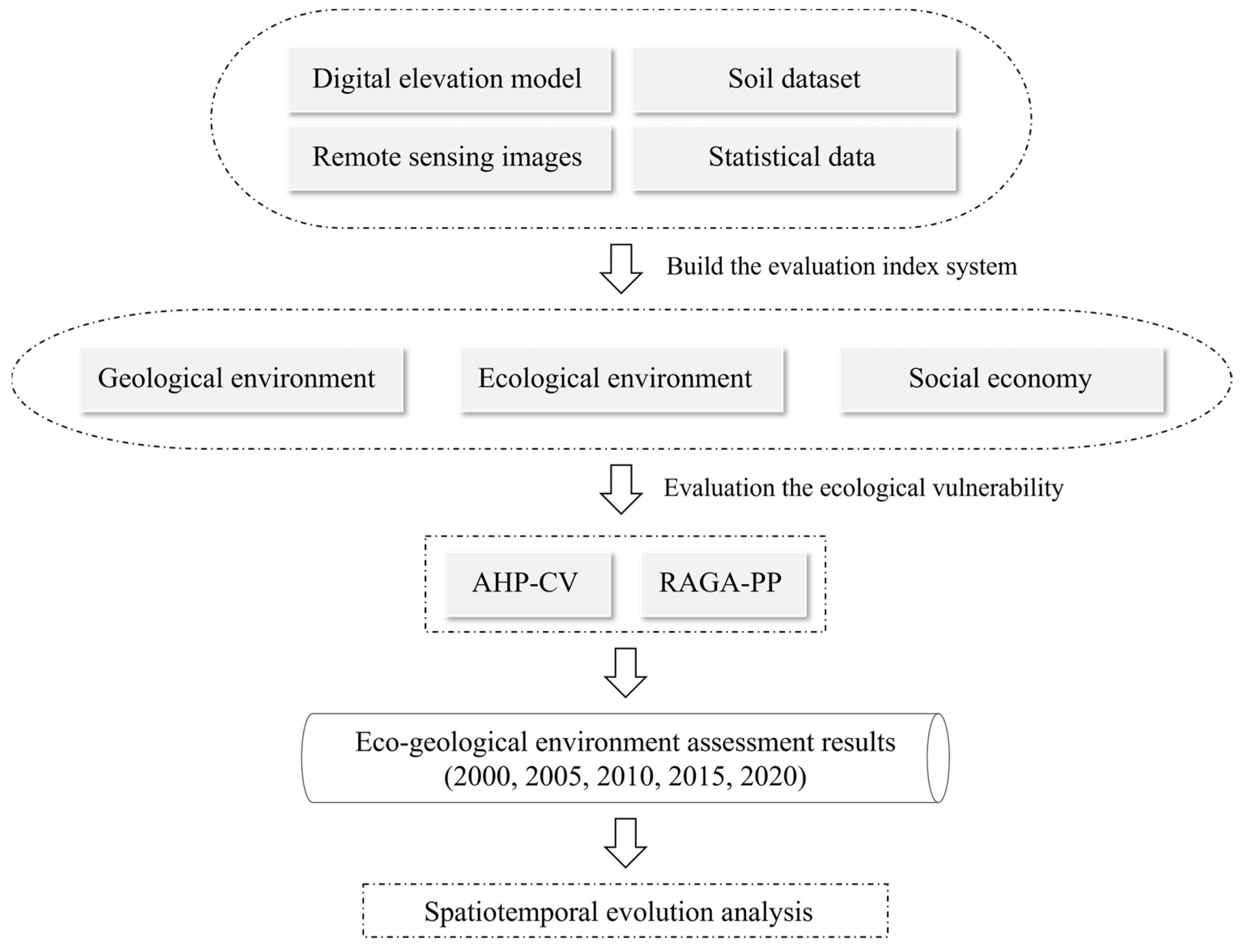
2. Study Area and Data Sources
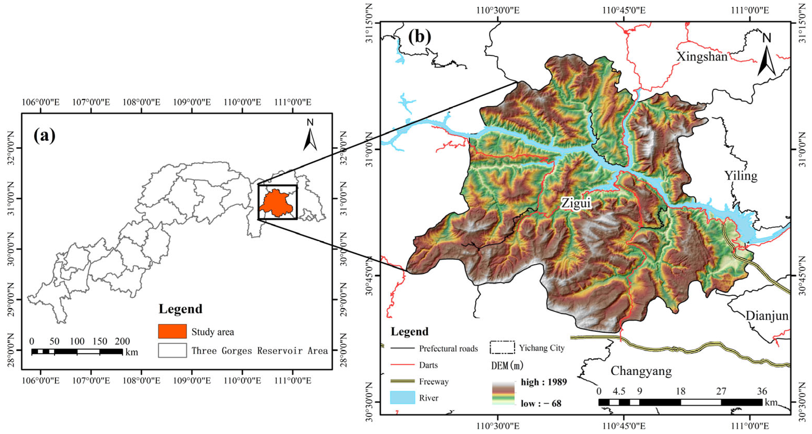
2.1. Study Area
2.2. Data Sources
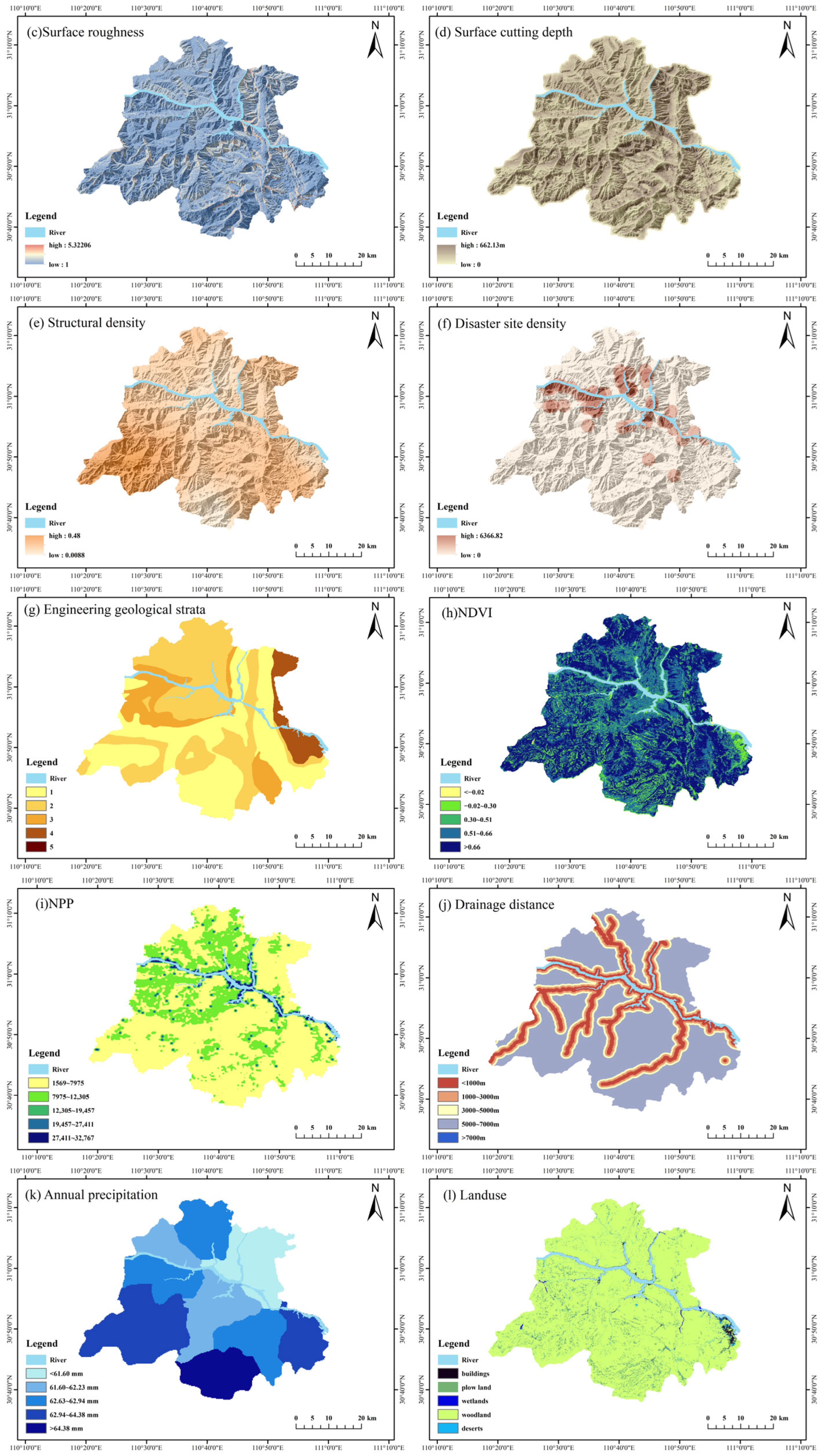
2.3. Selection of Evaluation Factors
- (1)
- Geological environment
- (2)
- Ecological environment
- (3)
- Socioeconomy
3. Methods
3.1. AHP-CV
- (1)
- Construct a judgment matrix
- (2)
- Calculate the relative weight coefficient
- (3)
- Consistency test
- (4)
- Original data collection
- (5)
- Indicator Data Normalization
- (6)
- Data standardization (elimination of scales)
- (7)
- Calculate the CV
- (8)
- Combining the advantages of the subjective assignment AHP method and the objective assignment CV method, the combined weights are obtained through two models for determining the weights in order to make the results more reasonable and accurate:
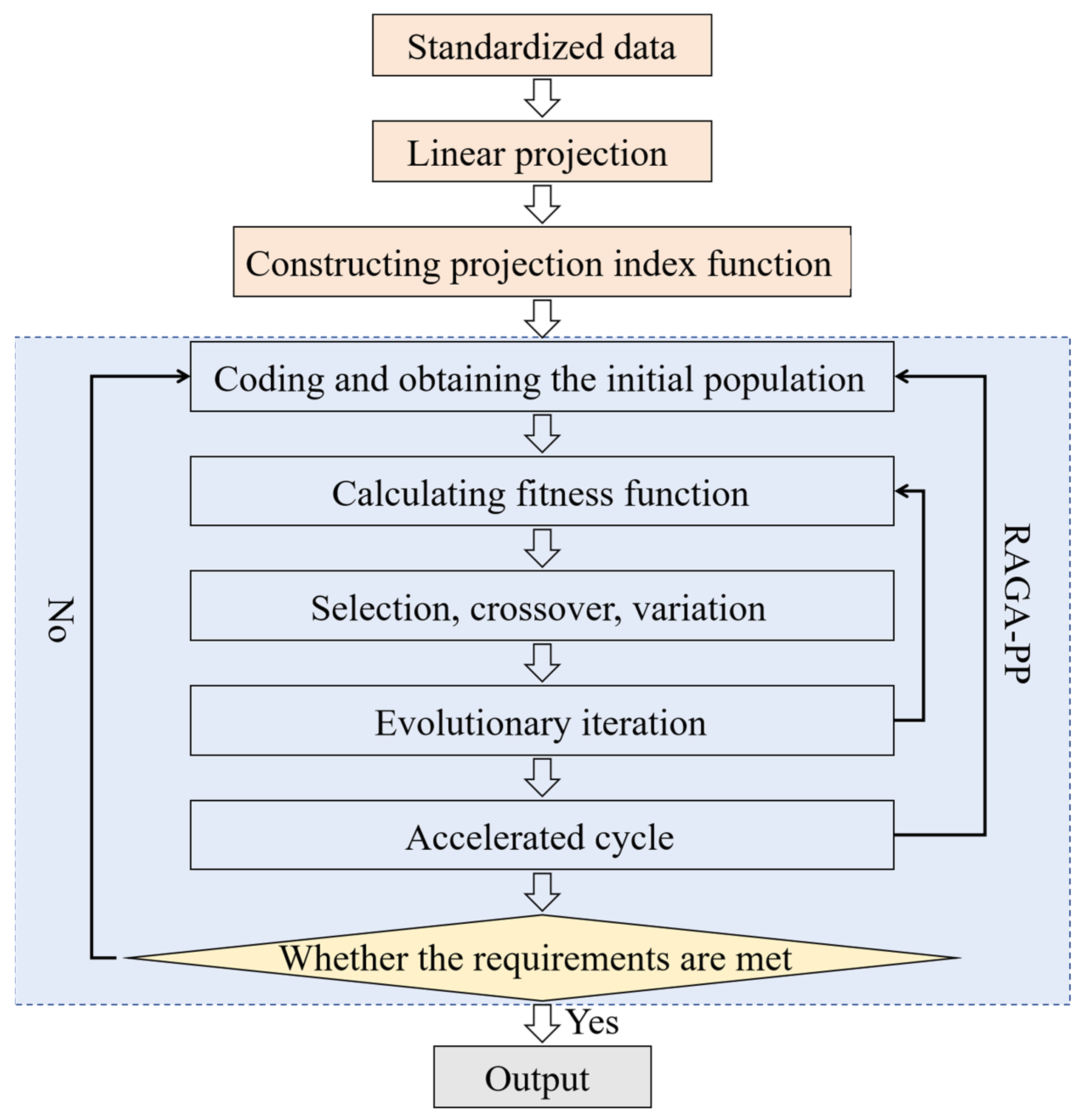
3.2. RAGA-PP
- (1)
- Dimensionless processing
- (2)
- Construct the projection objective function
- (3)
- Optimization of projection index function
4. Results
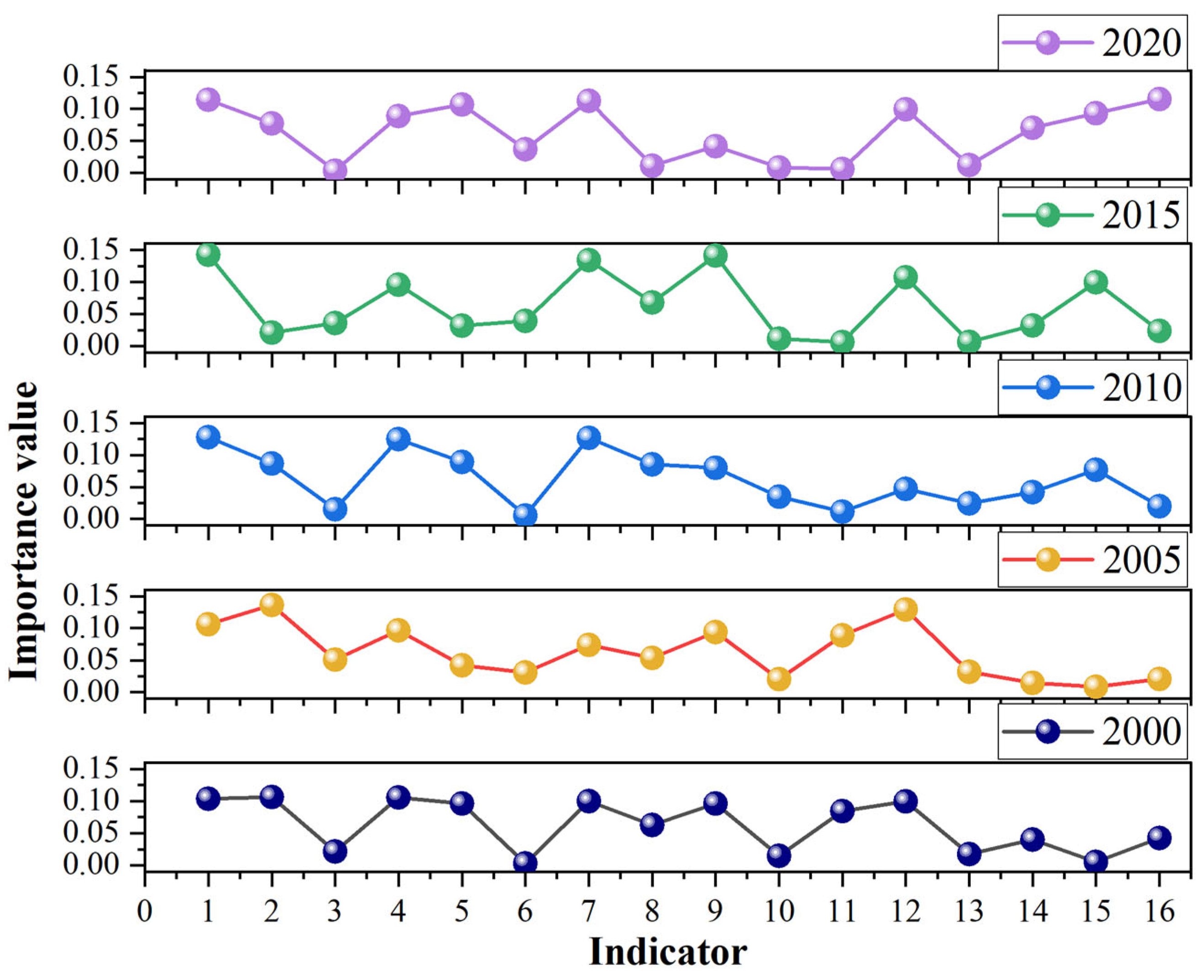
4.1. Eco-Geological Environment Assessment Factors
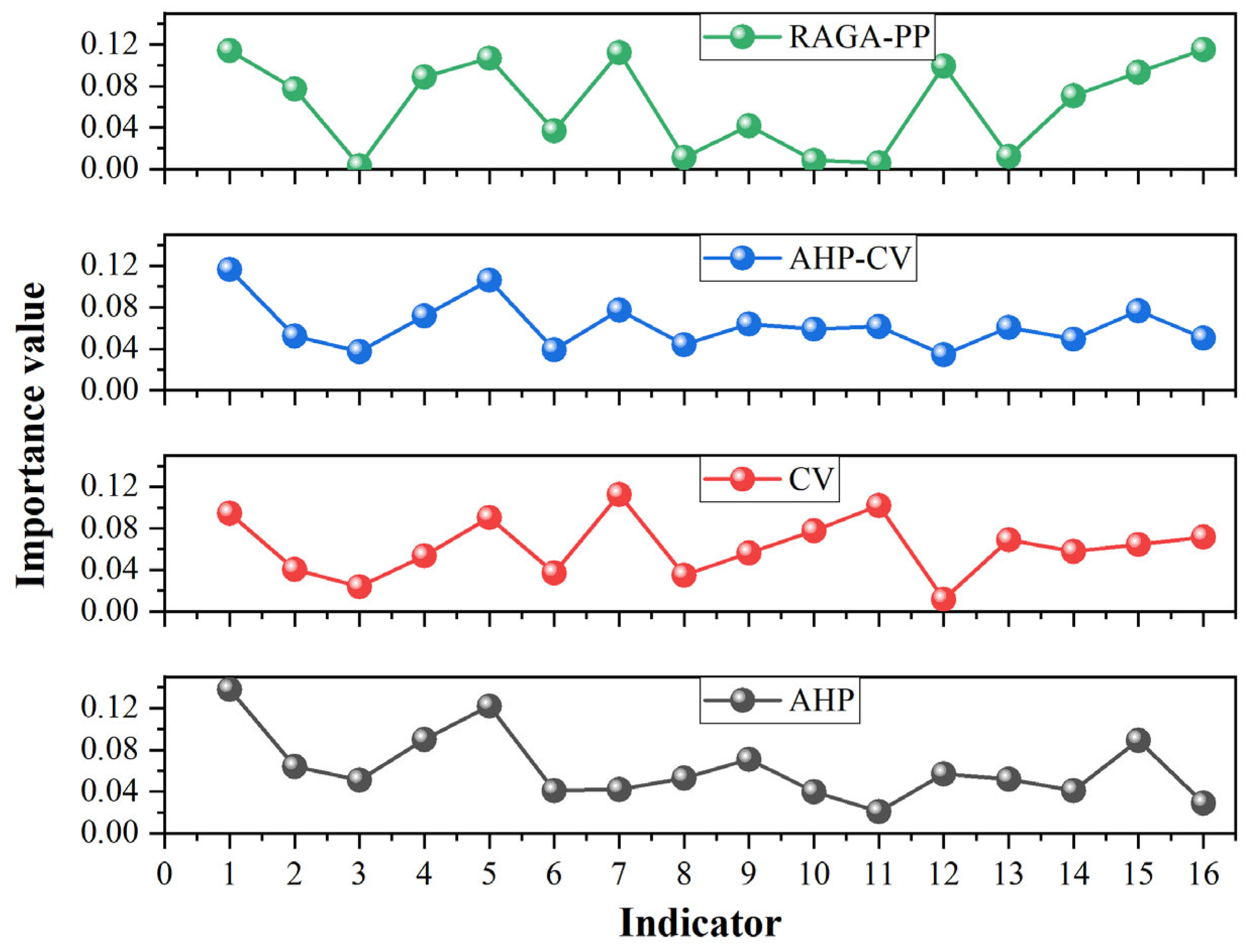
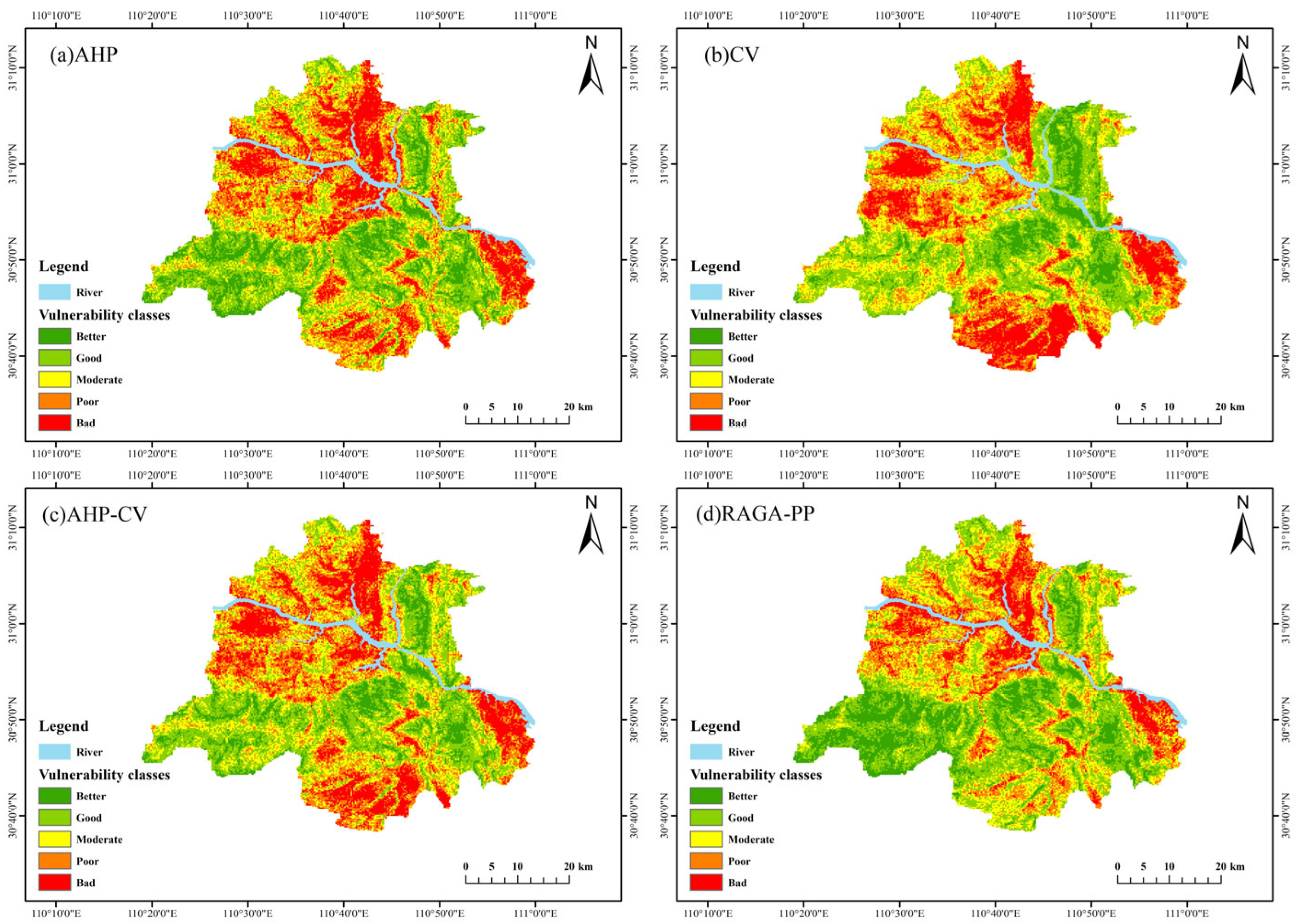
4.2. Eco-Geological Environment Evaluation Results
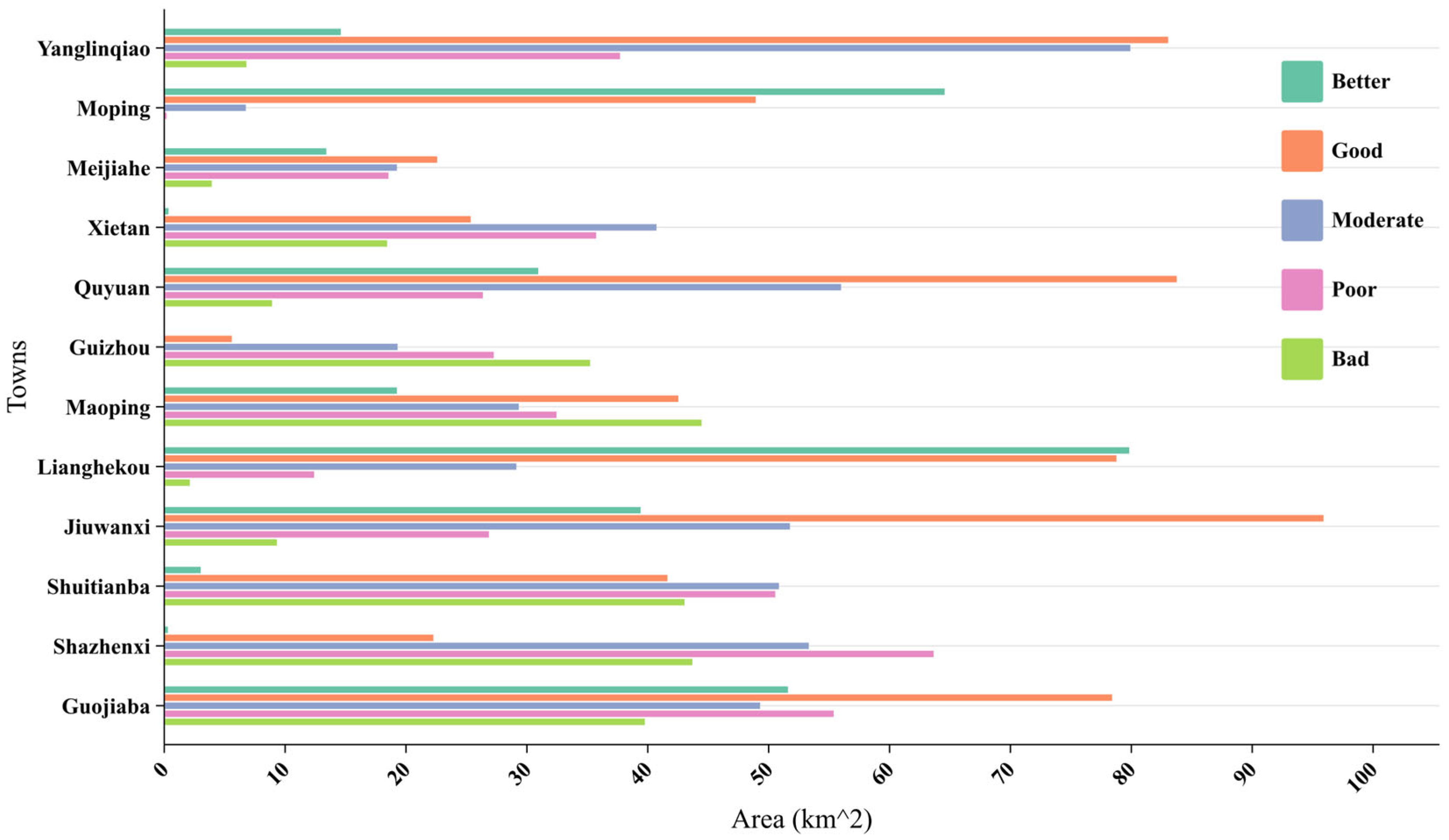
4.3. Eco-Geological Environment of Township Evaluation Results
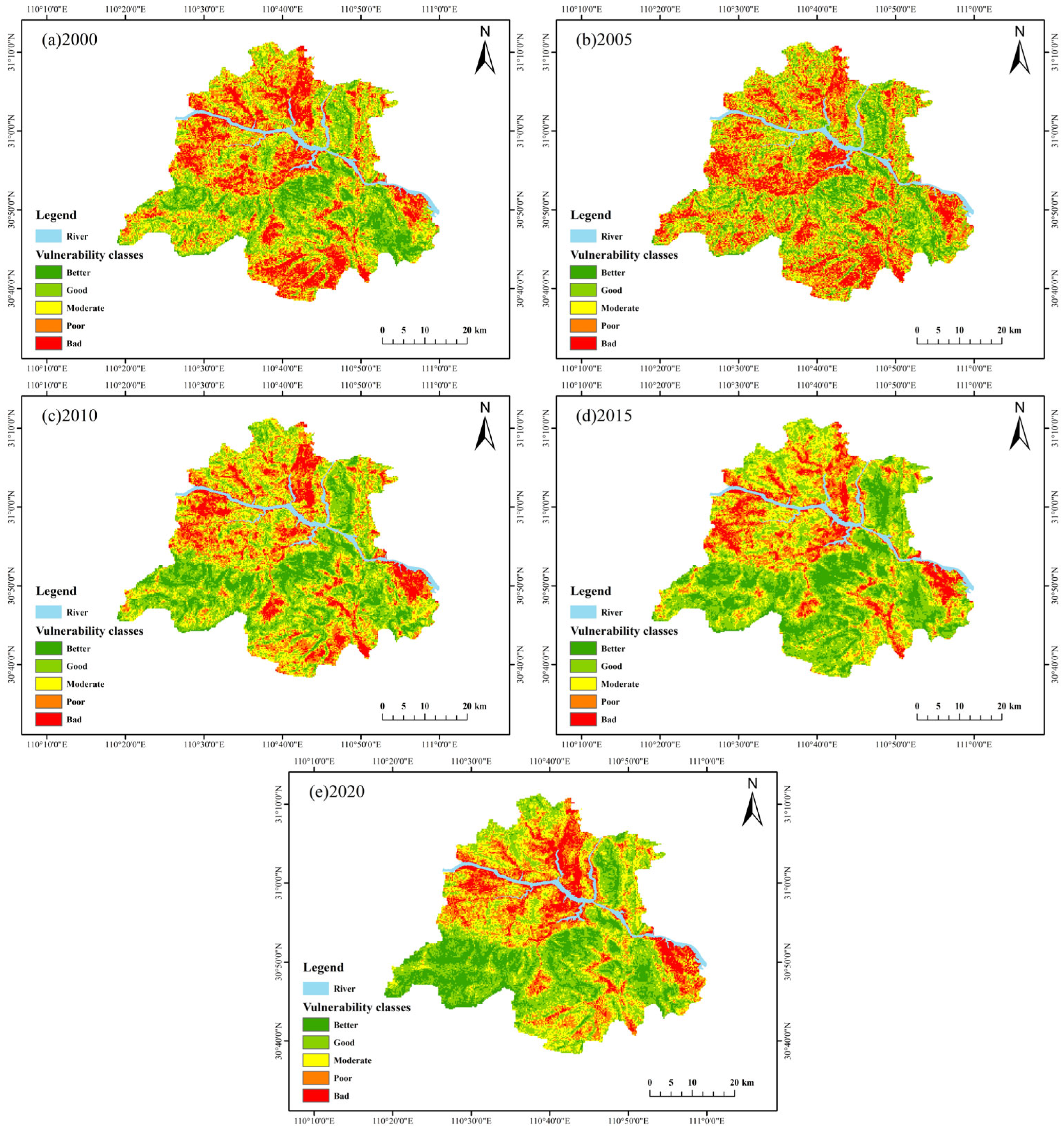
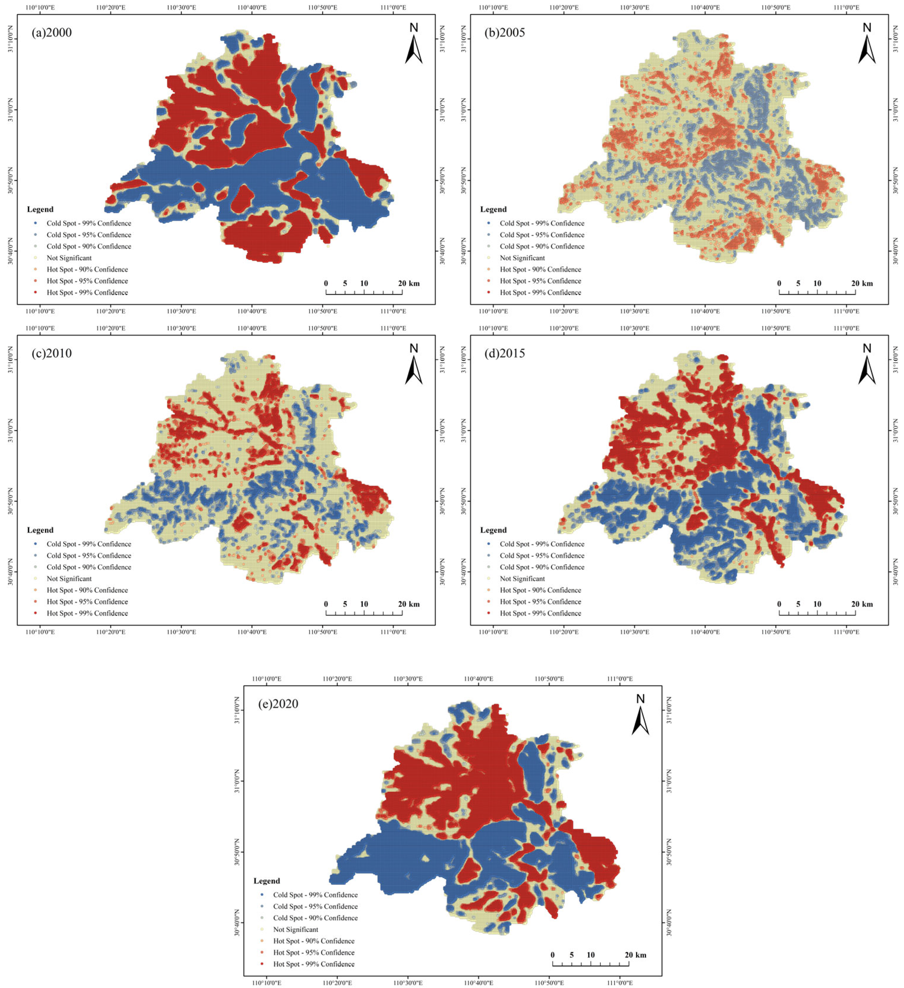
4.4. Spatiotemporal Evolution Results
5. Discussion
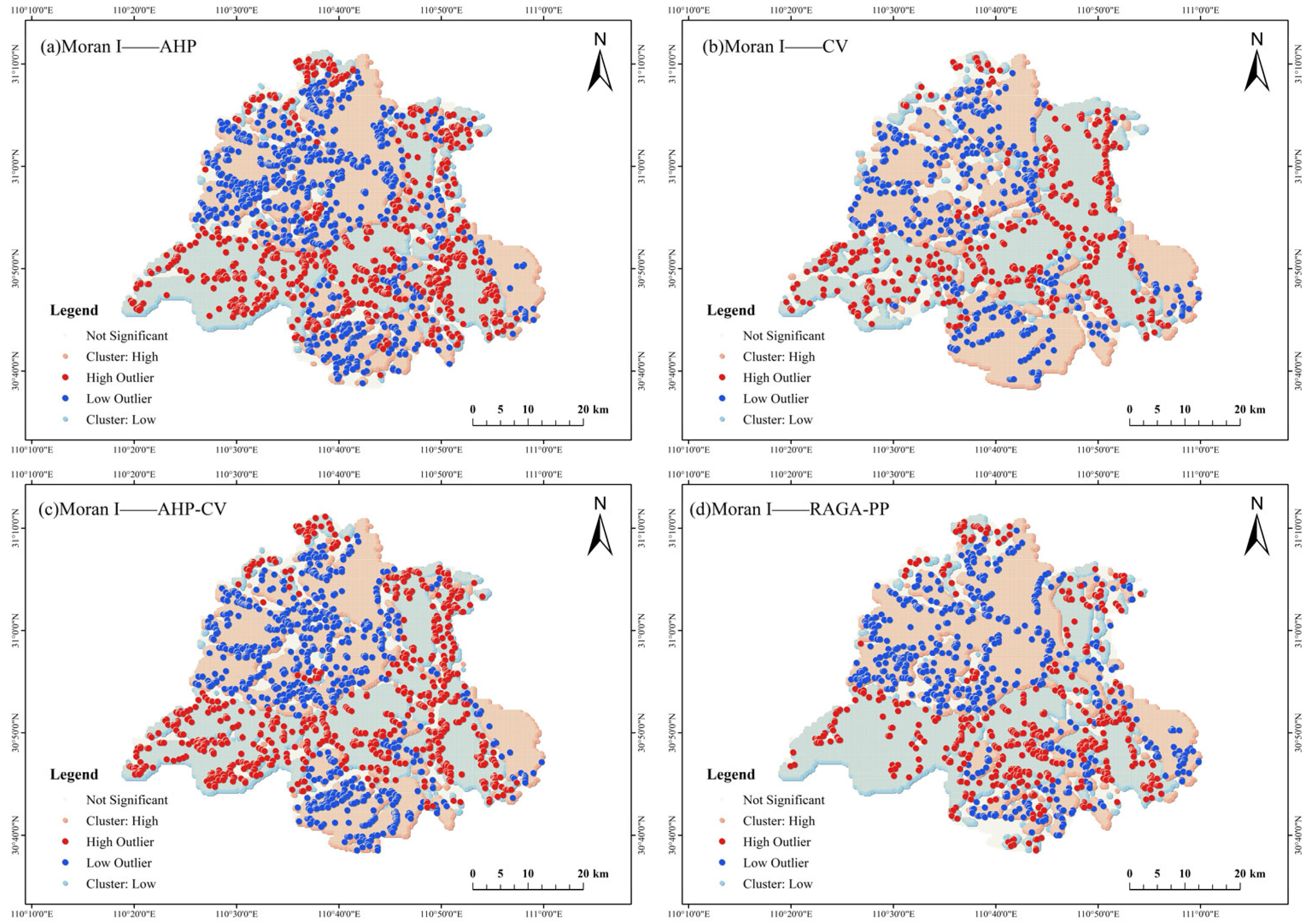
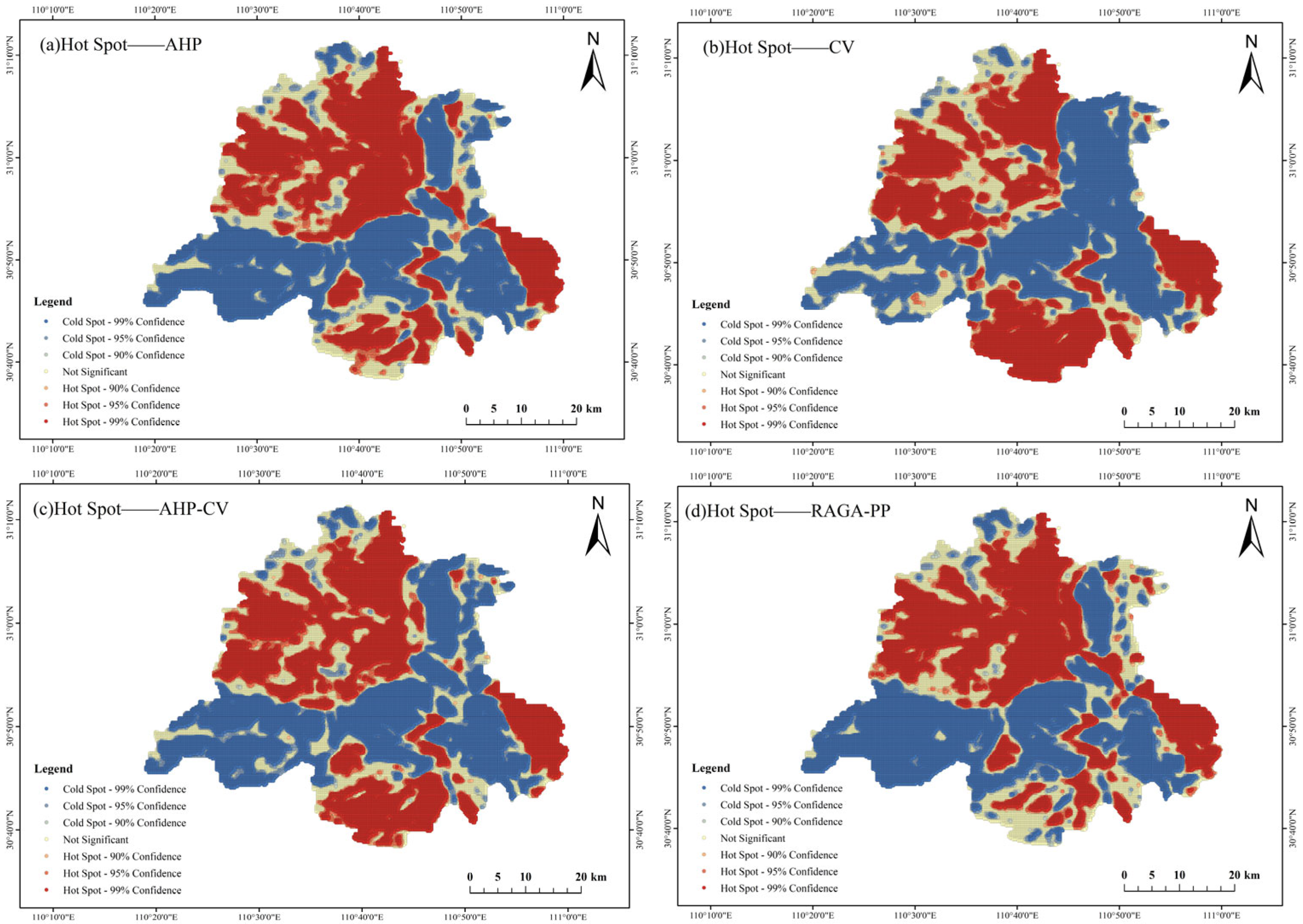
5.1. Spatial Auto-Correlation Analyses
5.2. Hot Spot Analysis
5.3. Eco-Geological Environment Protection and Development Suggestions
6. Conclusions
Author Contributions
Funding
Data Availability Statement
Conflicts of Interest
References
- Chen, X.; Zhu, B.; Liu, Y.; Li, T. Ecological and risk networks: Modeling positive versus negative ecological linkages. Ecol. Indic. 2024, 166, 112362. [Google Scholar] [CrossRef]
- Zhang, X.; Liu, K.; Wang, S.; Wu, T.; Li, X.; Wang, J.; Wang, D.; Zhu, H.; Tan, C.; Ji, Y. Spatiotemporal evolution of ecological vulnerability in the Yellow River Basin under ecological restoration initiatives. Ecol. Indic. 2022, 135, 108586. [Google Scholar] [CrossRef]
- Huang, J.; Zhang, Y.; Zhang, J.; Qi, J.; Liu, P.; Liang, C. Eco-Geological Environment Quality Assessment Based on FAHP-CV Combination Weighting. Sustainability 2023, 15, 10830. [Google Scholar] [CrossRef]
- Zhang, X.; Qiao, W.; Lu, Y.; Sun, F.; Yin, Q. Construction and application of urban water system connectivity evaluation index system based on PSR-AHP-Fuzzy evaluation method coupling. Ecol. Indic. 2023, 153, 110421. [Google Scholar] [CrossRef]
- Yang, W.; Hu, Y.; Ding, D.; Gao, H.; Li, L. Comprehensive Evaluation and Comparative Analysis of the Green Development Level of Provinces in Eastern and Western China. Sustainability 2023, 15, 3965. [Google Scholar] [CrossRef]
- Ahmed, Z.; Zhang, B.; Cary, M. Linking economic globalization economic growth financial development ecological footprint: Evidence from symmetric asymmetric ARDL. Ecol. Indic. 2021, 121, 107060. [Google Scholar] [CrossRef]
- Uehara, T.; Nagase, Y.; Wakeland, W. Integrating Economics and System Dynamics Approaches for Modelling an Ecological-Economic System. Syst. Res. Behav. Sci. 2016, 33, 515–531. [Google Scholar] [CrossRef]
- Zhang, Y.; Shang, K. Evaluation of mine ecological environment based on fuzzy hierarchical analysis and grey relational degree. Environ. Res. 2024, 257, 119370. [Google Scholar] [CrossRef]
- Cui, Y.; Feng, P.; Jin, J.; Liu, L. Water Resources Carrying Capacity Evaluation and Diagnosis Based on Set Pair Analysis and Improved the Entropy Weight Method. Entropy 2018, 20, 359. [Google Scholar] [CrossRef]
- Mei, R. Evaluating the ecological environmental quality of rural tourism using the analytical hierarchy process. Soft Comput. 2024, 28, 3555–3569. [Google Scholar] [CrossRef]
- Newman, K.; King, R.; Elvira, V.; Valpine, P.; McCrea, R.S.; Morgan, B.J.T. State-space models for ecological time-series data: Practical model-fitting. Methods Ecol. Evol. 2023, 14, 26–42. [Google Scholar] [CrossRef]
- Shi, R.; Jia, Q.; Wei, F.; Du, G. Comprehensive evaluation of ecosystem health in pastoral areas of Qinghai-Tibet Plateau based on multi model. Environ. Technol. Innov. 2021, 23, 101552. [Google Scholar] [CrossRef]
- Wu, X.; Zhang, Y. Coupling analysis of ecological environment evaluation and urbanization using projection pursuit model in Xi’an, China. Ecol. Indic. 2023, 156, 111078. [Google Scholar] [CrossRef]
- Ghosh, A.; Maiti, R. Development of new Ecological Susceptibility Index (ESI) for monitoring ecological risk of river corridor using F-AHP and AHP and its application on the Mayurakshi river of Eastern India. Ecol. Inform. 2021, 63, 101318. [Google Scholar] [CrossRef]
- Bai, Z.F.; Han, L.; Liu, H.Q.; Li, L.Z.; Jiang, X.H. Applying the projection pursuit and DPSIR model for evaluation of ecological carrying capacity in Inner Mongolia Autonomous Region, China. Environ. Sci. Pollut. Res. 2024, 31, 3259–3275. [Google Scholar] [CrossRef]
- Saaty, T.L. A scaling method for priorities in hierarchical structures. J. Math. Psychol. 1979, 15, 234–281. [Google Scholar] [CrossRef]
- Niwitpong, S.; Niwitpong, S.A. Confidence intervals for the difference between normal means with known coefficients of variation. Ann. Oper. Res. 2017, 256, 237–251. [Google Scholar] [CrossRef]
- Ji, J.; Chen, J. Urban flood resilience assessment using RAGA-PP and KL-TOPSIS model based on PSR framework: A case study of Jiangsu province, China. Water Sci. Technol. 2022, 86, 3264–3280. [Google Scholar] [CrossRef]
- Gedamu, W.T.; Plank-Wiedenbeck, U.; Wodajo, B.T. A spatial autocorrelation analysis of road traffic crash by severity using Moran’s I spatial statistics: A comparative study of Addis Ababa and Berlin cities. Accid. Anal. Prev. 2024, 200, 107535. [Google Scholar] [CrossRef]
- Chen, L.; Wei, W.; Tong, B.; Chen, L.D. Ecosystem services and their drivers under different watershed- management patterns in the western Chinese Loess Plateau. Ecol. Indic. 2025, 172, 113321. [Google Scholar] [CrossRef]
- Yu, S.; Hou, J.; Lv, J.; Ba, G. Economic benefit assessment of the geo-hazard monitoring and warning engineering system in the Three Gorges Reservoir area: A case study of the landslide in Zigui. Nat. Hazards 2015, 75, S219–S231. [Google Scholar] [CrossRef]

| Data Type | Data Sources | Times |
|---|---|---|
| STRM30 m DEM | http://www.gscloud.cn/ (accessed on 13 March 2023) | 2022 |
| Disaster point data | http://www.yichang.cgs.gov.cn/ (accessed on 13 March 2023) | 2022 |
| Landsat8 data | http://www.gscloud.cn/ (accessed on 13 March 2023) | 2022 |
| Geological maps | http://www.ngac.cn/ (accessed on 15 May 2023) | 2023 |
| Ecological and environmental data | http://ids.ceode.ac.cn/ (accessed on 15 May 2023) | 2023 |
| Social and environmental data | https://www.stats.gov.cn/ (accessed on 23 May 2023) | 2000–2020 |
| Land cover | http://www.globallandcover.com/ (accessed on 23 May 2023) | 2000–2020 |
| Road and river data | https://www.openstreetmap.org/ (accessed on 23 May 2023) | 2000–2020 |
| Factors | Indicators | Number | Types |
|---|---|---|---|
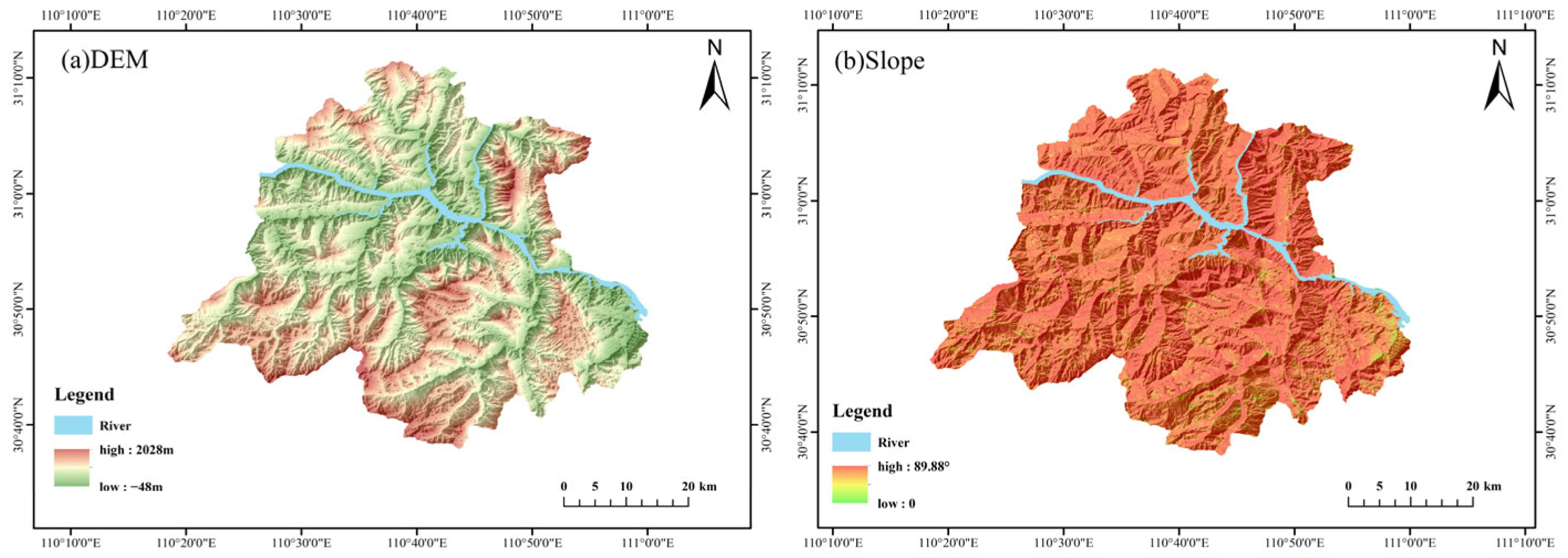
| Geological environment | DEM | 1 | Negative |
| Slope | 2 | Negative | |
| Surface roughness | 3 | Positive | |
| Surface cutting depth | 4 | Negative | |
| Structural density | 5 | Negative | |
| Disaster site density | 6 | Negative | |
| Engineering geological strata | 7 | / | |
| Ecological environment | NDVI | 8 | Positive |
| NPP | 9 | Positive | |
| Drainage distance | 10 | / | |
| Annual precipitation | 11 | Positive | |
| Land-use | 12 | / | |
| Socioeconomy | Road density | 13 | Negative |
| Population density | 14 | Negative | |
| GDP | 15 | Negative | |
| Night-light data | 16 | Negative |
| Indicator | Grading of Evaluation Indicators | ||||
|---|---|---|---|---|---|
| Bad | Poor | Moderate | Good | Better | |
| DEM (m) | ≥1334 | 1022~1334 | 730~1022 | 428~730 | ≤428 |
| Slope (°) | ≥42.84 | 31.67~42.84 | 22.35~31.67 | 13.35~22.35 | ≤13.35 |
| Surface roughness | ≤1.10 | 1.10~1.25 | 1.25~1.49 | 1.49~1.90 | ≥1.90 |
| Surface cutting depth (m) | ≥323.31 | 235.37~323.31 | 168.12~235.37 | 103.46~168.12 | ≤103.46 |
| Structural density (km/km2) | ≥0.35 | 0.26~0.35 | 0.19~0.26 | 0.12~0.19 | ≤0.12 |
| Disaster site density (per/km2) | ≥0.36 | 0.18~0.36 | 0.09~0.18 | 0~0.09 | 0 |
| Engineering geological strata | flexible bulk structure | weak and thinly bedded mud and shale formations | soft—harder thinly bedded moderately thickly laminated sand and mudstone formations | soft and hard medium—thick laminated sandstone and mudstone formations | harder-harder moderately- thickly bedded sandstone plus sandstone groups |
| NDVI | ≤−0.02 | −0.02~0.30 | 0.30~0.51 | 0.51~0.66 | ≥0.66 |
| NPP | 1569~7975 | 7975~12,305 | 12,305~19,457 | 19,457~27,411 | 27,411~32,767 |
| Drainage distance (m) | ≤1000 | 1000~3000 | 3000~5000 | 5000~7000 | ≥7000 |
| Annual precipitation (mm) | ≤61.60 | 61.60~62.23 | 62.23~62.94 | 62.94~64.38 | ≥64.38 |
| Land-use | buildings | plow land | waters, wetlands | woodland, shrubs, grassland | deserts |
| Road density (km/km2) | ≥1.08 | 0.76~1.08 | 0.51~0.76 | 0.31~0.51 | ≤0.31 |
| Population density (per/km2) | ≥2459 | 1176~2459 | 469~1176 | 135~469 | ≤135 |
| GDP per capita (CNY) | ≥437.75 | 245.62~437.75 | 94.63~245.62 | 17.77~94.63 | ≤17.77 |
| Night-light data | ≥31 | 21~31 | 12~21 | 0~12 | 0 |
| Methods | Vulnerability Classes | |||||
|---|---|---|---|---|---|---|
| Better | Good | Moderate | Poor | Bad | ||
| AHP | Area/km2 | 250.31 | 539.43 | 451.04 | 434.86 | 392.02 |
| Proportion/% | 9.72 | 25.55 | 24.76 | 22.67 | 17.31 | |
| CV | Area/km2 | 182.279 | 555.96 | 508.23 | 449.62 | 371.56 |
| Proportion/% | 8.45 | 24.45 | 25.13 | 23.75 | 18.21 | |
| AHP-CV | Area/km2 | 193.11 | 540.64 | 486.31 | 462.73 | 384.87 |
| Proportion/% | 12.72 | 29.29 | 26.19 | 19.82 | 11.97 | |
| RAGA-PP | Area/km2 | 317.14 | 629.49 | 479.16 | 386.88 | 255.00 |
| Proportion/% | 15.34 | 30.44 | 23.17 | 18.71 | 12.33 | |
| Townships | Better | Good | Moderate | Poor | Bad |
|---|---|---|---|---|---|
| Area/km2 | Area/km2 | Area/km2 | Area/km2 | Area/km2 | |
| Yanglinqiao | 14.61 | 83.05 | 79.92 | 37.70 | 6.80 |
| Moping | 64.56 | 48.93 | 6.75 | 0.20 | 0.00 |
| Meijiahe | 13.41 | 22.58 | 19.25 | 18.55 | 3.93 |
| Xietan | 0.35 | 25.35 | 40.72 | 35.73 | 18.44 |
| Quyuan | 30.94 | 83.76 | 55.99 | 26.36 | 8.92 |
| Guizhou | 0.00 | 5.59 | 19.30 | 27.26 | 35.23 |
| Maoping | 19.25 | 42.53 | 29.33 | 32.45 | 44.45 |
| Lianghekou | 79.83 | 78.77 | 29.13 | 12.40 | 2.12 |
| Jiuwanxi | 39.41 | 95.90 | 51.76 | 26.86 | 9.32 |
| Shuitianba | 3.02 | 41.63 | 50.85 | 50.55 | 43.04 |
| Shazhenxi | 0.30 | 22.27 | 53.32 | 63.65 | 43.69 |
| Guojiaba | 51.60 | 78.41 | 49.29 | 55.38 | 39.76 |
| Methods | Vulnerability Classes | |||||
|---|---|---|---|---|---|---|
| Better | Good | Moderate | Poor | Bad | ||
| 2000 | Area/km2 | 199.01 | 523.40 | 507.13 | 464.29 | 354.53 |
| Proportion/% | 9.72 | 25.55 | 24.76 | 22.67 | 17.31 | |
| 2005 | Area/km2 | 174.17 | 503.75 | 517.71 | 489.24 | 375.14 |
| Proportion/% | 8.45 | 24.45 | 25.13 | 23.75 | 18.21 | |
| 2010 | Area/km2 | 260.99 | 601.01 | 537.36 | 406.74 | 245.68 |
| Proportion/% | 12.72 | 29.29 | 26.19 | 19.82 | 11.97 | |
| 2015 | Area/km2 | 329.53 | 671.21 | 499.21 | 348.68 | 205.76 |
| Proportion/% | 16.04 | 32.67 | 24.30 | 16.97 | 10.02 | |
| 2020 | Area/km2 | 317.14 | 629.49 | 479.16 | 386.88 | 255.00 |
| Proportion/% | 15.34 | 30.44 | 23.17 | 18.71 | 12.33 | |
| Moran I | z | p | |
|---|---|---|---|
| AHP | 0.776 | 522.71 | 0.00 |
| CV | 0.841 | 566.46 | 0.00 |
| AHP-CV | 0.792 | 533.80 | 0.00 |
| RAGA-PP | 0.815 | 548.78 | 0.00 |
Disclaimer/Publisher’s Note: The statements, opinions and data contained in all publications are solely those of the individual author(s) and contributor(s) and not of MDPI and/or the editor(s). MDPI and/or the editor(s) disclaim responsibility for any injury to people or property resulting from any ideas, methods, instructions or products referred to in the content. |
© 2025 by the authors. Licensee MDPI, Basel, Switzerland. This article is an open access article distributed under the terms and conditions of the Creative Commons Attribution (CC BY) license (https://creativecommons.org/licenses/by/4.0/).
Share and Cite
Wu, X.; Lu, J.; Lv, C.; Qin, L.; Liu, R.; Zheng, Y. Spatiotemporal Analysis of Eco-Geological Environment Using the RAGA-PP Model in Zigui County, China. Remote Sens. 2025, 17, 2414. https://doi.org/10.3390/rs17142414
Wu X, Lu J, Lv C, Qin L, Liu R, Zheng Y. Spatiotemporal Analysis of Eco-Geological Environment Using the RAGA-PP Model in Zigui County, China. Remote Sensing. 2025; 17(14):2414. https://doi.org/10.3390/rs17142414
Chicago/Turabian StyleWu, Xueling, Jiaxin Lu, Chaojie Lv, Liuting Qin, Rongrui Liu, and Yanjuan Zheng. 2025. "Spatiotemporal Analysis of Eco-Geological Environment Using the RAGA-PP Model in Zigui County, China" Remote Sensing 17, no. 14: 2414. https://doi.org/10.3390/rs17142414
APA StyleWu, X., Lu, J., Lv, C., Qin, L., Liu, R., & Zheng, Y. (2025). Spatiotemporal Analysis of Eco-Geological Environment Using the RAGA-PP Model in Zigui County, China. Remote Sensing, 17(14), 2414. https://doi.org/10.3390/rs17142414