Hybrid GIS-Transformer Approach for Forecasting Sentinel-1 Displacement Time Series

Abstract

This study presents a deep learning-based approach for forecasting Sentinel-1 displacement time series, with particular attention to irregular temporal patterns—an aspect often overlooked in previous works. Displacement data were generated using the Parallel Small BAseline Subset (P-SBAS) technique via the Geohazard Thematic Exploitation Platform (G-TEP). Initial experiments on a regular dataset from Lombardy employed Long Short-Term Memory (LSTM) models to forecast multiple future time steps. Empirical analysis determined that optimal forecasting is achieved with a 50-time-step input sequence, and that predicting 10% of the input sequence length strikes a balance between temporal coverage and accuracy. The investigation then extended to irregular datasets from Lisbon and Washington, comparing two preprocessing strategies: imputation and the inclusion of time intervals as a second feature. While imputation improved one-step predictions, it was inadequate for multi-step forecasting. To address this, a Time-Gated LSTM (TG-LSTM) was implemented. TG-LSTM outperformed standard LSTM for irregular data in one-step prediction but faced limitations in handling heteroscedasticity and computational cost during multi-step forecasting. These issues were effectively resolved using Temporal Fusion Transformers (TFT), which achieved the best performance, with RMSE values of 1.71 mm/year (Lisbon) and 1.26 mm/year (Washington). A key contribution of this work is the development of a GIS-integrated forecasting toolbox that incorporates LSTM models for regular sequences and TG-LSTM/TFT models for irregular ones. The toolbox enables both single- and multi-step displacement predictions, offering a scalable solution for geohazard monitoring and early warning applications.

1. Introduction

Predicting displacements in time series is critical for a comprehensive understanding of ground movements and their broader implications [1]. Such predictions play a pivotal role in disaster management, environmental monitoring, infrastructure maintenance, resource management, and public safety, ultimately contributing to informed decision-making, risk mitigation, and sustainable development [2,3].

Despite its significance, displacement time series forecasting remains inherently complex, requiring a holistic approach that considers data quality, appropriate model selection, and a nuanced understanding of underlying temporal patterns [4,5]. Among these patterns, trends and seasonality are fundamental elements shaping time series behavior [6]. Trends reflect long-term directional movements—whether increasing, decreasing, or stabilizing—while seasonality captures periodic fluctuations occurring at regular intervals, such as daily, weekly, or monthly cycles, as illustrated in Figure 2 of [7]. Properly identifying these components is essential for enhancing predictive accuracy.

Beyond trends and seasonality, several additional challenges complicate displacement forecasting. High dimensionality, characterized by numerous features, can hinder precise modeling and substantially increase computational demands [8,9]. Noise and outliers, as illustrated in Figure 4 of [10], can obscure meaningful patterns and degrade model performance. Moreover, non-stationarity—where statistical properties such as mean and variance evolve over time—introduces instability into predictive models, as shown in Figure 2.3 of [11].

Among these challenges, irregular sampling emerges as a particularly critical obstacle to displacement monitoring, which severely undermines the effectiveness of standard forecast techniques. Addressing irregularity is thus essential for advancing reliable displacement predictions. Irregular sampling complicates modeling efforts by introducing non-uniform temporal structures that hinder accurate pattern recognition and learning. A comprehensive review [12] highlights two principal strategies for managing such irregular data: imputing missing values prior to model training or modifying Recurrent Neural Networks (RNNs) to handle variable intervals natively. Other studies have explored diverse approaches, including correlation analysis methods for irregular series [13], penalization strategies for irregular periodicities [14], specialized architectures such as the Dual-Attention Time-Aware Gated Recurrent Unit (DATA-GRU) [15] and neural-controlled differential equation models [16]. These contributions collectively underscore the increasing recognition of irregular sampling as a major barrier in time series forecasting, motivating the development of specialized methodologies, particularly in the context of geohazard monitoring.

To understand the motivation behind recent deep learning-based forecasting models, it is essential to consider how classical time series methods have traditionally addressed displacement modeling challenges. Classical time series forecasting methods provide a structured foundation for analyzing temporal data. AutoRegressive (AR) models predict future values as linear combinations of past observations, making them suitable for stationary series exhibiting autocorrelation [17]. Moving Average (MA) models represent current values based on past forecast errors, effectively capturing short-term fluctuations but also requiring stationarity [18]. The AutoRegressive Moving Average (ARMA) model combines AR and MA components to better capture both the systematic patterns and residual noise in stationary data [19]. To address non-stationarity due to trends, AutoRegressive Integrated Moving Average (ARIMA) models introduce differencing, transforming the data into a stationary form and enabling broader applicability to non-seasonal datasets with trends [17]. When seasonality is present, the Seasonal AutoRegressive Integrated Moving Average (SARIMA) model extends ARIMA by incorporating seasonal autoregressive and moving-average components, allowing it to capture both trend and seasonal patterns. However, Long Short-Term Memory (LSTM) models have demonstrated superior performance in such contexts, as shown in [20]. The Seasonal Autoregressive Integrated Moving Average Exogenous (SARIMAX) model incorporates seasonal and exogenous variables to enhance accuracy, particularly for datasets with aligned input–output lengths [21]. While SARIMA captures both trend and seasonal components and SARIMAX enhances accuracy with exogenous variables, these classical models are limited in handling nonlinearities and long-term dependencies. Long Short-Term Memory (LSTM) networks address these challenges by modeling complex temporal dynamics more effectively [22].

Outside the ARIMA family, Exponential Smoothing methods use exponentially weighted averages of past observations, providing adaptive forecasts for level changes; however, basic forms exclude trend or seasonality, which are addressed by Double and Triple Exponential Smoothing (Holt–Winters). The Holt–Winters method addresses these limitations by incorporating separate smoothing equations for level, trend, and seasonality, making it well-suited for structured seasonal data [23].

Recent studies in InSAR time series forecasting with Sentinel-1 data further contextualize this research. Traditional statistical models such as SARIMA and sinusoidal extrapolation have proven effective for short- and long-term forecasts, respectively, but struggle with non-stationary signals and irregular seasonal patterns [24]. Machine learning approaches have expanded this landscape: Fiorentini et al. [25] applied Support Vector Machines and Boosted Regression Trees for road displacement prediction, while Radman et al. [26] introduced ensemble DL models combining Multi-Layer Perceptron (MLP), Convolutional Neural Networks (CNNs), and LSTM for subsidence forecasting. Although promising, these approaches were often limited by data sparsity, coherence loss, and resolution mismatches. LSTM-based methods, such as those by Abdikan et al. [27] and Mirmazloumi et al. [28], showed improvements in forecasting and anomaly detection but remained vulnerable to reduced spatial granularity, noise, and seasonal insensitivity. To address irregular sampling, Lattari et al. [29] proposed the TG-LSTM, which improved adaptability but struggled with capturing seasonal behaviors. More recently, Transformer-based architectures have gained traction: Wang et al. [30] applied self-attention mechanisms for permafrost monitoring, achieving enhanced feature representation, while Wang et al. [31] further developed Spacetimeformer for spatiotemporal forecasting, though it remained heavily dependent on time-series deformation maps and required substantial preprocessing. Complementary studies, such as Gualandi et al. [32], employed Variational Bayesian Independent Component Analysis (vbICA) to isolate deformation sources, yet faced challenges related to stability and sensitivity to initialization.

Collectively, these contributions reflect a growing movement towards integrating data-driven models for complex displacement forecasting. However, persistent challenges remain, particularly in managing irregular sampling, capturing long-term trends, and balancing computational efficiency with predictive accuracy. These challenges form the core motivation behind our proposed approach, which explicitly addresses irregular sampling, supports multi-step forecasting, and embeds the methodology within a GIS-integrated framework for scalable, context-aware geohazard monitoring.

To address these unmet needs, our study begins by systematically evaluating forecasting techniques on displacement time series with regular temporal sampling. Specifically, a regular dataset from Lombardy was analyzed using LSTM models to predict multiple future time steps. Empirical evaluation revealed that the forecast accuracy diminishes as the prediction horizon extends. This finding emphasizes the importance of carefully selecting the number of future steps to maintain model reliability and establishes a benchmark for subsequent experiments.

Building on these insights, the study transitions to forecasting irregular displacement time series from Lisbon and Washington. Within the standard LSTM framework, two key approaches were explored: imputing missing values and integrating time intervals as a second feature. Although imputation improved single-step prediction, standard LSTM models struggled with multi-step forecasting in irregular contexts. To address these limitations, a Time-Gated LSTM (TG-LSTM) architecture was implemented, incorporating time intervals directly into the modeling process. TG-LSTM demonstrated improved adaptability to irregular temporal structures but continued to exhibit limitations related to heteroscedasticity and computational cost. Further advancements were achieved with the implementation of the Temporal Fusion Transformer (TFT) model, which successfully reduced computational burdens and better managed heteroscedasticity patterns. By integrating attention mechanisms and gating strategies, TFT outperformed traditional recurrent models in both predictive accuracy and interpretability, establishing itself as a robust architecture for displacement forecasting.

Moreover, this work emphasizes the potential of integrating Deep Learning (DL), Interferometric Synthetic Aperture Radar (InSAR), and Geographic Information Systems (GIS) for comprehensive geospatial analysis. This interdisciplinary integration offers a new perspective on Earth’s surface dynamics by leveraging GIS for spatial data analysis, DL for advanced temporal modeling, and InSAR for high-precision surface movement measurements. However, a noticeable gap persists: the lack of comprehensive toolboxes that combine GIS, AI, and InSAR technologies within widely used platforms such as ArcGIS Pro. This gap particularly affects users with limited expertise or resources to develop such integrative tools.

To bridge this gap, we developed a specialized GIS-integrated toolbox that enables single- and multi-step displacement forecasting within a spatial analysis environment. This toolbox democratizes access to advanced forecasting capabilities, allowing both expert and non-expert users to leverage state-of-the-art DL methodologies for Earth surface monitoring.

The novelty of this research lies in its end-to-end exploration of forecasting both regular and irregular Sentinel-1 displacement time series using advanced DL architectures. Unlike prior studies that typically focus on either regular datasets or isolated modeling strategies, this work systematically evaluates multiple approaches—including missing value imputation, time interval embedding, Time-Gated LSTM, and Temporal Fusion Transformers—across varying temporal structures. A key contribution is the demonstration that TFT outperforms traditional LSTM-based methods in the multi-step forecasting of irregular time series, effectively mitigating challenges related to heteroscedasticity and computational cost. Additionally, the study presents a novel GIS-integrated toolbox that operationalizes the best-performing models, thereby enhancing the practical usability of DL methods in geospatial science.

2. InSAR Time Series Generation and Preprocessing Strategy

2.1. The Geohazard Thematic Exploitation Platform (G-TEP)

The displacement time series used in this study were generated via the P-SBAS service available on the G-TEP [33]. It offers scalable access to a wide range of satellite datasets, including both optical and Synthetic Aperture Radar (SAR) imagery, along with advanced processing capabilities through user-configurable and modular workflows.

In this study, G-TEP was instrumental in generating the displacement time series that served as the primary input for our analysis. Through the processing of complete Sentinel-1 Interferometric Wide-Swath (IW) Single-Look Complex (SLC) image stacks, the platform produced validated, geocoded Line-of-Sight (LoS) displacement time series—forming a robust foundation for the time-series decomposition and predictive modeling tasks that followed.

2.2. Parallel Small BAseline Subset (P-SBAS) Processing

The P-SBAS methodology, as implemented on G-TEP, represents a significant advancement of the traditional Small BAseline Subset (SBAS) technique. By integrating high-performance computing resources and fine-grained parallelization strategies, it addresses key computational bottlenecks commonly encountered in SBAS workflows—such as interferogram generation, phase unwrapping, time series inversion, and Atmospheric Phase Screen (APS) correction. Leveraging a distributed cloud infrastructure, P-SBAS significantly accelerates processing times, making it well-suited for near-real-time displacement monitoring in support of early warning systems and rapid response applications [34].

The full P-SBAS processing chain on G-TEP [35] ensures consistency and reproducibility in large-scale interferometric analyses. In the standard P-SBAS processing chain, the final displacement products are typically refined to a spatial resolution of approximately 26 × 30 m—an optimized balance aimed at maximizing the signal-to-noise ratio (SNR) while retaining adequate spatial detail for interpreting ground deformation. This resolution is achieved by applying 20 looks in range and 5 in azimuth during multilooking, a process that improves the SNR by averaging uncorrelated phase contributions and mitigating decorrelation effects. The geocoded products are then resampled based on the 1-arcsecond SRTM DEM, yielding a pixel spacing consistent with the 30 m grid seen in the output GeoTIFFs.

2.3. Preprocessing and Datasets

Before initiating the preprocessing of the available displacement time series datasets, it is essential to conduct an analytical examination of their fundamental components. This includes assessing the trend, stationarity, and seasonality patterns inherent in each dataset. The initial analytical framework employed in this study was not designed to accommodate the irregular time series data from the Lisbon and Washington datasets. In contrast, the Lombardy dataset exhibited a regular time series structure, making it more suitable for this analytical approach. Consequently, the displacement time series data from Lisbon and Washington were resampled and transformed into regular datasets prior to the analysis of their time series components.

In the provided Figure 1, Figure 2 and Figure 3 the trend, seasonal, and residual components of time series samples from the Lombardy, Lisbon, and Washington datasets were extracted using the UnobservedComponents class from the statsmodels.tsa.statespace.structural module in Python [36]. This model implements the Unobserved Components Model (UCM) [37,38], a flexible probabilistic framework for time series decomposition that represents the observed series $y_t$ as the sum of latent stochastic processes:

$$y_t=T_t+S_t+R_t,$$

where $T_t$ denotes the trend component, $S_t$ captures the seasonal variation, and $R_t$ accounts for the residual or irregular fluctuations.

Unlike classical decomposition techniques that rely on deterministic smoothing, the UCM approach models each component as an evolving stochastic process, estimating their dynamics via maximum likelihood within a state-space formulation. In this study, the trend was specified as a local linear trend, permitting both the level and the slope to vary over time, thereby capturing gradual changes in ground displacement. The seasonal component was modeled with a periodicity of twelve months to reflect expected intra-annual variations, consistent with the typical revisit interval of Sentinel-1 acquisitions and the physical phenomena influencing displacement patterns. The residual component encapsulates short-term variations not explained by the trend or seasonality.

This decomposition method offers enhanced flexibility compared to traditional approaches, as it allows for nonstationary behavior in both the trend and seasonal components.

The results revealed limited or no long-term trends but a clear seasonal component across the datasets, offering valuable insights for modeling and forecasting ground displacements.

It is important to note that the presence of strong seasonal fluctuations does not pose a significant challenge for LSTM models. LSTMs are well-suited for capturing and learning from such periodic patterns due to their ability to recognize and retain long-term dependencies in sequential data.

The primary preprocessing methods employed included the imputation of missing values and feature engineering. Specifically, backward filling was used for imputation due to its simplicity and effectiveness in handling moderate data irregularities, as observed in the Washington and Lisbon datasets. Additionally, feature engineering was applied by embedding time as a second feature to enrich the datasets.

In the Lisbon dataset, the primary time interval observed was 6 days, with occasional irregular intervals of 12, 18, and 24 days. In the Washington dataset, the first two intervals—48 and 222 days—were significantly longer than the typical 12-day spacing. These two data points were excluded prior to backward filling to prevent bias and ensure the reliability of the imputed values.

The preprocessing methods were based on the following principles:

• Missing Values Imputation (Backward Filling): This method replaces a missing value at time t with the observation at time $t+1$. It is effective for short gaps or when later values are more representative. Figure 4 illustrates the application of this method on synthetic displacement data with 15% missing values. This imputation technique regularizes the time series by filling gaps, allowing it to be used as input for models that require uniform time intervals, such as standard LSTMs. It should be noted that missing values were imputed on the basis of the minimum observed temporal interval in the dataset to maintain temporal consistency.
• Feature Engineering (Embedding Time Intervals): Intervals between observations were embedded as a second feature. Instead of using a univariate displacement sequence, the input was structured as a multivariate time series (sequence length, 2) consisting of displacement and time interval. This structure enhances the model’s awareness of irregular measurement spacing and improves its ability to capture dynamics influenced by temporal gaps [39].

The following subsections provide a description of each dataset used.

2.3.1. Lombardy Dataset

Lombardy is one of the most seismically and landslide-active regions in northern Italy [40]. The region exhibits significant geomorphological diversity [41], with mountainous terrain covering approximately 40.5% of its area. According to the Italian National Institute for Environmental Protection and Research (ISPRA) [42], provinces such as Sondrio, Bergamo, Lecco, Brescia, and Como show high to very high landslide susceptibility. Moreover, Lombardy has experienced intense land use and urban development, often in geologically unstable zones, exacerbating its vulnerability to ground deformation. The time frame considered in our analysis encompasses a major hydrogeological event that occurred on 26–27 July 2021, which severely impacted towns around Lake Como—triggering numerous landslides, damaging infrastructure, and highlighting the necessity for displacement monitoring in such dynamic environments.

Table 1. Summary of key parameters extracted from the P-SBAS analysis of the Lombardy dataset. The corresponding geographic location is shown in Appendix A (Figure A1).

Dataset	Start Date	End Date	NoI	DEM	Coh.	BBX	Orb.
Lombardy (Italy)	7 January 2020	17 August 2021	50	SRTM1 arcsec	0.85	44.943°, 8.693° 46.884°, 12.231°	Desc.

presents the selected parameters used in the P-SBAS analysis for the Lombardy dataset, including the start and end dates, number of images (NoI), DEM, temporal coherence (Coh.), bounding box (BBX), and orbit direction (Orb.). The same parameters are also reported for the Lisbon and Washington datasets in

Table 2. Summary of key parameters extracted from the P-SBAS analysis of the Lisbon dataset. The corresponding geographic location is shown in Appendix A (Figure A2).

Dataset	Start Date	End Date	NoI	DEM	Coh.	BBX	Orb.
Lisbon (Portugal)	26 January 2018	27 April 2020	50	SRTM1 arcsec	0.6	38.088°, −11.124° 39.800°, −7.945°	Asc.

and

Table 3. Summary of key parameters extracted from the P-SBAS analysis of the Washington dataset. The corresponding geographic location is shown in Appendix A (Figure A3).

Dataset	Start Date	End Date	NoI	DEM	Coh.	BBX	Orb.
Washington (USA)	14 October 2016	28 December 2019	75	SRTM1 arcsec	0.7	−121.426°, 46.358° −120.042°, 47.167°	Asc.

, respectively.

2.3.2. Lisbon Dataset

The Lisbon Metropolitan Area (LMA) is one of the regions in Portugal most exposed to multiple geohazards, particularly landslides and flooding. According to the national Landslide Risk Index (LRI) developed by Pereira et al. [43], the LMA demonstrates a high susceptibility to landslides, primarily due to its high population density, urbanization patterns, and terrain morphology. These factors contribute significantly to the exposure dimension of landslide risk. Furthermore, the area is vulnerable to coastal and inland slope instabilities, which are exacerbated by episodic heavy rainfall and tectonic activity [35]. A striking example of the region’s geohazard profile is a massive buried landslide identified in 2019 in the Tagus River delta front. This ancient landslide, which extended approximately 11 km in length and 3.5 km in width, caused significant sedimentary collapse during the Holocene, as reported using high-resolution seismic reflection data [44]. These characteristics make Lisbon an ideal case study for testing displacement time series modeling techniques in an urban, tectonically influenced, and hydro-meteorologically active environment. Table 2 presents the parameters selected for the P-SBAS analysis of the Lisbon dataset.

2.3.3. Washington Dataset

The U.S. state of Washington, situated along the tectonically active Pacific Northwest, is among the regions most prone to landslides in North America. According to the U.S. national landslide inventory, this susceptibility is driven by a combination of steep terrain, high precipitation rates, and active tectonics. Recent work by Xu et al. [45] confirmed widespread, slow-moving, large-scale landslides across the West Coast using ALOS-2 PALSAR-2 InSAR data (2015–2019), revealing displacement rates of between 4 and 17 cm/year along the radar Line of Sight. These findings highlight both the geological sensitivity of the region and the long-term nature of slope instabilities. The time window chosen for our P-SBAS analysis coincides with the timeframe used by Xu et al., enabling us to establish a meaningful temporal reference and validate the capabilities of Sentinel-1 for detecting and characterizing such ground deformations. This selection allows us to test our model on persistent, tectonically influenced landslides within a well-documented and environmentally complex area. Table 3 shows the parameters selected for the P-SBAS analysis of the Washington dataset.

For further details regarding the datasets, the G-TEP platform, and the rationale behind the selected P-SBAS parameters, we refer the reader to our previous work, where these elements are discussed in depth [46]. The generated displacement time series for all studied datasets are also provided in Appendix A.

3. Methodology

LSTM networks, introduced in 1997 [47], represent a seminal architectural innovation designed to address the vanishing and exploding gradient problems. Incorporating memory cells and gating mechanisms, LSTMs enhance the network’s ability to retain and process information across long sequences. These memory cells dynamically store and update information, thereby preserving dependencies in sequential data. As explained in [48,49], the gating mechanisms govern the flow of information into and out of the memory cell, enabling efficient and flexible sequential data processing.

3.1. Basic Structure and Training of LSTM and Motivation

3.1.1. Gating Mechanism in LSTM

The LSTM cell, a fundamental building block in RNNs [50,51,52,53], includes an input gate $i_t$, forget gate $f_t$, output gate $o_t$, and cell state $C_t$. These gates operate in unison to manage long-term dependencies in sequential data—a challenge where traditional neural networks often fall short.

The sequential operations applied to the input vector $x_t$ and the previous hidden state $h_{t-1}$ compute the gating mechanisms and update the internal memory. At the core of the LSTM architecture is the cell state $C_t$, a persistent internal memory that allows information to flow largely unaltered unless explicitly modified by the gates. This pathway allows information to flow largely unaltered unless explicitly modified by the gates.

The memory update process begins with the forget gate $f_t$, which determines how much of the previous cell state $C_{t-1}$ should be retained. As shown in Equation (1), the gate applies a sigmoid activation to a linear transformation of $x_t$ and $h_{t-1}$, generating a gating vector that modulates $C_{t-1}$ through element-wise multiplication.

$$f_t=\sigma (W_f·x_t+U_f·h_{t-1}+b_f),$$

(1)

where $W_f$, $U_f$, and $b_f$ are the weight matrices and bias vector for the forget gate.

Next, the input gate $i_t$ controls the incorporation of new information. It is computed as shown in Equation (2), while the candidate memory ${\tilde{C}}_t$ (also denoted as $g_t$) is generated through a tanh activation, as defined in Equation (3).

$$i_t=\sigma (W_i·x_t+U_i·h_{t-1}+b_i)$$

(2)

$$g_t={\tilde{C}}_t=\tanh (W_C·x_t+U_C·h_{t-1}+b_C)$$

(3)

The product $i_t·{\tilde{C}}_t$ represents the new information to be stored. This is combined with the scaled previous memory $f_t·C_{t-1}$ via element-wise addition to update the cell state $C_t$, as shown in Equation (4).

$$C_t=f_t·C_{t-1}+i_t·g_t$$

(4)

Following the update of the cell state, the output gate $o_t$ determines which portion of the cell state contributes to the output hidden state $h_t$. After calculating $o_t$ (Equation (5)), the updated memory $C_t$ is passed through a tanh activation and scaled by $o_t$ to produce $h_t$, as shown in Equation (6).

$$o_t=\sigma (W_o·x_t+U_o·h_{t-1}+b_o)$$

(5)

$$h_t=\tanh \left(C_t\right)·o_t$$

(6)

This gating mechanism enables the LSTM to control the storage, updating, and retrieval of information over time, making it highly effective for capturing long-range dependencies in sequential data. Consequently, LSTMs have been widely adopted in various applications, including natural language processing [54], speech recognition [55], and machine translation [56].

3.1.2. Forward and Backward Propagation

In the forward propagation process, as outlined in [57], the input at each time step t, denoted as $x_t$, is multiplied by the gate-specific weight matrices $W_f$, $W_i$, $W_g$, and $W_o$, while the previous hidden state $h_{t-1}$ is multiplied by the corresponding hidden weight matrices $U_f$, $U_i$, $U_g$, and $U_o$. Biases $b_{\ast }$ are then added to these products to fine-tune the results. The weighted sums are passed through activation functions, producing outputs from the LSTM gates and updating both the memory state $C_t$ and the hidden state $h_t$. This process sequentially adjusts weights and biases to generate the network’s output and computes the loss as the difference between the predicted and actual targets.

To optimize the network based on these predictions, the backpropagation process is employed. The gradients computed during backpropagation reveal the contribution of each gate to the overall error. This mechanism is critical for LSTM training, enabling the network to adjust its weights based on both immediate and historical data contexts. Unlike conventional feedforward networks that rely solely on current inputs, LSTMs retain information over long sequences, making backpropagation essential for learning long-term dependencies. In essence, forward propagation generates predictions and associated errors, while backward propagation refines the network by adjusting parameters to enhance predictive accuracy.

Backward propagation, as originally formalized by Werbos [58], begins at the last time step, calculating gradients from the output layer back to the first time step. The LSTM gate structures and associated parameter matrices are introduced in Equation (7), establishing the foundation for the gradient computations that follow. Equations (8)–(17) build upon this structure to derive the gradients of hidden states, cell states, and gates, which are essential for adjusting weights and biases to minimize cumulative error.

$$gate{S}_t=\left(\begin{array}{c}{g}_t\\ i_t\\ f_t\\ o_t\end{array}\right),W=\left(\begin{array}{c}{W}^{\left(\mathrm{g}\right)}\\ W^{\left(\mathrm{i}\right)}\\ W^{\left(\mathrm{f}\right)}\\ W^{\left(\mathrm{o}\right)}\end{array}\right),U=\left(\begin{array}{c}{U}^{\left(\mathrm{g}\right)}\\ U^{\left(\mathrm{i}\right)}\\ U^{\left(\mathrm{f}\right)}\\ U^{\left(\mathrm{o}\right)}\end{array}\right),b=\left(\begin{array}{c}{b}^{\left(\mathrm{g}\right)}\\ b^{\left(\mathrm{i}\right)}\\ b^{\left(\mathrm{f}\right)}\\ b^{\left(\mathrm{o}\right)}\end{array}\right)$$

(7)

$$\delta h_t={\mathsf{\Delta }}_t+\mathsf{\Delta }{h}_t$$

(8)

$$\delta C_t=\delta h_t\odot o_t\odot (1-{tanh}^{\left(2\right)}(C_t))+\delta C_{t+1}\odot f_{t+1}$$

(9)

$$\delta g_t=\delta C_t\odot i_t\odot (1-{g_t}^{\left(2\right)})$$

(10)

$$\delta i_t=\delta C_t\odot g_t\odot i_t\odot (1-i_t)$$

(11)

$$\delta f_t=\delta C_t\odot C_{t-1}\odot f_t\odot (1-f_t)$$

(12)

$$\delta o_t=\delta h_t\odot tan\mathit{h}\left(C_t\right)\odot o_t\odot (1-o_t)$$

(13)

$$\delta x_t=W^{\left(\mathrm{T}\right)}·\delta gate{S}_t$$

(14)

$$\mathsf{\Delta }{h}_{t-1}=U^{\left(\mathrm{T}\right)}·\delta gate{S}_t$$

(15)

Accordingly,

$$W^{\mathrm{new}}=W^{\mathrm{old}}-\lambda ·\delta W^{\mathrm{old}}$$

(16)

where $\lambda$ is the Stochastic Gradient Descent coefficient and deltas of the weight matrices and bias are

$$\delta W=\sum _{t=0}^T\delta gate{S}_t\otimes x_t,\delta U=\sum _{t=0}^{T-1}\delta gate{S}_{t+1}\otimes h_t,\delta b=\sum _{t=0}^T\delta gate{S}_{t+1}$$

(17)

3.2. From Standard LSTM to Time-Gated LSTM: Handling Irregular Time Series

In applications involving uniformly spaced data, standard LSTMs offer a robust framework for understanding and modeling the intricate temporal and spatial dependencies characteristic of displacement patterns across different locations.

However, in response to the challenges posed by irregular time intervals in time series data, this study explored an advanced LSTM variant known as the Time-Gated LSTM (TG-LSTM) [59]. TG-LSTM extends the standard LSTM model by more effectively handling temporal irregularities and varying intervals between observations. By incorporating time gates, TG-LSTM dynamically adjusts the influence of past information based on the elapsed time between observations, ensuring that the memory updates and outputs remain sensitive to event timing. This mechanism allows the model to appropriately weigh the relevance of older information, a critical feature for datasets with significant gaps between observations. In such cases, TG-LSTM maintains temporal coherence and enhances prediction accuracy where standard LSTM models might struggle.

To implement this approach, we developed a custom TG-LSTM model by subclassing the standard LSTM Cell and introducing a time-gating mechanism. Each input sequence included two features per time step: the displacement value and the time interval since the previous observation. The Time-Gated LSTM Cell computed a gating vector from the time feature through a learned linear transformation, which then modulated the forget, input, and output gates. This allowed the cell to control memory updates based on the temporal spacing of events. The model architecture consisted of two sequential layers with 225 and 75 units, respectively, followed by a dense output layer and a reshaping operation to generate multi-step predictions. The model was trained using the same custom hybrid loss function as presented in the first table of the Results section and optimized using the Adam optimizer with a learning rate of 0.0001. To enhance generalization and reduce the risk of overfitting, the architecture incorporated dropout and L2 regularization. A five-fold cross-validation strategy was employed during training, and final predictions were obtained through an ensemble method, where each fold’s model contribution was weighted inversely to its validation Root Mean Square Error (RMSE). This configuration preserved consistency with the standard LSTM in terms of hyperparameters while offering improved performance for irregularly sampled displacement sequences.

3.3. Implementing the Temporal Fusion Transformer (TFT) Model

The Temporal Fusion Transformer (TFT) model, developed by Lim et al. [60], is an advanced framework for time series forecasting that is particularly suited for multi-horizon predictions. TFT integrates the multi-head attention mechanism of Transformers with the sequence modeling capabilities of RNNs, creating an architecture that extends traditional LSTM models.

The model architecture begins with variable selection networks that dynamically filter the most relevant static and temporal features at each time step, allowing the model to handle the heterogeneous input types common in geospatial forecasting tasks. The processed sequence is then fed into an LSTM encoder–decoder: the encoder utilizes past known inputs, while the decoder incorporates known future inputs, such as the relative time index and static covariates related to displacements and time intervals. At each time step t, encoder LSTM states are transferred to the decoder, where gating mechanisms refine the outputs before passing them to the temporal self-attention layer. This layer applies multi-head attention across the sequence, similar to Transformer models [61]. The final output is refined through additional gating layers and mapped to quantile forecasts using a Dense layer.

Building on this architecture, we implement a TFT-inspired model tailored to the specific characteristics of InSAR displacement forecasting. Our design retains core elements of the original TFT while omitting variable selection networks and an explicit encoder–decoder structure. The input sequence—comprising displacement values and acquisition time intervals—is processed by a single LSTM layer that captures sequential dependencies. The resulting latent representations are passed to a temporal self-attention layer.

We configure the attention mechanism with two attention heads and a model dimensionality of $d_{\mathrm{model}}=8$, balancing model expressiveness with computational efficiency. Each head learns to weight time steps according to their predictive relevance, and their outputs are integrated via residual connections followed by layer normalization to promote training stability. These architectural choices were empirically validated using cross-validated performance on the InSAR displacement dataset.

Subsequently, we apply a gated residual structure implemented through a fully connected layer with normalization. While this differs from the original Gated Residual Network (GRN) in TFT, it preserves the ability to regulate temporal information flow. The final representation is flattened and passed through a Dense layer to generate multi-step forecasts, structured as (output_steps, 2) to predict the displacement and acquisition interval. Although our implementation does not explicitly incorporate static or known future covariates, it remains highly effective in handling the irregular temporal sampling and spatial heterogeneity typical of InSAR displacement series. The combined use of LSTM and self-attention captures long-range dependencies and irregular dynamics, enabling the prediction of geophysical trends such as subsidence or tectonic deformation [62,63].

Furthermore, the interpretability afforded by attention weights provides valuable insights into the temporal evolution of deformation. By highlighting the most influential historical inputs, the model supports explainable forecasting for infrastructure monitoring, early warning systems, and risk-informed decision making in geohazard assessment [64,65,66].

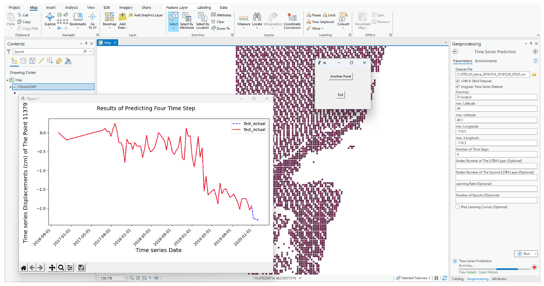
3.4. Integration of LSTM, TG-LSTM and TFT Models into ArcGIS Pro Toolbox

To enable the advanced forecasting of displacement time series within a geospatial context, we developed a toolbox that incorporates LSTM, TG-LSTM, and TFT models into the ArcGIS Pro environment. The toolbox is designed to accommodate both regularly and irregularly sampled time series. Instead of automatically detecting sampling regularity, the toolbox relies on user input. When the checkbox indicating a non-regular dataset is selected, the data is interpreted as irregular, prompting the application of the TG-LSTM model for single-step prediction and the TFT model for multi-step forecasting; otherwise, the toolbox defaults to the LSTM architecture. This mechanism supports both next-step and multi-step forecasting.

The toolbox architecture extracts displacement values and associated temporal features from input time series. For datasets identified as irregular, time intervals are incorporated as an additional input feature to enhance temporal modeling. For regularly spaced series, this step is omitted. The toolbox provides advanced configuration options, including customizable hyperparameters (e.g., number of LSTM units, learning rate, number of training epochs), and offers real-time visualization of learning curves to track convergence during training.

Full compatibility with Sentinel-1 displacement datasets is ensured via a dedicated protocol for products processed through the Italian National Council of Research (CNR) P-SBAS service on the G-TEP platform. Furthermore, the toolbox supports external datasets that have not undergone P-SBAS processing, provided they conform to the structural requirements outlined in

Table 4. Expected dataset structure for compatibility with the toolbox when using data not generated by the P-SBAS service.

ID	Lat	Lon	26 January 2018	7 February 2018	19 February 2018	3 March 2018	15 March 2018
0	38.7079	−9.4854	0	0.0004	0.1624	0.1624	0.3414
1	38.7088	−9.4863	0	0.0016	0.0385	0.0385	0.3324
2	38.7096	−9.4863	0	0.0031	0.1335	0.1335	0.2479
3	38.7096	−9.4863	0	0.0052	0.4813	0.4813	0.5352
4	38.7104	−9.4863	0	0.0071	0.3348	0.3348	0.4225
5	38.7071	−9.4846	0	0.0831	−0.0141	−0.0141	0.2588
6	38.7079	−9.4846	0	−0.0023	0.1143	0.1143	0.2320
7	38.7079	−9.4846	0	−0.1181	0.0620	0.0620	0.1224
8	38.7088	−9.4854	0	−0.2369	0.4562	0.4562	0.2081
9	38.7096	−9.4854	0	0.0018	0.2273	0.2273	0.2738

.

Users are required to define the geographical extent of the analysis explicitly. This spatial specification is essential for constraining the processing domain and is reinforced by internal safeguards that manage computational load for large-scale datasets.

The motivation behind this toolbox lies in bridging the gap between advanced deep learning models and operational geospatial workflows. By embedding forecasting capabilities directly within ArcGIS Pro, the toolbox allows geoscientists, urban planners, and hazard managers to perform time series predictive modeling without requiring separate coding environments. This spatial integration facilitates intuitive selection of areas of interest, point-specific forecasting, and overlay with other geospatial layers—thereby enhancing interpretability and decision making. The value of this approach is in its ability to transform DL-based InSAR forecasting from a research task into an applied, location-aware tool accessible within established GIS ecosystems. The detailed configuration instructions, usage guidelines, and source code for the toolbox are available in the public GitHub repository: https://github.com/Lama-NM/displacement-forecasting-toolbox-ArcGISPRO (accessed on 21 September 2021).

Given the integration of various techniques in the proposed method, a workflow diagram (see Figure 5) is presented to outline the end-to-end implementation process:

4. Results

This section presents the evaluation of forecasting models applied to displacement time series. We first examine the application of LSTM models for single- and multi-step forecasting in regular datasets. Strategies for addressing irregular time series are then assessed, comparing imputation with time-interval embedding. The performance of the TG-LSTM and TFT models is analyzed. Finally, we outline the integration of the LSTM, TG-LSTM, and TFT models into a GIS-based toolbox within the ArcGIS Pro environment.

4.1. Models Evaluation and Validation

We compare the LSTM, TG-LSTM, and TFT models for forecasting regular and irregular displacement time series. The analysis relies on three datasets generated using the P-SBAS technique. We also evaluate the impact of the preprocessing methods described earlier. An ensemble approach based on five-fold cross-validation is employed. Each model’s contribution is weighted inversely to its validation RMSE, giving more influence to models with lower errors. This ensemble model applied the weights, scaled the predictions, and averaged them, enhancing both accuracy and stability on the test set.

4.1.1. Outcomes of Time Series Forcasting for Regular Displacement Patterns

The regular dataset examined in this study is the Lombardy dataset, which spans 50 time steps.

• One Time Step Prediction
  All hyperparameters for predicting one time step are listed in

  Table 5. Comparison of hyperparameters for training an LSTM Model to predict one time step versus multiple time steps (Lombardy dataset).

  Hyperparameter	One Time Step	Multiple Time Steps
  Num. of LSTM Layers	1	2
  Num. of Nodes	50	100, 50
  Num. of Epochs	15	35
  Learning Rate	0.001	0.0001
  Optimizer	Adam	Adam
  Loss Function	custom L1-L2	custom L1-L2
  Accuracy Metric	RMSE	RMSE
  Batch Size	128	128
  Cross-Fold Validation	5 folds	5 folds

  . The model used a custom loss function that combines L1 (Mean Absolute Error) and L2 (Mean Squared Error) components. These were weighted using the parameters alpha and beta. By setting alpha to 0.3 and beta to 0.7, we placed more weight on L2 loss. This helped reduce larger errors while still being robust to outliers. Reference [67] contains detailed descriptions of the basic and advanced definitions of DL model parameters and hyperparameters.
  The displacement values in the dataset ranged from −4.1 cm to 3.2 cm, with a standard deviation of 0.4 cm. Based on this distribution, the model’s average RMSE, evaluated on a split of the dataset (80% for training and validation, 20% for testing, consistently applied across all datasets), was recorded at 0.08 cm. This relatively low RMSE, when compared to the overall range and variability of the displacement values, indicates that the model is capable of reliably approximating the underlying patterns in the data. The small difference between the predicted and observed values shows that the model captures detailed displacement trends effectively.
• Multiple Time Step Prediction
  For multi-step forecasting, we used an enhanced LSTM model based on the single-step version. This updated model demonstrated strong performance. The corresponding hyperparameters are listed in Table 5.
  To assess the model’s reliability in predicting a sequence of up to fourteen time steps within a 50-step time series, two critical diagnostic checks were performed: plotting the ACF (autocorrelation function) and evaluating homoscedasticity.

  –

  ACF: The Autocorrelation Function (ACF) measures the linear relationship between observations separated by time lags in the sequence [68]. Plotting the ACF is essential as it reveals any remaining correlation in the residuals of the model’s predictions. Significant autocorrelation at any lag suggests that the model has not fully captured the predictive structure within the data, indicating room for improvement. Conversely, the absence of such correlation would affirm that the model’s predictions are not systematically biased by overlooked temporal dependencies.

  –

  Homoscedasticity: Homoscedasticity indicates that prediction errors have a consistent variance across all input values. This is an important condition for statistical validity. Heteroscedasticity may indicate that the model is missing important features, contains misspecifications, or requires variable transformations. This condition is foundational for the validity of various statistical inferences made based on the model, as described in [69].

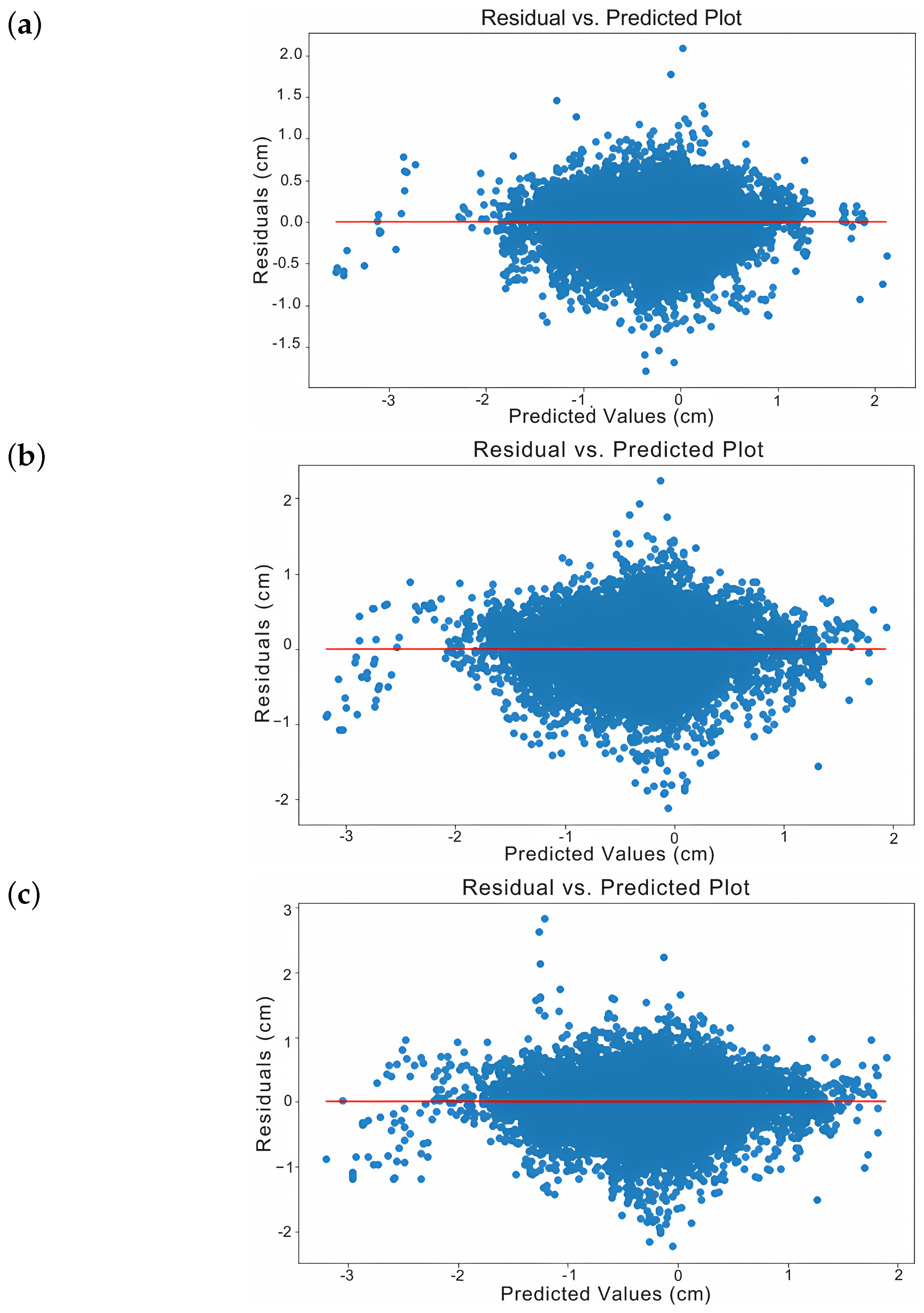
  The training results showed consistent improvement in both loss and RMSE over six, ten, and fourteen prediction steps. The validation results followed a similar trend. There was no sign of overfitting. The model balanced bias and variance well and generalized effectively to unseen data. As shown in Figure 6, Figure 6a displays a more homoscedastic error pattern than Figure 6b,c.
  This is demonstrated by the reduced number of outliers and tighter error containment around zero, indicating stable variance in prediction errors across different predicted values. The residuals are also symmetrically distributed above and below the zero line without a funnel shape, reinforcing the presence of homoscedasticity. Figure 7 shows that as the prediction range increases—from six to fourteen steps—outlier errors become more frequent. This suggests higher uncertainty in longer-term forecasts.
  Figure 8 shows the ACF for predicting fourteen time steps. It reveals that autocorrelation remains minimal and stable up to five steps but increases significantly beyond this point. This pattern suggests that autocorrelation grows as predictions extend further. This is expected in physical systems where each time step continues the same process. Such systems often show correlation between successive stages.
  Consequently, forecasts beyond five steps may compromise accuracy, while predictions within this range maintain reliability. Thus, to ensure accuracy while maintaining temporal coverage, we used 10% of the series length as a benchmark. This was applied to the Lisbon (48 steps) and Washington (75 steps) datasets. Figure 9 shows examples of six, ten, and fourteen predicted time steps for the time series number 4395 of the dataset.

4.1.2. Outcomes of Time Series Forecasting for Irregular Displacement Patterns

The explored irregular datasets are the Lisbon and Washington datasets.

• One-Time-Step Prediction

  -

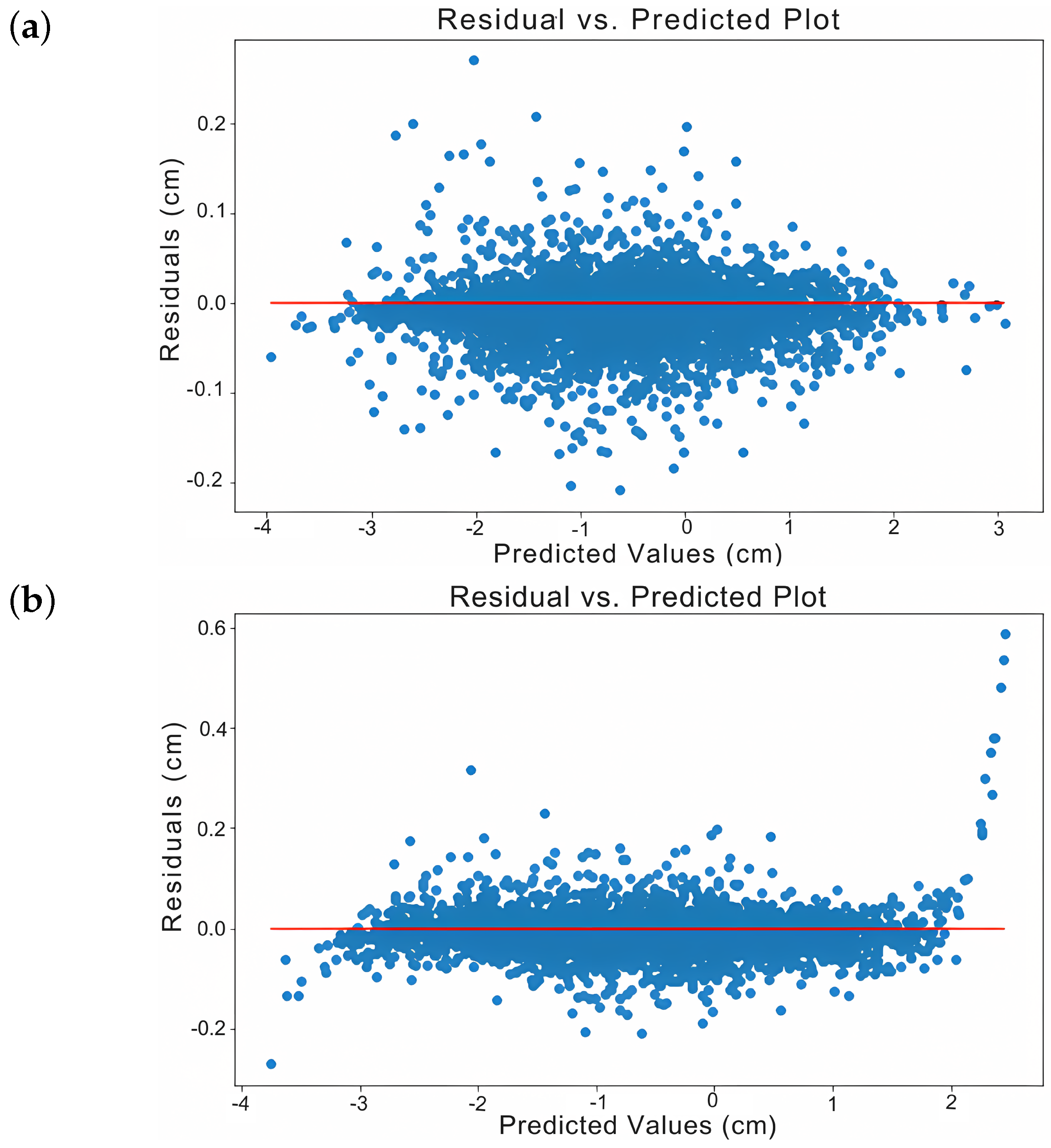
  Lisbon Dataset Results:

  We applied the LSTM model to the Lisbon dataset using the same architecture as for the Lombardy dataset. However, we increased the number of epochs from 15 to 35 and expanded the dataset to 109,962 samples, with displacement values ranging from −6.5 cm to 3.8 cm.

  We excluded the ACF analysis because it works well when time is used as a feature but not when missing values are imputed, where artificial correlations may be introduced. Therefore, it was deemed more appropriate to exclude it from this comparison.

  After training, we observed the learning curves of both models—one incorporating missing value imputation and the other embedding time intervals as a second feature. Both models learned rapidly, with loss and RMSE values converging within the first few epochs. The key difference was in the initial loss and RMSE values. The model with time intervals started with higher errors but eventually reached similar low levels. This is likely due to its dual input of displacements and time intervals, unlike the other model. The validation and training results were closely aligned, suggesting minimal overfitting and strong generalization.

  On average, the RMSE was 0.0004 cm when implementing missing data imputation. The low RMSE with imputation may result from the smoothing effect of filled-in values and the larger dataset. When embedding time intervals as a second feature, the RMSE was 0.055 cm. To draw a more detailed conclusion, Figure 10 presents a comparative analysis of the homoscedasticity associated with the aforementioned data preprocessing techniques. Figure 10a (missing value imputation) shows better homoscedasticity, making it preferable, as it indicates that model errors are evenly distributed and stable across predictions. Figure 10b (time interval embedding) shows greater residual variability, especially as predictions move away from zero. This indicates heteroscedasticity, where error magnitude depends on the predicted value. The homoscedasticity plots in this paper represent only displacement residuals.

  -

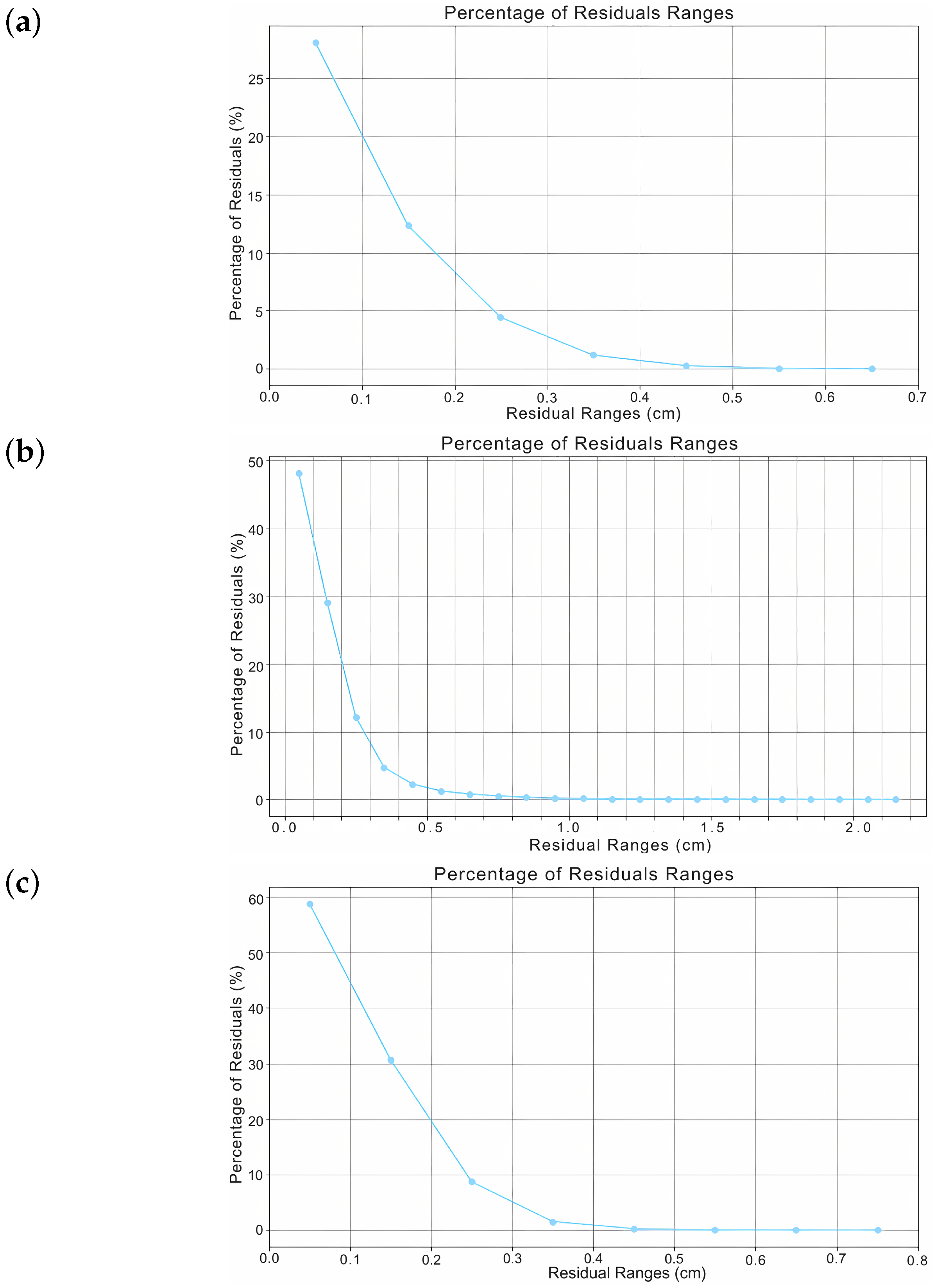
  Washington Dataset Results:

  We trained the Washington dataset using the same hyperparameters as for the Lisbon dataset. The only difference was a smaller sample size—21,471 records, ranging from −5.1 cm to 4.1 cm. Learning curves showed rapid improvement, with sharp drops in both loss and RMSE. This trend was similar to what was observed in the Lisbon single-step forecast. Initially higher errors were caused by the added complexity of using time interval embeddings. Despite this, both models generalized well. The validation metrics stayed close to the training results, reducing concerns about overfitting. The consistently lower loss and RMSE values suggested effective model performance across datasets. On average, the RMSE was 0.036 cm with missing data imputation and 0.03 cm with time interval integration.

  Figure 11 presents a comparative analysis of the homoscedasticity associated with missing data imputation and embedding time intervals as a second feature. Figure 11a (missing value imputation) exhibits better homoscedasticity, with residuals evenly distributed around zero across the predicted values. This consistency is desirable, as it indicates a uniform distribution of errors. In contrast, Figure 11b (time interval embedding) displays a "fan-shaped" spread of residuals. This indicates that errors increase with higher predicted values, suggesting variability in accuracy.

  Furthermore, the residual distribution plots in Figure 12 support the previous observations. In Figure 12a (missing value imputation), nearly all residuals fall within a narrow range, indicating consistent, low error, and better homoscedasticity. Figure 12b (embedding time intervals) shows residuals distributed over a broader range, reflecting greater variability and heteroscedasticity. All residual plots in this paper show absolute displacement errors. We excluded time interval errors due to their negligible magnitude.

  Overall, the model using missing data imputation generally performed better than the one using time interval embedding.

• Multiple-Time-Step Prediction
  Because some heteroscedasticity persisted, we tested the TG-LSTM model, which is designed to handle irregular time intervals. While TG-LSTM mitigated some of these issues, it was computationally expensive and still exhibited outliers.
  Consequently, we transitioned to the TFT model for improved performance. The LSTM model used in this task was configured with hyperparameters comparable to those applied in Lombardy’s multi-step time series forecasting. Unlike the LSTM, the TG-LSTM model incorporated time as a second feature and utilized a dual-layer architecture, as described in Section 3.2.
  The TFT model architecture in this study is specifically tailored to predict both displacement and time intervals in multi-step time series. Its architecture begins with an LSTM encoder layer (eight units), followed by a multi-head attention layer with two heads and a key size of eight. The attention output passes through a Gated Residual Network (GRN), implemented as a dense layer with eight nodes and ReLU activation. This setup includes a residual connection and layer normalization for training stability.

  -

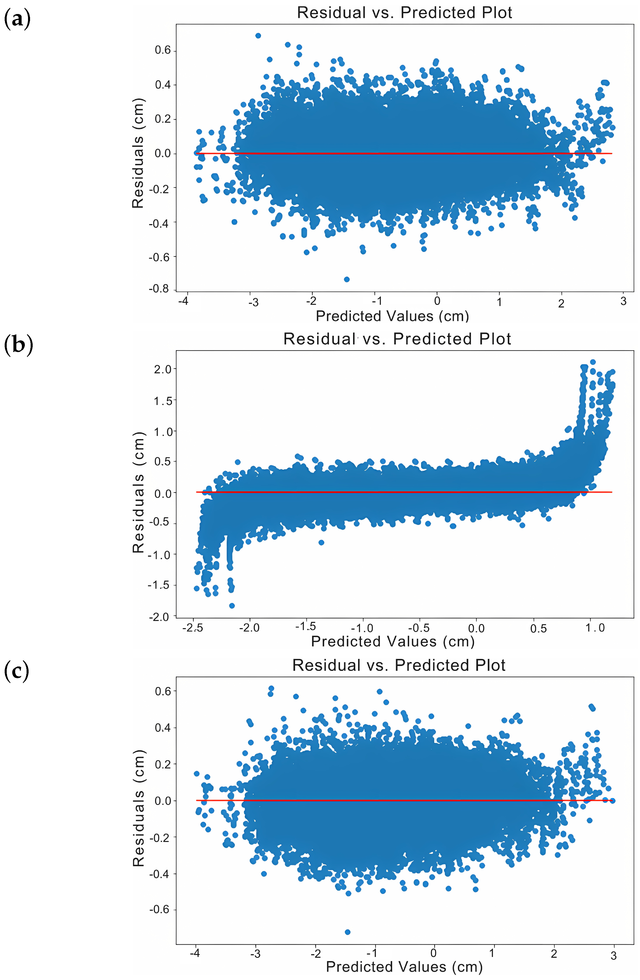
  Lisbon Dataset Results

  All three models showed good convergence, with training and validation curves aligning quickly.

  Table 6. RMSE and computation cost for the standard LSTM, TG-LSTM, and TFT models, respectively (Lisbon dataset).

  Model	RMSE (cm)	MAE (cm)	Computation Cost (min)
  Standard LSTM	0.124	0.085	287
  TG-LSTM	0.169	0.125	288
  TFT	0.167	0.128	84

  reports the RMSE, Mean Absolute Error (MAE), and computation time. The TFT model achieved both low error and the shortest run time. Since the computational time depends on the system’s processor and memory, we note that the experiments were conducted on a machine equipped with an AMD Ryzen 7 5700U processor (8 cores, 16 threads, 1801 MHz) and 16 GB of RAM.

  Figure 13 illustrates the influence of homoscedasticity on the standard LSTM, TG-LSTM, and TFT models. The standard LSTM model (Figure 13a) exhibited scattered residuals with variable spread, indicating some heteroscedasticity and leading to inconsistent error distribution across predictions. Figure 13b (TG-LSTM) showed a better residual concentration around zero compared to LSTM, but still displayed variability at extreme values and remained sensitive to outliers. In contrast, the TFT model (Figure 13c) showed the most consistent residual spread around zero, demonstrating the most favorable homoscedasticity. Its strength in capturing dependencies and handling irregular time steps made TFT the most reliable model.

  In addition to the residual-based evaluation, we also report the MAE to provide a complementary view of average prediction accuracy. For the Lisbon dataset, the LSTM model achieved the lowest MAE, followed by TG-LSTM and TFT. Although LSTM achieves better average performance, the residual plots indicate that this comes at the cost of increased variance and reduced error stability—particularly at the edges of the prediction range. In contrast, TFT’s slightly higher MAE is compensated for by its more homoscedastic and symmetric residual distribution.

  Furthermore, the residual distribution plots (Figure 14) support the earlier conclusions. Figure 14c shows the narrowest error range and the highest residual concentration, aligning with TFT’s strong stability and homoscedasticity. Figure 14b (TG-LSTM) has broader residuals than TFT but they are still slightly narrower than in the standard LSTM. The standard LSTM model (Figure 14a) presents the widest spread of residuals, confirming higher error variability. These observations further highlight that the TFT model manages residuals more effectively, providing better stability and generalization in predictions.

  Figure 15 presents an example of multi-step predictions using the three models for time series index 11,840. The difference in the number of time steps is due to missing value imputation in the dataset. Originally consisting of 48 displacement data points, the dataset expanded to 138 points after imputation. Consequently, 10% of the time series now corresponds to 5 time steps in the original dataset and 14 time steps in the imputed dataset. Another example of multi-step forecasting results for time series number 9691 is presented in Appendix B, reinforcing the comparative evaluation of the three models.

  -

  Washington Dataset Results:

  The same three models were subsequently applied to the Washington dataset, with the training epoch count adjusted to 50. They were assessed on 10% of the time series length, corresponding to eight steps. Overall, the models appeared to learn effectively without overfitting, as evidenced by the convergence and parallel behavior of the training and validation loss/RMSE curves.

  Table 7. RMSE and computation cost for the standard LSTM, TG-LSTM, and TFT models, respectively (Washington dataset).

  Model	RMSE (cm)	MAE (cm)	Computation Cost (min)
  Standard LSTM	0.127	0.099	55
  TG-LSTM	0.224	0.134	115
  TFT	0.125	0.11	85

  presents the RMSE, MAE, and computation time values for each model. The results indicate that the TFT model outperformed the TG-LSTM in both predictive accuracy and computational efficiency. Compared to standard LSTM, TFT required more computational time and achieved a slightly lower RMSE; however, the difference between the two was minimal. The MAE results followed a similar trend, with TFT and LSTM showing comparable performance and TG-LSTM exhibiting the highest average error. While LSTM achieved the lowest MAE, the difference from TFT was small, and, as shown in the residual plots, TFT maintained superior stability and consistency, which are essential in irregular, multi-step forecasting. Despite the higher computational cost, TFT remains the most robust option. Its dual input of displacement and time intervals allows for a higher-dimensional data representation. Unlike standard LSTM, which excluded the first two time steps to avoid bias from large gaps, the TFT model retained all data, better capturing time-based variation. Therefore, its higher cost is justified by improved accuracy and handling of continuous time series.

  Figure 16 illustrates the homoscedasticity for the three models. The TFT model (Figure 16c) demonstrates the best homoscedasticity, with residuals most evenly distributed around zero and no discernible pattern. The standard LSTM model (Figure 16a) follows closely, though it shows slightly denser clusters at certain predicted values, suggesting minor issues with variance consistency. Figure 16b (TG-LSTM) shows a funnel-shaped residual pattern, with growing error variance at higher prediction values, confirming heteroscedasticity.

  The residual distribution plots in Figure 17 confirm that the TFT model offers the best consistency in error distribution, followed by the standard LSTM. The TG-LSTM model shows the greatest variability, with a broader spread and residuals extending to larger ranges.

  Figure 18 shows an example of predicting multiple time steps using the three models for the time series number 1904. A second example illustrating multi-step predictions for time series number 828 is provided in Appendix B, further supporting the comparative analysis across models.

• Overall Summary
  According to the results, the learning curves from the Lisbon and Washington datasets did not provide definitive evidence to identify a single best-performing model overall. However, the Lisbon multi-step analysis showed that the TFT model performed best in terms of homoscedasticity, residual distribution, and computational cost.
  While the TFT had a slightly higher RMSE than the standard LSTM—mainly due to a few large residuals—this metric should be interpreted with caution. Residual plots show that the TFT model produced more predictions with residuals below 0.1 cm than the others. This indicates that, despite a few extreme values, the TFT model consistently delivered high-accuracy predictions for the majority of the dataset. This is important in practical applications, where consistent accuracy matters more than rare large errors.
  Comparable results were observed for the Washington dataset, further supporting the superior performance of the TFT model. Qualitative examples further show that the TFT model accurately captured subtle displacement changes over time.

4.2. The Developed Toolbox Workflow in ArcGIS Pro

Upon execution, the toolbox guides the user through defining the dataset properties, including temporal regularity and geographic extent. Based on the selection (e.g., checking the “Irregular Time Series Dataset” box), the appropriate forecasting model is triggered automatically, as previously detailed in Section 3.4.

Following initial execution, two primary outputs are generated:

• A shapefile containing the spatial coordinates (latitudes and longitudes) of the points specified by the user and referenced to the time series dataset.
• A notification displaying the RMSE obtained from training the predictive model.

Upon completion of the training phase, a Tkinter-based graphical interface is activated to facilitate the visualization of the predictive results for different points. If multiple points are selected simultaneously, an error message is triggered to enforce single-point selection.

Dynamic updating of the displayed prediction occurs whenever the user selects a different point by clicking within the interface. An example of forecasting four future time steps using the toolbox is presented in Figure 19.

The overall implementation logic, developed in Python and integrating geospatial processing, deep learning, and interactive visualization, is summarized in the workflow diagram (Figure 20).

This architecture supports the full forecasting of regular and irregular displacement series with minimal user input.

5. Conclusions

This study explored LSTM-based models for forecasting ground displacements in both regular and irregular time series. For irregular series, imputing missing values outperformed embedding time intervals when using standard LSTMs, although standard models showed limitations in multi-step prediction tasks.

To address this, we implemented TG-LSTM and TFT models, which directly incorporate time intervals into their architecture. Among these, the TFT model demonstrated superior performance, improving predictive reliability and reducing computational cost, as confirmed by homoscedasticity and RMSE analyses. Quantitatively, TFT achieved RMSE values of 1.71 mm/year for Lisbon and 1.26 mm/year for Washington, outperforming TG-LSTM and standard LSTM in multi-step forecasting. Alongside model development, we introduced a GIS-integrated forecasting toolbox that automatically selects the appropriate model based on data regularity, combining deep learning techniques with InSAR analysis in a practical geospatial framework. While LSTM proved sufficient for the regular dataset, the architectural strengths of TFT suggest it could also be advantageous for forecasting regular time series. The findings highlight the importance of tailoring model architectures to data characteristics.

Future work will focus on integrating environmental covariates, such as temperature, precipitation, and topographical features, to enhance model interpretability and accuracy. Further development of the toolbox will also aim to incorporate statistical evaluation tools and expand hyperparameter customization, offering greater flexibility and robustness for geospatial time series forecasting.

References

- Crosetto, M.; Monserrat, O.; Cuevas-González, M.; Devanthéry, N.; Crippa, B. Persistent scatterer interferometry: A review. ISPRS J. Photogramm. Remote Sens. 2016, 115, 78–89. [Google Scholar] [CrossRef]
- Macchiarulo, V.; Milillo, P.; Blenkinsopp, C.; Reale, C.; Giardina, G. Multi-temporal InSAR for transport infrastructure monitoring: Recent trends and challenges. In Proceedings of the Institution of Civil Engineers-Bridge Engineering; Thomas Telford Ltd.: London, UK, 2021; Volume 176, pp. 92–117. [Google Scholar] [CrossRef]
- Gama, F.F.; Mura, J.C.; Paradella, W.R.; de Oliveira, C.G. Deformations prior to the Brumadinho dam collapse revealed by Sentinel-1 InSAR data using SBAS and PSI techniques. Remote Sens. 2020, 12, 3664. [Google Scholar] [CrossRef]
- Romanuke, V. Arima Model Optimal Selection for Time Series Forecasting. Marit. Tech. J. 2022, 224, 28–40. [Google Scholar] [CrossRef]
- Jiang, W.; Ling, L.; Zhang, D.; Lin, R.; Zeng, L. A time series forecasting model selection framework using CNN and data augmentation for small sample data. Neural Process. Lett. 2023, 55, 5783–5810. [Google Scholar] [CrossRef]
- Zhang, G.P.; Qi, M. Neural network forecasting for seasonal and trend time series. Eur. J. Oper. Res. 2005, 160, 501–514. [Google Scholar] [CrossRef]
- Liu, Q.; Li, Z.; Ji, Y.; Martinez, L.; Zia, U.H.; Javaid, A.; Lu, W.; Wang, J. Forecasting the Seasonality and Trend of Pulmonary Tuberculosis in Jiangsu Province of China Using Advanced Statistical Time-Series Analyses. Infect. Drug Resist. 2019, 12, 2311–2322. [Google Scholar] [CrossRef]
- Song, L.; Ding, L.; Wen, T.; Yin, M.; Zeng, Z. Time series change detection using reservoir computing networks for remote sensing data. Int. J. Intell. Syst. 2022, 37, 10845–10860. [Google Scholar] [CrossRef]
- Ji, X.; Zhang, H.; Li, J.; Zhao, X.; Li, S.; Chen, R. Multivariate time series prediction of high dimensional data based on deep reinforcement learning. In Proceedings of the International Conference on Power System and Energy Internet (PoSEI2021), Chengdu, China, 16–18 April 2021; Volume 256, p. 02038. [Google Scholar] [CrossRef]
- Lai, K.H.; Zha, D.; Xu, J.; Zhao, Y.; Wang, G.; Hu, X. Revisiting Time Series Outlier Detection: Definitions and Benchmarks. In Proceedings of the Thirty-Fifth Conference on Neural Information Processing Systems Datasets and Benchmarks Track (Round 1), Online, 6–14 December 2021. [Google Scholar]
- Bauer, A. Automated Hybrid Time Series Forecasting: Design, Benchmarking, and Use Cases. Ph.D. Thesis, Universitat Würzburg, Würzburg, Germany, 2021. [Google Scholar]
- Weerakody, P.B.; Wong, K.W.; Wang, G.; Ela, W. A review of irregular time series data handling with gated recurrent neural networks. Neurocomputing 2021, 441, 161–178. [Google Scholar] [CrossRef]
- Rehfeld, K.; Marwan, N.; Heitzig, J.; Kurths, J. Comparison of correlation analysis techniques for irregularly sampled time series. Nonlinear Process. Geophys. 2011, 18, 389–404. [Google Scholar] [CrossRef]
- Zhang, K.; Ng, C.T.; Na, M.H. Real time prediction of irregular periodic time series data. J. Forecast. 2020, 39, 501–511. [Google Scholar] [CrossRef]
- Tan, Q.; Ye, M.; Yang, B.; Liu, S.; Ma, A.J.; Yip, T.C.F.; Wong, G.L.H.; Yuen, P. Data-gru: Dual-attention time-aware gated recurrent unit for irregular multivariate time series. In Proceedings of the AAAI Conference on Artificial Intelligence, New York, NY, USA, 7–12 February 2020; Volume 34, pp. 930–937. [Google Scholar] [CrossRef]
- Kidger, P.; Morrill, J.; Foster, J.; Lyons, T. Neural controlled differential equations for irregular time series. Adv. Neural Inf. Process. Syst. 2020, 33, 6696–6707. [Google Scholar] [CrossRef]
- Siami-Namini, S.; Tavakoli, N.; Namin, A.S. A comparison of ARIMA and LSTM in forecasting time series. In Proceedings of the 17th IEEE International Conference on Machine Learning and Applications (ICMLA), Orlando, FL, USA, 17–20 December 2018; pp. 1394–1401. [Google Scholar]
- Colak, I.; Sagiroglu, S.; Yesilbudak, M.; Kabalci, E.; Bulbul, H.I. Multi-time series and -time scale modeling for wind speed and wind power forecasting part I: Statistical methods, very short-term and short-term applications. In Proceedings of the International Conference on Renewable Energy Research and Applications (ICRERA), Palermo, Italy, 22–25 November 2015; pp. 209–214. [Google Scholar] [CrossRef]
- Dilling, S.; MacVicar, B. Cleaning high-frequency velocity profile data with autoregressive moving average (ARMA) models. Flow Meas. Instrum. 2017, 54, 68–81. [Google Scholar] [CrossRef]
- Dubey, A.K.; Kumar, A.; García-Díaz, V.; Sharma, A.K.; Kanhaiya, K. Study and analysis of SARIMA and LSTM in forecasting time series data. Sustain. Energy Technol. Assess. 2021, 47, 101474. [Google Scholar] [CrossRef]
- Alharbi, F.R.; Csala, D. A seasonal autoregressive integrated moving average with exogenous factors (SARIMAX) forecasting model-based time series approach. Inventions 2022, 7, 94. [Google Scholar] [CrossRef]
- Connolly, E. The Suitability of Sarimax Time Series and LSTM Neural Networks for Predicting Electricity Consumption in Ireland. Ph.D. Thesis, National College of Ireland, Dublin, Ireland, 2021. [Google Scholar]
- Gelper, S.; Fried, R.; Croux, C. Robust forecasting with exponential and Holt–Winters smoothing. J. Forecast. 2010, 29, 285–300. [Google Scholar] [CrossRef]
- Hill, P.; Biggs, J.; Ponce-López, V.; Bull, D. Time-Series Prediction Approaches to Forecasting Deformation in Sentinel-1 InSAR Data. J. Geophys. Res. Solid Earth 2021, 126, e2020JB020176. [Google Scholar] [CrossRef]
- Fiorentini, N.; Maboudi, M.; Leandri, P.; Losa, M. Can Machine Learning and PS-InSAR Reliably Stand in for Road Profilometric Surveys? Sensors 2021, 21, 3377. [Google Scholar] [CrossRef]
- Radman, A.; Akhoondzadeh, M.; Hosseiny, B. Integrating InSAR and Deep-Learning for Modeling and Predicting Subsidence over the Adjacent Area of Lake Urmia, Iran. GISci. Remote Sens. 2021, 58, 1413–1433. [Google Scholar] [CrossRef]
- Abdikan, S.; Coskun, S.; Narin, O.G.; Bayik, C.; Calò, F.; Pepe, A.; Balik Sanli, F. Prediction of Long-Term SENTINEL-1 InSAR Time Series Analysis. Int. Arch. Photogramm. Remote Sens. Spat. Inf. Sci. 2023, 48, 3–8. [Google Scholar] [CrossRef]
- Mirmazloumi, S.M.; Wassie, Y.; Nava, L.; Cuevas-González, M.; Crosetto, M.; Monserrat, O. InSAR Time Series and LSTM Model to Support Early Warning Detection Tools of Ground Instabilities: Mining Site Case Studies. Bull. Eng. Geol. Environ. 2023, 82, 374. [Google Scholar] [CrossRef]
- Lattari, F.; Rucci, A.; Matteucci, M. A Deep Learning Approach for Change Points Detection in InSAR Time Series. IEEE Trans. Geosci. Remote Sens. 2022, 60, 5223916. [Google Scholar] [CrossRef]
- Wang, J.; Li, C.; Li, L.; Huang, Z.; Wang, C.; Zhang, H.; Zhang, Z. InSAR Time-Series Deformation Forecasting Surrounding Salt Lake Using Deep Transformer Models. Sci. Total Environ. 2023, 858, 159744. [Google Scholar] [CrossRef] [PubMed]
- Wang, J.; Fan, X.; Zhang, Z.; Zhang, X.; Nie, W.; Qi, Y.; Zhang, N. Spatiotemporal Mechanism-Based Spacetimeformer Network for InSAR Deformation Prediction and Identification of Retrogressive Thaw Slumps in the Chumar River Basin. Remote Sens. 2024, 16, 1891. [Google Scholar] [CrossRef]
- Gualandi, A.; Liu, Z. Variational Bayesian Independent Component Analysis for InSAR Displacement Time-Series with Application to Central California, USA. J. Geophys. Res. Solid Earth 2021, 126, e2020JB020845. [Google Scholar] [CrossRef]
- Geohazards-TEP. Geohazard Exploitation Platform. Available online: https://geohazards-tep.eu/#! (accessed on 21 September 2021).
- Manunta, M.; De Luca, C.; Zinno, I.; Casu, F.; Manzo, M.; Bonano, M.; Fusco, A.; Pepe, A.; Onorato, G.; Berardino, P.; et al. The Parallel SBAS Approach for Sentinel-1 Interferometric Wide Swath Deformation Time-Series Generation: Algorithm Description and Products Quality Assessment. IEEE Trans. Geosci. Remote Sens. 2019, 57, 6259–6281. [Google Scholar] [CrossRef]
- Cuervas-Mons, J.; Zêzere, J.L.; Domínguez-Cuesta, M.J.; Barra, A.; Reyes-Carmona, C.; Monserrat, O.; Oliveira, S.C.; Melo, R. Assessment of Urban Subsidence in the Lisbon Metropolitan Area (Central-West of Portugal) Applying Sentinel-1 SAR Dataset and Active Deformation Areas Procedure. Remote Sens. 2022, 14, 4084. [Google Scholar] [CrossRef]
- Seabold, S.; Perktold, J. Statsmodels: Econometric and statistical modeling with python. In Proceedings of the 9th Python in Science Conference, Austin, TX, USA, 28 June–3 July 2010; Volume 57, p. 61. [Google Scholar] [CrossRef]
- Harvey, A.C. Forecasting, Structural Time Series Models and the Kalman Filter; Cambridge University Press: Cambridge, UK, 1990. [Google Scholar] [CrossRef]
- Pelagatti, M.M. Time Series Modelling with Unobserved Components; CRC Press: Boca Raton, FL, USA, 2015. [Google Scholar]
- Costa, P.; Cerqueira, V.; Vinagre, J. AutoFITS: Automatic Feature Engineering for Irregular Time Series. arXiv 2021, arXiv:2112.14806. [Google Scholar] [CrossRef]
- Viganò, A.; Rossato, S.; Martin, S.; Ivy-Ochs, S.; Zampieri, D.; Rigo, M.; Monegato, G. Large Landslides in the Alpine Valleys of the Giudicarie and Schio-Vicenza Tectonic Domains (NE Italy). J. Maps 2021, 17, 197–208. [Google Scholar] [CrossRef]
- Guzzetti, F. Landslide fatalities and the evaluation of landslide risk in Italy. Eng. Geol. 2000, 58, 89–107. [Google Scholar] [CrossRef]
- ISPRA. Rapporto Dissesto Idrogeologico Italia Ispra 356_2021; ISPRA: Rome, Italy, 2021; p. 183. [Google Scholar]
- Pereira, S.; Santos, P.P.; Zêzere, J.L.; Tavares, A.O.; Garcia, R.A.C.; Oliveira, S.C. A Landslide Risk Index for Municipal Land Use Planning in Portugal. Sci. Total Environ. 2020, 735, 139463. [Google Scholar] [CrossRef]
- Terrinha, P.; Duarte, H.; Brito, P.; Noiva, J.; Ribeiro, C.; Omira, R.; Baptista, M.A.; Miranda, M.; Magalhães, V.; Roque, C.; et al. The Tagus River Delta Landslide, off Lisbon, Portugal. Implications for Marine Geo-Hazards. Mar. Geol. 2019, 416, 105983. [Google Scholar] [CrossRef]
- Xu, Y.; Schulz, W.H.; Lu, Z.; Kim, J.; Baxstrom, K. Geologic Controls of Slow-Moving Landslides Near the US West Coast. Landslides 2021, 18, 3353–3365. [Google Scholar] [CrossRef]
- Moualla, L.; Rucci, A.; Naletto, G.; Anantrasirichai, N. Learning Ground Displacement Signals Directly from InSAR-Wrapped Interferograms. Sensors 2024, 24, 2637. [Google Scholar] [CrossRef] [PubMed]
- Hochreiter, S.; Schmidhuber, J. Long Short-Term Memory. Neural Comput. 1997, 9, 1735–1780. [Google Scholar] [CrossRef]
- Zhang, Q.; Wang, H.; Dong, J.; Zhong, G.; Sun, X. Prediction of Sea Surface Temperature Using Long Short-Term Memory. IEEE Geosci. Remote Sens. Lett. 2017, 14, 1745–1749. [Google Scholar] [CrossRef]
- Wang, J.; Jin, L.; Li, X.; He, S.; Huang, M.; Wang, H. A Hybrid Air Quality Index Prediction Model Based on CNN and Attention Gate Unit. IEEE Access 2022, 10, 113343–113354. [Google Scholar] [CrossRef]
- Greff, K.; Srivastava, R.K.; Koutník, J.; Steunebrink, B.R.; Schmidhuber, J. LSTM: A Search Space Odyssey. IEEE Trans. Neural Netw. Learn. Syst. 2016, 28, 2222–2232. [Google Scholar] [CrossRef]
- Wu, Z.; King, S. Investigating Gated Recurrent Neural Networks for Speech Synthesis. In Proceedings of the IEEE International Conference on Acoustics, Speech and Signal Processing (ICASSP), Shanghai, China, 20–25 March 2016; pp. 5140–5144. [Google Scholar] [CrossRef]
- Fanta, H.; Shao, Z.; Ma, L. Forget the Forget Gate: Estimating Anomalies in Videos Using Self-contained Long Short-Term Memory Networks. In Proceedings of the Advances in Computer Graphics: 37th Computer Graphics International Conference, CGI 2020, Geneva, Switzerland, 20–23 October 2020; Springer: Cham, Switzerland, 2020; pp. 169–181. [Google Scholar] [CrossRef]
- Can, T.; Krishnamurthy, K.; Schwab, D.J. Gating Creates Slow Modes and Controls Phase-Space Complexity in GRUs and LSTMs. In Proceedings of the First Mathematical and Scientific Machine Learning Conference, Princeton, NJ, USA, 20–24 July 2020; pp. 476–511. [Google Scholar]
- Yao, L.; Guan, Y. An improved LSTM structure for natural language processing. In Proceedings of the IEEE International Conference of Safety Produce Informatization (IICSPI), Chongqing, China, 10–12 December 2018; pp. 565–569. [Google Scholar] [CrossRef]
- Wang, J.; Xue, M.; Culhane, R.; Diao, E.; Ding, J.; Tarokh, V. Speech Emotion Recognition with Dual-Sequence LSTM Architecture. In Proceedings of the ICASSP 2020—2020 IEEE International Conference on Acoustics, Speech and Signal Processing (ICASSP), Barcelona, Spain, 4–8 May 2020; pp. 6474–6478. [Google Scholar] [CrossRef]
- Sulistyo, S.; Danang, A.W.; Aji Prasetya, P.; Didik, D.A.; Almu’iini, F. LSTM-Based Machine Translation for Madurese-Indonesian. J. Appl. Data Sci. 2023, 4, 189–199. [Google Scholar] [CrossRef]
- Salman, A.G.; Heryadi, Y.; Abdurahman, E.; Suparta, W. Single Layer & Multi-layer Long Short-Term Memory (LSTM) Model with Intermediate Variables for Weather Forecasting. Procedia Comput. Sci. 2018, 135, 89–98. [Google Scholar] [CrossRef]
- Werbos, P.J. Backpropagation through time: What it does and how to do it. Proc. IEEE 1990, 78, 1550–1560. [Google Scholar] [CrossRef]
- Sahin, S.O.; Kozat, S.S. Nonuniformly Sampled Data Processing Using LSTM Networks. IEEE Trans. Neural Netw. Learn. Syst. 2018, 30, 1452–1461. [Google Scholar] [CrossRef] [PubMed]
- Lim, B.; Arık, S.; Loeff, N.; Pfister, T. Temporal Fusion Transformers for Interpretable Multi-Horizon Time Series Forecasting. Int. J. Forecast. 2021, 37, 1748–1764. [Google Scholar] [CrossRef]
- Koya, S.R.; Roy, T. Temporal Fusion Transformers for Streamflow Prediction: Value of Combining Attention with Recurrence. J. Hydrol. 2024, 637, 131301. [Google Scholar] [CrossRef]
- López Santos, M.; García-Santiago, X.; Echevarría Camarero, F.; Blázquez Gil, G.; Carrasco Ortega, P. Application of Temporal Fusion Transformer for Day-Ahead PV Power Forecasting. Energies 2022, 15, 5232. [Google Scholar] [CrossRef]
- Liao, X.; Wong, M.S.; Zhu, R.; Zhe, W. A Temporal Fusion Transformer augmented GeoAI framework for estimating hourly land surface solar irradiation. Energy AI 2025, 21, 100529. [Google Scholar] [CrossRef]
- Li, X.; Xu, Y.; Law, R.; Wang, S. Enhancing Tourism Demand Forecasting with a Transformer-Based Framework. Ann. Tour. Res. 2024, 107, 103791. [Google Scholar] [CrossRef]
- Wu, B.; Wang, L.; Zeng, Y.R. Interpretable Wind Speed Prediction with Multivariate Time Series and Temporal Fusion Transformers. Energy 2022, 252, 123990. [Google Scholar] [CrossRef]
- Laborda, J.; Ruano, S.; Zamanillo, I. Multi-Country and Multi-Horizon GDP Forecasting Using Temporal Fusion Transformers. Mathematics 2023, 11, 2625. [Google Scholar] [CrossRef]
- Goodfellow, I.; Bengio, Y.; Courville, A. Deep Learning; MIT Press: Cambridge, MA, USA, 2016. [Google Scholar]
- Atique, A.; Sharif, N.; Subrina, R.; Vishwajit, S.; Vinitha, B.; Macfie, S.J. Forecasting of total daily solar energy generation using ARIMA: A Case Study. In Proceedings of the 2019 IEEE 9th Annual Computing and Communication Workshop and Conference (CCWC), Las Vegas, NV, USA, 8–10 January 2019; pp. 114–119. [Google Scholar]
- Corbin, N.; Oliveira, R.; Raynaud, Q.; Di Domenicantonio, G.; Draganski, B.; Kherif, F.; Callaghan, M.F.; Lutti, A. Statistical analyses of motion-corrupted MRI relaxometry data. bioRxiv 2023. [Google Scholar] [CrossRef]