Abstract
As a crucial ecological barrier in China, the Greater Khingan Mountains play a vital role in global ecological security. Investigating the spatiotemporal variations in fractional vegetation cover (FVC) and the driving mechanisms behind its spatial differentiation is essential. This study introduced a KNDVI-XGeoML framework integrating the Kernel NDVI and explainable geospatial machine learning to analyze the FVC dynamics and the mechanisms driving their spatial differentiation in China’s Greater Khingan Mountains, based on which targeted ecological management strategies were proposed. The key findings reveal that (1) from 2001 to 2022, FVC showed an increasing trend, confirming the effectiveness of ecological restoration. (2) The XGeoML model successfully revealed nonlinear relationships and threshold effects between driving factors and FVC. In addition, both single-factor importance and inter-factor interaction analyses consistently showed that landform factors dominated the spatial distribution of FVC. (3) Regional heterogeneity emerged—human activities drove the northern alpine zones, while landform factors governed other areas. (4) The natural-environment-dominated zones and human-activity-dominated zones were established, and management strategies were proposed: restricting tourism in low-altitude zones, optimizing the cold-resistant vegetation at high elevations, and improving the southern soil conditions to support ecological barrier construction. The innovation lies in merging nonlinear vegetation indices with interpretable machine learning, overcoming the traditional limitations in terms of saturation effects and analyses of spatial heterogeneity. This approach enhances our understanding of high-latitude vegetation dynamics, offering a methodological advancement for precision ecological management. The spatial zoning strategy based on dominant drivers provides actionable insights for maintaining this critical ecological barrier, particularly under climate change pressures. The framework demonstrates strong potential for extrapolation to other ecologically sensitive regions requiring data-driven conservation planning.
1. Introduction
Global climate changes and increasing human activities have posed unprecedented challenges to terrestrial ecosystems [1]. As a crucial link connecting the soil, atmosphere, and water [2], vegetation plays a vital role in maintaining ecosystem balance by regulating the energy flow and material exchange among these components [3]. The dynamics of vegetation not only reflect ecosystem stability but also provide critical insights into the response of regional ecosystems to global climate change and human activities. Therefore, investigating the spatial and temporal patterns of vegetation changes and their driving factors is essential for improving humans’ adaptive capacity in response to climate change. However, accurately quantifying vegetation changes and elucidating their driving mechanisms remain a major scientific challenge in terrestrial ecosystem research [4].
As a core indicator for quantifying vegetation community growth on the Earth’s surface, fractional vegetation cover (FVC) plays a crucial role in dynamically monitoring vegetation growth, evaluating ecosystem health, and analyzing long-term environmental trends [5]. FVC is typically defined as the percentage of the vertical projection area of vegetation (including leaves, stems, and branches) on the ground relative to the total area of the statistical region. It serves as a crucial parameter for characterizing surface vegetation coverage. Studying FVC dynamics not only reflects vegetation growth status but also helps uncover complex interactions among vegetation, the natural environment (i.e., climate, soil, and topography), and human activities [6]. The measurement of FVC primarily relies on ground measurements and remote sensing estimation [7]. Ground measurement methods are intuitive and easy to implement, having played a crucial role in early FVC monitoring [8]. However, with deepening of the research and the increasing demand for ecological monitoring, ground measurements can no longer meet the needs of modern FVC monitoring [9,10]. In contrast, remote sensing technology, which utilizes spaceborne multispectral sensors, overcomes the limitations of ground measurements and provides a powerful means for achieving large-scale and long-term FVC monitoring [11]. Inversion in remote sensing of FVC often uses methods such as empirical models, vegetation indices, and dimidiate pixel models [12]. Among these, the dimidiate pixel model has gained significant attention due to its computational efficiency, broad applicability, and high inversion accuracy. Traditional vegetation indices, such as the Normalized Difference Vegetation Index (NDVI) and the Enhanced Vegetation Index (EVI), are commonly used for FVC inversion within this model [13,14]. These indices are widely applied in assessing vegetation health and monitoring its spatial distributions. However, when analyzing regions with dense vegetation or high biomass, the NDVI and the EVI often suffer from saturation effects, leading to reduced accuracy in FVC estimation [15,16,17]. To overcome this limitation, Camps-Valls et al. proposed the Kernel Normalized Difference Vegetation Index (KNDVI), which integrates kernel-based machine learning techniques to enhance its vegetation monitoring capabilities [18]. Compared to traditional vegetation indices, the KNDVI more effectively utilizes spectral information; exhibits greater stability and robustness; and mitigates saturation effects and mixed-pixel issues [19]. As a result, integrating the KNDVI with a dimidiate pixel model offers a more accurate representation of FVC’s spatiotemporal dynamics. At present, the research on FVC inversion using the KNDVI within the dimidiate pixel model remains limited, and its full potential in FVC estimation still requires further exploration.
With the aim of obtaining high-precision FVC data, accurately analyzing the complex mechanisms of its multidimensional driving factors remains a major challenge. The traditional approaches, such as multiple linear regression, partial least squares regression, and correlation analysis [20,21,22], are limited by linear assumptions and static parameterization, making them ineffective in capturing the complex nonlinear relationships between changes in FVC and its driving factors. While machine learning models offer robustness to noise and outliers in the data [23] and can effectively identify complex interactions and nonlinear features among driving factors [24], they struggle with modeling complex spatial correlations [25]. Additionally, most machine learning models provide only global insights and fail to effectively capture the clustering effects and spatial autocorrelation of geospatial variables [26]. Although geographically weighted regression (GWR) models can account for spatial heterogeneity, their reliance on linear assumptions limits their ability to handle complex nonlinear relationships between variables [27]. This technical disconnection in the dual chain of “data inversion driving mechanism analysis” severely restricts the accurate identification of FVC’s driving factors, thereby affecting a precise assessment of the ecosystem dynamics and the scientific validity of management decisions. Therefore, there is an urgent need for a method that can simultaneously consider both the spatial relationships between FVC and its drivers and their nonlinear interactions. Such an approach would enable a comprehensive analysis and quantification of these driving factors, providing a scientific foundation for regional ecological management and sustainable development.
The XGeoML framework integrates geographically weighted (GW) models, machine learning (ML) techniques, and explainable AI (XAI) to accurately identify the driving mechanisms of FVC. It introduces the spatial weight matrix from GWR into the training process of the machine learning model using an embedded coupling strategy. This approach effectively addresses spatial heterogeneity and spatial autocorrelation among variables. It also accounts for nonlinear effects, enabling the model to capture both spatial heterogeneity and nonlinear relationships [28]. As a result, XGeoML provides a more fine-grained perspective for understanding the mechanisms driving FVC changes. The traditional machine learning algorithms are often seen as “black boxes” due to their complex internal mechanisms. This lack of transparency makes feature selection and variable weighting difficult to interpret. As a result, the models tend to have lower interpretability and reduced trust in their outcomes [29]. XGeoML integrates XAI to improve the interpretability of machine models, breaking the “black-box” effect of traditional machine learning models. However, few studies have utilized the XGeoML approach to investigate the nonlinear and spatially heterogeneous effects of drivers on FVC. This research gap urgently needs to be addressed to comprehensively explore the intricate mechanisms underlying FVC changes. A systematic evaluation of the applicability of the XGeoML model in this context is essential, as it will provide a robust theoretical foundation for the scientific management and restoration of ecosystems.
As a crucial component of China’s “two barriers and three belts” ecological security strategy [30], the Greater Khingan Mountains serve as a critical forest resource base, a climate-sensitive region, and a key carbon sink [31]. However, prolonged high-intensity forest exploitation and inadequate management have led to the degradation of most of the natural forests into structurally imbalanced, low-quality secondary forests [32]. This has weakened regional ecosystems, reducing ecological integrity and stability and the effectiveness of the ecological barrier’s function [31]. In this context, there is an urgent need to investigate the spatiotemporal dynamics of FVC and their driving mechanisms in the Greater Khingan Mountains. This will help reveal the intrinsic laws governing regional ecosystem changes. It is also essential to assess the roles and degrees of influence of various driving factors. Such insights are critical for formulating precise ecological restoration and management strategies. These efforts will provide a solid scientific basis for protecting the ecosystems of the Greater Khingan Mountains and ensuring their sustainable development. Ultimately, this research will support the reinforcement of the region’s ecological security framework. This study focuses on the Greater Khingan Mountains by constructing the KNDVI-XGeoML coupling framework and integrating TS and MK tests to analyze the spatiotemporal evolution of FVC. It further examines the nonlinear influences of key driving factors—including climate, human activities, and landform conditions—on FVC changes and their spatial heterogeneity. The objectives of this study are to (1) reveal the spatiotemporal evolution characteristics of FVC in China’s Greater Khingan Mountains; (2) validate the applicability of the XGeoML model in China’s Greater Khingan Mountains; (3) quantify the nonlinear response thresholds for key drivers and their spatial heterogeneity patterns; (4) analyze the global and local impacts of driving factors on FVC through a local interpretative model, examining both the individual effects of single factors and the interactive effects between factors; and (5) provide regionally differentiated management recommendations for the ecological protection of the Greater Khingan Mountains. These findings provide new technical ideas for identifying the driving factors behind FVC; enhance our understanding of complex regional ecosystem dynamics; and offer a scientific basis for ecological protection, carbon sink management, and sustainable development in the Greater Khingan Mountains.
2. Materials and Methods
2.1. The Study Area
The study area is located in the Greater Khingan Mountains of China, spanning 121°12′–127°00′E and 50°10′–54°33′N (Figure 1). It experiences a typical temperate monsoon climate, characterized by dry and windy springs; short, hot, and humid summers; rapidly cooling autumns with early frosts; and long, cold winters. The mean annual temperature is −5.4 °C, with the annual precipitation ranging from 200 to 500 mm. The region’s average elevation is 1200–1300 m, with slopes ranging from 5° to 20° [33].
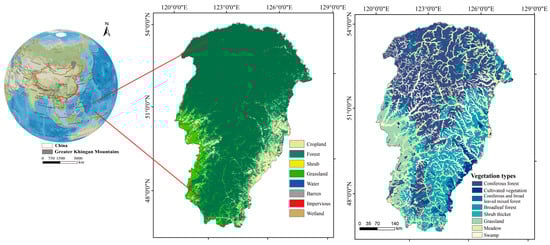
Figure 1.
The location of the study area.
2.2. The Data Collection and Processing
In this study, the vegetation index KNDVI was calculated using the MOD09GA product from MODIS based on the Google Earth Engine (GEE) platform. GEE is a cloud geospatial analysis platform developed by Google, which is specially used to process satellite images and other Earth observation data. The platform integrates massive satellite images and geospatial data resources and supports planetary-scale storage and distributed computing. MOD09GA provides daily surface reflectance data with a high temporal resolution and accurate radiometric calibration, making it well-suited to time series monitoring and vegetation index calculation at the regional scale. Leveraging the powerful distributed computing capabilities of the GEE platform, the MOD09GA data were preprocessed, and the KNDVI was extracted to ensure the stability and efficiency of large-scale remote sensing data processing.
For the selection of the driving factors, an indicator system was constructed based on three dimensions—human factors, climate factors, and landform factors—referring to relevant research findings. This system aims to quantitatively assess the influence of different types of driving forces on the spatial heterogeneity of FVC in the study area. Specifically, the human factors include GDP data, population data, and NPP-VIIRS-like nighttime light (NTL) data. Among these, the GDP and population data are non-continuous, while the NPP-VIIRS-like NTL data is continuous. To improve this research’s accuracy, multi-year raster datasets of these indicators were averaged using the Raster Calculator in ArcGIS 10.8, thereby reducing the noise caused by temporal fluctuations. Landform factors include elevation, slope, aspect, and soil type. Among these, slope and aspect were derived from the elevation data using ArcGIS’s spatial analysis tools. All of the landform datasets were based on single-year data. Climate factors were obtained from the Climatic Research Unit (CRU) dataset provided by the UK’s National Centre for Atmospheric Science (NCAS), consisting of monthly continuous meteorological records. To standardize the temporal scale and reduce the influence of seasonal variation, multi-year average raster datasets were generated using the Raster Calculator in ArcGIS 10.8.
To enhance the analytical efficiency and ensure spatial comparability across variables, all raster data were resampled to a 1 km resolution using ArcGIS 10.8 and projected using the WGS_1984_Albers coordinate system. Detailed data sources and descriptions are provided in Table 1.

Table 1.
Data information.
2.3. Methods
In this study, we first calculated the KNDVI using MOD09GA data and estimated the FVC using the dimidiate pixel model. Next, we analyzed the spatial and temporal trends in FVC using the TS median slope analysis and the MK test. Finally, we applied the XGeoML model to investigating the driving mechanisms behind FVC’s spatial differentiation. Based on these findings, we proposed targeted ecological management policies. The methodological workflow is illustrated in Figure 2.
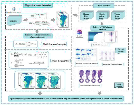
Figure 2.
A flowchart of this study.
2.3.1. Vegetation Cover Inversion
- (1)
- KNDVI calculations
The MOD09GA dataset was used to calculate the KNDVI. The MOD09GA dataset is derived from the Moderate Resolution Imaging Spectroradiometer (MODIS), which is mounted onto the Terra and Aqua satellites [34]. It is widely used to monitor surface reflectance, particularly in vegetation dynamics and ecosystem research, providing essential data for remote sensing studies and environmental monitoring. The formula for calculating the KNDVI is as follows:
where NIR represents the near-infrared band, red represents the red band, and σ denotes the length-scale parameter, which regulates the sensitivity between dense and sparse vegetation pixels or regions. In this study, we introduced an independent method to estimate σ for each pixel. This method calculates the median distance between the near-infrared and red reflectance values for each pixel, allowing the KNDVI to respond more precisely to individual pixel characteristics and adapt to their specific features better.
- (2)
- The dimidiate pixel model
FVC estimation was based on the KNDVI dataset. The formula is as follows [35].
where KNDVImax represents the KNDVI value corresponding to pure vegetation pixels, where the value at the 95th percentile of the KNDVI is adopted. KNDVImin represents the KNDVI value associated with pixels with no vegetation cover at all, where the value at the 5th percentile of the KNDVI is utilized.
2.3.2. The Spatiotemporal Variation in the FVC and a Future Trend Analysis
The Sen slope estimator is a robust non-parametric statistical method for trend analysis. It features high computational efficiency and is well-suited to analyzing long-term time series data. In this study, we employed this method to analyze the trends in the FVC. Its calculation formula is as follows:
where Median() represents the median value. If β is greater than zero, this indicates an increasing trend in FVC; otherwise, it indicates a decreasing trend.
Meanwhile, this study employed the Mann–Kendall non-parametric test to assess the significance of the trends in the vegetation index. This method is robust to the influence of certain outliers, ensuring more reliable results. The calculation formula is as follows:
where S represents the test statistic, and sgn() denotes the sign function.
Additionally, this study employs a two-sided trend test at a given significance level (set to 0.05 in this study). The specific calculation formula is provided in Equation (6), and the criteria for determining trend significance are shown in Table 2.
where Z represents the test statistic, n denotes the number of data points in the time series.
Table 2.
A significance judgment table for the trend test.
2.3.3. Identification and Analysis of the Driving Factors for FVC
- (1)
- Traditional models
In this study, to systematically assess the advantages of the XGeoML model in identifying the drivers of spatial variation in FVC in the Greater Khingan Mountains, five mainstream models were selected for a comparative analysis. These included the classical linear regression model (OLS) [36], the geographically weighted regression (GWR) model [37], multiscale geographically weighted regression (MGWR) [38], and three machine learning models—LightGBM, Gradient Boosting Regressor (GBR), and Random Forest (RF) [39,40]. Each model underwent a rigorous parameter optimization process, with the optimal parameter combinations detailed in Table 3. The input features were based on multi-year average raster data derived using the ArcGIS Raster Calculator, encompassing three dimensions: human factors, climate factors, and landform factors. The target variable was the multi-year average FVC. After the model training, the output is the FVC prediction results. The models’ accuracy was primarily evaluated using four key metrics: the coefficient of determination (R2), the root mean square error (RMSE), the mean absolute error (MAE), and the mean square error (MSE) [41]. These metrics comprehensively reflect each model’s performance in terms of the prediction accuracy, goodness of fit, and error control.
Table 3.
Model parameter optimization.
- The OLS model was implemented using the dplyr package in R 4.4.2 for data preprocessing and model construction.
- The GWR model was constructed using the GWmodel package in R 4.4.2. In this study, a bisquare kernel function was used to measure the weight relationships between samples at different spatial locations. This kernel function is characterized by a gradual decrease in weight following a bisquare function as the distance between a sample and the central point increases, effectively adjusting the weights based on sample proximity. Additionally, an adaptive bandwidth approach was employed during model construction, with the optimal bandwidth determined through cross-validation [37]. Through this optimization process, the GWR model is ensured to provide a more precise analysis of the spatial relationships in complex spatial data environments.
- The MGWR model was downloaded from the School of Geographical Sciences and Urban Planning, using a second-order kernel function to determine the bandwidth, and cross-validation was applied for verification.
- We constructed the LightGBM and Random Forest (RF) models using R 4.4.2. The RF model was implemented via the RandomForest package, with the hyperparameters mtry (number of features randomly selected at each split) and ntree (number of decision trees) optimized using the caret package. The LightGBM model was developed within the tidyverse integration framework, focusing on tuning key hyperparameters: max_depth (maximum tree depth), learning_rate, and num_leaves (number of leaf nodes). To enhance the models’ robustness and generalization, we applied stratified random sampling to splitting the dataset into training and validation sets at a 7:3 ratio. Hyperparameter optimization was performed using Grid Search (GSS), and the models’ generalization was improved further through 5-fold cross-validation.
- We constructed the GBR model using Python 3.13.2’s scikit-learn library. The model was implemented via the ensemble module, with the hyperparameters learning_rate and max_depth (maximum depth of the individual regression estimators) optimized. The model was developed within a pipeline that included preprocessing steps: one-hot encoding for categorical features (including soil) and standard scaling for numerical features. To enhance the model’s robustness and generalization, we applied random sampling to splitting the dataset into training and validation sets at a 7:3 ratio. Hyperparameter optimization was performed using Random Search with 5-fold cross-validation.
- (2)
- The XGeoML model
XGeoML integrates XAI and ML models within the fundamental assumption of geographic weighting to develop an interpretable spatial machine learning framework that accurately captures and explains spatial variability. In this model, “X” represents XAI models (including LIME and SHAP) to clarify the decision-making process and enhance the interpretability; “Geo” represents the GWR model, which increases the sensitivity to geographic nuances by incorporating spatial dependencies; and “ML” represents machine learning models, which process and analyze the complexity and nonlinearity of geospatial data [28]. In this study, the specific workflow of the XGeoML model was as follows: First, an appropriate initial bandwidth and spatial weighting scheme were selected. Then, a local machine learning model (GBR) was constructed for each spatial point and trained using leave-one-out cross-validation. Next, an iterative search was conducted to determine the optimal bandwidth that maximized the model performance. After identifying the optimal bandwidth, it was integrated with the machine learning model, and SHAP tools along with feature importance were applied to generating interpretable spatial variation coefficients. Finally, partial dependence estimation was performed for selected features to analyze the nonlinear relationships between the features and the response variable. The specific structures and parameters selected for the XGeoML model in this study are presented in Table 4.
Table 4.
Optimal parameters and accuracy of XGeoML models.
The Geo module in XGeoML utilizes the GWR model to characterize spatial variability, which is calculated as follows:
where represents the weighted sum of squared errors, measuring the discrepancy between the model’s predicted values and the actual values, with the goal of minimizing this value to obtain the optimal model parameters ; n is the number of samples; and is the spatial weight for the i-th observation point, reflecting its spatial relationship with other points, which is determined by the chosen spatial weight kernel function. The term denotes the true value of the response variable at the i-th observation point, while xi represents the vector of explanatory variables and is its transpose. Additionally, di indicates the distance between the target point and the i-th point, and is the bandwidth parameter, controlling the rate at which the spatial weights decay with increasing distance. A larger σ value results in a slower decrease in weight over distance, indicating a broader range of influence. This formulation allows the GWR model to effectively capture spatial heterogeneity by assigning different weights to observations based on their spatial proximity.
In the ML module, this study selects the Gradient Boosting Regressor (GBR) as the model for analyzing the complexity and nonlinear characteristics of geospatial data within the XGeoML framework. GBR is a widely used machine learning algorithm that integrates multiple weak learners and employs gradient descent to optimize the objective function, effectively capturing complex relationships within the data. Moreover, it demonstrates strong robustness in data processing, as it is insensitive to outliers and can adapt to different data distributions. Additionally, GBR offers high flexibility, with numerous tunable hyperparameters that allow users to optimize the model for various scenarios. Furthermore, it can seamlessly be integrated with other techniques to enhance performance and adaptability [42].
In the XAI module, the SHAP model was chosen in this study to explain the decision-making process of XGeoML. Compared to the LIME model, SHAP exhibits better stability, as LIME generates different samples each time it resamples, which may lead to variations in feature importance when the model is refitted [43]. Additionally, SHAP is more effective in handling correlations between feature variables, addressing a key limitation of LIME, which performs normal sampling and ignores feature correlations. This reduces the risk of generating irrational samples. Moreover, while LIME provides only local explanations, SHAP offers both local and global explanations, making it superior in terms of the comprehensiveness and granularity of the model’s interpretability [43,44].
SHAP, known as Shapley Additive Explanations, was proposed by Lundberg and Lee (2017) and is based on coalitional game theory (1953). This method considers all input features as contributors to the model’s predictions and quantifies their influence by computing the SHAP values for each feature. A positive SHAP value indicates that the feature has a positive impact on the prediction, while a negative SHAP value suggests a negative impact. The larger the absolute SHAP value, the more significant the feature’s contribution. The predicted value of a given sample is obtained by adding the baseline value to the sum of the SHAP values of all input features for that sample. By integrating theoretical foundations with empirical knowledge, SHAP serves as a powerful tool for verifying the reliability of model predictions [44]. The calculation formula is as follows:
where denotes the set of explanatory variables i; N denotes the set of all explanatory variables; S denotes the subset of features without the feature j; |S| and |n| are the sets of explanatory variables in subset S and subset n, respectively; and are factorial operations; and and denote the model results with and without the explanatory variables i, respectively.
3. Results
3.1. Spatiotemporal Variations in FVC
From 2001 to 2022, the FVC values in the study area ranged from 0.072 to 0.505 (Figure 3a), indicating generally favorable vegetation growth conditions. Spatially, FVC exhibited a “high in the north, low in the south” distribution pattern, demonstrating significant spatial heterogeneity. By integrating the spatial distribution of land use in the Greater Khingan Mountains region (Figure 1), it was observed that high FVC values were primarily concentrated in forested areas, particularly in mixed coniferous–broadleaf forests. In contrast, extremely low FVC values were mainly found for impervious surfaces, suggesting that human activities had an inhibitory effect on FVC. The TS trend analysis (Figure 3b) revealed that FVC in the study area exhibited an overall increasing trend from 2001 to 2022, with an average growth rate of 0.008 (10a)−1. Specifically, 63.37% of the study area showed an increasing FVC trend, while 36.63% exhibited a decreasing trend. The results of the MK test, used to validate the TS trend analysis, indicated (Figure 3c) that 4.51% of the study area experienced a significant decline in FVC (including extremely significant, significant, and slightly significant trends), whereas 17.48% of the area exhibited a significant increase in FVC.
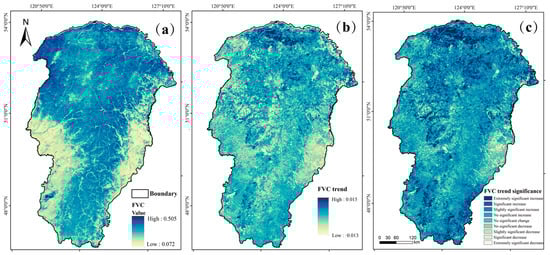
Figure 3.
(a–c) Changes in FVC trends and significance test results from 2001 to 2022: (a) represents the spatial distribution of FVC; (b) represents the variation trend of FVC; (c) represents the significance test of FVC variation trend.
In summary, from 2001 to 2022, FVC in the Greater Khingan Mountains region demonstrated an overall increasing trend, with notable spatial variations. The vegetation recovery was more pronounced in the southern and eastern regions, whereas certain areas still experienced a declining trend.
3.2. Global Results
3.2.1. Model Comparison
The models’ performance was assessed using statistical metrics, including R2, RMSE, MAE, and MSE. As shown in Table 5, the XGeoML model outperformed the other models across all evaluation parameters. This finding suggests that the XGeoML model is well-suited to identifying the driving factors of FVC in the Greater Khingan Mountains.
Table 5.
Parameter performance of OLS, GWR, RF, and XGeoML models.
3.2.2. Global Relative Importance Influence Analysis of Driving Factors on FVC
The XGeoML model was used to compute the absolute Shapley values (|SHAP|) for all samples, quantifying the overall impact of each driving factor on the spatial differentiation of FVC. Figure 4a presents the global feature importance, which considers all samples and calculates the mean |SHAP| value for each driving factor. Among all selected factors, elevation had the greatest influence on the spatial differentiation of the FVC, with a mean |SHAP| value of 0.011, indicating that elevation was the dominant factor affecting the spatial distribution of FVC. This was followed by POP (0.007), GDP (0.006), and slope (0.005). The effects of MAT, MAP, TMIN, TMAX, soil type, and aspect were relatively similar, whereas nighttime light had the lowest mean |SHAP| value, suggesting its minimal impact on spatial variation in FVC.
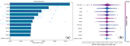
Figure 4.
(a,b) Global and local importance of drivers: (a) represents the global feature importance; (b) represents the local feature importance.
Figure 4b illustrates the local feature importance by plotting the Shapley values of each sample for each feature, where the y-axis represents the driving factors and the x-axis represents the SHAP values. A value greater than 0 indicates a positive influence, while a value less than 0 indicates a negative influence. The local feature importance analysis (Figure 4b) revealed that elevation, POP, GDP, slope, soil type, TMIN, and aspect generally had a positive effect on spatial variation in the FVC, meaning that an increase in these factors was typically associated with higher FVC values. In contrast, factors such as the MAT and the MAP exhibited a weak positive impact on FVC, whereas nighttime light showed no significant influence on the spatial differentiation of FVC.
3.2.3. Nonlinear and Threshold Influence Analysis of Driving Factors on FVC
Local dependence plots (LDPs) and SHAP values were used to reveal the nonlinear and threshold effects of driving factors on the spatial differentiation of FVC in the Greater Khingan Mountains (Figure 5).
Figure 5.
The local dependence of the driving factors behind FVC: red line represents variation trend.
The impact of elevation on FVC exhibited a distinct nonlinear relationship with a threshold effect, forming an inverted U-shape. When the elevation ranged from 200 to 600 m, the SHAP values increased significantly, indicating that this elevation range was favorable for vegetation growth. When the elevation exceeded 500 m, the SHAP values transitioned from negative to positive, suggesting a local effect shift in how elevation influences vegetation growth. The SHAP value peaked at around 600 m, highlighting the strongest positive impact of elevation on FVC at this point. However, as the elevation continued to increase, the SHAP values gradually declined, turning negative at approximately 1200 m, indicating that high elevations may suppress vegetation growth. The slope generally exhibited a relatively stable positive effect on FVC below 26°, meaning that an increase in slope was typically associated with higher FVC values. Aspect influenced FVC by affecting soil moisture and the distribution of solar radiation. In the study area, when the aspect ranged between 50° and 150°, the SHAP values increased with aspect, likely due to favorable sunlight and moisture conditions that supported vegetation growth. However, when the aspect exceeded 225°, the SHAP values shifted from positive to negative, indicating that certain aspect orientations may have an adverse effect on FVC. The impact of soil type factors on FVC showed significant fluctuations in the SHAP values, suggesting complex spatial variations. This trend may be associated with differences in the soil’s physicochemical properties required by different types of vegetation.
In the study area, the influence of GDP and POP on FVC exhibited a nonlinear variation trend, with their SHAP values showing a “decline-followed-by-rise” pattern. As economic activity and population growth intensified, land development and urban expansion likely exerted negative impacts on FVC, leading to lower SHAP values. The SHAP values for the nighttime light factor were predominantly zero, likely due to the low level of urbanization in the Greater Khingan Mountains. Limited nighttime light pollution and minimal direct urban disturbances contributed to the weak influence of urbanization on vegetation growth. Furthermore, as the region is primarily covered by forest ecosystems, the spatial extent of nighttime lighting is restricted, resulting in an insignificant impact on FVC.
The SHAP values for MAT showed no significant overall variation. However, when the MAT exceeded the 0 °C threshold, the direction of the changes in the SHAP values shifted slightly toward a positive influence. This trend suggests that temperatures rising above freezing benefits vegetation growth, likely because the suppression of photosynthesis and metabolic activities due to low temperatures diminishes, thereby promoting an increase in FVC. The SHAP values for TMAX gradually decreased as the maximum temperature increased, indicating that excessively high maximum temperatures may suppress FVC. This effect is likely related to drought stress induced by high temperatures. In contrast, TMIN exhibited a positive effect on FVC, with the SHAP values increasing as the minimum temperature rose. This pattern suggests that higher minimum temperatures help reduce the risk of nighttime frost damage, creating a more stable growth environment for vegetation. FVC’s response to MAP demonstrated a clear threshold effect. When the MAP ranged between 350 and 500 mm, the SHAP values were positive, indicating that moderate precipitation levels promote vegetation growth. However, when the precipitation dropped below 350 mm or exceeded 500 mm, the SHAP values turned negative. This pattern suggests that both insufficient and excessive rainfall can negatively impact vegetation, likely due to water stress or excessive waterlogging.
3.2.4. Interaction Effects of Driving Factors on FVC
Quantifying the effects of individual driving factors was insufficient to fully reveal the mechanisms underlying the spatial differentiation of FVC. Therefore, it was necessary to investigate the synergistic effects among multiple factors and their combined influence on the spatial pattern of FVC further. Figure 6 shows the interaction effects between the driving factors calculated using the SHAP algorithm. The interaction effects revealed by SHAP represented the additional impact on the spatial variation in FVC resulting from the joint contribution of two driving factors, excluding their individual main effects. Nighttime light exhibited no significant interaction with the other variables, suggesting that this factor had a very limited contribution to the spatial differentiation of FVC when acting in combination with others and demonstrated a high degree of independence. In contrast, the interaction between elevation and slope was the strongest, indicating a possible synergistic mechanism between these two topographic factors in regulating hydrothermal conditions which played a key role in the vegetation distribution. In addition, a strong interaction was observed between POP and GDP, suggesting that socioeconomic factors associated with the intensity of human activity also exerted a notable impact on FVC when acting together. Overall, aside from nighttime light, most of the driving factors showed strong interaction effects with elevation. For instance, the interaction between elevation and POP was prominent, possibly reflecting the indirect regulatory effect of human activities on the vegetation cover across different altitudinal gradients. These results further confirmed the dominant role of elevation in driving the spatial variation in FVC in the study area.
Figure 6.
The interactions between driving factors behind FVC’s spatial differentiation. The position of each point indicates the strength of the interaction, while the density and spread of the points reflects the extent to which the interaction between two factors influence FVC variation. Each point corresponds to a sample, and its color coding is related to the feature value: the closer the color is to red, the greater the corresponding feature value of that sample; the more it leans towards blue.
3.3. Primary Factors Influencing FVC Identified at the Local Scale
To analyze the dominant effects of the driving factors at the local scale further, this study statistically analyzed the SHAP values for the driving factors at the county scale. Figure 7 shows the spatial distributions and area proportions for each dominant factor.
Figure 7.
(a–h) The spatial distributions of the main effects of the driving factors: (a) represents the spatial distribution of dominant factors among the total driving factors; (b) represents the spatial distribution of dominant factors among human driving factors; (c) represents the spatial distribution of dominant factors among climate driving factors; (d) represents the spatial distribution of dominant factors among landform driving factors; (e) represents the area proportion of dominant factors among all driving factors; (f) represents the area proportion of dominant factors among human driving factors; (g) represents the area proportion of dominant factors among climate driving factors; and (h) represents the area proportion of dominant factors among landform driving factors.
- (1)
- The local dominant effects of overall driving factors: Among all driving factors, elevation, GDP, POP, and soil type exhibited the strongest local dominant effects. Elevation had the most significant local dominant effect on the spatial differentiation of FVC in the Greater Khingan Mountains, covering 63.2% of the study area, mainly concentrated in 12 counties, including Genhe City, Ergun County, and Huma County (Figure 7a). These areas are characterized by mountainous and high-elevation terrain, with significant topographic variation leading to substantial differences in vegetation type and distribution. POP was the second most influential local driving factor, covering 21.1% of the study area (Figure 7e), mainly in Tahe County, Morin Dawa Daur Autonomous Banner, and Ewenki Autonomous Banner (Figure 7a).
- (2)
- The local dominant effects of different driving factors: Of the human drivers, POP and GDP had the strongest local dominant effects. POP had the widest range of influence (Figure 7f), covering 74% of the study area, where the population density is relatively high and human activities are frequent. This indicates that changes in POP may be an important factor affecting FVC. GDP had localized effects mainly in Mohe City, Ergun City, and Huma County (Figure 7b), where economic activities such as agriculture and tourism have led to land use changes, thereby impacting FVC. For instance, tourism development in Mohe City and Ergun City might have caused ecological changes in these regions. Climate drivers had dominant effects in different counties, among which the dominant effect of MAP covered 47.4% of the study area, mainly the southern part of the region (Figure 7g). This suggests that FVC changes in these areas may be closely related to water availability. MAT, TMIN, and TMAX had local dominant effects on the northern part of the study area (Figure 7c), likely due to the extremely cold climate in this region, where the vegetation is more sensitive to temperature fluctuations. For example, Genhe City, known as “China’s Cold Pole”, has recorded extreme winter temperatures as low as −58 °C. In the landform drivers, elevation had the most significant local dominant effect, covering 74% of the study area (Figure 7h). This effect was mainly distributed in the high-elevation areas of the Greater Khingan Mountains, where the rugged topography made the vegetation and FVC highly sensitive to changes in elevation. Soil type had a certain dominant effect in some plain areas, such as New Barag Left Banner, suggesting that soil type is a key factor influencing changes in FVC in these regions (Figure 7d).
4. Discussion
4.1. The Advantages of the KNDVI-XGeoML Framework
This study developed a KNDVI-XGeoML coupled framework, integrating nonlinear vegetation index optimization with spatially interpretable machine learning to simultaneously enhance the retrieval accuracy for FVC and improve the analysis of its driving mechanisms. In investigating the spatial differentiation of FVC drivers, this study quantified the nonlinear relationships and the threshold effects of human drivers, climate drivers, and landform drivers on changes in FVC, offering an advantage over the traditional linear models [21]. Compared with the global nonlinear fitting methods of the traditional machine learning models, the XGeoML model employed in this study integrated the spatial weighting method of GWR and the nonlinear fitting capability of machine learning to construct multiple localized nonlinear models, considering the effects of spatial autocorrelation between FVC and its driving factors. This improvement compensated for the limitations of traditional machine learning models in ignoring spatial dependencies among variables and enhanced its ability to identify key driving factors [45]. In addition, XGeoML combined with the SHAP method enhanced the interpretability of the model. This integration not only quantified the global and local impacts of human activities, climate, and landform drivers on variations in FVC but also unveiled the mechanisms of the driving factors in different regions. By mitigating the black-box effect inherent in machine learning models, this approach enhanced the transparency and reliability of the results [46]. Furthermore, the results from the model comparison demonstrated that the KNDVI-XGeoML framework exhibited distinct advantages in analyzing the spatiotemporal dynamics compared to traditional models such as OLS, GWR, MGWR, LightGBM, GBR, and RF. For instance, in the FVC retrieval experiments, the XGeoML model achieved an R2 value of 0.777, outperforming the GWR model (R2 = 0.705) and thereby significantly improving the model’s accuracy in identifying driving factors.
In summary, this framework realized an end-to-end optimization process from FVC retrieval to the driving mechanism analysis, providing robust scientific support for ecosystem management and policy decision-making. Overall, the construction of the KNDVI-XGeoML coupled framework offered a novel methodological approach to FVC retrieval and ecological driver analysis while also serving as a valuable tool for regional ecosystem management and sustainability planning.
4.2. Spatiotemporal Trends in FVC
From 2001 to 2022, FVC in the Greater Khingan Mountains showed an overall increasing trend. Spatially, high FVC values were mainly concentrated in the northern and central parts of the study area, exhibiting significant spatial heterogeneity. This conclusion was consistent with the findings of Shi et al. [47], Gong [48], and Huang et al. [49]. This trend was primarily attributed to a series of ecological protection policies implemented by the government, particularly those aimed at forest conservation and vegetation restoration. For example, the Natural Forest Protection Program (NFPP), launched in 2000, strictly limited commercial logging activities and promoted natural forest recovery and ecological balance, thereby driving FVC growth [50]. Additionally, the Grain for Green Program (GFGP), introduced in 2001, not only facilitated the conversion of farmland into forested land but also expanded forest areas through afforestation efforts. The combined effects of these policies have steadily increased the forest FVC in the Greater Khingan Mountains. To validate this conclusion, this study applied a land use transition matrix analysis (Figure 8), which showed that the forested area in the Greater Khingan Mountains increased by 4003.76 km2 from 2001 to 2022. This result further confirmed the significant effectiveness of the aforementioned ecological protection policies. Thus, government-led ecological projects have played a crucial role in promoting forest vegetation restoration, providing a solid foundation for regional ecological improvements.
Figure 8.
The land use transfer matrix for the Greater Khingan Mountains.
4.3. Driving Factors of the Spatial Differentiation in FVC
The global and local results of the SHAP analysis indicated that among the landform drivers, elevation was the most significant factor influencing the spatial variation in FVC in the Greater Khingan Mountains. Specifically, the response of FVC to elevation exhibited a distinct nonlinear pattern: when the elevation was below 600 m, FVC gradually increased with increasing elevation; however, beyond 600 m, FVC progressively decreased as the elevation rose, although it remained higher than that in low-elevation areas. This finding aligned with the terrain threshold effect reported by Gao et al. [51]. Previous studies have demonstrated that spatial variation in FVC is a result of multiple factors interacting [52], and the spatial distribution of the driving factors, along with their SHAP values, further revealed the interactions between elevation and the other drivers. In particular, the human activity factors (POP and GDP) exhibited significant differences across elevations. In the high-elevation regions, both the POP and GDP were relatively low, with correspondingly lower SHAP values. This suggested that high elevation acted as a natural barrier to human activities, thereby mitigating their negative impact on FVC [53,54]. Additionally, prior research has shown that elevation indirectly influences FVC by affecting the environmental conditions for vegetation growth, a finding consistent with our results [55]. Further analysis of the spatial distribution of the driving factors revealed that in the higher-elevation regions, MAT, TMAX, TMIN, and MAP were all at moderate levels. This suggested that elevation may have influenced FVC indirectly by modulating climate factors. Among the landform drivers, aside from elevation, slope was identified as the second most influential factor affecting the spatial variation in FVC. When the slope was less than 4°, the FVC was generally low; however, the FVC showed a gradual increasing trend within the slope range of 8° to 26°. The spatial distributions of the driving factors (Figure 9) indicated that slope was closely related to elevation, with high-slope areas often corresponding to higher elevations. Meanwhile, the interaction analysis in Section 3.2.4 further confirmed that a significant interaction existed between slope and elevation. Their synergistic effect was an important driver of the spatial heterogeneity in FVC. This suggested that slope not only directly affected vegetation growth but also indirectly influenced vegetation coverage by regulating elevation and other environmental factors, such as soil moisture and nutrient conditions. Based on this, it was inferred that the relatively lower FVC in areas with slopes of less than 4° was mainly due to the relatively flat terrain providing favorable conditions for human activities, which increased the land use intensity and thereby limited the growth of natural vegetation. In contrast, areas with slopes between 8° and 26° experienced less human disturbance, partly because of the steeper slopes, combined with higher elevation. Additionally, the terrain within this slope range was conducive to retaining soil moisture and accumulating nutrients, creating more suitable ecological conditions for vegetation growth, thus resulting in relatively higher FVC values [54]. By comparison, aspect had a relatively minor overall impact on FVC, particularly when contrasted with elevation and slope. However, differences across aspects were still observed, which was consistent with previous findings [56]. For instance, southeast-facing slopes exhibited the highest FVC values. This may have been due to variations in the soil moisture and exposure to solar radiation across different aspects, which in turn influenced vegetation growth [57]. Therefore, future studies should integrate solar radiation and soil moisture data to elucidate further the mechanisms through which aspect drives the spatial variation in the FVC in the Greater Khingan Mountains.
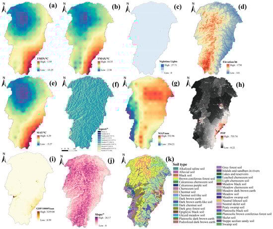
Figure 9.
The spatial distributions of FVC drivers: (a) represents the spatial distribution of TMIN; (b) represents the spatial distribution of TMAX; (c) represents the spatial distribution of nighttime light; (d) represents the spatial distribution of elevation; (e) represents the spatial distribution of MAT; (f) represents the spatial distribution of aspect; (g) represents the spatial distribution of MAP; (h) represents the spatial distribution of POP; (i) represents the spatial distribution of GDP; (j) represents the spatial distribution of slope; and (k) represents the spatial distribution of soil type.
POP and GDP were identified as key driving factors influencing the spatial variation in FVC. The variation trend in their SHAP values suggested a nonlinear negative impact on FVC, characterized by an initial intensification followed by a subsequent weakening. This trend likely reflected the dual effects of human activities on the FVC at different stages. In regions with a low population density and weak economic activity, human disturbances were minimal, and ecosystems remained relatively stable, allowing FVC to be maintained at a higher level. However, as the POP and GDP increased, the intensity of human activities—such as deforestation, land development, and infrastructure expansion—escalated, leading to a decline in FVC. Notably, in areas with a high POP and GDP, despite frequent human activities, these regions often exhibited greater environmental awareness and were subject to stricter ecological restoration and sustainable development policies. Initiatives such as urban greening programs and ecological restoration projects implemented by governments contributed to the recovery of FVC. This suggested that appropriate environmental governance measures could effectively mitigate the negative impact of human activities on FVC [58].
The dominant effects of the temperature-related factors (MAT, TMAX, and TMIN) and MAP on FVC were roughly equivalent (Figure 7). Furthermore, the spatial distribution of these climate drivers, as illustrated in Figure 9, revealed significant spatial heterogeneity in MAT, TMAX, TMIN, and MAP. This implied that climate factors influenced FVC by shaping distinct water–heat combinations across different vegetation types. Specifically, the adaptability and growth conditions of the vegetation in different regions were likely determined by their respective hydrothermal mode, ultimately leading to spatial variations in the FVC. Therefore, climate factors not only directly affected vegetation growth but also indirectly shaped the FVC distribution patterns by regulating the water–heat balance across different regions.
4.4. Policy Recommendations for Ecological Security Barrier Construction
Figure 10 shows the spatial distributions of the SHAP values for the drivers of FVC. Based on the influence of the dominant FVC drivers across different counties, this study established natural-environment-dominated zones and human-activity-dominated zones. Implementing refined zoning management strategies tailored to the local conditions aimed to support the formulation of scientific policies that would promote sustained regional growth in FVC, long-term ecological stability, and sustainable development.
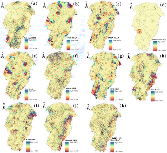
Figure 10.
Spatial distributions of SHAP values for FVC drivers: (a) represents the spatial distribution of the SHAP values for soil type; (b) represents the spatial distribution of the SHAP values for TMIN; (c) represents the spatial distribution of the SHAP values for TMAX; (d) represents the spatial distribution of the SHAP values for nighttime light; (e) represents the spatial distribution of the SHAP values for MAT; (f) represents the spatial distribution of the SHAP values for aspect; (g) represents the spatial distribution of the SHAP values for MAP; (h) represents the spatial distribution of the SHAP values for POP; (i) represents the spatial distribution of the SHAP values for GDP; (j) represents the spatial distribution of the SHAP values for elevation; and (k) represents the spatial distribution of the SHAP values for slope.
- (1)
- Natural-environment-dominated zones: The natural-environment-dominated zone areas accounted for 73.6% of the study area. The dominant effect of elevation on the FVC showed both positive and negative spatial differentiation across different counties. Specifically, in Ergun City, Chen Barag Banner, Hailar District, Yakeshi City, and Horqin Right Front Banner, elevation had a positive effect on the spatial variation in FVC. The average elevation in these areas ranged from 650 to 900 m, and they were less influenced by human activities. The moderate terrain provided favorable water–heat conditions and ecological stability, which contributed to vegetation growth. Therefore, in the construction of ecological barriers in these counties, the threshold effect of elevation should be fully considered. A low-elevation transition zone (200–500 m) and a mid-elevation core zone (500–600 m) should be defined, with human activity buffer zones established in the transition areas. Strict restrictions on the construction of tourism facilities and the expansion of arable land ought to be implemented to minimize human interference and maintain the positive effect of elevation on FVC. In contrast, in Jiagedaqi District, Huma County, Arong Arun Banner, Genhe City, Jalaid Banner, Oroqen Autonomous Banner, and Zhalantun City, elevation showed a negative effect on the spatial variation in FVC. In areas with lower elevation (e.g., Jiagedaqi District, with an average elevation of 483 m), the urban expansion and economic activities had significantly suppressed vegetation growth. In higher-elevation areas, negative effects stemmed from uneven water–heat conditions which restricted vegetation growth [59]. Therefore, in these counties, urban expansion should be controlled to reduce its impact on FVC by delineating ecological red lines, optimizing the land use management, and strictly protecting forest resources. Additionally, optimizing the vegetation structures in high-elevation areas could improve the cold and drought resistance of ecosystems—such as promoting cold- and drought-resistant tree species and increasing the proportion of mixed coniferous and broadleaf forests—which would enhance ecosystem stability and resilience. At the same time, climate-adaptive management should be strengthened, a long-term ecological monitoring system should be established, and extreme weather events should be closely monitored to ensure stable vegetation restoration. The influence of soil type on FVC cannot be overlooked. In particular, Arxan City exhibited a positive dominant effect of the soil type on FVC, likely due to its high soil fertility and optimal pH levels, which provided essential nutrients and favorable conditions for plant growth [60]. Additionally, soil type influences microbial diversity and activity, further contributing to vegetation development [61]. Given these drivers, future vegetation restoration initiatives—such as afforestation and grassland restoration—should prioritize areas with suitable soil types. Moreover, establishing a long-term monitoring system to examine the relationship between soil properties and FVC would provide valuable scientific insights for policy formulation. To safeguard these high-quality soil resources, relevant laws and regulations should be enacted to prevent soil degradation. Conversely, in New Barag Left Banner, soil type exerted a dominant negative effect on FVC, suggesting that unfavorable soil conditions hindered vegetation growth. Consequently, future ecological barrier construction in this region should focus on soil improvement strategies. Measures such as applying organic amendments and soil conditioners could enhance the soil’s structure and fertility, ultimately promoting vegetation recovery.
- (2)
- Human-activity-dominated zones: Human-activity-dominated zones accounted for 26.4% of the study area. GDP and POP served as the dominant drivers of the FVC in some regions, showing distinct spatial distribution patterns. One area where the GDP played a dominant role was Mohe City. In this region, GDP had a negative dominant effect on FVC. This indicates that human economic activities had negatively impacted FVC. Mohe City is a well-known tourist destination in China, often referred to as the “Arctic of China”. Its booming tourism industry has led to the expansion of tourism infrastructure, such as road construction, which might place pressure on vegetation. Therefore, future ecological barrier construction in this area should focus on sustainable tourism management. This includes developing eco-friendly tourism plans, raising tourists’ awareness about environmental protection, and limiting tourism capacity. These measures aim to prevent over-tourism from damaging the ecological environment. Additionally, tourism infrastructure development should adopt Low-Impact Development (LID) practices to minimize the damage to vegetation. Legislation should also be strengthened to protect ecosystems, imposing strict penalties for actions that harm vegetation, while exploring green economic models to achieve a balance between economic development and ecological restoration. On the other hand, POP emerged as the dominant negative factor affecting FVC in Morin Dawa Daur Autonomous Banner, Ewenki Autonomous Banner, and Tahe County. As illustrated in Figure 9, these three regions exhibited higher population densities, which correlated with increased human disturbance and vegetation degradation [62]. To address this issue, ecological protection policies should be implemented to strictly regulate land development, minimizing the unnecessary destruction of vegetation. Additionally, raising public awareness about environmental conservation; encouraging community participation in reforestation and vegetation restoration initiatives; and establishing green buffer zones around urban areas would be essential in mitigating human-induced ecological stress. By integrating these measures, it might be possible to achieve a sustainable balance between economic development and environmental protection, ensuring long-term ecosystem stability while fostering economic resilience.
4.5. Research Limitations and Future Directions
Although the KNDVI-XGeoML coupling framework constructed in this study provided significant insights into the spatial evolution of FVC and its driving mechanisms in the Greater Khingan Mountains, certain limitations remained that should not be overlooked. This study primarily focused on the spatial differentiation in the annual average FVC from 2001 to 2022, revealing the effects of driving factors in the spatial dimension. However, it did not fully account for the temporal dynamic variations in these mechanisms. Consequently, the time-lagged effects of certain drivers and key turning points in the long-term trends might have been overlooked. For instance, extreme climatic events could have induced short-term fluctuations in FVC, yet these impacts might have been masked when the data were averaged annually. Understanding how climatic variability and anthropogenic influences affect the FVC dynamics across multiple temporal scales—seasonal, interannual, and decadal—is essential for a comprehensive assessment of vegetation changes. Future research should focus on incorporating multiscale temporal analyses and investigating the potential time-lagged and nonlinear responses of vegetation to environmental drivers.
5. Conclusions
This study constructed a KNDVI-XGeoML coupled framework, integrating the TS and MK methods to systematically reveal the spatiotemporal evolution characteristics of FVC in the Greater Khingan Mountains region of China from 2001 to 2022, as well as the driving mechanisms behind its spatial differentiation. (1) Past ecological policies in the Greater Khingan Mountains region have effectively promoted vegetation restoration. From 2001 to 2022, FVC exhibited an overall increasing trend. (2) The XGeoML model demonstrated high applicability to analyses of the spatial heterogeneity of FVC. Compared with the traditional models, the XGeoML model significantly improved the recognition ability of FVC’s driving factors; effectively quantified the nonlinear and threshold effects between FVC and its drivers; and solved the “black-box” problem of the traditional machine learning models. (3) Except for nighttime light, all of the selected driving factors exhibited nonlinear and threshold effects on FVC, with elevation exerting the most significant impact. (4) The dominant influencing factors for FVC varied across different regions of the Greater Khingan Mountains. In the northern alpine areas (Tahe County and Mohe City), FVC was primarily influenced by POP and GDP, whereas in the southern region (Arxan City and New Barag Left Banner), soil type properties played a dominant role. (5) Based on the spatial distribution of the dominant influencing factors, this study divided the region into natural-environment-dominated zones and human-activity-dominated zones, which accounted for 73.6% and 26.4% of the study area, respectively. In the future, ecological barrier construction in the Greater Khingan Mountains region should adopt differentiated ecological management strategies aligned with the dominant influencing factors in order to enhance the precision and effectiveness of ecological restoration efforts.
Author Contributions
Conceptualization: Z.W. and B.W.; methodology: Z.W. and B.W.; software, Z.W.; validation: Z.W. and B.W.; formal analysis: Z.W.; investigation: Z.W.; resources: Z.W.; data curation: Z.W.; writing—original draft preparation: Z.W. and B.W.; writing—review and editing: B.W., Z.W., and C.L.; visualization: Z.W. and B.W.; supervision: B.W., Q.Z., and C.L.; project administration: Q.Z.; funding acquisition: B.W. and C.L. All authors have read and agreed to the published version of the manuscript.
Funding
This work was supported by the National Key R&D Program of China (2023YFF1304002); the Key R&D Program of Inner Mongolia, China (2023YFDZ0026); the Inner Mongolia Natural Science Foundation, China (2025MS03014); the Forestry Discipline Self-Established Research Projects of Inner Mongolia Agricultural University, China (LX20250625-10); and the Research Team Construction Project of Forestry College, Inner Mongolia Agricultural University, China.
Data Availability Statement
The original contributions presented in this study are included in the article. Further inquiries can be directed to the corresponding author.
Conflicts of Interest
The authors declare no conflicts of interest.
References
- Zhang, R.; Lou, C.D.; Zhang, Z.T.; Huang, X.R.; Xie, J.; Hao, Q.J.; Zhang, L.B.; Li, Y.H.; Liu, X.L. Utilization and protection of water resources under the background of carbon neutralization. Adv. Eng. Sci. 2022, 54, 69–82. [Google Scholar]
- Yi, S. Analysis Vegetation Coverage Changes in Karst Area on RS and GIS-Luota in Human Province as an Example. Master’s Thesis, Guangxi Normal University, Guilin, China, 2008. [Google Scholar]
- Zheng, K.Y.; Tan, L.S.; Sun, Y.W.; Wu, Y.J.; Duan, Z.; Xu, Y.; Gao, C. Impacts of climate change and anthropogenic activities on vegetation change: Evidence from typical areas in China. Ecol. Indic. 2021, 126, 107648. [Google Scholar] [CrossRef]
- Wang, C.; Hou, P.; Liu, X.M.; Yuan, J.F.; Zhou, Q.; Lü, N. Spatio-temporal changes in vegetation cover of the national key ecosystem protection and restoration project areas, China. Acta Ecol. Sin. 2023, 43, 8903–8916. [Google Scholar]
- Li, M.Y.; Liu, T.X.; Luo, Y.Y.; Duan, L.M.; Ma, L.; Wang, Y.X.; Zhang, J.Y.; Zhou, Y.J.; Yang, L.; Chen, Z.X. Fractional vegetation coverage downscaling inversion method based on Land Remote-Sensing Satellite (System, Landsat-8) and polarization decomposition of Radarsat-2. Int. J. Remote Sens. 2021, 42, 3255–3276. [Google Scholar] [CrossRef]
- Li, Z.C.; Dong, G.T.; Yao, N. Analysis of spatiotemporal variations and driving forces of NDVI in the middle reaches of Yellow River during 1982–2015. Res. Soil Water Conserv. 2024, 31, 202–210. [Google Scholar]
- Jia, K.; Yao, Y.J.; Wei, X.Q.; Gao, S.; Jiang, B.; Zhao, X. A review on fractional vegetation cover estimation using remote sensing. Adv. Earth Sci. 2013, 28, 774–782. [Google Scholar]
- Cheng, H.F.; Zhang, W.B.; Chen, F. Advances in researches on application of remote sensing method to estimating vegetation coverage. Remote Sens. Land Resour. 2008, 57, 13–18. [Google Scholar]
- Zhou, L.M.; Tucker, C.J.; Kaufmann, R.K.; Slayback, D.; Shabanov, N.V.; Myneni, R.B. Variations in northern vegetation activity inferred from satellite data of vegetation index during 1981 to 1999. J. Geophys. Res. Atmos. 2001, 106, 20069–20083. [Google Scholar] [CrossRef]
- Wilson, A.D.; Abraham, N.A.; Barratt, R.; Choate, J.; Green, D.R.; Harland, R.J.; Oxley, R.E.; Stanley, R.J. Evaluation of methods of assessing vegetation change in the semi-arid rangelands of southern Australia. Rangeland J. 1987, 9, 5–13. [Google Scholar] [CrossRef]
- Jamali, S.; Jönsson, P.; Eklundh, L.; Ardö, J.; Seaquist, J. Detecting changes in vegetation trends using time series segmentation. Remote Sens. Environ. 2015, 156, 182–195. [Google Scholar] [CrossRef]
- Li, M.M. The Method of Vegetation Fraction Estimation by Remote Sensing. Master’s Thesis, Chinese Academy of Sciences, Beijing, China, 2003. [Google Scholar]
- Mao, P.P.; Zhang, J.; Li, M.; Liu, Y.L.; Wang, X.; Yan, R.R.; Shen, B.B.; Zhang, X.; Shen, J.; Zhu, X.Y. Spatial and temporal variations in fractional vegetation cover and its driving factors in the Hulun Lake region. Ecol. Indic. 2022, 135, 108490. [Google Scholar] [CrossRef]
- Xu, J.L.; Yang, X.C.; Zhao, W.J.; Yang, Z.Q.; Zhong, Y.X.; Shi, L.Y.; Ma, P.F. Evolution characteristics of vegetation coverage in central and western Inner Mongolia under the background of climate change. Ecol. Environ. Sci. 2024, 33, 1008–1018. [Google Scholar] [CrossRef]
- Gao, X.; Huete, A.R.; Ni, W.G.; Miura, T. Optical–biophysical relationships of vegetation spectra without background contamination. Remote Sens. Environ. 2000, 74, 609–620. [Google Scholar] [CrossRef]
- Sellers, P.J. Canopy reflectance, photosynthesis and transpiration. Int. J. Remote Sens. 1985, 6, 1335–1372. [Google Scholar] [CrossRef]
- Zeng, X.B.; Dickinson, R.E.; Walker, A.; Shaikh, M.; DeFries, R.S.; Qi, J.G. Derivation and evaluation of global 1-km fractional vegetation cover data for land modeling. J. Appl. Meteorol. 2000, 39, 826–839. [Google Scholar] [CrossRef]
- Camps-Valls, G.; Campos-Taberner, M.; Moreno-Martínez, Á.; Walther, S.; Duveiller, G.; Cescatti, A.; Mahecha, M.D.; Muñoz-Marí, J.; García-Haro, F.J.; Guanter, L. A unified vegetation index for quantifying the terrestrial biosphere. Sci. Adv. 2021, 7, 7447. [Google Scholar] [CrossRef] [PubMed]
- Wang, Q.; Moreno-Martínez, Á.; Muñoz-Marí, J.; Campos-Taberner, M.; Camps-Valls, G. Estimation of vegetation traits with kernel NDVI. ISPRS J. Photogramm. Remote Sens. 2023, 195, 408–417. [Google Scholar] [CrossRef]
- Liu, Y.; Huang, T.T.; Qiu, Z.Y.; Guan, Z.L.; Ma, X.Y. Effects of precipitation changes on fractional vegetation cover in the Jinghe River basin from 1998 to 2019. Ecol. Inform. 2024, 80, 102505. [Google Scholar] [CrossRef]
- Liu, Z.P.; Zhang, Y.S. Vegetation cover change and its response to human activities in the southwestern karst region of China. Front. Ecol. Evol. 2024, 12, 1326601. [Google Scholar] [CrossRef]
- Tuoku, L.; Wu, Z.J.; Men, B.H. Impacts of climate factors and human activities on NDVI change in China. Ecol. Inform. 2024, 81, 102555. [Google Scholar] [CrossRef]
- Ming, Y.J.; Liu, Y.; Li, Y.P.; Song, Y.Z. Unraveling nonlinear and spatial non-stationary effects of urban form on surface urban heat islands using explainable spatial machine learning. Comput. Environ. Urban Syst. 2024, 114, 102200. [Google Scholar] [CrossRef]
- Georganos, S.; Grippa, T.; Niang Gadiaga, A.; Linard, C.; Lennert, M.; Vanhuysse, S.; Mboga, N.; Wolff, E.; Kalogirou, S. Geographical random forests: A spatial extension of the random forest algorithm to address spatial heterogeneity in remote sensing and population modelling. Geocarto Int. 2021, 36, 121–136. [Google Scholar] [CrossRef]
- Li, Z.Q. Extracting spatial effects from machine learning model using local interpretation method: An example of SHAP and XGBoost. Comput. Environ. Urban Syst. 2022, 96, 101845. [Google Scholar] [CrossRef]
- Grekousis, G.; Feng, Z.X.; Marakakis, I.; Lu, Y.; Wang, R.Y. Ranking the importance of demographic, socioeconomic, and underlying health factors on US COVID-19 deaths: A geographical random forest approach. Health Place 2022, 74, 102744. [Google Scholar] [CrossRef] [PubMed]
- Xiang, Y.; Huang, C.B.; Huang, X.; Zhou, Z.X.; Wang, X.S. Seasonal variations of the dominant factors for spatial heterogeneity and time inconsistency of land surface temperature in an urban agglomeration of central China. Sustain. Cities Soc. 2021, 75, 103285. [Google Scholar] [CrossRef]
- Liu, L.B. An ensemble framework for explainable geospatial machine learning models. Int. J. Appl. Earth Obs. Geoinf. 2024, 132, 104036. [Google Scholar] [CrossRef]
- Bansal, P.; Quan, S.J. Examining temporally varying nonlinear effects of urban form on urban heat island using explainable machine learning: A case of Seoul. Build. Environ. 2024, 247, 110957. [Google Scholar] [CrossRef]
- Qi, L.; Zhang, Y.; Xu, D.; Zhu, Q.; Zhou, W.M.; Zhou, L.; Wang, Q.W.; Yu, D.P. Trade-offs and synergies of ecosystem services in forest barrier belt of Northeast China. Chin. J. Ecol. 2021, 40, 3401–3411. [Google Scholar] [CrossRef]
- Zhu, J.J.; Zhang, Q.L.; Wang, A.Z.; Wang, C.K.; Yu, L.Z.; Yu, D.P.; Zhang, Q.Z.; Yan, Q.L.; Zheng, X.B.; Wang, B.; et al. Suggestions for improving the qualities and functions of forest ecosystems in northeast China. Terrest. Ecosyst. Conserv. 2022, 2, 41–48. [Google Scholar]
- Yu, D.P.; Zhou, L.; Zhou, W.M.; Ding, H.; Wang, Q.W.; Wang, Y.; Wu, X.Q.; Dai, L.M. Forest management in Northeast China: History, problems, and challenges. Environ. Manag. 2011, 48, 1122–1135. [Google Scholar] [CrossRef]
- Wang, Z.R.; Miao, W.H.; Hu, R.C.; Gao, M.L.; Liu, L.; Li, Y.; Fu, Y.; Sarula, L. Driving forces of herbaceous species diversity in natural forests in Northern Greater Khingan Mountains based on structural equation model. J. Northw. For. Univ. 2024, 39, 13–20. [Google Scholar]
- Cui, X.; Liang, T.G.; Liu, Y. Modeling of aboveground biomass of grassland using remotely sensed MOD09GA data. J. Lanzhou Univ. (Nat. Sci.) 2009, 45, 79–87. [Google Scholar] [CrossRef]
- Wang, R.; Ding, X.; Yi, B.J.; Wang, J.L. Spatiotemporal characteristics of vegetation cover change in the Central Yunnan urban agglomeration from 2000 to 2020 based on Landsat data and its driving factors. Geocarto Int. 2024, 39, 2316643. [Google Scholar] [CrossRef]
- Burton, A.L. OLS (Linear) regression. Encycl. Res. Methods Criminol. Crim. Just. 2021, 2, 509–514. [Google Scholar]
- Wang, X.R.; Gong, J.Z.; Yu, F.Y. Mutual feedback relationships and mechanisms of ecosystem four regulating services in the greater bay area of Guangdong, Hongkong and Macao. J. Northw. For. Univ. 2024, 33, 1130–1141. [Google Scholar] [CrossRef]
- Fotheringham, A.S.; Yang, W.B.; Kang, W. Multiscale geographically weighted regression (MGWR). Ann. Am. Assoc. 2017, 107, 1247–1265. [Google Scholar] [CrossRef]
- Ke, G.L.; Meng, Q.; Finley, T.; Wang, T.F.; Chen, W.; Ma, W.D.; Ye, Q.W.; Liu, T.Y. Lightgbm: A highly efficient gradient boosting decision tree. Adv. Neural Inf. Process. Syst. 2017, 30, 3149–3157. [Google Scholar]
- Rigatti, S.J. Random forest. J. Insur. Med. 2017, 47, 31–39. [Google Scholar] [CrossRef]
- Su, J.; Nie, D.W.; Li, X.M.; Zhang, X.S.; Song, J.Z.; Dong, M.F. Research on the meteorological influencing factors of PM2.5 concentration in Guanzhong region based on CatBoost-SHAP-MCM model. Res. Environ. Sci. 2025, 38, 787–797. [Google Scholar]
- Prettenhofer, P.; Louppe, G. Gradient boosted regression trees in scikit-learn. In Proceedings of the PyData 2014, London, UK, 21–23 February 2014. [Google Scholar]
- Garreau, D.; Luxburg, U. Explaining the explainer: A first theoretical analysis of LIME. In Proceedings of the International Conference on Artificial Intelligence and Statistics, Online, 26–28 August 2020; pp. 1287–1296. [Google Scholar]
- Van den Broeck, G.; Lykov, A.; Schleich, M.; Suciu, D. On the tractability of SHAP explanations. J. Artif. Intell. Res. 2022, 74, 851–886. [Google Scholar] [CrossRef]
- Xiao, X.; Wang, Q.Z.; Guan, Q.Y.; Zhang, Z.P.; Yan, Y.; Mi, J.M.; Yang, E.Q. Quantifying the nonlinear response of vegetation greening to driving factors in Longnan of China based on machine learning algorithm. Ecol. Indic. 2023, 151, 110277. [Google Scholar] [CrossRef]
- Yuan, J.L.; Zhao, H.H.; Liu, X.H.; Li, H.Y.; Jiang, D.; Zhao, C.Y.; Xing, L.Y.; Luo, X.P.; Wang, R.; Wang, C. Driving force analysis and ecological assessment of spatiotemporal changes in vegetation cover in the Kunlun Mountains from 2000 to 2020. Geol. China 2024, 51, 1822–1838. [Google Scholar]
- Shi, S.; Li, W.; Lin, X.P.; Zhai, Y.C.; Ding, Y.S. Spatio-temporal variations of vegetation NDVI and influencing dactors in Heilongjiang province. Res. Soil Water Conserv. 2023, 30, 294–305. [Google Scholar]
- Gong, Z.Q. Analysis of Spatio-Temporal Variation Characteristics and Driving Mechanism of Vegetation Coverage in Daxing ‘an Mountain. Master’s Thesis, Inner Mongolia Agricultural University, Hohhot, China, 2023. [Google Scholar]
- Huang, Y.; Song, H.Q.; Hu, Q.; Wu, H.; Lu, J.Y.; Li, B.Y. Spatio-temporal dynamics of NDVI and its response to hydrothermal conditions in Inner Mongolia from 2000 to 2020. Res. Soil Water Conserv. 2024, 31, 197–204+213. [Google Scholar]
- Li, W.J.; Yang, J.Y.; Fu, B.; Zhao, Q.Y.; Tan, Z.; Guan, X. Spatial-temporal changes and prediction of carbon storage in Greater Khingan Mountains based on PLUS-InVEST model. J. Environ. Eng. Technol. 2024, 14, 1892–1904. [Google Scholar]
- Gao, F.F.; Xiang, Y.; Wang, S.Y.; Zhao, L.F.; Hou, M.; Bian, S.Y.; Luo, X. Analysis of vegetation change and driving factors in southeastern Tibet based on geographical detector and PLS-SEM. Environ. Sci. Technol. 2024, 47, 225–236. [Google Scholar] [CrossRef]
- He, H.C.; Ma, B.X.; Jing, J.L.; Xu, Y.; Dou, S.Q.; Liu, B. Spatio-temporal changes of NPP and natural factors in the Southwestern Karst Areas from 2000 to 2019. Res. Soil Water Conserv. 2022, 29, 172–178+188. [Google Scholar] [CrossRef]
- Zhang, Q.P.; Lu, H.E.; Zhao, D.C.; Zhuoma, L.C. Relationship between temporal and spatial changes of vegetation coverage and topographic factors in the Upper Yellow River in Gannan. Arid Zone Res. 2025, 42, 522–523. [Google Scholar]
- Gao, S.Q.; Dong, G.T.; Jiang, X.H.; Nie, T.; Yin, H.J.; Guo, X.W. Quantification of natural and anthropogenic driving forces of vegetation changes in the Three-River Headwater Region during 1982–2015 based on geographical detector model. Remote Sens. 2021, 13, 4175. [Google Scholar] [CrossRef]
- Rumpf, S.B.; Hülber, K.; Klonner, G.; Moser, D.; Schütz, M.; Wessely, J.; Willner, W.; Zimmermann, N.E.; Dullinger, S. Range dynamics of mountain plants decrease with elevation. Proc. Natl. Acad. Sci. 2018, 115, 1848–1853. [Google Scholar] [CrossRef]
- Nie, T.; Dong, G.T.; Jiang, X.H.; Lei, Y.X. Spatio-temporal changes and driving forces of vegetation coverage on the loess plateau of Northern Shaanxi. Remote Sens. 2021, 13, 613. [Google Scholar] [CrossRef]
- Duan, B.B. Correlation Between Leaf Traits and Leaf Water Use Efficiency Vein of Robinia Pseudoacacia in Different Aspects of Beishan Mountain in Lanzhou. Master’s Thesis, Northwest Normal University, Lanzhou, Chian, 2017. [Google Scholar]
- Yin, L.; Wei, W.; Li, H.R.; Xia, J.N.; Bo, L.M. Spatio-temporal differentiation and influencing factors of territorial spatial pattern evolution in China’s land area: A comparative analysis based on the Hu Huanyong Line and the Bole-Taipei Line. Geogr. Res. 2025, 44, 552–576. [Google Scholar]
- Hong, X.Q.; Sun, T.; Chen, L.D. Dynamic changes and driving factors of land surface phenology under the background of urbanization. Chin. J. Appl. Ecol. 2023, 34, 2436–2444. [Google Scholar]
- Du, Y.; Li, J.Z.; Niu, K.J.; Feng, P.; Hu, Q.; Zheng, Y. Analysis of vegetation change and its impact on natural runoff in the mountain area of the Yongding River Basin from 1982 to 2015. J. Hydraul. Eng. 2021, 52, 1309–1323. [Google Scholar]
- Mo, J.F.; Zhou, X.Y.; Mo, W.H.; Chen, Y.L. Analysis of vegetation ecological quality change and its driving forces in Guangxi from 2000 to 2020. Guihaia 2024, 44, 907–924. [Google Scholar]
- Hao, J.; Chen, X.Q.; Zhang, Z.; Gao, Y.; Li, L.Q.; Li, H.Y. Quantifying the temporal-spatial scale dependence of the driving mechanisms underlying vegetation coverage in coastal wetlands. Catena 2021, 204, 105435. [Google Scholar] [CrossRef]
Disclaimer/Publisher’s Note: The statements, opinions and data contained in all publications are solely those of the individual author(s) and contributor(s) and not of MDPI and/or the editor(s). MDPI and/or the editor(s) disclaim responsibility for any injury to people or property resulting from any ideas, methods, instructions or products referred to in the content. |
© 2025 by the authors. Licensee MDPI, Basel, Switzerland. This article is an open access article distributed under the terms and conditions of the Creative Commons Attribution (CC BY) license (https://creativecommons.org/licenses/by/4.0/).