Statistical Approach to Research on the Relationship Between Kp/Dst Geomagnetic Indices and Total GPS Position Error

Abstract

This study examines the impact of geomagnetic disturbances quantified by the Kp and Dst indices on the accuracy of single-frequency GPS positioning across mid-latitudes and the equatorial zone, with a focus on temporal and spatial positioning errors variability. GNSS data from a globally distributed network of 14 IGS stations were analyzed for September 2017, featuring significant geomagnetic activity. The selection of stations encompassed equatorial and mid-latitude regions (approximately ±45°), strategically aligned with the distribution of the Dst index during geomagnetic storms. Satellite navigation data were processed using RTKLIB software in standalone mode with standardized atmospheric and orbital corrections. The GPS was chosen over GLONASS following preliminary testing, which revealed a higher sensitivity of GPS positional accuracy to variations in geomagnetic indices such as Kp and Dst, despite generally lower total error magnitudes. The ECEF coordinate system calculates the total GPS error as the vector sum of deviations in the X, Y, and Z axes. Statistical evaluation was performed using One-Way Repeated Measures ANOVA to determine whether positional error variances across geomagnetic activity phases were significant. The results of the variance analysis confirm that the variation in the total GPS positioning error is non-random and can be attributed to the influence of geomagnetic storms. However, regression analysis reveals that the impact of geomagnetic storms (quantified by Kp and Dst) displays spatiotemporal variability, with no consistent correlation to GPS positioning error dynamics. The findings, as well as the developed methodology, have qualitative implications for GNSS-dependent operations in sensitive sectors such as navigation, timing services, and geospatial monitoring.

1. Introduction

The consequences of ionospheric irregularities (change in density structure) on the propagation of GNSS (Global Navigation Satellite System) signals are the subject of numerous studies and have a dual nature. Efforts are made to better understand the impact on GNSS signal propagation and to improve ionospheric models, at the same time contributing to a better understanding of ionospheric processes [1,2,3,4,5]. The primary causes of variations in the magnetic activity of the ionosphere (if we disregard variations caused by changes in the Earth’s internal geomagnetism, meteorological phenomena, volcanic eruptions, earthquakes, etc. [6,7]) are the state of the Sun with the following ionospheric indicators: solar wind (along with coronal holes), solar disturbances, solar flares, and coronal mass ejections (CMEs) [8,9]. When the Earth’s magnetic field encounters the path of particles emitted by solar disturbances, it interacts with trapped solar particles, which within the magnetic field form a current flow in the form of a ring between the northern and southern hemispheres. The interaction of the formed ring current and the geomagnetic field leads to turbulence [8,10], which can trigger an ionospheric response. Furthermore, conditions and events caused by solar dynamics are directly related to the propagation of signals within the ionosphere, where the interaction of the ionosphere with solar activity, combined with the previously mentioned magnetic features, as a whole complex process, cannot be unambiguously described. In some cases, increased solar activity results in significant degradation and a loss of radio signal in the ionosphere, while in others, it leads to improved radio signal reception. Several mechanisms of the influence of solar activity are known, involving effects of electromagnetic radiation, high-energy solar particles, and increased solar wind intensity, each different for every disturbance. Additionally, solar radiation can lead to sudden ionospheric disturbances (SID), which can be detected by VLF (Very Low Frequency) monitors [11], typically in the lower ionospheric layers. Disturbances that define the ionospheric dynamics of a specific area can be detected as sudden changes in GPS (Global Positioning System) positional accuracy. Ionospheric layers, varying in composition and morphology, distort the Euclidean straight paths of satellite navigation signals through their interactions. As a result of intense solar activity, existing ionospheric layers are further ionized, directly affecting GPS signal paths. The GPS signal reflects off free electrons and ions in the ionospheric layers, slowing the signal and causing ionospheric delay [12]. This can be explained by the interaction between the emitted GPS satellite signal and the TEC (Total Electron Content) values along the trajectory of the GPS signal. The GPS signal traverses different ionospheric layers, sublimating the secondary effects that depend most on the frequency of the carrier electromagnetic wave and either favor or hinder its propagation.

The ionosphere’s response to geomagnetic storms depends on the spatiotemporal behavior of the ionosphere and is not unambiguous [11] where new ionospheric phenomena do not necessarily form. However, existing processes intensify through mechanisms still not fully understood [12]. During ‘quiet’ periods, the ionospheric dynamics remain variable due to coupling with the lower atmosphere and daily variations in solar radiation [13,14].

The global level of geomagnetic activity is expressed by the Kp index (‘planetary index’) [15], which indicates disturbances in Earth’s electromagnetic field resulting from interactions of solar origin (caused by different current systems [16]) relative to the ‘quiet’ period [17], where the disturbance represents magnetospheric convection [16,18]. The Kp index is presented on a quasi-logarithmic scale (0–9; 0 indicates very quiet magnetic activity, 9 represents extremely active magnetic activity) with updates every 3 h. It is generally accepted that geomagnetic activity with Kp < 5 is low intensity [17]. The data source used in this research for tracking the Kp index is the GFZ Helmholtz Centre Potsdam [19].

The intensity of magnetic deviations of the horizontal magnetic component caused by the ring current is expressed by the Dst (Disturbance storm time) index [20], measured in nT. Although the Dst index is based on data from four magnetic stations located at middle latitudes [21], it has a global application because the ring current’s dynamics can replicate intense magnetic field disturbances from equatorial regions to high/low latitudes [22]. In this work, the proposed [23] and accepted [24,25] numerical scale of the Dst index has been used: small (−30 nT to −50 nT), moderate (−50 nT to −100 nT), and intense (−100 nT to −500 nT). The corresponding Bz [nT] values (north–south component of the interplanetary magnetic field) and their duration time ΔT [h] are as follows: −3 nT to −5 nT, ΔT = 1 h; −5 nT to −10 nT, ΔT = 2 h; and −10 nT to −50 nT, ΔT = 3 h.

The impact of intense geomagnetic conditions on using L-band GNSS manifests as rapid phase fluctuations and the degradation of GNSS signals caused by phase delay and frequency Doppler shift. Several studies have shown that these manifestations are consequences of the formation of inhomogeneous plasma bubbles, which result in weaker signal reception, cycle slips, and carrier lock losses [2,26,27,28,29,30,31]. The consequence for GNSS users is the degradation of positioning accuracy and precise timing, or even the complete loss of navigation services. The degradation of GPS signals due to the occurrence of ionospheric storms (the ionosphere’s response to the development of geomagnetic storms [12,32]) occurs not only in polar and equatorial regions but also at mid-latitude areas [22,29,33]. Moreover, these areas are not strictly defined geographically but depend on the level of geomagnetic activity, sunspot cycle, season, DOY (Day Of Year), and time of day [8,26,34,35,36]. Ionospheric storms can be classified into four reference periods/phases: I. Beginning phase—II. Initial (positive) phase—III. Main (negative) phase—IV. Recovery phase. Both ionospheric and magnetic variations are believed to be attributed to electrostatic fields produced by the intense impressed current system in the auroral zone [12].

The phenomenon investigated in this research is the intense geomagnetic storm of 6–10 September 2017, triggered by active solar regions AR 2673 and AR 2674 [11,21,37], with AR 2673 issuing four X-class flares. The resulting space weather phenomenon combined the effects of CMEs, M5.5-class, and X9.3-class flares [38], leading to the development of the first interplanetary shock that caused the initial geomagnetic storm (G1 category, Kp = 5) on 6 September at 23:08 UT. A second interplanetary shock, induced by the occurrence of the X9.3-class flare and accompanied by a new CME, caused a second geomagnetic storm (G4 category, Kp = 8) on 7 September at 22:36 UT [39]. One of the fundamental ionospheric parameters, whose variation characterizes the occurrence and intensity of ionospheric storms, is the total electron content (TEC). The movement of ionospheric parameters during the observed September 2017 period is the subject of numerous studies. Research on ionospheric irregularities using GNSS networks and Swarm and F3/C satellites shows noticeable variations in VTEC (Vertical Total Electron Content), Ne (Electron Density), ROTI (Rate Of TEC Index), and RODI (Rate Of Density Index), providing results that demonstrate the mechanism of ionospheric irregularities and their connection with geomagnetic disturbances [40]. The research focuses on the ionospheric (VTEC and local TEC-based) response to geomagnetic storms, primarily based on statistical methods defining the spatiotemporal dynamics of the observed geomagnetic storm mainly over southern latitudes [32]. The subject of another study [41] was to determine TEC movement based on the temporal variation in the solar flare spectrum using the GAIA model (Ground-to-topside model of Atmosphere and Ionosphere for Aeronomy) and verifying it with measured TEC values. Based on GNSS observations, the presented results on the behavior of ionospheric gradients during the geomagnetic storm demonstrate a strong link to the movement of ionospheric gradients [42]. Research [43] on the accuracy of 3D single-frequency positioning, based on observation data collected over six years from 13 GNSS stations, includes various ionospheric corrections: Klobuchar, NeQuick G, GEMTEC, IRI-2016, IRI-2012, IRI-Plas, NeQuick2, GIM ISGC, BGDIM, and GLONASS. The evaluation of ionospheric models during intense geomagnetic storms is also part of the research. In the presented study, the authors compare the performance of the Klobuchar, NeQuick G, and EGNOS models in the 2D positioning of single-frequency receivers [44].

Unlike the studies described above, this research does not focus on the ionospheric response and parameters, nor does it aim to determine the accuracy of individual GNSS systems under intense geomagnetic storms. Considering that the relationship between geomagnetic storms and ionospheric response is neither linear nor unambiguous, this study attempts to establish whether the selected geomagnetic indices’ have a statistically measurable effect on the accuracy of single-frequency GPS positioning. If a statistically significant effect is confirmed, an additional goal is to determine the possibility of predicting the movement of single-frequency GPS positioning accuracy based on the observed values of geomagnetic indices under heightened geomagnetic activity conditions. To identify potential significant correlations, the study bypasses characteristic ionospheric storm parameters (TEC, ROTI, etc.). The statistically significant effect of the Kp and Dst indices on the accuracy of GPS position is examined by determining the variance of GPS position accuracy. At the same time, a regression analysis is used to establish this effect’s specific significance and intensity. By potentially identifying the importance and intensity of the impact of Kp and Dst index fluctuations on total GPS positioning error, the study provides a basis for assessing the degradation of GPS-based positioning accuracy due to geomagnetic indices without directly considering the ionospheric effects on the GPS signal. The initial assumption of the research is that the composition of total GPS position error in a single-frequency positioning mode remains constant. Besides errors directly caused by ionospheric disturbances, causes include tropospheric delay, signal multipath, clock offsets, ephemeris errors, receiver noise errors, instrumental delays of satellite and user equipment, relativistic effects, and others. The overall position error is represented as the product of UERE (User Equivalent Range Error) and DOP (Dilution of Precision) [45,46]. Aside from the ionospheric component of total GPS position error, the proportion of all other elements of GPS position error is considered constant during the observed period.

2. Data and Methods

2.1. GNSS and Geomagnetic Observables, Data Processing, and Geographical Research Design

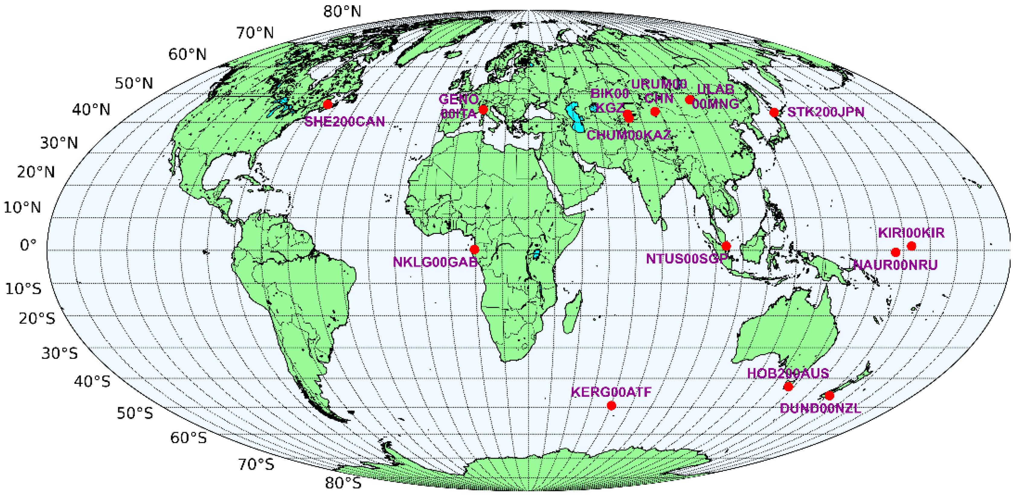
Data from globally distributed GNSS stations were analyzed to determine the potential impact of geomagnetic indices on GPS position accuracy (

Table 1. The initial group of GNSS measurement stations.

GNSS Station	Country	Lat	Lon	Elev	Receiver Type	Antenna Type
BIK00KGZ 1	Kyrgyzstan	42.854	74.533	749.2	Javad TRE_G3TH Delta	JAV_Ringant_ G3T
CHUM00KAZ	Kazakhstan	42.998	74.751	716.3	Trimble NETRS	AOAD/M_T
HOB200AUS	Australia	−42.804	147.438	41.0	Sept PolarX5	AOAD/M_T
DUND00NZL	New Zealand	−45.883	170.597	386.9	Trimble NETR 9	TRM 57971.00
KERG00ATF	French Southern Territories (the)	−49.351	70.255	73.0	Trimble NETR 9	ASH701945E_ M SNOW
KIRI00KIR	Kiribati	1.354	172.922	36.2	Trimble NETR 9	TRM 59800.00
NAUR00NRU	Yaren District, Nauru	−0.551	166.925	46.3	Sept PolarX 4 TR	LEIAR 25.R3
NKLG00GAB	Gabon	0.353	9.672	31.4	Trimble NETR 9	TRM 59800.00
NTUS00SGP	Singapore	1.345	103.679	79.0	Leica GRX 1200 G GPRO	LEIAT 504GG
SHE200CAN	Canada	46.220	−64.552	−15.3	Trimble NETR 8	TRM 29659.00
STK200JPN	Japan	43.528	141.844	118.5	Trimble NETR 9	TRM 59800.00
ULAB00MNG	Mongolia	47.865	107.052	1575.7	Javad TRE_G3TH Delta	JAV_Ringant_ G3T
URUM00CHN	People Republic of China	43.807	87.6	858.9	TPS NETG3	TPSCR3_GGD
GENO00ITA	Italy	44.419	8.921	155.5	Trimble 4700	TRM 29659.00

¹ A loss of lock was recorded during the period from 8 September 02:40 h to 9 September 01:59 h; therefore, data from this station were excluded from further processing.

and Figure 1).

Considering the expected magnetic deviation and the distribution of the Dst index as a response to geomagnetic storms, stations located in the equatorial zone and areas at 45°S and 45°N were selected. The ability of the employed GNSS receivers to track and maintain accuracy during geomagnetic disturbances was not investigated in this study, as it falls outside the scope of the research.

Hourly values of the Dst index produced by Kyoto University, which vary (considering the observed period) from 20 nT to −20 nT during quiet periods and reach −148 nT during geomagnetic storms, were used in this research [47] and are shown in Figure 2.

Since the study is based on positional records from September 2017, the selection was limited to GPS and GLONASS (Global Navigation Observation National Satellite System) satellite navigation systems (other GNSS systems were not operational during that period). Preliminary tests were conducted on positional records from both systems, assessing the initial total position error, which was then used for further statistical analysis to select the optimal GNSS system based on the research premises. The preliminary results indicate that GPS is the optimal GNSS system, with positional results showing a specific response to changes in the Kp index, suggesting a potential (however not yet thoroughly investigated in this initial stage) influence of geomagnetic storms on the positional accuracy movement of the GPS. Characteristic differences between GPS and GLONASS positional accuracy for the same location and period with respect to the Kp index are shown in the Appendix A (OFF delta X, Y, and Z represent positioning error for the corresponding axes of the ECEF (Earth Centered, Earth Fixed) coordinate system; ns represents the number of visible satellites). GLONASS generally exhibits poorer accuracy with significantly larger extreme values of positional error, but does not show a negative response (in terms of pronounced degradation of overall positional accuracy) to the increase in the Kp index during the period of a strong geomagnetic storm. Conversely, GPS (right Appendix A figures) demonstrates noticeably smaller extreme values and more accurate overall positioning, although it also shows a visibly reduced positional accuracy during periods of elevated Kp index. Since the same relationship between satellite systems is observed across all selected measurement locations, further research focuses on the GPS. The observed resilience of the GLONASS system under conditions of intense geomagnetic storms can be interpreted as a consequence of several interacting factors: FDMA signal processing, a larger inherent ephemeris and clock errors, as well as poorer satellite geometry.

The FDMA approach involves creating multiple channels within the existing frequency range of the signal, which contributes to the robustness and resilience of the signal under increased ionospheric turbulence [48], with such signal processing in the receiver exhibiting characteristics similar to dual iono-free combinations. During an intensive geomagnetic storm, ionospheric effects induce TEC fluctuations leading to phase scintillation and code measurement errors [49]. Under geomagnetic disturbance conditions, FDMA frequency diversity provides more stable signal processing because scintillation affects different frequencies independently.

CDMA (Code Division Multiple Access) techniques, applied in GPS systems, utilize the entire radio signal frequency range with codes to separate signals sharing the same frequency band [50]. GPS CDMA signals (all transmitted on the same L1 frequency) tend to correlate ionospheric delays more strongly, amplifying positioning errors during disturbances. Thus, uncorrelated FDMA error distribution across frequencies contributes to GLONASS superior resilience in geomagnetically intensive periods.

Without the application of dual-frequency iono-free combination, in conditions of significantly disturbed dispersive media, CDMA techniques show lower resilience to ionospheric irregularities, leading to degradation in GPS positional accuracy.

Studies confirm that GPS broadcast ephemerides are more precise than those in GLONASS [51]. In quiet conditions, GPS performance generally surpasses that of GLONASS. The same relationship applies to satellite visibility, where poorer GLONASS geometry results in higher noise levels, thereby reducing overall accuracy during quiet periods compared to GPS.

Since ionospheric effects constitute the most significant individual source of positioning error budget, during intense geomagnetic storms, the magnitude of ionospheric errors surpasses other sources within the total positioning error. Consequently, there is a dilution of ionospheric-induced variations within GLONASS’s overall accuracy during such disturbances, whereas the ionospheric impact on GPS is more pronounced and evident.

The September 2017 geomagnetic storm (Kp = 8, Dst = −142 nT) was selected as a representative moderate-intensity event to address this study’s primary objective: to statistically evaluate whether fluctuations in geomagnetic indices (Kp/Dst) exert a measurable and predictable influence on single-frequency GPS positioning accuracy without direct ionospheric modeling. This event fundamentally differs from historically prominent disturbances like the St. Patrick’s Day (2015; Kp = 8, Dst = −223 nT) and Halloween (2003; Kp = 9, Dst = −383 nT) storms in both magnitude and drivers. Key distinctions include its double CME solar trigger (versus 2015’s CME-CIR (Co-rotating Interaction Region) hybrid and 2003’s consecutive CMEs), evolutionary trajectory, and limited auroral expansion. These characteristics position September 2017 as methodologically optimal: its moderate severity avoids the nonlinear complexities of extreme events while providing sufficient perturbation energy to detect GNSS error signatures. Critically, comprehensive GNSS data availability from global networks at high temporal resolution, combined with its self-contained timeline (4–11 September), enables a robust phase-dependent regression analysis of index–error relationships across geographic regions. This controlled framework minimizes confounding variables—a prerequisite for testing the operational hypothesis that geomagnetic indices alone can quantify GPS position degradation under heightened disturbance.

The study used GPS positional records from multiple sources [52] in versions 2 and 3 of the RINEX (Receiver INdependent EXchange) format. Positional accuracy was determined by processing navigation and observation files in RTKLIB software version 2.4.3 b33 [53], expressed in the ECEF geocentric coordinate system. The total GPS position error was calculated as the sum of deviations from the accurate geodetic position along the three axes (in the horizontal and vertical planes). Other initial settings for determining total GPS position error are shown in

Table 2. The initial settings of the RTKLIB program.

Positioning mode	Single
Elevation mask	15°
Ionosphere correction	Broadcast
Troposphere correction	Saastamoinen
Satellite ephemeris/clock	Broadcast
Format	ECEF (x, y, z)

.

2.2. Theoretical Background for One-Way RM ANOVA

Repeated Measures ANalysis Of VAriance (RM ANOVA) or within-subjects ANOVA is a statistical technique used to determine the presence of statistically significant differences between the arithmetic means of logically connected and dependent groups of data. It is applied in situations where the same set of objects is observed at different time intervals or after the influence of external variables (at different time points).

We assume that from an infinite population, n subjects have been randomly chosen and were measured in a dependent and normally distributed variable X through k different time points (or under k different conditions). Furthermore, the $x_{l,m}$ result of the lth subject during the mth measurement is noted. Consequently, the obtained data can be presented as follows:

$$\begin{array}{c}\mathrm{1nd}\mathrm{measurement:}{x}_{\mathrm{1,1}},x_{\mathrm{2,1}},\cdots ,x_{n,1}\\ \mathrm{2nd}\mathrm{measurement:}{x}_{\mathrm{1,2}},x_{\mathrm{2,2}},\cdots ,x_{n,2}\\ ⋮\\ k\mathrm{th}\mathrm{measurement:}{x}_{1,k},x_{2,k},\cdots ,x_{n,k}\end{array}$$

Measurements are presented as columns in data matrices, and there are $n\cdot k$ data in total.

Research hypotheses for One-Way RM ANOVA are as follows:

$$H_0:{\mu }_1={\mu }_2=\cdots ={\mu }_k$$

(1)

$$H_1:{\mu }_i\ne {\mu }_j forsomei,j$$

(2)

Hypothesis (H₀) points to the situation where there is no statistically significant difference amongst the means of measurement over time. Consequently, if H₀ is rejected, one should suppose that differences in measurements during time exist, at least between the ith and jth time point, for some i, j = 1, …, k.

Like in most parametric statistical methods, the mathematical background behind RM ANOVA is an analysis of data variability decomposition [54]. Total variability in such a design is the sum of between-time or between-conditions or “effect” (SSB or SSTime) and within-subject variability (SSW), which can be decomposed as a sum of intrasubject variability (SS_Sub) and error variability (SS_Err).

The term “effect” is used due to the fact that the identification and explanation of differences between measurements over time is the main research problem. Accordingly, the term “error” does not imply mistake; it indicates, from a statistical point of view, the possibility that variance can occur by chance alone, or the variance that is unaccounted for by the effects of subject differences over time.

Finally, the decomposition of variability is obtained:

$$S{S}_T=S{S}_B+S{S}_{Sub}+S{S}_{Err}$$

(3)

From the calculation point of view, total mean (${\overline{x}}_T$), means of measurements in time points ${\overline{x}}_j^t, j=1,\dots ,k$, and means of each subject’s measurements during time ${\overline{x}}_i^s, i=1,\dots ,n$ have to be calculated:

$${\overline{x}}_T={\displaystyle \frac{{\sum }_{j=1}^k{\sum }_{i=1}^n{x}_{i,j}}{n\cdot k}}; {\overline{x}}_j^t={\displaystyle \frac{{\sum }_{i=1}^n{x}_{i,j}}{n}}; {\overline{x}}_i^s={\displaystyle \frac{{\sum }_{j=1}^k{x}_{i,j}}{k}}$$

(4)

The sums of squares—total (SS_T), between-time (SS_B), subjects (SS_Sub), and error (SS_Err)—are calculated:

$$S{S}_T={\sum }_{j=1}^k{\sum }_{i=1}^n(x_T-x_{i,j}{)}^2$$

(5)

$$S{S}_B=S{S}_{Time}={\sum }_{j=1}^k{\sum }_{i=1}^n(x_T-{\overline{x}}_j^t{)}^2={\sum }_{j=1}^{k}n(x_T-{\overline{x}}_j^t{)}^2=n{\sum }_{j=1}^k(x_T-{\overline{x}}_j^t{)}^2$$

(6)

$$S{S}_W={\sum }_{j=1}^k{\sum }_{i=1}^n({\overline{x}}_j^t-x_{i,j}{)}^2$$

(7)

$$S{S}_{Sub}={\sum }_{j=1}^k{\sum }_{i=1}^n(x_T-{\overline{x}}_i^s{)}^2={\sum }_{i=1}^{n}k(x_T-{\overline{x}}_i^s{)}^2=k{\sum }_{i=1}^n(x_T-{\overline{x}}_i^s{)}^2$$

(8)

Considering that mean squares (MS) are computed if each sum of squares is divided by the appropriate degrees of freedom, the following is obtained:

$$M{S}_T={\displaystyle \frac{S{S}_T}{d{f}_T}}={\displaystyle \frac{S{S}_T}{nk-1}}$$

(9)

$$M{S}_B={\displaystyle \frac{S{S}_B}{d{f}_B}}={\displaystyle \frac{S{S}_B}{k-1}}$$

(10)

$$M{S}_{Sub}={\displaystyle \frac{S{S}_{Sub}}{d{f}_{Sub}}}={\displaystyle \frac{S{S}_{Sub}}{n-1}}$$

(11)

$$M{S}_{Err}={\displaystyle \frac{S{S}_{Err}}{d{f}_{Err}}}={\displaystyle \frac{S{S}_{Err}}{(k-1)(n-1)}}$$

(12)

and finally, the F-value can be calculated

$$F\left(d{f}_B,d{f}_{Err}\right)={\displaystyle \frac{M{S}_B}{M{S}_{Err}}}$$

(13)

Data are usually reported in a so-called ANOVA table, as presented in

Table 3. RM ANOVA.

Source of Variation	SS	df	MS	F	P
Between time points/conditions (effect)	SSB	k − 1	MSB	F	P
Error	SSErr	(k − 1)(n − 1)	MSErr
Within subjects	SSSub	n − 1
Total	SST	nk − 1

.

The independence of df_B and df_Err together with the Type I error (α, usually set at 5%) critical F-value is calculated. Equivalently, empirical significance p is calculated, and if p < α, hypothesis H₀ is rejected. The fundamental difference in calculation logic between within-subjects ANOVA and between-subjects ANOVA is that the within-subject variability from repeated measures is adjusted for variability from subject to subject to obtain error variability, SS_Err. More simply, SS_Err is adjusted for the within-subjects dependency of the measures. In order to assess the potential influence of the observed parameters Kp and Dst indices on the total GPS position error and to expand the understanding of their mutual relationships, a statistical variance analysis of the data was conducted on the selected dataset. Additionally, independent and dependent variables were subjected to regression analysis.

3. Results

Variance (or a measure of data dispersion) determines the absolute variability of data within each dataset. In the conducted research, the period of Earth’s response to geomagnetic storms (depending on the location of the measurement station) spans from the end of 6–9 September, and accordingly, data series were formed and subjected to statistical analysis. By interpolating the Kp index (3 h data frequency) and the Dst index (1 h data frequency) and aligning them temporally (by UTC), data for the entire month of September 2017 were prepared for all observed locations. Thus, each data series contains temporally aligned data on GPS position accuracy (mean value of the total position error) and the corresponding Kp and Dst indices at each time point. Through variance analysis, we aim to identify the level and significance of variability for the input parameters Kp index, Dst index, and the parameter of total GPS position error movement.

To meet the condition that each input dataset must have the same length of temporal data distribution, the input data encompasses three identical time periods: immediately before the geomagnetic disturbance, during the geomagnetic disturbance, and immediately after its end. The data are grouped in 2.5-day successions (period before the geomagnetic storm, during the storm, after the storm, and the entire month of September 2017), as shown in Figure 3.

Furthermore, the input data are grouped by locations: locations within the 45°N zone, the equatorial zone, and the 45°S zone.

RM ANOVA involves setting up two hypotheses: the null hypothesis (${\mathrm{H}}_0$), which states that there is no difference in the arithmetic means of the observed data groups, and the alternative hypothesis (${\mathrm{H}}_1$), which states that there is a difference in the arithmetic means of at least one group of data.

The hypotheses in the variance analysis are as follows:

$$H_0={\overline{X}}_1={\overline{X}}_2=\cdots ={\overline{X}}_n$$

(14)

where ${\overline{\mathrm{X}}}_{\mathrm{i}}$ i = 1, … n are the arithmetic means of the i-th measurement (each individual input data group).

The null hypothesis ${,\mathrm{H}}_0$, which we accept if p > 0.05, indicates no significant difference between the means, meaning the effect of the independent variables (Kp and Dst indices) on GPS position accuracy is not identified.

Conversely, the alternative hypothesis ${\mathrm{H}}_1$ states the following: there exist i, j such that $H_i\ne H_j$, i.e., a difference between the arithmetic means is established. Therefore, we consider the observed effect of the random variables (Kp and Dst indices) on total GPS position error to be statistically significant. Considering the large input dataset, and employing the Central Limit Theorem from mathematical statistics, we conclude that the data exhibit a tendency towards a normal distribution. Furthermore, the homogeneity of variances was assessed using Levene’s test, which indicated that there is no violation of variance homogeneity among the separate blocks of the input data (p > 0.05).

In the statistical analysis, variance analysis examines the ratios of variability to determine whether the F-value exceeds the critical F-value. The analysis calculates the F-statistic (test statistic value) and the p coefficient (level of statistical significance). The identification of statistical significance can be interpreted as the effect of geomagnetic storms expressed through Kp and Dst index values on the total GPS position error. The obtained statistical results of the variance analysis for the observed variables are presented in

Table 4. Variance test results.

Area	Period September 2017	Total GPS Position Error			Kp Index			Dst Index
		Var	F	p	Var	F	p	Var	F	p
45°N	4–6	10.41	0.75	>0.05	0.82	0.33	>0.05	35.63	0.02	>0.05
	7–9	15.22	1.73	<0.001	3.51	3.34	<0.001	2588.14	61.89	<0.001
	10–11	4.72	0.36	>0.05	1.62	0.62	>0.05	57.11	0.04	>0.05
0°	4–6	18.58	0.89	<0.001	0.82	0.31	>0.05	35.63	0.02	>0.05
	7–9	23.68	1.35	<0.001	3.51	3.22	<0.001	2588.51	63.08	<0.001
	10–11	15.14	0.88	<0.001	1.51	1.63	>0.05	51.96	0.03	>0.05
45°S	4–6	4.20	0.58	>0.05	0.82	0.34	>0.05	35.45	0.02	>0.05
	7–9	10.57	2.82	<0.001	3.54	3.21	<0.001	2592.41	62.34	<0.001
	10–11	2.85	0.41	>0.05	1.64	0.63	>0.05	53.66	0.03	>0.05

.

The results indicate statistically significant latitudinal and temporal variations in total GPS position error during the September 2017 geomagnetic storm. The variance of total GPS position error demonstrates distinct patterns across the three examined periods, ranging from 2.85 (10–11 September, 45°S) to 23.68 (7–9 September, Equator). The F-statistics show particularly strong evidence of disturbance during the main storm phase at all latitudes, with values of 1.73 (45°N), 1.35 (Equator), and 2.82 (45°S), all with p < 0.001. This demonstrates that the internal dispersion of total GPS position error data statistically differs depending on the selected time period and geographic area, and that this dispersion difference is statistically significant. Notably, the equatorial region exhibits the highest absolute error variance (23.68) during storm conditions, while the southern hemisphere maintains the most stable measurements, as evidenced by the lowest variance values across all phases. The p-values < 0.001 for the storm period at all latitudes allow us to reject the null hypothesis of uniform error distribution, thereby supporting the hypothesis of external influences and the unpredictability of total GPS position error movement within parts of the observed period.

In the context of this research, one of the external factors that potentially influences total GPS position error is the global geomagnetic activity in the Earth’s magnetosphere, expressed through the Kp index value. The analysis of Kp index variability shows consistent storm phase patterns across latitudes. During quiet conditions (4–6 September), all areas exhibit low variance (0.82) with statistically insignificant F-values (0.31–0.34, p > 0.05). The storm phase (7–9 September) demonstrates significant increases in variance (3.51–3.54) and F-statistics (3.21–3.34, all p < 0.001), with the most pronounced effects at 45°N (F = 3.34). This latitudinal pattern persists into the recovery phase (10–11 September), where variance decreases to 1.51–1.64, accompanied by non-significant F-values (0.62–0.63, p > 0.05). The consistent p-values < 0.001 during the storm period confirm that Kp index variability is not uniform across time periods and is influenced by external geomagnetic disturbances.

Another potential external factor which might exert a statistically significant influence on the movement of total GPS position error is the Dst index, which indirectly reflects the effects of geomagnetic storms on technical systems, primarily radio communication satellite systems [8]. Its influence on variations in the magnetic field is mainly attributed to geomagnetic storms and solar wind, where increased intensity results in the release of charged particles that become trapped in Earth’s magnetic field, forming a ring current. Since Dst is usually analyzed alongside other space weather indices, particularly the Kp index, it was included in this study. The Dst index analysis reveals extreme variations during the storm period, with variance values reaching 2588.14–2592.41 across all stations (7–9 September). The corresponding F-statistics are exceptionally high (61.89 at 45°N, 63.08 at Equator, 62.34 at 45°S), all with p < 0.001, indicating a dramatic intensification of ring current activity. During quiet conditions (4–6 September), Dst variance remains low (35.45–35.63) with insignificant F-values (0.02, p > 0.05). The recovery phase shows partial normalization, with variance decreasing to 51.96–57.11, though still maintaining elevated levels compared to pre-storm conditions. Considering the p-values < 0.05, we conclude that the internal dispersion of Dst index fluctuations variations is statistically significant and depend on external influences, which are identified as geomagnetic storms and solar disturbances.

Beyond the statistical parameters described for the three temporally and spatially defined input variables, an analysis of variance was also performed on a dataset covering the entire September 2017 period. The daily dynamics of variance for Kp, Dst, and total GPS position error are presented in Figure 4, Figure 5 and Figure 6.

An analysis of Figure 3, Figure 4 and Figure 5 reveals several common trends: during the geomagnetic storm from 7 to 9 September, there is a noticeable “synchronization” in the behavior of the movement of variances of the Kp index and the total GPS position error across all observed latitudes. It appears that an increase in the variability of the Kp index occurs first (towards the end of 6 September), which is followed, with a time delay of approximately one day, by an increase in the variability of the total GPS position error. The same trend is observed during 8–9 September as the geomagnetic storm subsides, when the variability of the Kp index decreases (the global Kp index values return to pre-disturbance levels with Kp ≤ 5, which at that time has no significant impact on Earth’s magnetic field). The reduction in variance of the Kp index during this period, with a one-day delay, is accompanied by a decrease in the variability of the total GPS position error. Identical behavior is observed during 27–28 September, during which an increase in the variability of the total GPS position error is also recorded. Unlike the first observed period, when the variances of the total GPS position error reach their maximum within the same timeframe (9 September) across all observed latitudes, in the second period (27–28 September), the maximum variance of the total GPS position error occurs in the area of 45°N and the Equator one day earlier than in the area of 45°S.

A similar pattern is observed in the relationship between the movement of the variances of the Dst index and the total GPS position error during the observed period and throughout September 2017. The tendency of “synchronization” the total GPS position error variance in relation to the Dst variance for the period 7–9 September is evident, along with its spatial unevenness. During the second period of heightened geomagnetic activity (27–28 September), a sharp increase in the variances of both parameters is detected, with the Dst variance showing a significantly greater degree of dispersion than during 7–9 September, when geomagnetic activity was at its peak.

The differences observed in the measurements are indirectly attributed to the intensity of the geomagnetic storm (Kp index) and directly to the Dst index as a measure of the strength of the magnetosphere during geomagnetic storms. Although it has been demonstrated that the quality of radio propagation in certain wave bands (primarily LF/MF) [8] can be satisfactorily predicted based on the Dst index, the complexity of the internal dynamics of the current ring prevents definitive conclusions.

4. Discussion

Although we can generally conclude that geomagnetic storms lead to decreased GPS positional accuracy, it is necessary to avoid spurious correlation claims and conduct further statistical analysis. To determine the degree, direction, and intensity of the relationship between the observed geomagnetic indices and the total GPS position error, a regression analysis was performed on the set of these parameters. The regression analysis was conducted separately for each period (before, during, and after the geomagnetic storm) and for the entirety of September 2017.

The presented results of the regression analysis include several parameters: the R² parameter explains what proportion of the dependent variable (total GPS position error) can be explained by the effect of the independent variables (Kp and Dst indices). A higher value indicates a greater level of influence, while the F-statistic test evaluates the overall significance of the regression model. The F-parameter indicates how the regression model with included predictors describes the data more precisely compared to a model without predictors, with a higher F-value suggesting an improved model fit. The p parameter shows the statistical significance of the relationship between the observed predictor (Kp and Dst individually) and the dependent variable. The conventional threshold p-value is set at 0.05; a smaller value indicates that the relationship between the dependent and independent variables is statistically significant. A larger value suggests that the hypothesis of their association can be rejected, implying that the predictor has no statistically significant impact on the dependent variable. The values in the “Kp index impact” column indicate the intensity with which a one-unit change in the independent Kp variable affects the movement of the accuracy (in absolute value [m]) of the dependent variable (total GPS position error).

The results of the regression analysis for the Kp index are shown in

Table 5. Regression analysis results for the Kp index.

Period	Area	R2	F	p	Kp Index Impact
4–6 September	45°N	0.0001	0.368	0.543	−0.04
	0°	0.009673	21.077	<0.001	0.470
	45°S	0.001195	2.555	0.110	−0.079
7–9 September	45°N	0.004	14.439	<0.001	0.116
	0°	0.000085	0.183	0.668	−0.019
	45°S	0.006154	13.227	<0.001	0.103
	45°N	0.00003	0.082	0.773	0.013
10–11 September	0°	0.012150	22.693	<0.001	−0.347
	45°S	0.000087	0.187	0.664	0.016
	45°N	0.004	131.2	<0.001	0.129
September 2017	0°	0.011	273	<0.001	0.275
	45°S	0.002	44.677	<0.001	0.057

(for the observed periods and the entire September 2017), as well as graphically in Figure 7 (September 2017).

The influence of the Kp index on total GPS position error varies by period and region. At 45°N, its effect depends on the period: no significant influence was observed immediately before an intense geomagnetic storm. During the storm (7–9 September), the effect was statistically significant (F = 14.4); however, it only accounted for 0.4% of the GPS error. No significant effect was found during the recovery phase.

For equatorial stations, the Kp index significantly influenced GPS error before and after the storm, improving model definition (F = 21, F = 22.6). However, during the intense storm peak, despite high Kp values, no significant effect was observed (p-value = 0.6).

The dynamics at 45°S mirrored 45°N: significance only during the main storm phase (F = 13.2, accounting for 0.6% of error), with no effect before or after. Analyzing 4–11 September reveals a pattern: during the quiet (initial) and recovery (final) periods, the Equator shows significant susceptibility to global magnetospheric dynamics. Conversely, mid-latitudes (45°N/S) show no significant susceptibility to intense geomagnetic influence causing abnormal error oscillations during these times. During the intense storm, mid-latitudes show influence, while the Equator shows none (based on used stations). Across all areas during September 2017 (including two periods of Kp > 5), a significant Kp effect is observed. The regression model showed the highest improvement including Kp for the Equator (F = 273), accounting for the largest error portion (1.1%).

The analysis is supplemented by Kp impact values. Statistically negative intensities (indicating improved GPS accuracy with increasing Kp) were observed for 45°N/S during 4–6 September and for the Equator during 7–11 September. This relationship was not significant in three cases but was significant for the Equator on 10–11 September, yielding the greatest absolute improvement (0.34 m per Kp unit) and accounting for the largest error part (1.2%). Considering the entire month, a significant positive Kp impact (accuracy degrades with increasing Kp) was observed, with absolute values from 5.7 to 27.5 cm. The proportion of GPS error attributable to Kp ranged from 0.2% (45°S) to 1.1% (Equator). Analyzing error distribution shows a fairly uniform spread in September 2017, with maximum deviations occurring when Kp ≤ 5 (low activity).

The Dst index describes the ring current state [8], with negative values indicating disturbances. For all areas, the greatest GPS error occurred at minimum Dst values (lowest: −148 nT). No clear pattern was observed for Dst > −100 nT. Generally, oscillation trends were evident up to Dst = −100 nT, followed by clear degradation as Dst decreased further. The results are in

Table 6. Regression analysis results for the Dst index.

Period	Area	R2	F	p	Dst Index Impact
4–6 September	45°N	0.004030	11.644	<0.001	0.0365
	0°	0.000798	1.724	0.190	−0.0224
	45°S	0.01475	32	<0.001	0.0469
7–9 September	45°N	0.014	39.68	<0.001	0.0095
	0°	0.037	82.787	<0.001	−0.0199
	45°S	0.003056	6.548	0.01	−0.0036
10–11 September	45°N	0.003645	9.348	0.002	0.0134
	0°	0.005191	9.627	0.001	−0.0240
	45°S	0.002779	6.006	0.014	0.0091
September 2017	45°N	0.000027	0.899	0.343	0.0007
	0°	0.015721	386.773	<0.001	−0.0218
	45°S	0.002	37.641	<0.001	−0.0035

and Figure 7.

Regression shows the Dst effect to be more uniform. When looking at the period from 4 to 11 September, Dst had no significant effect on the Equator from 4 to 6. In other periods across all regions, it significantly impacted GPS error, with the highest F-statistic during the storm at the Equator (F = 82), accounting for 3.7% of error. Monthly, Dst maintained significance for the Equator (F = 386) and at the 45°S latitude. Despite the high F-value, the highest monthly explained error was 1.5% (Equator). Dst did not statistically influence GPS error at the 45°N latitude each month.

Ring current strengthening (weakening surface magnetic field) does not uniformly impact GPS. While Dst exerted a significant impact in eight of the nine observed cases, the coefficients showed both positive and negative interactions. Besides presumed degradation, a statistically significant improvement in GPS error was also observed during analyzed periods and throughout September 2017 (Equator). Degradation per Dst unit change over the entire month was not significant, while an absolute statistically significant accuracy improvement (0.35 cm to 2.18 cm) was achieved.

5. Conclusions

The conducted research and applied statistical methods (variance analysis) demonstrated that the dispersion of the total GPS positioning error is not random and can be statistically attributed to the influence of geomagnetic storms, expressed through the Kp index and ring current dynamics. The dynamics of single-frequency GPS position movement during periods of intense geomagnetic disturbance deviate from their behavior in comparison to identical periods before and after the event. However, regression analysis provides a more comprehensive picture of the interrelationships: depending on the geographical area and storm phase, the influences of the Kp and Dst indices exhibit significant spatial and temporal variations. For the Kp index, statistically significant effects were confined primarily to the main storm phase (7–9 September) at mid-latitudes (45°N: F = 14.4; 45°S: F = 13.2), accounting for only 0.4–0.6% of error variance. Conversely, equatorial regions showed significant Kp influence during quiet and recovery phases (F = 21–22.6) but not during peak disturbance. The Dst index demonstrated more uniform significance across phases and regions, with the strongest effect during the storm at the Equator (F = 82, explaining 3.7% of error) and maintaining monthly significance at the Equator (F = 386) and 45°S. Paradoxically, both indices showed instances of significant negative impacts, where intensifying geomagnetic activity improved positioning accuracy—most notably for Kp at the Equator during recovery (0.34 m improvement per unit increase, explaining 1.2% of error) and for Dst across equatorial regions (0.35–2.18 cm monthly improvement). In periods and locations where the Kp and Dst indices achieve statistical significance, they explain only a minimal portion of GPS error variance (≤3.7% for Dst during storms, ≤1.5% monthly). Moreover, their most significant impacts actually reduced total GPS error in specific instances.

The regression results demonstrate that the observed geomagnetic indices’ spatial and temporal uneven influence on the dynamics of total GPS positioning error occurs in a way that precludes direct and unequivocal interpretation. This leads to the rejection of the previously formulated hypothesis regarding the possibility of predicting total GPS positioning error position solely based on selected geomagnetic indices. This study represents an attempt to determine potential correlations between Dst/Kp indices and total GPS positioning error during intensive geomagnetic events without presuming known relationships. While confirming non-random variability during the storm period (7–9 September) attributable to geomagnetic disturbances, the results do not support definitive correlation between these indices and total GPS positioning error. The stochastic nature of geomagnetic storms resists full statistical description through these indices alone, though identifiable behavioral patterns emerged.

The research results show that the Kp and Dst indices, which describe the intensity of geomagnetic storms and disruptive ring current as input independent variables, and the total GPS error as the dependent variable, cannot be directly correlated for predictive purposes. Nevertheless, the fact of the measurable observed similarity between the variance trends of positioning errors and those of geomagnetic indices reveal the need for further investigation. This indicates that the ionosphere is an indispensable factor, both in error generation and in the prediction of satellite-determined position errors caused by space weather disturbances. However, the developed methodology provides a foundation and points towards the design of future research on ionosphere response (observed through characteristic parameters, primarily TEC dynamics) to geomagnetic disturbances. On the other hand, numerous previous studies confirm the influence of ionospheric parameters on satellite navigation service errors, and this relationship can also be tested using the adopted methodological approach. In further research, it is necessary to decompose the GPS positioning error vectorially along the x, y, z axes to establish the displacement value dynamics of the GPS positioning error expressed by the geometry of the space along the axes as a function of TEC.