Seasonal and Long-Term Water Regime Trends of Cheremsky Wetland: Analysis Based on Sentinel-2 Spectral Indices and Composite Indicator Development

Abstract

Wetlands are critically important ecosystems, but their dynamics, especially in complex regions such as the Ukrainian Polissya, remain poorly understood. This study focuses on the Cheremsky Nature Reserve, an internationally important wetland, to assess long-term (2017–2024) seasonal (spring-summer) trends in water surface conditions. Using Sentinel-2 data and the Google Earth Engine platform, 14 spectral water indices were calculated. Their temporal trends were analyzed using Sen’s method, mutual correlations, and principal component analysis (PCA) to identify the main patterns of variability. Based on the normalized trends and weights obtained from the first two principal components, an integral composite index (CI) for spring and summer seasons was developed. The results revealed seasonal differences in the behavior of the indices and their contribution to the principal components, as well as spatial differentiation of water regime trends within the reserve. The proposed CI allows for an integrated assessment of the long-term dynamics of the wetlands, which is important for the development of conservation and management strategies.

1. Introduction

The designation “wetland” is a broad term that can be defined in a variety of ways.

Wetlands are defined as areas that are subject to high levels of moisture and are accompanied by the presence of certain species of animals and plants, as well as other organisms. A wetland is defined as an area that is subject to excessive moisture and is accompanied by hydrophilic vegetation and/or organic soils. Wetlands are defined as transient ecosystems situated on the border between typical aquatic and terrestrial systems. They are formed under conditions of permanent or periodic waterlogging of the land surface, resulting in hydrophilic vegetation and the accumulation of organic soils. It is evident that there are numerous definitions of the term [1].

The term “bogs and marshes” is used to refer to wetlands that are distinguished by the accumulation of peat.

Wetlands and bogs are defined as areas of land characterized by a high water table or saturated soil, often with no clearly defined boundaries. The term “marsh” is employed to denote herbaceous vegetation that is characteristic of an undated environment.

The terms “wetlands” and “bogs” are used to refer to “forested wetlands” or other similar geographical features, without the use of standardized nomenclature.

The Ramsar Secretariat [2] asserts that wetlands are defined as areas where water exerts a predominant influence on the environment. The environment and its associated flora and fauna are of particular concern. The occurrence of this phenomenon has been observed in areas where the water table is at or in close proximity to the ground surface. In instances where the land is distinguished by the presence of shallow water, this phenomenon has been observed. In this and other studies, we will use this definition for clarity of further results and conclusions.

The Convention on Wetlands [3] constitutes an international agreement whose stated aim is to protect and preserve wetlands on a global scale.

Remote sensing has become a crucial technology for evaluating wetland health and dynamics, providing spatially explicit, cost-effective, and non-invasive solutions [4,5,6,7]. In this context, multispectral indices derived from satellite imagery have become essential for quantifying vegetation vitality, water availability, and soil moisture—key parameters for understanding wetland ecosystem functioning.

The Sentinel-2 mission [8], with its high spatial (10–20 m) and temporal (5-day revisit) resolution, provides effective opportunities for monitoring fine-scale changes in heterogeneous wetland environments. In combination with cloud-based platforms such as Google Earth Engine (GEE) [9], which enables efficient processing of large-scale geospatial datasets, Sentinel-2 imagery supports the calculation of a wide range of spectral indices commonly used in water dynamics research.

Belloli et al. [10] investigated the potential of multispectral bands and spectral indices from PlanetScope and Sentinel-2A satellites for estimating above-ground biomass (AGB) and organic carbon (Corg) in reed vegetation in wetlands. They found that spectral indices were better correlated and better suited as predictor variables. The most accurate model used PlanetScope data and the photochemical reflectance index (sPRI). Both sensors showed potential for pixel-based AGB and Corg estimates. CO2Flux VI (which includes PRI and NDVI) showed a significant correlation with biophysical variables for Sentinel-2A. Although indices formed from Sentinel-2A red edge bands did not show significant correlations, higher correlations were expected. This may be due to the fact that changes in the position of the red edge band can occur during floods, which may reduce the effectiveness of NDRE indices in remote sensing applications.

This study also compared NDAVI and WAVI with NDVI and SAVI, finding that NDAVI and WAVI exhibited superior discrimination characteristics for wetland vegetation. This finding serves to substantiate the hypothesis that NDAVI can be associated with the biophysical data of vegetation and used to monitor its dynamics.

Ade et al. [11] successfully applied Sentinel-2 multispectral data and machine learning classifiers to map invasive floating aquatic plants at the genus level. Random Forest models with Sentinel-2 data achieved an average overall accuracy of 90%, with class accuracies ranging from 79–91% for water hyacinth and 85–95% for water primrose. They used a wide range of spectral indices, including NDVI, NDAVI, WAVI, SAVI, NDWI, NDMI, MNDWI, as well as red edge indices (NDVIRe2, NDVIRe3). The study showed that spectral indices consistently ranked high in importance in all three models. The SWIR range and indices calculated with it were important for the performance of the Random Forest model and for distinguishing aquatic vegetation from water. The paper observes that spectral indices consistently ranked high in terms of importance in the classification process. However, the “red edge” ranges, despite their contribution, received a lower rating compared to other spectral indexes and spectral ranges in the visible and shortwave infrared spectrums.

The integration of spectral indices with other data sets is a critical step in the analysis. Yu et al. [12] conducted a study that examined the extraction of information regarding wetlands by integrating Sentinel-1/2 images, terrain data, and field observations. The researchers extracted 22 characteristic variables, including spectral bands, spectral indices (especially “red edge” indices), terrain features, and radar features. The incorporation of red edge, terrain, and radar data led to a substantial enhancement in the precision of the extracted land cover information.

Salas et al. [13] employed Sentinel-2 imagery to automate the classification of diminutive wetlands through the implementation of machine learning algorithms. It was determined that NDWI is a significant predictor in the context of wetland mapping. Additionally, it was emphasized that the bands B4 (red), B11 (SWIR), and NDVI are the primary variables for wetland mapping. The presence of other spectral bands, including B8, B5, and B2, has also been demonstrated to be significant in the differentiation of wetlands from other land cover classes.

In a recent study, Usman et al. [14] sought to estimate water levels in wetlands. To this end, the researchers employed integrated multi-source remote sensing data from Sentinel-2 and Landsat-8. The researchers employed the NDWI, two versions of MNDWI, and WRI. The study demonstrated that MNDWI exhibited superior performance in comparison to other water indices for both satellite data sources. The optimal threshold for Sentinel-2 was −0.35, and for Landsat-8, it was −0.25. The SWIR bands incorporated into MNDWI exhibited heightened sensitivity to wetland moisture characteristics, thereby facilitating more precise distinctions between diverse land cover types. This study also indicates that MNDWI generally performed better than NDWI and WRI in distinguishing water surfaces in Sentinel-2 and Landsat-8 images. This phenomenon can be attributed to MNDWI’s capacity to accentuate water signals in diverse terrestrial environments and the sensitivity of SWIR bands to moisture. NDWI and WRI demonstrated reduced accuracy due to their development being predicated on constant clear waters with minimal sediment concentration.

Mahdianpari et al. [15] proposed a Deep Convolutional Neural Network (DCNN) for generating and classifying Sentinel-1 and Sentinel-2 data. To enhance the precision of classification, a range of spectral indices was incorporated, including NDVI, EVI, DVI, RENDVI, and NDWI. The most influential variable for vegetation classification, particularly in the context of wetlands, was found to be the Normalized Difference Vegetation Index (NDVI). This index possesses the capability to minimize noise, thereby facilitating optimal differentiation between wetland and non-wetland classes.

A number of studies have directly compared the performance of different spectral indices for monitoring wetlands, thereby providing significant insights into their effectiveness under various conditions. Solovey [16] investigated the effectiveness of MNDWI, NDPI, and NDTI indices obtained from Sentinel-2 for mapping flooded wetlands. The findings indicated that the amalgamation of these water indicators exhibited superiority in detecting flooding, particularly in wetland areas, when compared to the application of individual spectral water indices. MNDWI is the most effective method for identifying open water, NDPI is the most effective method for capturing vegetation in wetlands and water, and NDTI is the most effective method for reducing the influence of open soil.

In order to enhance the precision of wetland mapping and monitoring, spectral indices are frequently integrated with additional data sources and sophisticated analysis techniques.

SAR (Synthetic Aperture Radar) sensors, such as Sentinel-1, are capable of acquiring images irrespective of cloud cover and weather conditions, rendering them indispensable for wetland monitoring, particularly in regions characterized by substantial cloud cover. The integration of optical and Synthetic Aperture Radar (SAR) data, in conjunction with terrain data, has been shown to enhance the accuracy of wetland classification when compared to the use of optical data alone [17,18].

Topographic indices [12,18], including the Topographic Wetness Index (TWI) and the Topographic Position Index (TPI), play a pivotal role in accurately delineating the location and extent of wetlands. This is due to the fact that terrain exerts a significant influence on the positioning of these ecosystems.

The development of sophisticated machine learning tools, including Random Forest (RF), Support Vector Machine (SVM), and Convolutional Neural Networks (CNNs), has significantly enhanced the capacity for large-scale, reliable, and reproducible mapping and monitoring of wetlands [13,18]. These algorithms have been demonstrated to efficiently process voluminous data sets obtained from satellites to accurately classify wetland land cover types.

Despite their widespread application, the interrelationships and complementarities among spectral indices in wetland environments remain insufficiently investigated. Prior research [16,19,20] has demonstrated that wetlands across different geographic regions require tailored approaches in selecting the most effective combinations of indices for accurate monitoring and analysis. Notably, the Cheremskyi Nature Reserve—a Ramsar-designated wetland of international importance in Ukraine, characterized by a complex mosaic of marshes, peatlands, and floodplain forests—has not yet been systematically assessed using advanced remote sensing techniques. Remote sensing technologies using widely available medium-resolution optical data [21,22,23,24] will complement existing studies of the geological environment, geophysical fields, geomorphosphere [25], hydro- and atmosphere, soil and vegetation cover, and fauna [26], while the analysis of specialized spectral indices will allow for the assessment of processes in vegetation, water, and soil cover. Notwithstanding the ecological significance of Cheremskyi Nature Reserve, no studies have yet employed multi-temporal spectral indices analysis to characterize its hydrological dynamics.

This is a significant gap in understanding long-term changes in wetlands in this region, so one of the objectives of this study will be to assess the spatial and temporal (seasonal and long-term) patterns of changes in the state of water surfaces in the Cheremsky Nature Reserve using a set of 14 spectral water indices calculated based on Sentinel-2 data for the period 2017–2024. The selected time period corresponds to the time of active use of Sentinel-2 satellites and, accordingly, a sufficient number of available images.

A comprehensive review of the extant literature and consultation with leading experts in the academic community have identified a set of key spectral indices for use in the research project. The selection of these indices was made on the basis of their widespread use and relevance to the study. Their employment in the research will ensure its rigor and validity. The relationships (correlations) between different water spectral indices and their seasonal dynamics will be investigated to identify the most informative and complementary indicators of the wetland’s state. These include the Automated Water Extraction Index (AWEI), Difference between Vegetation and Water (DVW), Index of Free Water (IFW), Modified Index of Free Water (MIFW), Modified Normalized Difference Water Index (MNDWI), Water Impoundment Index (WII), Water Ratio Index (WRI), Water Turbidity Index (WTI), and the Augmented Normalized Difference Water Index (ANDWI). Additionally, indices specifically designed for wetland environments—such as the Water in Wetlands (WIW) index—are employed, alongside recently developed water-focused indices tailored to Sentinel-2 data, including the Sentinel Multi-Band Water Index (SMBWI) and the Sentinel-2 Water Index (S2WI).

Each of the mentioned indices will be further discussed and analyzed in detail in the next section.

The present study has two additional objectives. Firstly, it seeks to identify the primary factors of variability in the state of water surfaces using principal component analysis (PCA). Secondly, it aims to assess seasonal differences in the structure of these factors.

The primary objective of this study is to develop and test a methodology for calculating an integral composite index of long-term trends of water surfaces based on PCA for a comprehensive assessment of the dynamics of the Cheremsky Nature Reserve.

This research gap hinders the development of conservation and management strategies based on data ranging from micro to macro levels for such ecologically vulnerable and dynamic landscapes.

2. Materials and Methods

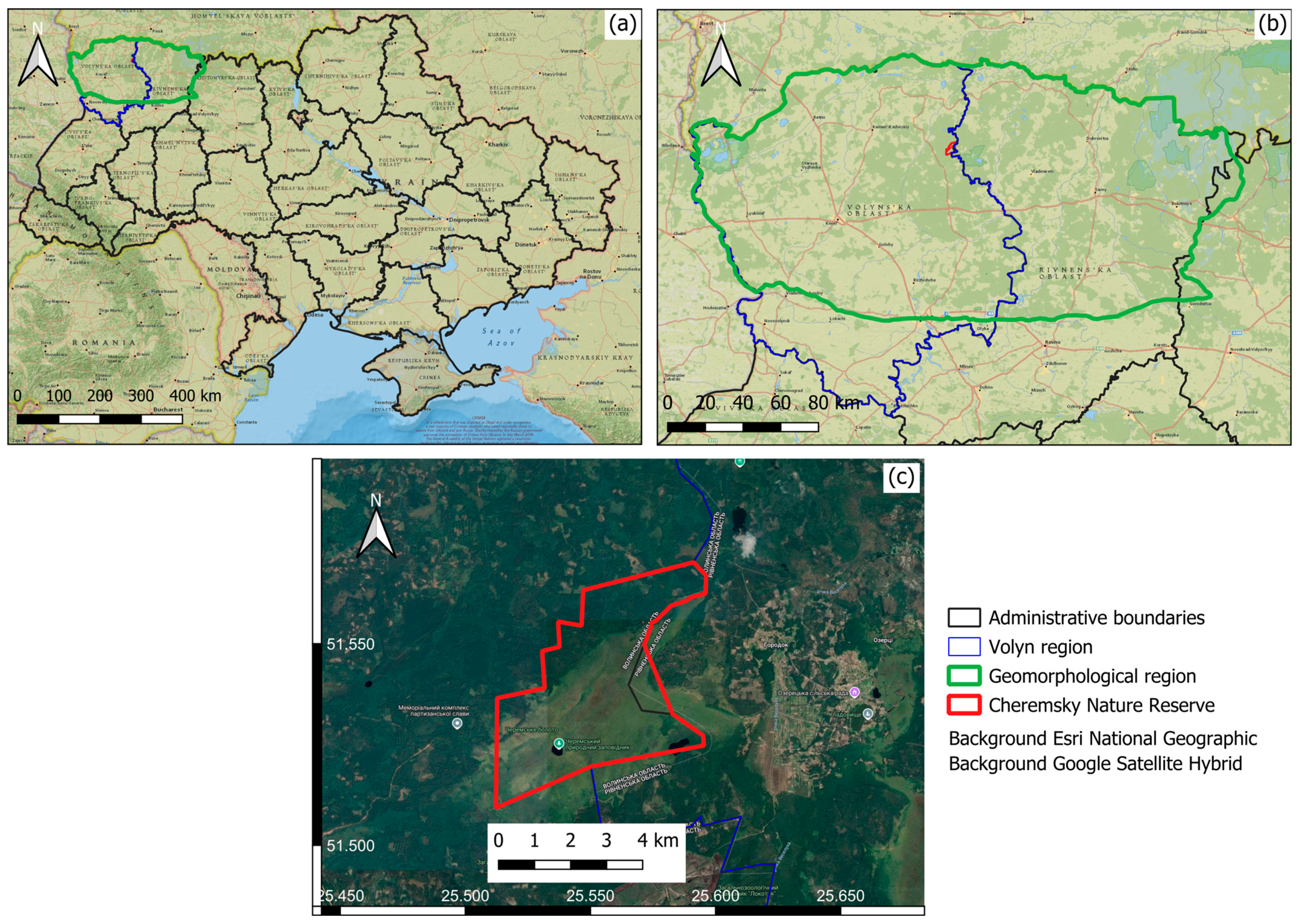
2.1. Study Region

The Cheremsky Nature Reserve, a distinctive ecological preserve, holds a unique status as the sole nature reserve in the Volyn region and is among the northernmost reserves in Ukraine. The establishment of the reserve was formally declared through Presidential Decree No. 1234 of 19 December 2001, which was issued on the basis of the Cheremsky Reserve of national importance, encompassing an area of 903 hectares, in conjunction with its designated protection zone. The reserve also encompasses three reserves of local importance: the ornithological reserve “Suzanka tract,” the general zoological reserve “Karasynsky,” and the botanical reserve “Karasynsky spruce-1.” The total area of the reserve is 2975.7 hectares, of which 64.5% is covered by forests and 33.7% by marshes.

The Cheremsky Nature Reserve is geographically located in the northeastern portion of the Volyn region, specifically in the Manevychi district. Its precise geographical coordinates are between 51°51′ and 51°58′N latitude and between 25°51′ and 25°60′E longitude. This location is within the administrative district of Western Polissya and the Kamin–Kashyrskyi area of the Volyn region. The reserve is situated on the border that intersects with the Rivne region, approximately 6 km north of the village of Zamostia (Figure 1).

The Cheremsky Nature Reserve was established with the primary goal of conserving the unique and irreplaceable natural ecosystems of Western Polissya, which hold exceptional ecological, aesthetic, educational, historical, and cultural value. In accordance with Article 16 of the Law of Ukraine “On the Nature Reserve Fund”, a strict protection regime is enforced within the reserve. Prohibited activities include the construction of buildings and roads unrelated to reserve operations, open fires, the establishment of recreational zones, unauthorized access or vehicle use, and low-altitude flights (under 2000 m) by aircraft or helicopters.

These restrictions are intended to safeguard the integrity of the natural complexes and ensure the undisturbed progression of natural processes and phenomena. As part of the comprehensive conservation framework, all forms of forest exploitation, harvesting of fodder or medicinal plants, hunting, fishing, wildlife capture or killing, and guided excursions—except for permitted walking tours—are strictly forbidden.

Situated in a remote location, the reserve remains free from infrastructural intrusions such as power lines or paved roads. The Cheremsky Nature Reserve is legally designated as a protected area to ensure the permanent preservation of its ecosystems and the continued existence of natural biodiversity without human interference.

This distinctive eumesotrophic sedge–sphagnum bog extends across nearly 1300 hectares, with peat deposits exceeding 10 m in thickness. Functioning as a natural freshwater reservoir with moderate surface runoff, the bog constitutes the ecological core of the Cheremsky Nature Reserve. During the post-glacial period (approximately 5000–8000 years ago), the current marshland existed as a flowing lake, which gradually underwent terrestrialization. Two remnants of its lacustrine origin persist as open water bodies: Cheremske Lake (7.7 ha, depth 7.6 m) and Redychi Lake (11 ha, depth 4.5 m).

The Cheremsky Nature Reserve is located within the Novochervyshchansky district of the Verkhneprypiatsky sub-region of the Volyn Polissya oblast of the Polissya province, as delineated by the physical and geographical zoning of the Volyn region [27,28]. The territory’s physical and geographical characteristics are predominantly shaped by its geological composition, with chalk deposits, anthropogenic deposits, the distribution of glacial relief forms, and the presence of karst formations playing a pivotal role.

From a geomorphological perspective, the Cheremsky Nature Reserve is part of the Volyn accumulative water–glacial plain, which is characterized by a fluvio-glacial surface that undulates gently and was formed during the Dnieper glaciation. The Povorski–Manevychi end-morain geomorphological region of Volyn Polissya is situated on a denudational Cretaceous and Paleogene basement. The geomorphological peculiarity of the Cheremsky Nature Reserve is characterized by its location at the intersection of the Verkhneprypiatska lowland and the Volyn moraine ridge. The plain’s composition consists of end-moraine deposits from the maximum stage of the Dnipro glaciation, and it is distinguished by a distinctive hilly ridge relief [29].

The predominant landforms in this region include aeolian dunes and ramparts, glacial moraine hills, water–glacial landforms such as kams and ozy, karst-suffusion sinkholes, water–glacial depressions, and depressions including lake hollows, marsh depressions, and cryogenic saucers. It is also noteworthy that the Cheremsky marsh complex, extending from southwest to northeast with an eastern spur to the Veselukha River, is a relic fluvio-glacial foreland [29].

The study area lies within a zone characterized by intensive water exchange and high moisture levels. The aquifer, located just below the surface water table, contributes significantly to persistent waterlogging. The hydrogeological framework of the region is primarily governed by quaternary deposits, including fluvioglacial, lacustrine–peat, and marsh sediments, which collectively influence the wetland’s structure and hydrodynamics.

The Cheremsky Bog is one of the largest and most intact peatland ecosystems in Europe. In recognition of its ecological significance, it was designated in 2016 as a wetland of international importance (site no. 2272) under the Ramsar Convention [30]. The site plays a critical role in the conservation of migratory bird species, serving as a key stopover and nesting location.

2.2. Datasets

COPERNICUS/S2_SR_HARMONIZED is a dataset that is accessible through Google Earth Engine, which provides harmonized Sentinel-2 surface reflectance data [31]. The data is derived from the Sentinel-2 satellites, which are components of the Copernicus program of the European Space Agency (ESA) [8]. Surface reflectance (SR) is indicative of the processing of data to remove atmospheric effects, thereby providing more accurate measurements of the Earth’s surface reflectance. The dataset has undergone a process of “harmonization,” which involves aligning data from disparate Sentinel-2 orbits to ensure consistency in measurement standards. This reduction in variability enhances the capacity for analysis of temporal series. The data are available at spatial resolutions of 10, 20, and 60 m, depending on the band. The dataset under consideration encompasses 13 bands of the Sentinel-2 spectrum, ranging from the visible to the short-wave infrared region. In our work, we employed median composite images (

Table 1. Number of Sentinel 2 images used to create composites by year.

Year	Number of Images (Spring/Summer)	Year	Number of Images (Spring/Summer)
2017	22/29	2021	74/74
2018	68/64	2022	74/72
2019	72/74	2023	74/72
2020	74/72	2024	73/74

) for the period from June 1 to August 31, 2017–2024.

In this study, a time-based filter was employed in order to obtain images for a period of eight years, spanning from 2017 to 2024, and encompassing two distinct seasons: spring, defined as the period from March 1 to May 31, which is traditionally the wettest season; and summer, defined here as the period from July 1 to August 31, typically the driest. Moreover, a selection criterion was implemented to identify images exhibiting less than 10% cloud contamination, given the deleterious effect that cloud-contaminated imagery has on analysis outcomes. The implementation of the aforementioned criteria yielded 531 images for the spring period and 533 images for the summer period.

The masking process is achieved through the utilization of a cloud-masking function, designated as “masksS2clouds,” which employs the QA60 band to discern clouds and cirrus formations. The final stage of this process involved the generation of a composite image that was free of any cloud contamination. This was achieved by employing the median composite function within the Google Earth Engine (GEE). The application of a median composite for a designated period facilitates the “filtering out” of noisy pixels resulting from cloudiness, shadows, atmospheric effects, or other anomalies. The median, a statistical tool utilized for identifying the “average” value within a given distribution while disregarding outliers caused by interference, serves a crucial function in this regard. This approach yielded a surface representation that is both clearer and more representative of the underlying material.

While atmospheric correction is a critical step, the median composite further assists in minimizing residual atmospheric effects by averaging their impact over the period. This approach yielded a more stable set of spectral values. The state of vegetation and water bodies can undergo slight changes over a brief period (several days), particularly during the spring and summer months, which are the focus of your study. These micro-changes have the potential to introduce “noise” into the analysis of long-term or seasonal trends. The median composite technique has been demonstrated to effectively mitigate these short-term variations, thereby providing an averaged (median) representation of the object’s state over the entire period. This approach enables the identification of more meaningful, long-term, or seasonal trends in the water regime, as opposed to focusing on daily or weekly fluctuations.

Median composites enable the utilization of a considerably smaller yet higher quality data set. This greatly simplifies subsequent analysis, visualization, and data storage. The calculation of spectral indices based on median values has been demonstrated to exhibit enhanced statistical stability in comparison to the calculation based on individual, potentially noisy images.

2.3. Methodology

The composite images obtained for the study area were used to generate a random sample of 1000 points, and the spectral indices for a specified time period were subsequently calculated and overlaid. This number of points allows us to cover this spatial diversity, ensuring that data for spectral indices will be selected from all representative landscapes and conditions within the study area.

2.3.1. Water Indexes

The Automated Water Extraction Index (AWEI) (

Table 2. Spectral indexes.

№	Index	Formula	Bands	Central Wavelength (nm) 2A/2B	Bandwidth (nm) 2A/2B
1	AWEIsh	$Blue + 2.5\hspace{0.17em}Green-1.5\hspace{0.17em}\left(NIR+SWIR1\right)-0.25\hspace{0.17em}SWIR2$	B2, B3, B4, B8, B11, B12	490, 560, 665, 842, 1610, 2190	65, 35, 30, 115, 90, 180
2	AWEInsh	$\hspace{1em}4\hspace{0.17em}(Green-SWIR1)\hspace{1em}-\hspace{1em}(0.25\hspace{0.17em}NIR+2.75\hspace{0.17em}SWIR2)$	B3, B8, B11, B12	560, 842, 1610, 2190	35, 115, 90, 180
3	DVW	${\displaystyle \frac{(NIR-Red)}{(NIR+Red)}}-{\displaystyle \frac{(Green-Red)}{(Green+Red)}}$	B3, B4, B8	560, 665, 842	35, 30, 115
4	IFW	$NIR-Green$	B3, B8	560, 842	35, 115
5	MIFW	$SWIR1-Green$	B3, B11	560, 1610	35, 90
6	MNDWI1	${\displaystyle \frac{Green-SWIR1}{Green+SWIR1}}$	B3, B11	560, 1610	35, 90
7	MNDWI2	${\displaystyle \frac{Green-SWIR2}{Green+SWIR2}}$	B3, B12	560, 2190	35, 180
8	WII	${Red}^2/NIR$	B4, B8	665, 842	30, 115
9	WRI	${\displaystyle \frac{Green+Red}{NIR+SWIR1}}$	B3, B4, B8, B11	560, 665, 842, 1610	35, 30, 115, 90
10	WTI	$0.91Red+0.43NIR$	B4, B8	665, 842	30, 115
11	ANDWI	${\displaystyle \frac{Blue+Green+Red-NIR-SWIR1-SWIR2}{Blue+Green+Red+NIR+SWIR1+SWIR2}}$	B2, B3, B4, B8, B11, B12	490, 560, 665, 842, 1610, 2190	65, 35, 30, 115, 90, 180
12	SMBWI	$Blue+2.5Green-2(NIR+NIRa+Vapour)-SWIR1-SWIR2$	B2, B3, B4, B8, B8a, B9, B11, B12	490, 560, 665, 842, 865, 945, 1610, 2190	65, 35, 30, 115, 20, 20, 90, 180
13	WIW	$\left\{\begin{array}{c}1, if NIR \le 0.1804 and SWIR2 \le 0.1131\\ 0, otherwise\end{array}\right.$	B8, B12	842, 2190	115, 180
14	S2WI	${\displaystyle \frac{VRE1-SWIR2}{VRE1+SWIR2}}$	B5, B12	705, 2190	15, 180

) is a multi-spectral index introduced by Feyisa et al. [32] to improve automated mapping of open water. Unlike simpler two-band indices (e.g., NDWI), AWEI combines blue, green, NIR, and SWIR bands to suppress false positives from dark non-water surfaces (shadows, urban asphalt, etc.) [33]. Feyisa et al. [32] proposed two variants: AWEI_sh (including the blue band) and AWEI_nsh (excluding blue), tailored for different conditions. The AWEI_sh (“shadow”) version is designed for environments with deep shadows (e.g., mountainous terrain), whereas AWEI_nsh (“no-shadow”) is intended for urban or generally sunlit scenes. In practice, green and NIR emphasize the high reflectance of water in the green/NIR range, while the negative weights on SWIR1/SWIR2 exploit water’s low SWIR reflectance. The blue band (B) is included only in AWEI_sh to further separate shadow (which also has low reflectance in blue) from water. In application, the AWEI output is thresholded to classify water. A simple rule is to mark pixels with $AWEI>0$ as water. The original authors used a zero threshold as a starting point and then sometimes adjust it for optimum accuracy in each scene. Because AWEI combines multiple bands, it tends to reduce misclassification of dark non-water pixels: AWEI_sh is particularly effective at removing mountain or cloud shadows, while AWEI_nsh performs well in urban or flat areas with few shadows. Since its introduction, AWEI has been used in diverse water-mapping studies. For example, Acharya et al. [33] evaluated AWEI (along with NDWI/MNDWI) in a complex Nepalese landscape (Landsat 8 data) and found AWEI_sh reduced commission errors in shadowed mountains. Jiang et al. [34] incorporated both AWEI variants into an automated river–lake extraction workflow on Landsat imagery. These and other follow-up studies generally confirm that AWEI yields higher water detection accuracy than simpler indices under challenging conditions (e.g., built-up or shadowed areas).

The Difference between Vegetation and Water (DVW) [35] index is a spectral metric proposed to enhance the discrimination between vegetated areas and open water bodies in satellite imagery. Unlike traditional water indices such as the Normalized Difference Water Index (NDWI) or the Modified NDWI (MNDWI), which primarily focus on water detection, the DVW index aims to simultaneously suppress vegetation signals while enhancing water features.

The DVW index leverages the contrasting spectral responses of vegetation and water:

• Vegetation: High reflectance in the NIR band and low reflectance in the RED band, resulting in high NDVI values.
• Water: Low reflectance in both NIR and RED bands, leading to low NDVI and high NDWI values.

By computing the difference between NDVI [36] and NDWI [37], the DVW index accentuates areas where vegetation is present (high NDVI, low NDWI) and suppresses signals from water bodies (low NDVI, high NDWI). The DVW index is particularly useful in scenarios where distinguishing between vegetated areas and water bodies is challenging due to mixed pixels or similar spectral signatures. It has been applied in studies focusing on wetland mapping, flood monitoring, and land cover classification. The NDVI and NDWI indices, which have been extensively tested and utilized in remote sensing applications, form the conceptual basis of the index. The DVW index is regarded as a derived metric, which integrates these two indices to enhance specific land cover classification tasks (Table 2).

The Index of Free Water (IFW) [38] is a spectral index designed to detect open surface water bodies using multispectral satellite imagery. These authors showed that the difference between the near-infrared and the green bands (IFW) of a LANDSAT TM image covering the Camargue in July 1999 had negative and low values for open water, but positive and high values for areas with emergent plants, permitting the classification of pixels where the water was dominant. Water bodies typically exhibit strong absorption in the SWIR region and higher reflectance in the green region. By computing the normalized difference between these two bands, IFW effectively highlights areas with characteristics indicative of free water surfaces (Table 2).

The Modified Index of Free Water (MIFW) [39] is a spectral index developed to enhance the detection of open water surfaces, particularly in complex environments such as wetlands. It builds upon the original Index of Free Water (IFW) by incorporating additional spectral information to improve discrimination between water and non-water features. While the exact formula for MIFW is not universally standardized, it is generally derived from the IFW by integrating additional spectral bands or modifying existing ones to enhance water feature detection. A common approach involves combining the green (G) and shortwave infrared (SWIR) bands (Table 2).

The Modified Normalized Difference Water Index (MNDWI) was originally introduced by Xu [40] to enhance the detection of open surface water bodies in satellite imagery by addressing the limitations of the traditional NDWI proposed by McFeeters [37]. The conventional NDWI uses the green and near-infrared (NIR) bands, but the NIR component often leads to confusion between water and built-up or vegetated areas. To overcome this, MNDWI replaces NIR with a shortwave infrared (SWIR) band, which water strongly absorbs, thus improving contrast between water and non-water features.

There are two common implementations of MNDWI depending on the SWIR band used (Table 2):

• MNDWI1: uses SWIR1 (shortwave infrared 1).
• MNDWI2: uses SWIR2 (shortwave infrared 2).

SWIR2 bands, utilized in MNDWI2, exhibit stronger water absorption characteristics, making them more effective in identifying deeper or turbid water bodies. This is highlighted in the study by Reddy et al. [35], which notes that SWIR2 can detect water presence in more turbid or deeper conditions. In contrast, MNDWI1, which employs the SWIR1 band, is often favored in operational settings. A study focusing on the Volta River Basin [41] found that reservoir area estimates derived from MNDWI1 were 1.6% more accurate than those from MNDWI2, suggesting a better balance between contrast and noise. Further research [42] comparing NDWI, MNDWI1, and MNDWI2 indices from Sentinel-2 images for extracting urban surface water bodies indicated that the optimal threshold for MNDWI was 0.35, with an overall accuracy of 0.58. This suggests that while MNDWI indices are generally effective, their performance can vary depending on specific environmental conditions.

The Water Impoundment Index (WII) was developed as a remote sensing-based metric to detect water impoundments such as small reservoirs, ponds, and other artificial or natural water bodies, particularly in agricultural and semi-arid landscapes. It was introduced by Feng et al. [43] to identify small water bodies that may be overlooked by traditional water indices such as NDWI or MNDWI, especially during dry seasons or when water is turbid (Table 2).

WII is based on the spectral reflectance contrast between vegetation and water, leveraging the sensitivity of the shortwave infrared (SWIR) and red bands to differentiate between impounded water and surrounding land cover (Table 2). This index utilizes the fact that water exhibits strong absorption in the SWIR region while maintaining low reflectance in the red band. In contrast, dry soil and vegetation tend to have higher SWIR and red reflectance values. Therefore, WII enhances the visibility of water impoundments while suppressing noise from other land surfaces [44].

The Water Ratio Index (WRI) is a simple yet effective spectral index developed to identify surface water bodies in satellite imagery. It is particularly useful when distinguishing water from soil or vegetation, especially in regions where water has moderate turbidity or is intermixed with wetlands and flooded vegetation. This index was first introduced by Sharma et al. [45] and later used in various applications such as flood monitoring and water mapping from Landsat imagery.

The rationale behind this formula (Table 2) is that water generally shows low reflectance in the NIR and SWIR regions but higher reflectance in the visible green and red bands compared to soil or vegetation [46]. Therefore, WRI values greater than 1 generally indicate water presence, while values less than 1 typically represent non-water surfaces.

The Water Turbidity Index (WTI) is a spectral index designed [47] to estimate the turbidity of water bodies using optical satellite data. Turbidity refers to the cloudiness or haziness of a fluid caused by suspended solids that scatter light. Accurately mapping turbidity is crucial for assessing water quality in lakes, rivers, estuaries, and coastal zones. The WTI leverages the fact that suspended sediments in turbid waters increase reflectance in the red band while clearer water shows lower red reflectance. By comparing the red band with a near-infrared (NIR) band (Table 2), which typically has minimal reflectance for water, the index estimates relative turbidity. This formula mirrors the structure of the NDVI, but its interpretation is opposite—higher WTI values indicate higher turbidity, due to increased red reflectance from suspended sediments, while lower or negative values suggest clear water.

The Augmented Normalized Difference Water Index (ANDWI) is an advanced spectral water index developed to improve the discrimination of open water bodies, particularly in urban and vegetated landscapes, where traditional indices may struggle due to spectral confusion [48]. Compared to other spectral indices, ANDWI demonstrates superior performance in identifying muddy and hydrothermal water bodies, even though such waters often exhibit elevated reflectance in the NIR band. By integrating information from the blue and red bands, ANDWI effectively differentiates these water types, whereas indices like AWEI_nsh are prone to misclassification (Table 2). Conceptually, ANDWI is designed to outperform MNDWI by suppressing the noise contributed by dark vegetation. In these vegetated areas, the spectral differences between the blue, green, red, and the NIR and SWIR1–2 bands are negative, leading ANDWI to correctly label them as non-water. In contrast, MNDWI, which relies primarily on the green and SWIR1 bands, may incorrectly classify such vegetation as water.

Moreover, ANDWI identifies water bodies as regions where reflectance in the visible (RGB) bands exceeds the combined reflectance in NIR and SWIR1–2, thus minimizing errors caused by the high NIR reflectance of turbid or thermally influenced waters—a limitation seen in NDWI and AWEI_nsh. Additionally, ANDWI proves robust in detecting water bodies partially obscured by dust storms and in urban environments, where it reduces misclassification from rooftops and built-up surfaces. This is because, although SWIR reflectance is typically high in such features, it does not surpass the reflectance in the RGB spectrum, allowing ANDWI to discriminate true water features more reliably.

The Sentinel Multi-Band Water Index (SMBWI) is a recently developed spectral index [49] designed to enhance surface water detection by leveraging the rich spectral information from the Sentinel-2. Unlike traditional indices that typically use two bands, SMBWI combines six spectral bands to better discriminate water from other land covers, particularly in heterogeneous landscapes such as wetlands, floodplains, and urban–rural transition zones.

This formulation (Table 2) emphasizes high reflectance in visible bands (RGB) typical of water and low reflectance in NIR and SWIR bands, which are strongly absorbed by water. The multi-band approach improves robustness against noise from built-up areas, vegetation shadows, and atmospheric effects.

In empirical studies, SMBWI has shown superior performance compared to classical indices like NDWI, MNDWI, and AWEI, particularly in complex and mixed land cover conditions. It is also considered more stable across varying water qualities and turbidity levels.

The Water in Wetlands (WIW) index is a rule-based water detection approach specifically designed [50] to identify surface water within vegetated or wetland environments, where traditional water indices (e.g., NDWI, MNDWI, AWEI) often fail due to spectral interference from dense vegetation or soil moisture. WIW can be used alone or in combination with other indices such as NDVI or MNDWI in decision tree or rule-based classification frameworks. It is especially effective for detecting seasonal or ephemeral surface water in wetlands, floodplains, and urban depressions.

The Sentinel-2 Water Index (S2WI) is a spectral index specifically developed for efficient surface water extraction using Sentinel-2 imagery. It was introduced by Jiang et al. [51] to improve the detection of diverse water body types—including pure water, turbid water, saltwater, and floating ice—by leveraging Sentinel-2’s unique red-edge and SWIR bands. Unlike traditional indices like NDWI and MNDWI, which may underperform in complex environments or misclassify features such as turbid water or urban shadows, the SWI was developed with the following aims:

• Suppress non-water classes like vegetation and built-up surfaces more effectively;
• Enhance the separability of spectrally similar water types (e.g., saline or polluted waters);
• Reduce misclassification due to urban shadow or subpixel heterogeneity.

The index makes use of Band 5 (vegetation-sensitive red-edge) and Band 11 (SWIR2), which are both 20 m resolution bands on Sentinel-2 MSI.

2.3.2. Correlation Analysis

The determination of the relationship between different indices facilitates comprehension of their interchangeability or complementarity in the analysis of vegetation cover, water balance, and other environmental parameters. The identification of strong correlations has been shown to facilitate a reduction in the number of indices required for analysis, thereby simplifying the data processing process and reducing computational costs. Correlation analysis is a key tool in environmental research, as it enables the identification of the indices with the most significant impact on changes in vegetation, water balance, and other environmental parameters. This analysis is crucial for informed decision-making in agriculture, ecology, and natural resource management. Correlation analysis is a method of data analysis that can detect anomalies or errors in the data. This allows for additional verification and validation of the collected information. It is proposed that the MNDWI1 should be utilized as the optimal basic index for correlation analysis due to the fact that it exhibits an equilibrium between simplicity, accuracy, and versatility.

2.3.3. Principal Component Analysis (PCA)

Principal component analysis (PCA) is a data dimensionality reduction method [41] used to identify the principal components that explain the largest part of the variation in the data. The procedure involves the transformation of the original variables into new variables, termed principal components. These principal components are defined as linear combinations of the original variables, and they are also known as orthogonal components, meaning that they are not correlated with each other. The PCA method facilitates the identification of the components that account for the maximum proportion of the observed variation in the data. The initial component is responsible for capturing the maximum variation, the subsequent component captures the second largest part, and so on. Principal component analysis (PCA) is a technique that is employed to reduce the number of variables in a data set while retaining the majority of the information contained within the original data. The spectral indices evaluated in this study exhibit a high degree of interdependence. The capacity to discern the underlying mechanisms is paramount for phenomena such as water balance and other environmental parameters.

2.3.4. Composite Index

A composite index (CI) [52,53] was developed and calculated for an integrated assessment of long-term changes in the condition of water bodies characterized by a set of 14 spectral indices. For each of the 14 water indices and for each study point (pixel), a linear trend in the time series of index values for the study period was calculated. This step allowed us to quantify the direction and intensity of changes in each water index over time. As the calculated values of trend slopes for different indices may have different ranges and units of measurement, they were normalized. The normalization procedure consisted of scaling the slope values of each index to a single range [−1, 1]. Normalization enables the correct weighting and aggregation of information from different indices, facilitating their integration into a unified indicator. This ensured the possibility of their correct comparison and further aggregation, as well as eliminating the problem of the dominance of variables with a higher absolute value of the trend. The normalization was performed according to Equation (1):

$${\mathrm{X}}_{norm\_slope}=2{\displaystyle \frac{X_{slope}-X_{slope\_min}}{X_{slope\_max}-X_{slope\_min}}}-1,$$

(1)

where $X_{norm\_slope}$ is the normalized value of the trend slope, $X_{slope }$ is the original value of the trend slope, and $X_{slope\_max}, X_{slope\_min}$ is minimum and maximum values of the trend slope for the corresponding index for the entire sample.

The weighting factors for each normalized index trend were determined based on the absolute values of their loadings on the corresponding principal component. These loadings reflect the degree of connection between each original trend and the principal component. For each PC (PC1 and PC2), the set of absolute values of the loadings was normalized so that their sum was equal to one, which allowed us to obtain the weighting coefficients ($w_i^{PC1}$ and $w_i^{PC1}$).

Based on the data obtained and the typical practice of constructing composite indices based on principal components, the most common formula for the composite index is as follows (2):

$$CI={\sum }_{i=1}^n(\alpha ·w_i^{PC1}+\beta ·w_i^{PC2})X_i$$

(2)

where CI is the composite index, $\sum _{i=1}^n$ is the sum of all indices i from 1 to n, α is the coefficient of influence of the first principal component (PC1), $w_i^{PC1}$ is the influence coefficient of the first principal component (PC1), β is the coefficient of influence of the second principal component (PC2), $w_i^{PC2}$ is the weighting coefficient of the i-th index from the second principal component (PC2), X_i is the normalized value of the i-th index, and n is the number of indices used.

This formula means that for each index X_i, its contribution to the composite index CI is determined by the combination of its weights in the two principal components ($w_i^{PC1}$ and $w_i^{PC2}$), multiplied by the respective influence coefficients of these components (α and β). These weighted values of X_i are then summed to obtain the final value of the composite index.

3. Results

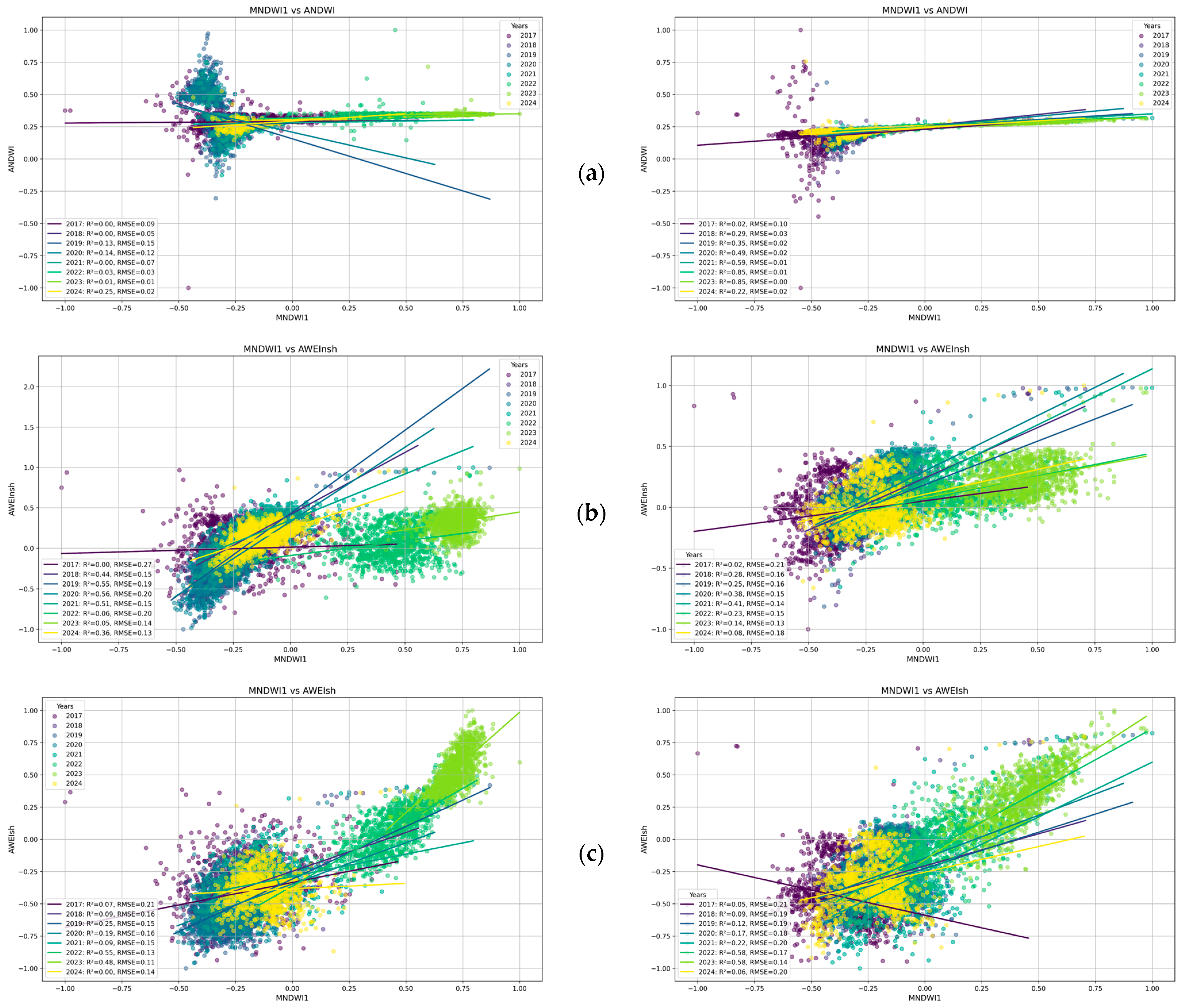
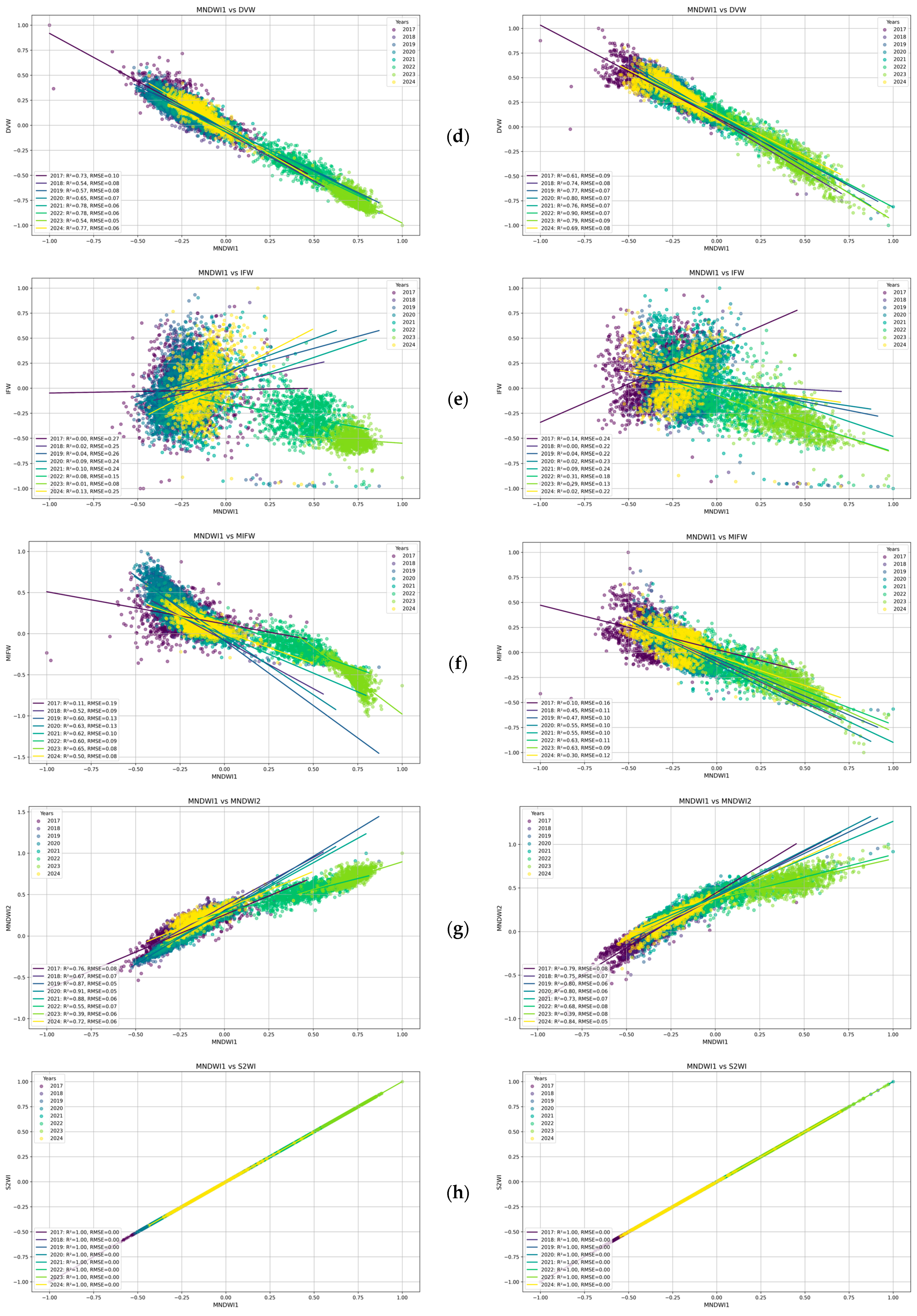
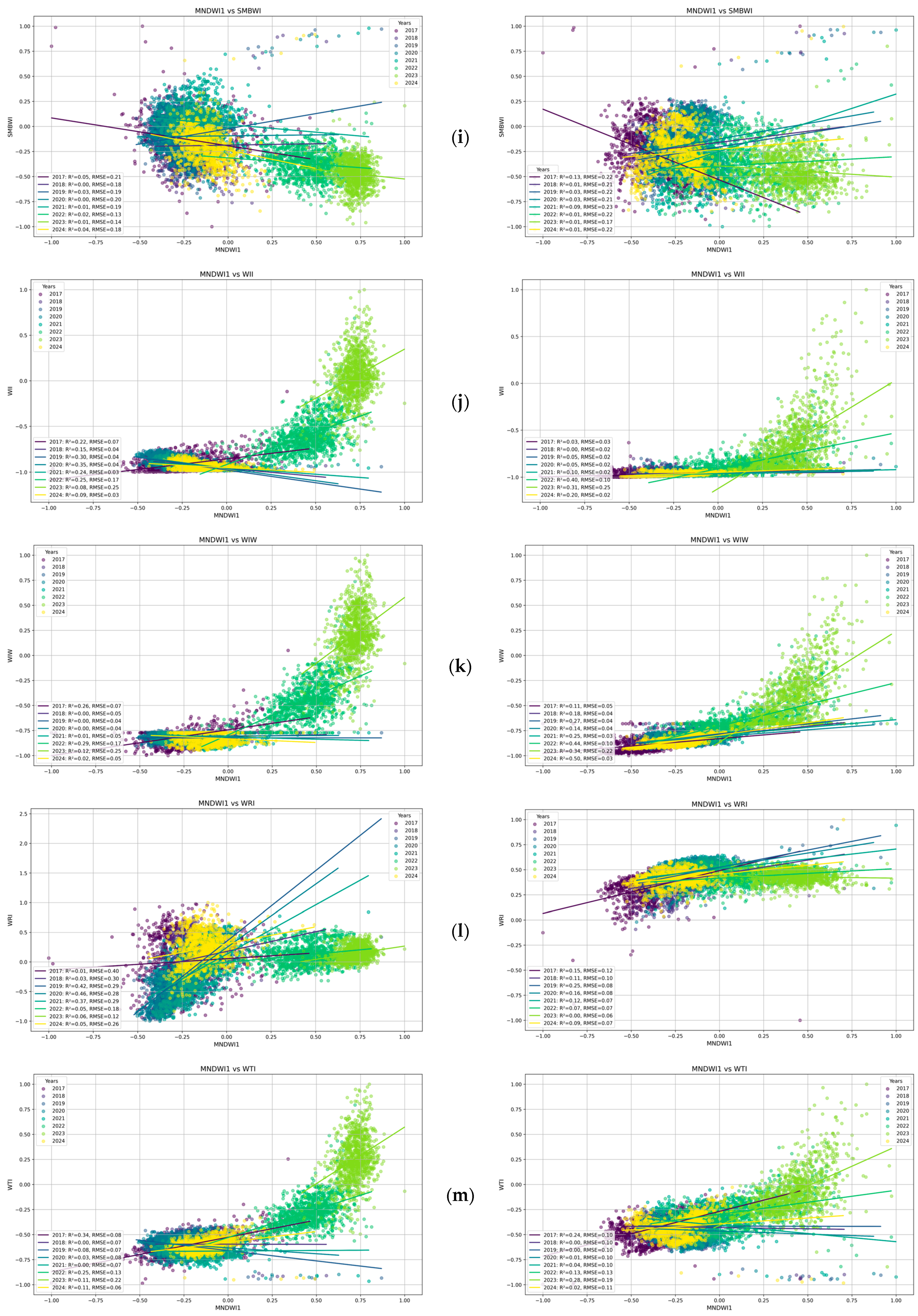
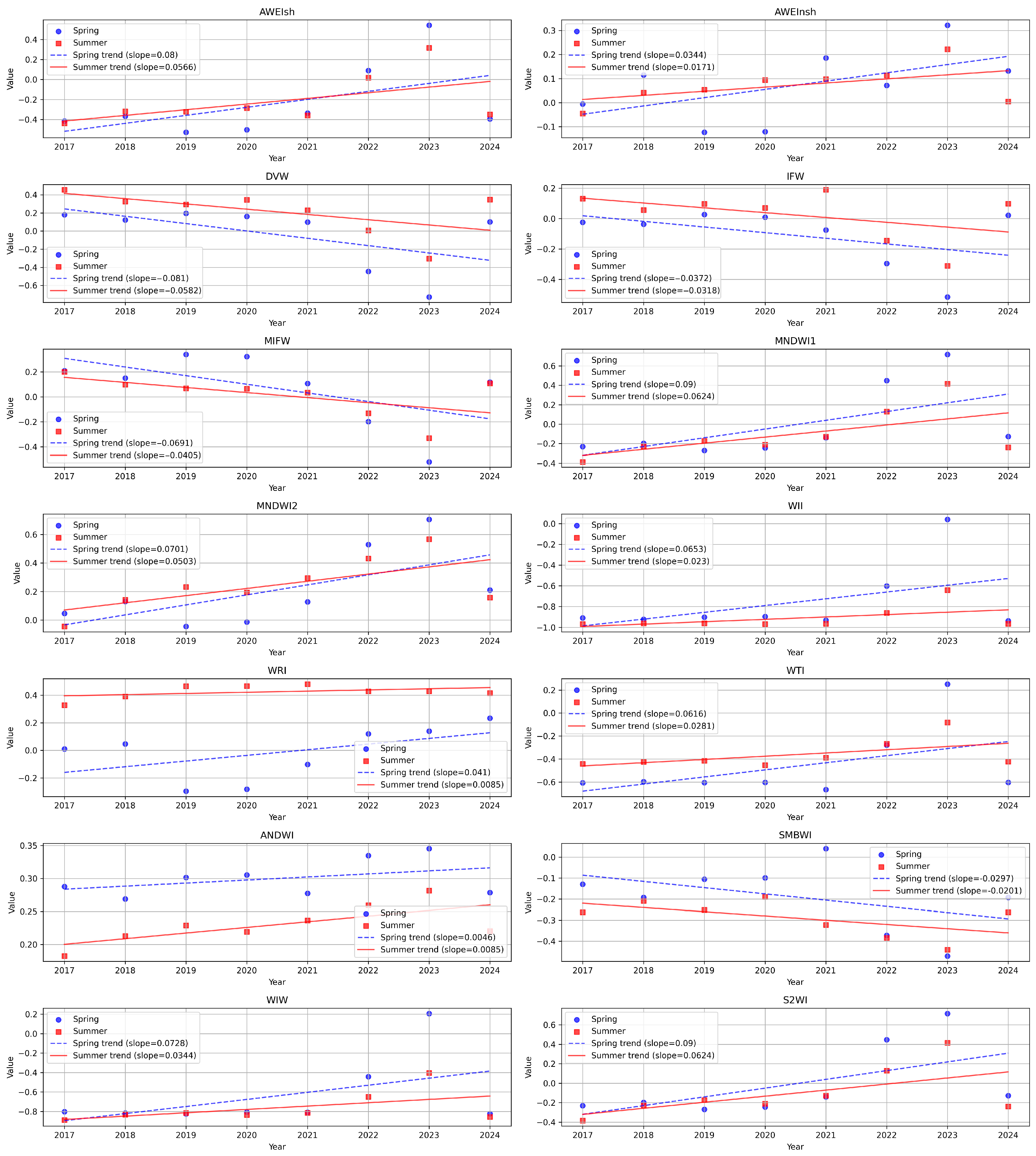
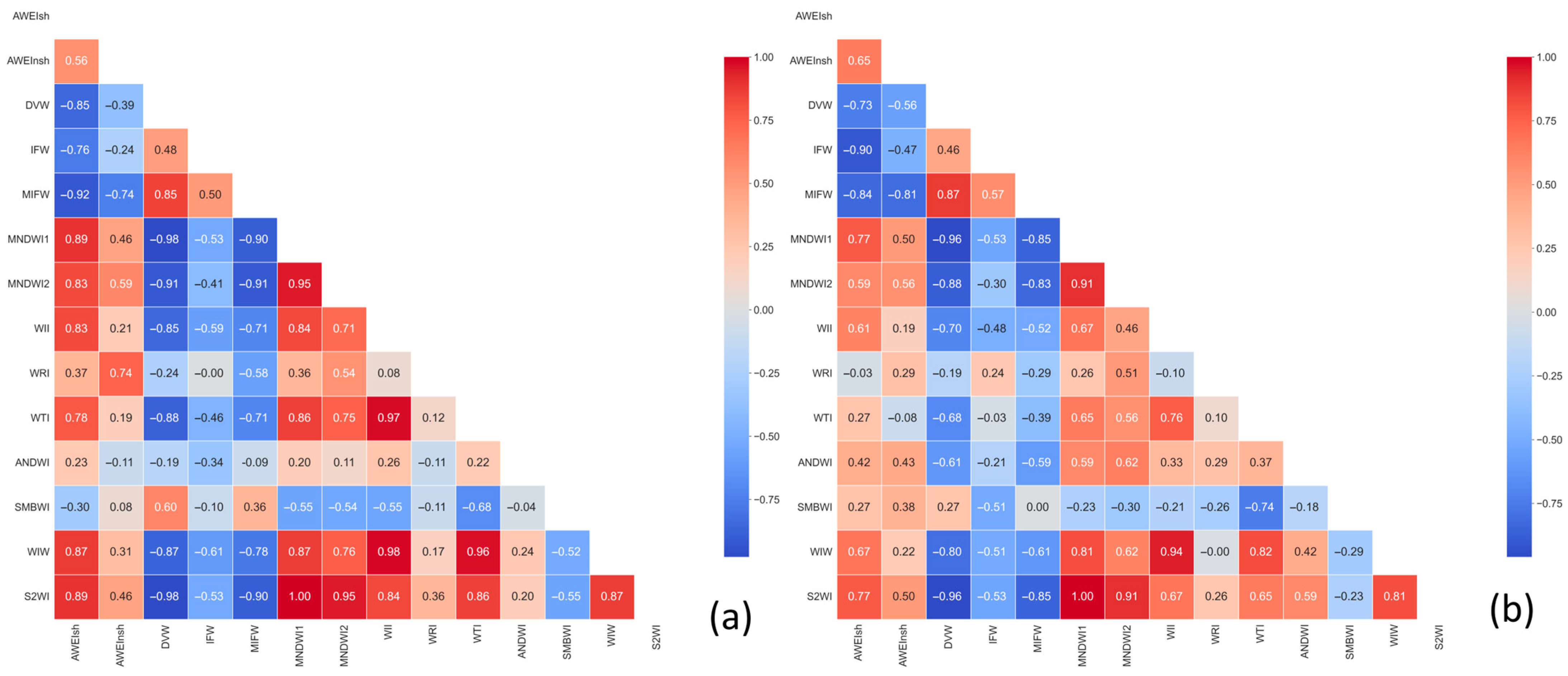
3.1. Trend Analysis and Correlation Relationship

To assess temporal dynamics of water presence and surface wetness, a set of water-related spectral indices was analyzed for seasonal trends between 2017 and 2024, based on spring and summer mean values. Linear regression was applied to estimate the direction and strength of change (slope) for each index–season combination (Figure 2).

Some indices showed opposite trends between spring and summer, reflecting season-specific hydrological dynamics. DVW decreasing in both seasons (spring: −0.081, summer: −0.0723), suggesting a steady decline in vegetation–water contrast, potentially due to drier vegetation or reduced water extent. IFW decreases in both seasons, with the spring decrease (−0.0372) being slightly stronger than the summer decrease (−0.0318), indicating a slight change in the contrast between the green and near-infrared ranges, possibly due to drying or turbidity. The spring trend of MIFW is nearly flat (−0.0691), and the summer shows a slight decline (−0.046), implying stability or slight drying of moist surfaces. Minimal trend of ANDWI (spring: −0.046, summer: −0.0085), indicating relatively stable separation of water vs. vegetation classes.

A decrease in WRI trends from spring to summer indicates a decrease in surface water or a decrease in its visibility. Positive but declining values indicate that water is present, but its area or transparency is decreasing. Like WRI, WTI trend values decrease from spring to summer. This confirms the trend toward drying or reduced surface moisture in summer compared to spring. SMBWI values are negative in both seasons, but they increase (become less negative) from spring to summer (from −0.0297 to −0.0201). If more negative SMBWI values indicate the presence of water, then the transition to less negative values may indicate a decrease in the area of water or a change in its characteristics. This may reflect an increase in the dominance of dry or impervious surfaces, or a change in the spectral behavior of water, for example, due to increased turbidity, which makes water less “shadowy” or more “bright” in the spectral range.

Spring trends are generally stronger (higher slope magnitudes) than summer trends for most indices, suggesting that inter-annual hydrological variability may be more pronounced in spring. Indices using green and SWIR bands (e.g., MNDWI, WIW, S2WI) appear to be more responsive to surface water changes, while ratio-based indices like WRI or entropy-augmented indices (e.g., ANDWI, SMBWI) show greater inter-annual noise and less directional change. The persistent increase in NDWI-type indices suggests a gradual increase in visible water features or improved vegetation moisture retention in wetlands.

Based on the obtained spectral indices for the period from 2017 to 2024, we have obtained the following relation (Figure A1). The matrix of correlation relationships for the entire period of observation for the spring and summer seasons is presented in Figure 3.

The correlation matrices obtained for a set of 14 specialized spectral indices related to water bodies for the spring (Figure 3a) and summer (Figure 3b) seasons permit an in-depth analysis of their interrelationships and seasonal dynamics. The objective of this analysis is to identify stable and changing correlation patterns that reflect various aspects of remote monitoring of water resources.

The observed correlation patterns and their seasonal changes indicate different sensitivity of the spectral indices to various states and characteristics of water bodies and adjacent areas.

The group of indices AWEI_sh, MNDWI1, MNDWI2, WII, WIW, and S2WI have been shown to demonstrate consistent high positive correlations, thus confirming their effectiveness in detecting open water surfaces. The perfect correlation of MNDWI1 and MNDWI2 confirms their identity or direct linear dependence, thus rendering the use of both simultaneously redundant. The DVW, MIFW, and IFW indices have been shown to exhibit a strong negative correlation with the aforementioned “open water” group. This phenomenon may be indicative of their sensitivity to characteristics antithetical to clear water, such as elevated turbidity, the presence of dense aquatic vegetation (e.g., duckweed for IFW/MIFW), or the characterization of the state of drainage or water stress (for DVW).

The observed decline in the correlation strength of AWEI_sh, WII, and WTI with other open water indices during summer months may be attributable to alterations in water quality, such as increased turbidity and algal blooms, or the proliferation of surface and floating vegetation. These factors have the capacity to contaminate the spectral signal of uncontaminated water, exerting an effect on diverse indices in disparate ways. For instance, WTI may exhibit divergent responses to alterations in water conditions during the summer months if it is associated with turbidity.

The transition of ANDWI from a weak to moderate positive correlation with open water indices during the summer months is of significance. This may be indicative of an increase in the prevalence of conditions to which ANDWI is sensitive (e.g., certain depths, sediment types, specific aquatic vegetation) during the summer months, or of a shift in its spectral response to that of other open water indices.

The weakening of the WRI relationship with AWEI_nsh in summer may be indicative of the fact that AWEI_nsh in spring may have been capturing wet floodplains with young vegetation, while in summer, these indices respond to different sites. The observed shift in SMBWI correlations signifies a modification in its interaction with other water conditions, contingent on the season (e.g., open wet soil in spring versus dense vegetation and disparate moisture regimes in summer).

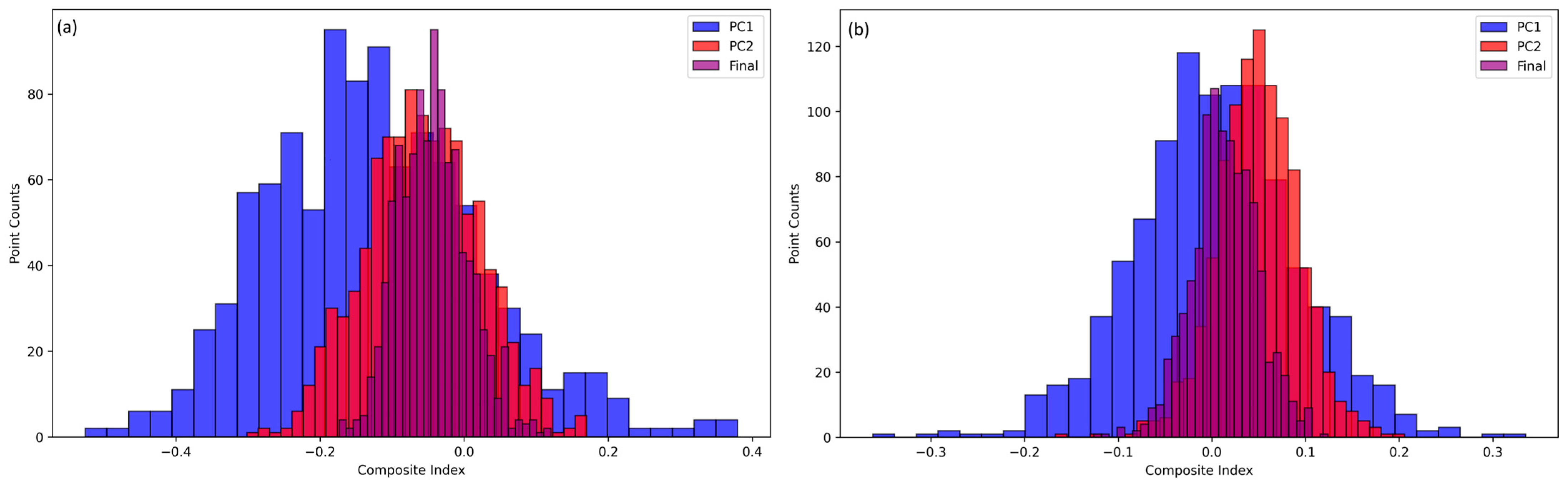
3.2. Principal Component Analysis (PCA)

The impact of spectral indices on principal components (PCA) was analyzed for the entire set of spectral index values obtained for the period 2017–2024. The ensuing findings are presented in graphical form in Figure 4, (a) for spring and (b) for summer seasons.

The objective of this study is to analyze the variability of water spectral indices using the principal component analysis (PCA) method for the spring and summer periods. The utilization of PCA facilitates the reduction of multidimensional data to a smaller number of synthetic variables (principal components) that provide a comprehensive explanation of the observed variance. The objective of the analysis is to identify dominant patterns and seasonal differences in the correlations between individual spectral indices and the resulting components.

In the spring period, the first principal component (PC1) demonstrates high absolute values of correlation coefficients with a number of key water spectral indices, such as IFW, MNDWI1, and WIW. This finding suggests that these indices play a pivotal role in elucidating the variability of the data during the spring period (Figure 5a). The existence of both positive and negative correlations suggests that certain indices may be indicative of complementary aspects of water processes, such as changes in humidity, hydrodynamic processes, or variations in the light reflectance properties of water surfaces. The results obtained thus far suggest that the spring season is characterized by active hydrological dynamics [54], where the recovery of water resources after the winter period is accompanied by distinct changes in spectral characteristics.

During the summer months, a transition in the correlation structure between spectral indices and principal components becomes evident. Although PC1 remains the principal component, the characterization of its influence is somewhat modified: some indices that dominated in the spring period have a weaker influence on PC1 in the summer season, while their contribution is transferred to the following components, in particular PC2 and PC3 (Figure 5b).

This change may be attributed to physiological and hydrological processes inherent in the summer period, including increased evaporation, reduced water resources, and changes in vegetation around water bodies. Therefore, the distribution of the contribution of individual spectral indices to the variability of the data indicates an adaptive response of the system to high-temperature stress and structural alterations of water bodies under summer conditions.

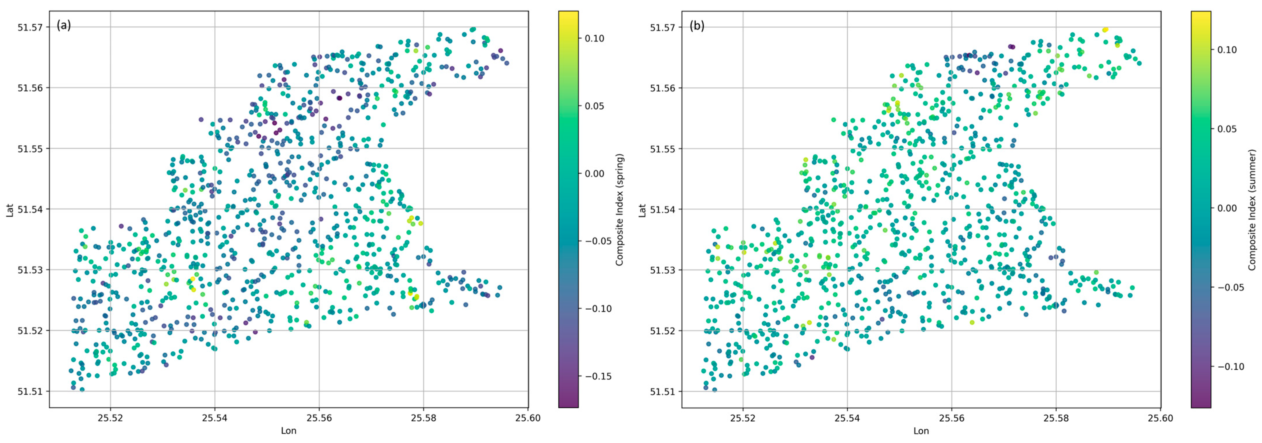
3.3. Composite Index

In accordance with the methodology delineated in Section 2.3.4, the integral composite indices (CIs) were computed in order to characterize the general trend of long-term changes in the state of water surfaces in the Cheremsky Nature Reserve for the period 2017–2024, specifically for the spring and summer seasons. This index is employed to aggregate the normalized trends of 14 spectral indices of water surfaces; these are weighted according to their contribution to the first two principal components (abbreviated here as PC1 and PC2) and the influence coefficients of these components. The principal component analysis (PCA) of the normalized trends of the 14 spectral indices demonstrated that the first two principal components (PC1 and PC2) explained 64.2%/57.3% and 14.2/18.2% of the total variation in the data, respectively, for the spring/summer seasons (Figure 5). The loadings of the original indices on these two components were used to calculate individual weights for PC1 ($w_i^{PC1}$) and PC2 ($w_i^{PC2}$).

The formation of a composite index necessitated the calculation of the coefficients of influence for the first (α) and second (β) principal components, which were determined to be 0.357 and 0.240, respectively.

The composite index for each point of a particular season was calculated as a weighted sum of the normalized trends (${\mathrm{X}}_{\mathrm{n}\mathrm{o}\mathrm{r}{\mathrm{m}}_{\mathrm{s}}\mathrm{l}\mathrm{o}\mathrm{p}\mathrm{e},\mathrm{i}}$) of all 14 spectral indices using combined weights:

$$\mathrm{C}\mathrm{I}={\sum }_{\mathrm{i}=1}^{14}{\mathrm{w}}_{\mathrm{i}}^{\mathrm{c}\mathrm{o}\mathrm{m}\mathrm{b}}·{\mathrm{X}}_{\mathrm{n}\mathrm{o}\mathrm{r}{\mathrm{m}}_{\mathrm{s}}\mathrm{l}\mathrm{o}\mathrm{p}\mathrm{e},\mathrm{i}}$$

(3)

The equations for each season (${CI}_{spring}$ and ${CI}_{summer}$) based on the calculated combined weights are (4) and (5):

$$\begin{array}{cc}{\mathrm{C}\mathrm{I}}_{\mathrm{s}\mathrm{p}\mathrm{r}\mathrm{i}\mathrm{n}\mathrm{g}}=& 0.024·AWEIsh+0.029·AWEInsh+0.032·DVW+0.017·IFW\\ & \hspace{1em}\hspace{1em} +0.038·MIFW+0.046·MNDWI1+0.059·MNDWI2\\ & \hspace{1em}\hspace{1em} +0.023·WII+0.044·WRI+0.025·WTI+0.017·ANDWI\\ & \hspace{1em}\hspace{1em} +0.019·SMBWI+0.035·WIW+0.046·S2WI\end{array}$$

(4)

$$\begin{array}{cc}{\mathrm{C}\mathrm{I}}_{\mathrm{s}\mathrm{u}\mathrm{m}\mathrm{m}\mathrm{e}\mathrm{r}}=& 0.057·AWEIsh+0.028·AWEInsh+0.078·DVW+0.052·IFW\\ & \hspace{1em}\hspace{1em} +0.040·MIFW+0.062·MNDWI1+0.062·MNDWI2\\ & \hspace{1em}\hspace{1em} +0.008·WII+0.016·WRI+0.042·WTI+0.023·ANDWI\\ & \hspace{1em}\hspace{1em} +0.046·SMBWI+0.020·WIW+0.062·S2WI\end{array}$$

(5)

The distribution of values for the designated study area is illustrated in Figure 6. The mean values of the indices are −0.043 and 0.14, with standard deviations of −0.043 ± 0.048 and 0.014 ± 0.035 for the spring and summer seasons, respectively.

Recent remote sensing studies have used similar composite or multi-metric indices to synthesize wetland condition [55] and shown that such indices facilitate spatial targeting and trend analysis for wetland management [56].

A PCA-derived composite index (CI) of multiple spectral water and vegetation indicators yields a single wetland “health” metric that is far easier for managers to interpret than dozens of separate time series. Spatially, the CI highlights zones of concern versus resilience: for example, areas with persistently low or declining CI (reflecting simultaneous drops in water extent and biomass) mark wetlands under stress, whereas clusters of high or rising CI emerge as “hot spots” of healthy or recovering wetlands [56].

The spatial distribution of the values of ${CI}_{spring}$ and ${CI}_{summer}$ (Figure 7) allows us to visualize the areas with the most pronounced positive and negative trends in water regime changes for both periods.

The values obtained provide an indication of the relative stability of the water regime during the study period, with the averaging process conducted across all indices and seasons.

4. Discussion

The spectral analysis reveals a gradual increase in water-sensitive index values in both spring and summer for several robust indices (MNDWI1/2, WIW, S2WI), indicating expanding or more persistent surface water bodies from 2017 to 2024. However, certain indices show declining trends, particularly in vegetation or turbidity-sensitive contexts (e.g., WRI, SMBWI), potentially signaling localized water loss or spectral interference from land cover changes. The results underscore the importance of multi-index monitoring to comprehensively capture seasonal and long-term hydrological dynamics in complex wetland systems.

The analysis of correlation matrices of specialized water indices revealed the presence of both stable and seasonally dependent relationships.

There is a core of indices (MNDWI1, MNDWI2, S2WI, WIW, partially AWEI_sh, and WII) that are consistently highly correlated with each other and are reliable indicators of open water. The redundancy of some of them (MNDWI1/MNDWI2) should be taken into account in practical applications.

The DVW, MIFW, and IFW indices consistently show a negative correlation with open water indices, indicating their potential usefulness for detecting alternative states of the water surface (e.g., high concentration of suspended solids, presence of floating vegetation) or adjacent areas.

There is a significant seasonal variation in the strength and sometimes in the direction of correlations for a number of indices (in particular, ANDWI, WTI, WRI, SMBWI, as well as in the interrelationships of AWEI_sh and WII with others). This emphasizes their differential sensitivity to changes in water conditions, aquatic and riparian vegetation, and possibly water quality during the growing season.

The obtained results emphasize the need for careful selection of spectral indices depending on the specific tasks of water resources monitoring, the season of research, and the expected characteristics of water bodies. Seasonal dynamics of correlations should be taken into account when building long-term models and interpreting time series of remote sensing data. A comparative analysis of the PCA results for the spring and summer seasons indicates that there are significant seasonal differences in the structure of the relationships of water spectral indices. The findings of the present study demonstrate that the implementation of the PCA method in the analysis of water spectral indices facilitates the effective detection of seasonal variability and structural changes in aquatic systems. It is evident that the conclusions of this study are of considerable practical importance for the purposes of further hydrological monitoring, effective water resources management, and the development of effective climate change adaptation measures.

The composite index (CI) of long-term trends of water surfaces, calculated on the basis of 14 spectral indices and weighted by PCA, as proposed in this study, provides an integrated assessment of the dynamics of the water regime of the Cheremsky Nature Reserve. The employment of PCA to ascertain the weights facilitated an objective accounting of the contribution of each index and the reduction in data redundancy, a method that aligns with approaches utilized in other studies to evaluate the state of the environment and agricultural sustainability [52,53,54]. The identification of spatial patterns of positive and negative CI values indicates heterogeneity of changes in the water regime within the reserve. This heterogeneity may be related to local hydromorphological features, vegetation cover, and anthropogenic impact on adjacent territories, despite the reserve’s status.

A similar approach to creating composite indices for monitoring water resources or wetlands has been utilized previously [57,58]. For instance, Amani et al. [20] also employed multi-source optical data and spectral indices to analyze wetlands, although their focus lay in classification rather than a composite trend index. A comparison with similar works demonstrates that the chosen methodology is contemporary and suitable for addressing the tasks. However, in contrast to numerous studies that concentrate on contemporary water bodies, our CI characterizes the dynamics (trend) of these changes, which is imperative for evaluating long-term ecological processes. In temporal terms, positive CI trends imply net improvement in wetland condition (e.g., increased inundation or vegetative cover), whereas negative trends signal degradation (drying or vegetation loss). This clarity lets decision-makers translate CI maps directly into action: regions with low or falling CI can be prioritized for conservation or restoration (e.g., rewetting, buffer enhancement), while stable or high-CI areas may be treated as management successes or reference benchmarks [56]. Crucially, CI can also track intervention outcomes over time: an upward shift in CI in a restored or protected wetland signals effective management, whereas a stagnant or declining CI would prompt adaptive measures [55,59]. For instance, a landscape-health CI applied to China’s mangrove reserves showed that over 80% of sites had significant CI increases under protection, demonstrating the index’s value in quantifying conservation success [59].

The seasonal variability of both individual indices and the structure of the principal components observed in this study emphasize the complexity of wetlands monitoring. As Li et al. [19] previously observed, analogous seasonal effects were identified during the monitoring of the hydrological dynamics of seasonally flooded wetlands in Spain. This finding underscores the necessity for a distinct analysis for varying seasons or the creation of seasonally adapted indices.

The utilization of Sentinel-2 data, with a resolution of 10–20 m, signifies a substantial enhancement over the capabilities of Landsat. Nevertheless, it might not be adequate to discern very small water bodies or narrow waterways within the dense vegetation characteristic of the Cheremsky Reserve. This limitation is characteristic of a significant number of studies of wetlands that employ satellite data [6].

Despite the implementation of cloud masking and median compositing techniques to mitigate their impact, residual atmospheric effects or inadequately removed clouds/cloud shadows could potentially compromise the precision of spectral index calculations, particularly during short-term periods or when analyzing indices that are particularly sensitive to minimal variations in reflectance.

The set of 14 water indices is a fairly representative sample, but does not exhaust the variety of existing approaches. Furthermore, it should be noted that certain indices may demonstrate comparable spectral sensitivity (a phenomenon that is partially offset by PCA). Additionally, specific conditions (for example, water blooms and floating vegetation) may be interpreted in a divergent manner by different indices.

5. Conclusions

Recent studies have significantly expanded the understanding of the application of spectral indices in wetland monitoring, especially using Sentinel-2 data. Spectral indices have been demonstrated to serve as superior predictors for the evaluation of biophysical variables, including above-ground biomass and organic carbon. A multitude of comparative studies have confirmed that modified water indices, such as the MNDWI, frequently exhibit superior performance in accurately distinguishing water surfaces and water/vegetation mixtures when compared to the NDWI and the WRI. This enhanced accuracy can be attributed to the heightened sensitivity of the SWIR bands to moisture. Research has demonstrated that the utilization of composite indices can yield superior outcomes in the identification of wetland flooding when compared with the application of individual indices.

The contribution of Sentinel-2 data is significant due to its high spatial and temporal resolution, which allows for detailed mapping of vegetation and water bodies. While Sentinel-2 “red edge” indices have demonstrated their efficacy, they frequently exhibit a temporal delay in their significance relative to other spectral indices and bands, such as SWIR. The integration of spectral indices with Synthetic Aperture Radar (SAR) data, topographic models, and machine learning algorithms has been demonstrated to enhance the accuracy of wetland mapping, particularly in complex and dynamic ecosystems. Subsequent research endeavors should prioritize the development of advanced methodologies that consider the dynamic characteristics of wetlands. These methodologies should aim to enhance precision and broaden the scope of monitoring capabilities, particularly through the utilization of long-term time series and phenological attributes.

A composite indicator was developed for the spring and summer seasons, based on normalized trends and weighting coefficients obtained from principal component analysis (PCA). This indicator is an effective summary of information regarding the water regime, providing a comprehensive depiction of its dynamics and facilitating more nuanced interpretation of complex changes. The developed CI demonstrated clear seasonal differences, emphasizing the importance of considering the water regime in the context of different hydrological seasons. This finding underscores the necessity for a nuanced strategy that incorporates a year-round monitoring and management approach for wetlands. The findings of this study constitute a significant addition to the body of knowledge concerning the dynamics of water resources in the Ukrainian Polissya, thereby substantiating the efficacy of remote sensing and geoinformation systems, particularly Google Earth Engine, in facilitating the long-term monitoring of wetlands. The composite indicator developed can serve as an effective tool for assessing the state of the water regime, for identifying critical changes in the system, and for supporting decision-making in the realms of nature conservation and water resource management.

Subsequent studies could entail the validation of results derived from ground-based data, the extension of time series to facilitate longer-term forecasts, and the incorporation of other satellite data, such as radar, to circumvent constraints associated with cloud cover.

Direct validation of the obtained trends and values of the composite index using ground-based data on water level, flooded area, or other hydrological parameters within the Cheremsky Reserve was limited due to the lack of such systematic observations. As asserted by Kaplan and Avdan [7], such validation is imperative in order to verify the precision of remote estimates.

In order to facilitate further development and refinement of the proposed methodology and to enhance comprehension of the processes within the Cheremsky Reserve, the following areas require delineation:

• The creation of a composite index combining water and vegetation data is presented. The development of a CI that simultaneously considers trends in both water surfaces and vegetation condition (e.g., health, density, ferrology) can provide a more comprehensive understanding of ecological changes in bogs. This is of particular pertinence in regions where hydrological processes are inextricably linked to vegetation dynamics, a phenomenon that is exemplified by the Cheremsky Reserve. A range of studies have adopted an approach that combines water and vegetation metrics in order to assess droughts or ecosystem health (for example, Kogan, 1995—VHI [60]; AghaKouchak et al., 2015—MWDI [61]).
• The investigation of the correlations and time lags between changes in water indices and vegetation indices can facilitate the identification of cause-and-effect relationships. For instance, it can be determined how changes in water levels affect vegetation productivity, or conversely, how vegetation succession affects water regimes.
• The utilization of commercial satellite data (e.g., PlanetScope, WorldView) with very high resolution, or radar sensor data (e.g., Sentinel-1), which are insensitive to cloud cover and can penetrate vegetation, has the potential to enhance the precision and reliability of monitoring, particularly in the context of detecting water beneath vegetation [7,62].
• In addition to linear trends, breakpoint analysis methods (e.g., BFAST) should be considered in order to identify abrupt changes in water index dynamics. Such changes may be associated with extreme events or land use changes.

References

1. Solovey, T. Wetlands of the Volhynian Polissia (Western Ukraine): Classification, Natural Conditions of Distribution and Spatial Difference. Geol. Q. 2019, 63, 139–149. [Google Scholar] [CrossRef]
2. Convention on Wetlands Global. Guidelines for Peatland Rewetting and Restoration; Convention on Wetlands Global: Gland, Switzerland, 2021. [Google Scholar]
3. Ramsar Convention Secretariat. The Ramsar Convention Manual: A Guide to the Convention on Wetlands (Ramsar, Iran, 1971), 6th ed.; Ramsar Convention Secretariat: Gland, Switzerland, 2007. [Google Scholar]
4. Zhang, S.; Na, X.; Kong, B.; Wang, Z.; Jiang, H.; Yu, H.; Zhao, Z.; Li, X.; Liu, C.; Dale, P. Identifying Wetland Change in China’s Sanjiang Plain Using Remote Sensing. Wetlands 2009, 29, 302–313. [Google Scholar] [CrossRef]
5. Frohn, R.C.; Reif, M.; Lane, C.; Autrey, B. Satellite Remote Sensing of Isolated Wetlands Using Object-Oriented Classification of Landsat-7 Data. Wetlands 2009, 29, 931–941. [Google Scholar] [CrossRef]
6. Ozesmi, S.L.; Bauer, M.E. Satellite Remote Sensing of Wetlands. Wetl. Ecol. Manag. 2002, 10, 381–402. [Google Scholar] [CrossRef]
7. Kaplan, G.; Avdan, U. Monthly Analysis of Wetlands Dynamics Using Remote Sensing Data. ISPRS Int. J. Geo-Inf. 2018, 7, 411. [Google Scholar] [CrossRef]
8. Sentinel-2—Sentinel Online. Available online: https://sentinels.copernicus.eu/copernicus/sentinel-2 (accessed on 13 March 2025).
9. Gorelick, N.; Hancher, M.; Dixon, M.; Ilyushchenko, S.; Thau, D.; Moore, R. Google Earth Engine: Planetary-Scale Geospatial Analysis for Everyone. Remote Sens. Environ. 2017, 202, 18–27. [Google Scholar] [CrossRef]
10. Belloli, T.F.; Guasselli, L.A.; Kuplich, T.M.; Fernando, L.; Ruiz, C.; Carvalho De Arruda, D.; Balsamo Etchelar, C.; Simioni, J.D. Estimation of Aboveground Biomass and Carbon in Palustrine Wetland Using Bands and Multispectral Indices Derived from Optical Satellite Imageries PlanetScope and Sentinel-2A. J. Appl. Remote Sens. 2022, 16, 034516. [Google Scholar] [CrossRef]
11. Ade, C.; Khanna, S.; Lay, M.; Ustin, S.L.; Hestir, E.L. Genus-Level Mapping of Invasive Floating Aquatic Vegetation Using Sentinel-2 Satellite Remote Sensing. Remote Sens. 2022, 14, 3013. [Google Scholar] [CrossRef]
12. Yu, H.; Li, S.; Liang, Z.; Xu, S.; Yang, X.; Li, X. Multi-Source Remote Sensing Data for Wetland Information Extraction: A Case Study of the Nanweng River National Wetland Reserve. Sensors 2024, 24, 6664. [Google Scholar] [CrossRef]
13. Salas, E.A.L.; Kumaran, S.S.; Bennett, R.; Willis, L.P.; Mitchell, K. Machine Learning-Based Classification of Small-Sized Wetlands Using Sentinel-2 Images. AIMS Geosci. 2024, 10, 62–79. [Google Scholar] [CrossRef]
14. Usman, M.; Chua, L.H.; Irvine, K.N.; Teang, L. Estimating Water Surface Elevation for a Wetland Using Integrated Multi-Sourced Remote Sensing Data. Wetl. Ecol. Manag. 2025, 33, 20. [Google Scholar] [CrossRef]
15. Jamali, A.; Mahdianpari, M.; Mohammadimanesh, F.; Brisco, B.; Salehi, B. A Synergic Use of Sentinel-1 and Sentinel-2 Imagery for Complex Wetland Classification Using Generative Adversarial Network (GAN) Scheme. Water 2021, 13, 3601. [Google Scholar] [CrossRef]
16. Solovey, T. Flooded Wetlands Mapping from Sentinel-2 Imagery with Spectral Water Index: A Case Study of Kampinos National Park in Central Poland. Geol. Q. 2020, 64, 492–505. [Google Scholar] [CrossRef]
17. Tajadod, M.J.; Haghighi Khomami, M.; Modaberi, H.; Panahandeh, M. Integrating Sentinel 1 and 2 Satellite Data with Spectral Indices to Improve Classification Methods (Anzali Wetland). Environ. Sci. 2024, 22, 389–406. [Google Scholar] [CrossRef]
18. Chaudhary, R.K.; Puri, L.; Acharya, A.K.; Aryal, R. Wetland Mapping and Monitoring with Sentinel-1 and Sentinel-2 Data on the Google Earth Engine. J. For. Nat. Resour. Manag. 2023, 3, 1–21. [Google Scholar] [CrossRef]
19. Li, L.; Vrieling, A.; Skidmore, A.; Wang, T.; Muñoz, A.R.; Turak, E. Evaluation of MODIS Spectral Indices for Monitoring Hydrological Dynamics of a Small, Seasonally-Flooded Wetland in Southern Spain. Wetlands 2015, 35, 851–864. [Google Scholar] [CrossRef]
20. Amani, M.; Salehi, B.; Mahdavi, S.; Brisco, B. Spectral Analysis of Wetlands Using Multi-Source Optical Satellite Imagery. ISPRS J. Photogramm. Remote Sens. 2018, 144, 119–136. [Google Scholar] [CrossRef]
21. Lyalko, V.; Zholobak, G.; Dugin, S.; Sybirtseva, O.; Golubov, S.; Dorofey, Y.; Polishchuk, O. Experimental Research of the Carbon Circle Features in “Atmosphere–Vegetation” System over the Wetland Area within the Forest–Steppe Zone in Ukraine Using Remote Spectro- and Gasometry under the Global Climate Changes. Ukr. J. Remote Sens. 2020, 24, 15–23. [Google Scholar] [CrossRef]
22. Azimov, O.; Tomchenko, O.; Shevchenko, O.; Dorofey, Y. Satellite Monitoring of the Natural and Technogenic Events on the Left-Bank Pripyat Reclamation System of the Chornobyl Exclusion Zone. In Proceedings of the XVI International Scientific Conference “Monitoring of Geological Processes and Ecological Condition of the Environment”, Kyiv, Ukraine, 15–18 November 2022; pp. 1–6. [Google Scholar]
23. Lyalko, V.I.; Shportiuk, Z.M.; Sibirtseva, O.M.; Dugin, S.S. Research of Hyperspectral Red Edge Indices for Vegetation Cover Change Detection over the Oil Field Using Spectrometric Survey Data. Geol. Zhurnal 2014, 3, 95–103. [Google Scholar]
24. Lyalko, V.I.; Popov, M.O. (Eds.) Multispectral Methods of Earth Remote Sensing in Land Use Tasks; Naukova Dumka: Kyiv, Ukraine, 2006. [Google Scholar]
25. Trofymchuk, O.M.; Trisyuk, V.M.; Anpilova, E.S.; Butenko, O.S.; Vishnyakov, V.Y.; Zagorodnia, S.A.; Klymenko, V.I.; Klochko, T.O.; Krasovska, I.G.; Kreta, D.L.; et al. Geoinformation Studies of Water Ecosystems in Ukraine: Monitoring and Forecasting; Suprun V.P.: Ivano-Frankivsk, Ukraine, 2022; ISBN 978-617-8128-10-4. [Google Scholar]
26. Konishchuk, V.V. Estimation of Difersity Ecosystems Cheremskyi Natural Reserve on the Basis of Cartographical Modelling, A Manuscript. Ph.D. Dissertation, National Taras Shevchenko University, Kyiv, Ukraine, 2006. Available online: https://uacademic.info/ua/document/0406U000865 (accessed on 13 March 2025).
27. Martyniuk, V.; Korbutiak, V.; Hopchak, I.; Kovalchuk, I.; Zubkovych, I. Methodology for Assessing the Geoecological State of Landscape-Lake Systems and Their Cartographic Modelling (Case Study of Lake Bile, Rivne Nature Reserve, Ukraine). Baltica 2023, 36, 13–29. [Google Scholar] [CrossRef]
28. Kovalchuk, I.P.; Martyniuk, V.A. Methodology and Experience of Landscape-Limnological Research into Lake-Basin Systems of Ukraine. Geogr. Nat. Resour. 2015, 36, 305–312. [Google Scholar] [CrossRef]
29. Pavlovska, T.S.; Kovalchuk, I.P. Geomorphology: Textbook for Students of Higher Education Institutions; VezhaDruk: Lutsk, Ukraine, 2022. [Google Scholar]
30. Cheremske Bog|Ramsar Sites Information Service. Available online: https://rsis.ramsar.org/ris/2272 (accessed on 10 March 2025).
31. Harmonized Sentinel-2 MSI: MultiSpectral Instrument, Level-2A (SR)|Earth Engine Data Catalog|Google for Developers. Available online: https://developers.google.com/earth-engine/datasets/catalog/COPERNICUS_S2_SR_HARMONIZED#terms-of-use (accessed on 13 March 2025).
32. Feyisa, G.L.; Meilby, H.; Fensholt, R.; Proud, S.R. Automated Water Extraction Index: A New Technique for Surface Water Mapping Using Landsat Imagery. Remote Sens. Environ. 2014, 140, 23–35. [Google Scholar] [CrossRef]
33. Acharya, T.D.; Subedi, A.; Lee, D.H. Evaluation of Water Indices for Surface Water Extraction in a Landsat 8 Scene of Nepal. Sensors 2018, 18, 2580. [Google Scholar] [CrossRef] [PubMed]
34. Jiang, H.; Feng, M.; Zhu, Y.; Lu, N.; Huang, J.; Xiao, T. An Automated Method for Extracting Rivers and Lakes from Landsat Imagery. Remote Sens. 2014, 6, 5067–5089. [Google Scholar] [CrossRef]
35. Gond, V.; Bartholomé, E.; Ouattara, F.; Nonguierma, A.; Bado, L. Surveillance et Cartographie Des Plans d’eau et Des Zones Humides et Inondables En Régions Arides Avec l’instrument VEGETATION Embarqué Sur SPOT-4. Int. J. Remote Sens. 2004, 25, 987–1004. [Google Scholar] [CrossRef]
36. Crippen, R.E. Calculating the Vegetation Index Faster. Remote Sens. Environ. 1990, 34, 71–73. [Google Scholar] [CrossRef]
37. McFeeters, S.K. The Use of the Normalized Difference Water Index (NDWI) in the Delineation of Open Water Features. Int. J. Remote Sens. 1996, 17, 1425–1432. [Google Scholar] [CrossRef]
38. Adell, C.; Puech, C. Will the Spatial Analysis of Water Maps Extracted by Remote Satellite Detection Allow Locating the Footprints of Hunting Activity in the Camargue? Bull.—Soc. Fr. Photogramm. Teledetect. 2003, 171, 76–86. [Google Scholar]
39. Davranche, A.; Poulin, B.; Lefebvre, G. Mapping Flooding Regimes in Camargue Wetlands Using Seasonal Multispectral Data. Remote Sens. Environ. 2013, 138, 165–171. [Google Scholar] [CrossRef]
40. Xu, H. Modification of Normalised Difference Water Index (NDWI) to Enhance Open Water Features in Remotely Sensed Imagery. Int. J. Remote Sens. 2006, 27, 3025–3033. [Google Scholar] [CrossRef]
41. Jones, S.K.; Fremier, A.K.; DeClerck, F.A.; Smedley, D.; Pieck, A.O.; Mulligan, M. Big Data and Multiple Methods for Mapping Small Reservoirs: Comparing Accuracies for Applications in Agricultural Landscapes. Remote Sens. 2017, 9, 1307. [Google Scholar] [CrossRef]
42. Sawetwong, C.; Reungsang, P. Comparison of NDWI, MNDWI1 and MNDWI2 Indices from Sentinel-2 Satellite Images for Extracting Urban Surface Water Bodies in Khon Kaen. J. Appl. Informatics Technol. 2022, 4, 1–12. [Google Scholar] [CrossRef]
43. Feng, M.; Sexton, J.O.; Channan, S.; Townshend, J.R. A Global, High-Resolution (30-m) Inland Water Body Dataset for 2000: First Results of a Topographic–Spectral Classification Algorithm. Int. J. Digit. Earth 2016, 9, 113–133. [Google Scholar] [CrossRef]
44. Potapov, P.V.; Turubanova, S.A.; Tyukavina, A.; Krylov, A.M.; McCarty, J.L.; Radeloff, V.C.; Hansen, M.C. Eastern Europe’s Forest Cover Dynamics from 1985 to 2012 Quantified from the Full Landsat Archive. Remote Sens. Environ. 2015, 159, 28–43. [Google Scholar] [CrossRef]
45. Sharma, R.C.; Durga Rao, K.H.V.; Jagarlapudi, A. Effect of Spatial Resolution on Classification of Wetlands. Asian-Pac. Remote Sens. J. 1996, 8, 47–51. [Google Scholar]
46. Rokni, K.; Ahmad, A.; Selamat, A.; Hazini, S. Water Feature Extraction and Change Detection Using Multitemporal Landsat Imagery. Remote Sens. 2014, 6, 4173–4189. [Google Scholar] [CrossRef]
47. Kameyama, S.; Yamagata, Y.; Nakamura, F.; Kaneko, M. Development of WTI and Turbidity Estimation Model Using SMA—Application to Kushiro Mire, Eastern Hokkaido, Japan. Remote Sens. Environ. 2001, 77, 1–9. [Google Scholar] [CrossRef]
48. Rad, A.M.; Kreitler, J.; Sadegh, M. Augmented Normalized Difference Water Index for Improved Surface Water Monitoring. Environ. Model. Softw. 2021, 140, 105030. [Google Scholar] [CrossRef]
49. Su, Z.; Xiang, L.; Steffen, H.; Jia, L.; Deng, F.; Wang, W.; Hu, K.; Guo, J.; Nong, A.; Cui, H.; et al. A New and Robust Index for Water Body Extraction from Sentinel-2 Imagery. Remote Sens. 2024, 16, 2749. [Google Scholar] [CrossRef]
50. Lefebvre, G.; Davranche, A.; Willm, L.; Campagna, J.; Redmond, L.; Merle, C.; Guelmami, A.; Poulin, B. Introducing WIW for Detecting the Presence of Water in Wetlands with Landsat and Sentinel Satellites. Remote Sens. 2019, 11, 2210. [Google Scholar] [CrossRef]
51. Jiang, W.; Ni, Y.; Pang, Z.; Li, X.; Ju, H.; He, G.; Lv, J.; Yang, K.; Fu, J.; Qin, X. An Effective Water Body Extraction Method with New Water Index for Sentinel-2 Imagery. Water 2021, 13, 1647. [Google Scholar] [CrossRef]
52. Kevin Sinisterra-Solís, N.; Sanjuán, N.; Ribal, J.; Estruch, V.; Clemente, G.; Rozakis, S. Developing a Composite Indicator to Assess Agricultural Sustainability: Influence of Some Critical Choices. Ecol. Indic. 2024, 161, 111934. [Google Scholar] [CrossRef]
53. Melo-Aguilar, C.; Agulles, M.; Jordà, G. Introducing Uncertainties in Composite Indicators. The Case of the Impact Chain Risk Assessment Framework. Front. Clim. 2022, 4, 1019888. [Google Scholar] [CrossRef]
54. Melnyk, O.; Brunn, A. Analysis of Spectral Index Interrelationships for Vegetation Condition Assessment on the Example of Wetlands in Volyn Polissya, Ukraine. Earth 2025, 6, 28. [Google Scholar] [CrossRef]
55. Yang, W.; Zhong, J.; Xia, Y.; Hu, Q.; Fang, C.; Cong, M.; Yao, B.; You, Q. A Comprehensive Multi-Metric Index for Health Assessment of the Poyang Lake Wetland. Remote Sens. 2023, 15, 4061. [Google Scholar] [CrossRef]
56. Medland, S.J.; Shaker, R.R.; Forsythe, K.W.; Mackay, B.R.; Rybarczyk, G. A Multi-Criteria Wetland Suitability Index for Restoration across Ontario’s Mixedwood Plains. Sustain. 2020, 12, 9953. [Google Scholar] [CrossRef]
57. Munyati, C. Use of Principal Component Analysis (PCA) of Remote Sensing Images in Wetland Change Detection on the Kafue Flats, Zambia. Geocarto Int. 2004, 19, 11–22. [Google Scholar] [CrossRef]
58. Deng, J.S.; Wang, K.; Deng, Y.H.; Qi, G.J. PCA-Based Land-Use Change Detection and Analysis Using Multitemporal and Multisensor Satellite Data. Int. J. Remote Sens. 2008, 29, 4823–4838. [Google Scholar] [CrossRef]
59. Liu, X.; Yang, X.; Zhang, T.; Wang, Z.; Zhang, J.; Liu, Y.; Liu, B. Remote Sensing Based Conservation Effectiveness Evaluation of Mangrove Reserves in China. Remote Sens. 2022, 14, 1386. [Google Scholar] [CrossRef]
60. Kogan, F.N. Application of Vegetation Index and Brightness Temperature for Drought Detection. Adv. Sp. Res. 1995, 15, 91–100. [Google Scholar] [CrossRef]
61. AghaKouchak, A.; Feldman, D.; Hoerling, M.; Huxman, T.; Lund, J. Water and Climate: Recognize Anthropogenic Drought. Nature 2015, 524, 409–411. [Google Scholar] [CrossRef] [PubMed]
62. Uddin, M.P.; Mamun, M.A.; Hossain, M.A. PCA-Based Feature Reduction for Hyperspectral Remote Sensing Image Classification. IETE Tech. Rev. (Institution Electron. Telecommun. Eng. India) 2021, 38, 377–396. [Google Scholar] [CrossRef]
Figure 1. (a) Location of the research object on the territory of Ukraine. (b) Location of the research object within the Volyn region. (c) Boundaries of the Cheremsky Nature Reserve.
Remotesensing 17 02363 g001
Figure 2. Seasonal trend analysis of water-oriented spectral indices.
Remotesensing 17 02363 g002
Figure 3. The correlation matrix between the spectral indexes for the years 2017–2024: (a) spring season; (b) summer season.
Remotesensing 17 02363 g003
Figure 4. Impact of spectral indices on principal components (PCA): (a) spring season; (b) summer season.
Remotesensing 17 02363 g004
Figure 5. Explained variation in principal components (PC) for spring (a) and summer (b) seasons.
Remotesensing 17 02363 g005
Figure 6. The distribution of CI values for spring (a) and summer (b) periods in the study area.
Remotesensing 17 02363 g006
Figure 7. The spatial distribution of the values of C I s p r i n g (a) and C I s u m m e r (b).
Remotesensing 17 02363 g007