
A General Model for Converting All-Wave Net Radiation at Instantaneous to Daily Scales Under Clear Sky

 , , ,
, , ,
Abstract
1. Introduction
2. Materials and Methods
2.1. Data and Pre-Process
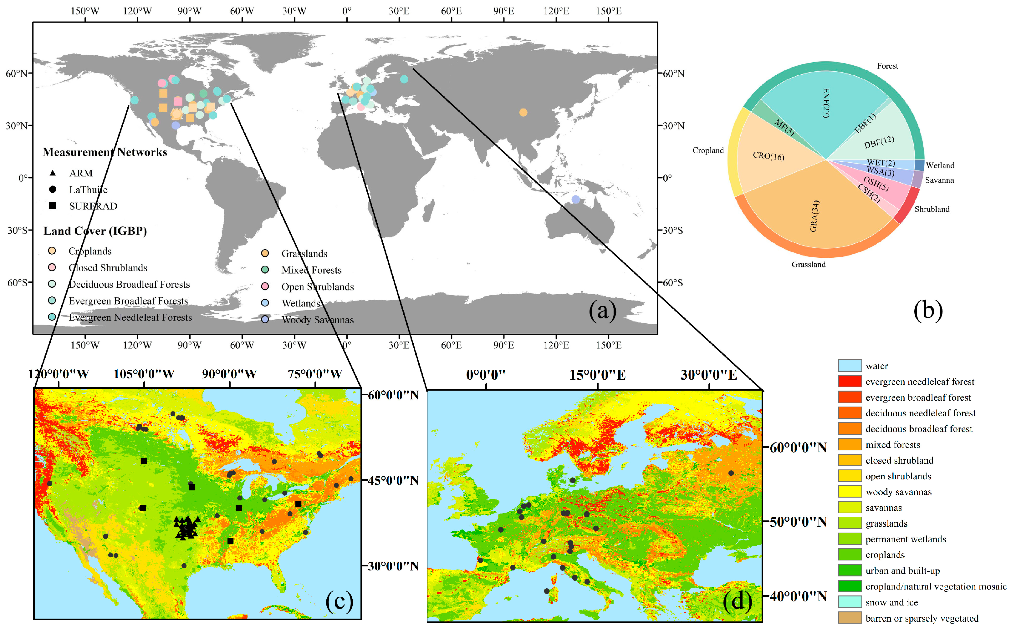
2.1.1. In Situ Measurements
2.1.2. Remotely Sensed Data
- A.
- NDVI from Landsat 5/7/8
- B.
- MODIS data
2.1.3. Clearness Index (CI) Calculation
2.2. Methods
2.2.1. Temporal Expansion Model
- A.
- Sinusoidal model
- B.
- Two existing models (S Model and R Model) and new model
2.2.2. Evaluation Criteria
3. Results
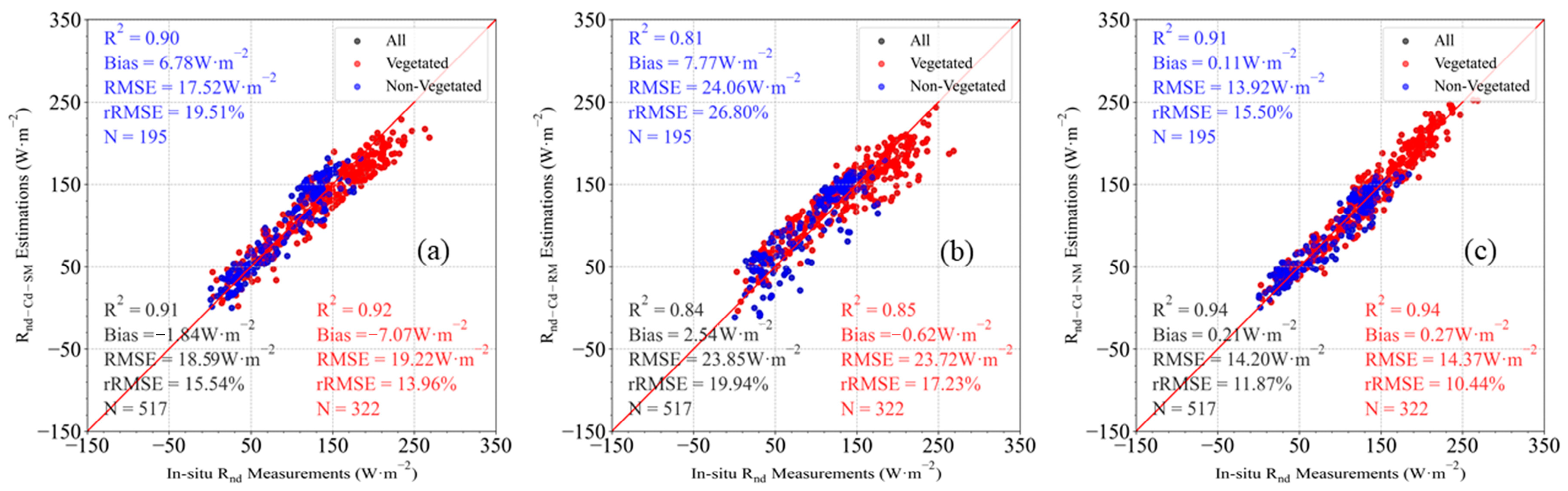
3.1. Evaluation on the Three Cd Models
3.1.1. Validation Accuracy at Site Scale
- A.
- S Model
- B.
- R model
- C.
- New Model
3.1.2. Models Inter-Comparison
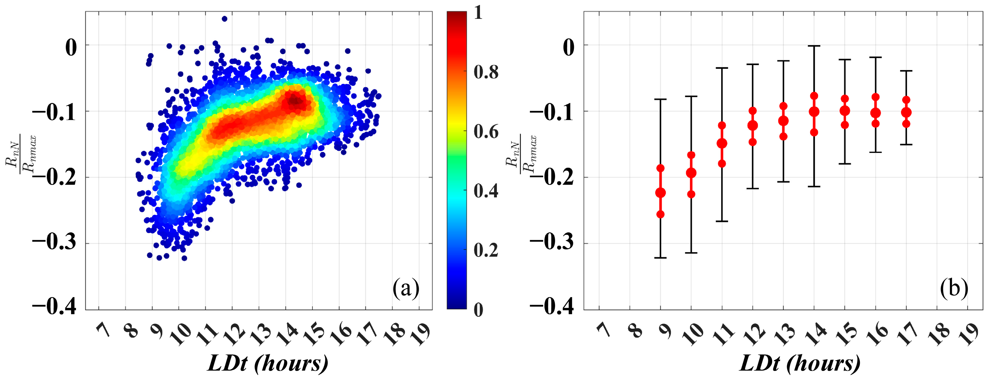
3.2. Further Analysis of New Model
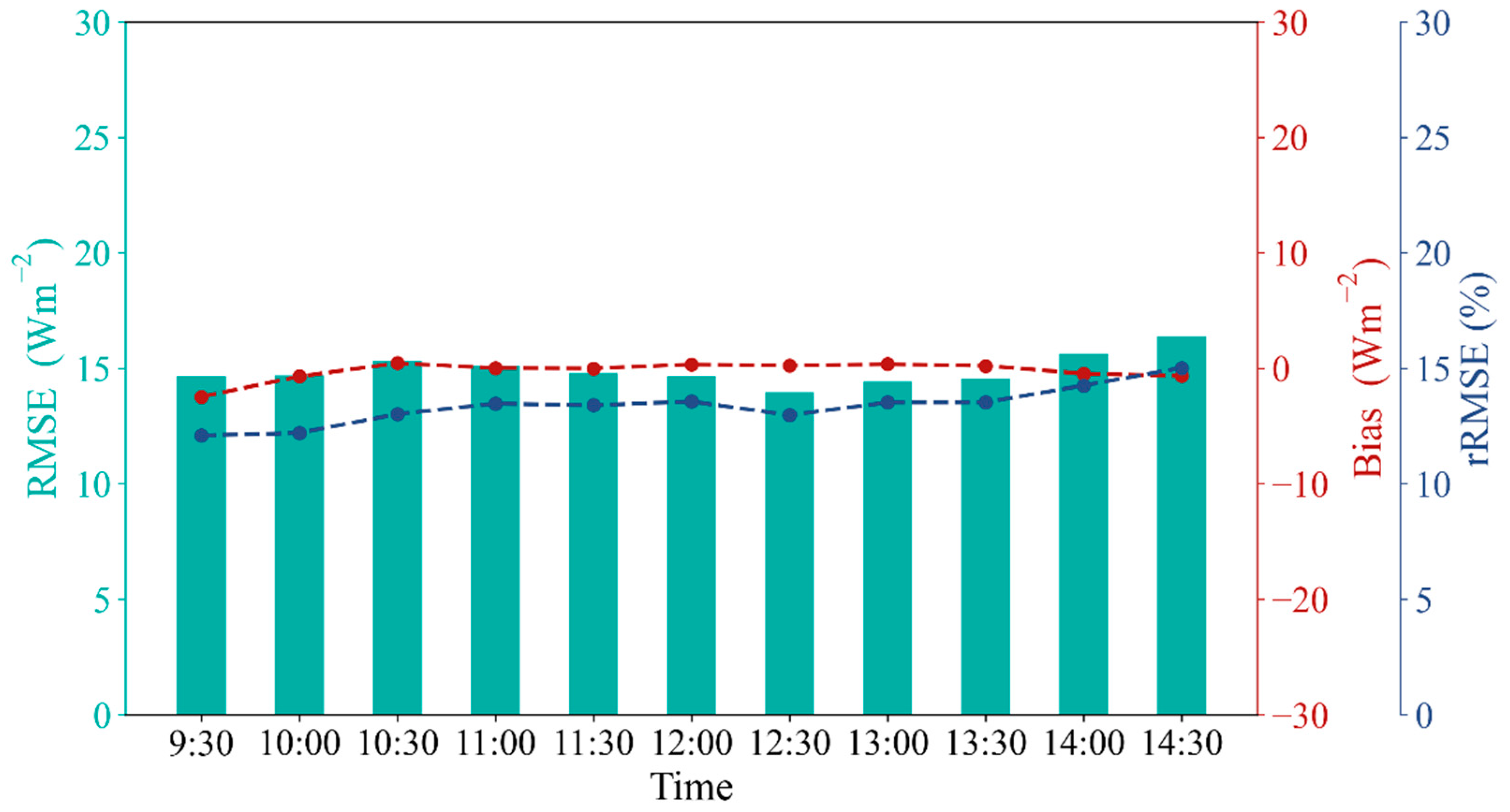
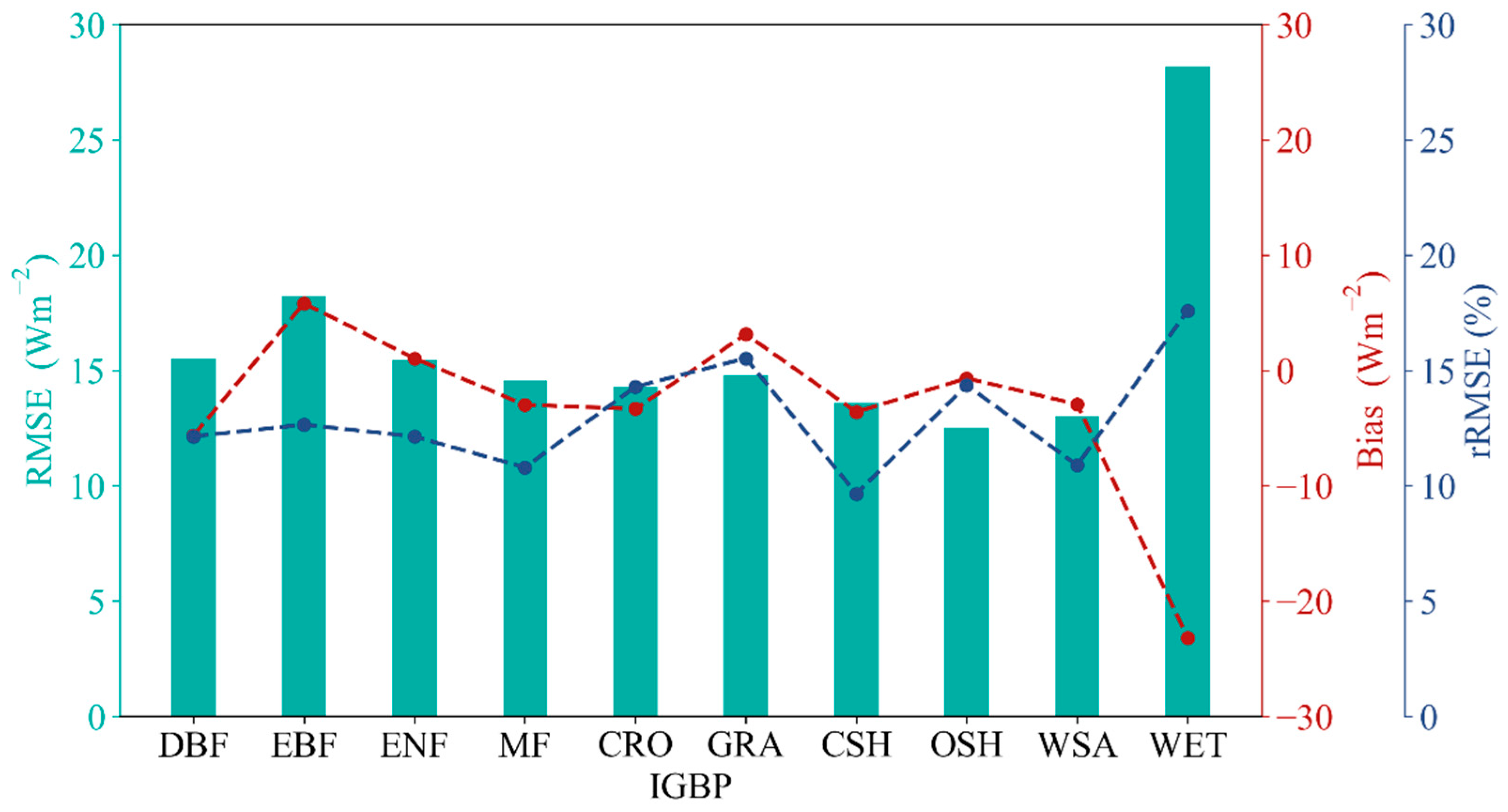
3.2.1. Model Performance Under Different Conditions
3.2.2. Application with the MODIS Data to Estimate Rnd
4. Conclusions
Author Contributions
Funding
Data Availability Statement
Acknowledgments
Conflicts of Interest
References
- Ramírez-Cuesta, J.M.; Vanella, D.; Consoli, S.; Motisi, A.; Minacapilli, M. A satellite stand-alone procedure for deriving net radiation by using SEVIRI and MODIS products. Int. J. Appl. Earth Obs. Geoinf. 2018, 73, 786–799. [Google Scholar]
- Verma, M.; Fisher, J.B.; Mallick, K.; Ryu, Y.; Kobayashi, H.; Guillaume, A.; Moore, G.; Ramakrishnan, L.; Hendrix, V.; Wolf, S.; et al. Global Surface Net-Radiation at 5 km from MODIS Terra. Remote Sens. 2016, 8, 739. [Google Scholar]
- Wu, B.; Liu, S.; Zhu, W.; Yan, N.; Xing, Q.; Tan, S. An Improved Approach for Estimating Daily Net Radiation over the Heihe River Basin. Sensors 2017, 17, 86. [Google Scholar] [CrossRef]
- Li, M.; Zhao, W.; Yang, Y.; Wu, T.; Luo, J. A Solar Radiation-Based Method for Generating Spatially Seamless and Temporally Consistent Land Surface Temperature. IEEE Trans. Geosci. Remote Sens. 2024, 62, 1–15. [Google Scholar]
- Liang, H.; Jiang, B.; Liang, S.; Peng, J.; Li, S.; Han, J.; Yin, X.; Cheng, J.; Jia, K.; Liu, Q.; et al. A global long-term ocean surface daily/0.05 net radiation product from 1983–2020. Sci. Data 2022, 9, 337. [Google Scholar]
- Liang, S.; Wang, K.; Zhang, X.; Wild, M. Review on Estimation of Land Surface Radiation and Energy Budgets From Ground Measurement, Remote Sensing and Model Simulations. IEEE J. Sel. Top. Appl. Earth Obs. Remote Sens. 2010, 3, 225–240. [Google Scholar]
- Shi, C.; Letu, H.; Nakajima, T.Y.; Nakajima, T.; Wei, L.; Xu, R.; Lu, F.; Riedi, J.; Ichii, K.; Zeng, J.; et al. Using midday surface temperature to estimate daily evaporation from of Surface Solar Radiation through the Construction of a Geostationary Satellite Network Observation System. Innovation 2025, 6, 100876. [Google Scholar] [PubMed]
- Yin, X.; Jiang, B.; Liang, S.; Li, S.; Zhao, X.; Wang, Q.; Xu, J.; Han, J.; Liang, H.; Zhang, X.; et al. Significant discrepancies of land surface daily net radiation among ten remotely sensed and reanalysis products. Int. J. Digit. Earth 2023, 16, 3725–3752. [Google Scholar]
- Chen, J.; He, T.; Jiang, B.; Liang, S. Estimation of all-sky all-wave daily net radiation at high latitudes from MODIS data. Remote Sens. Environ. 2020, 245, 111842. [Google Scholar]
- Jiang, B.; Liang, S.; Jia, A.; Xu, J.; Zhang, X.; Xiao, Z.; Zhao, X.; Jia, K.; Yao, Y. Validation of the Surface Daytime Net Radiation Product From Version 4.0 GLASS Product Suite. IEEE Geosci. Remote Sens. Lett. 2019, 16, 509–513. [Google Scholar]
- Li, S.; Jiang, B.; Peng, J.; Liang, H.; Han, J.; Yao, Y.; Zhang, X.; Cheng, J.; Zhao, X.; Liu, Q.; et al. Estimation of the All-Wave All-Sky Land Surface Daily Net Radiation at Mid-Low Latitudes from MODIS Data Based on ERA5 Constraints. Remote Sens. 2021, 14, 33. [Google Scholar]
- Xu, J.; Jiang, B.; Liang, S.; Li, X.; Wang, Y.; Peng, J.; Chen, H.; Liang, H.; Li, S. Generating a High-Resolution Time-Series Ocean Surface Net Radiation Product by Downscaling J-OFURO3. IEEE Trans. Geosci. Remote Sens. 2021, 59, 2794–2809. [Google Scholar]
- Jiang, B.; Han, J.; Liang, H.; Liang, S.; Yin, X.; Peng, J.; He, T.; Ma, Y. The Hi-GLASS all-wave daily net radiation product: Algorithm and product validation. Sci. Remote Sens. 2023, 7, 100080. [Google Scholar]
- Bisht, G.; Venturini, V.; Islam, S.; Jiang, L. Estimation of the net radiation using MODIS (Moderate Resolution Imaging Spectroradiometer) data for clear sky days. Remote Sens. Environ. 2005, 97, 52–67. [Google Scholar]
- Xu, J.; Liang, S.; Jiang, B. A global long-term (1981–2019) daily land surface radiation budget product from AVHRR satellite data using a residual convolutional neural network. Earth Syst. Sci. Data 2022, 14, 2315–2341. [Google Scholar]
- Seguin, B.; Itier, B. Using midday surface temperature to estimate daily evaporation from satellite thermal IR data. Int. J. Remote Sens. 1983, 4, 371–383. [Google Scholar]
- Sobrino, J.A.; Gómez, M.; Jiménez-Muñoz, J.C.; Olioso, A. Application of a simple algorithm to estimate daily evapotranspiration from NOAA–AVHRR images for the Iberian Peninsula. Remote Sens. Environ. 2007, 110, 139–148. [Google Scholar]
- Wassenaar, T.; Olioso, A.; Hasager, C.; Jacob, F.; Chehbouni, A. Estiamation of Evapotranspriation on Heterogeneous Pixels. In Proceedings of the First International Symposium on Recent Advances in Quantitative Remote Sensing, Torrent, Spain, 16–20 September 2002; pp. 458–465. [Google Scholar]
- Rivas, R.E.; Carmona, F. Evapotranspiration in the Pampean Region using field measurements and satellite data. Phys. Chem. Earth Parts A/B/C 2013, 55, 27–34. [Google Scholar]
- Carmona, F.; Rivas, R.; Caselles, V. Development of a general model to estimate the instantaneous, daily, and daytime net radiation with satellite data on clear-sky days. Remote Sens. Environ. 2015, 171, 1–13. [Google Scholar]
- Phillips, T.J.; Klein, S.A.; Ma, H.Y.; Tang, Q.; Xie, S.; Williams, I.N.; Santanello, J.A.; Cook, D.R.; Torn, M.S. Using ARM Observations to Evaluate Climate Model Simulations of Land-Atmosphere Coupling on the U.S. Southern Great Plains. J. Geophys. Res. Atmos. 2017, 122, 11–524. [Google Scholar]
- Augustine, J.A.; DeLuisi, J.J.; Long, C.N. SURFRAD-A National Surface Radiation Budget Network for Atmospheric Research. Bull. Am. Meteorol. Soc. 2000, 81, 18. [Google Scholar]
- Loveland, T.R.; Belward, A.S. The IGBP-DIS global 1km land cover data set, DISCover: First results. Int. J. Remote Sens. 1997, 18, 3289–3295. [Google Scholar]
- Wang, Y.; Jiang, B.; Liang, S.; Wang, D.; He, T.; Wang, Q.; Zhao, X.; Xu, J. Surface Shortwave Net Radiation Estimation from Landsat TM/ETM+ Data Using Four Machine Learning Algorithms. Remote Sens. 2019, 11, 2847. [Google Scholar]
- Roy, D.P.; Kovalskyy, V.; Zhang, H.K.; Vermote, E.F.; Yan, L.; Kumar, S.S.; Egorov, A. Characterization of Landsat-7 to Landsat-8 reflective wavelength and normalized difference vegetation index continuity. Remote Sens. Environ. 2016, 185, 57–70. [Google Scholar]
- Masek, J.G.; Vermote, E.F.; Saleous, N.E.; Wolfe, R.; Hall, F.G.; Huemmrich, K.F.; Gao, F.; Kutler, J.; Lim, T.K. A Landsat Surface Reflectance Dataset for North America, 1990–2000. IEEE Geosci. Remote Sens. Lett. 2006, 3, 68–72. [Google Scholar]
- Iziomon, M.G.; Mayer, H.; Matzarakis, A. Empirical Models for Estimating Net Radiative Flux: A Case Study for Three Mid-Latitude Sites with Orographic Variability. Astrophys. Space Sci. 2000, 273, 18. [Google Scholar]
- Crawford, T.M.; Duchon, C.E. An Improved Parameterization for Estimating Effective Atmospheric Emissivity for Use in Calculating Daytime Downwelling Longwave Radiation. J. Appl. Meteorol. Climatol. 1999, 38, 7. [Google Scholar]
- Jiang, B.; Zhang, Y.; Liang, S.; Wohlfahrt, G.; Arain, A.; Cescatti, A.; Georgiadis, T.; Jia, K.; Kiely, G.; Lund, M.; et al. Empirical estimation of daytime net radiation from shortwave radiation and ancillary information. Agric. For. Meteorol. 2015, 211, 23–36. [Google Scholar]


| Abbr. | Number of Sites | Time Period | Temporal Resolution | Reference |
|---|---|---|---|---|
| ARM | 29 | 1994~2017 | 1 min | [21] |
| La Thuile | 70 | 1996~2015 | 30 min | [8] |
| SURFRAD | 6 | 1995~2017 | 1 or 3 min | [22] |
| MODIS Product | Spatial Resolution | Parameters Used |
|---|---|---|
| MOD/MYD02 | 1 km | 1 km_RefSB, 1 km_Emissive |
| MOD/MYD03 | 1 km | SolarZenith (SZA), SolarAzimuth (SAA), SensorZenith (VZA), SensorAzimuth (VAA), Height |
| MOD/MYD35 | 1 km | Cloud Mask |
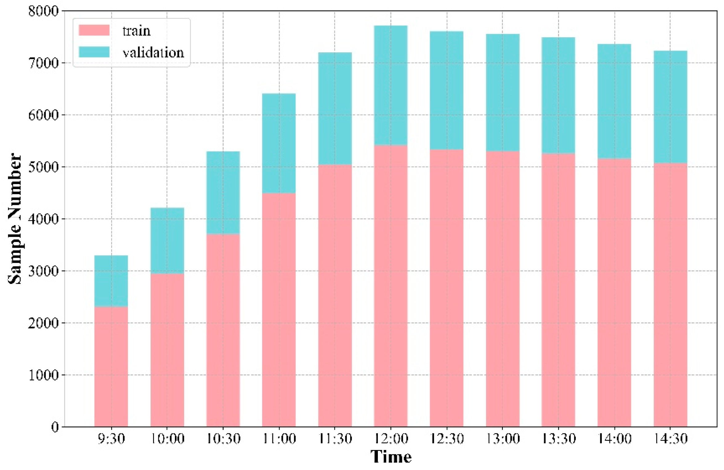
| Training | Validation | |||
|---|---|---|---|---|
| Cd | Rni | Rnd * | ||
| Time | No. of Samples | No. of Samples | No. of Samples | |
| S Model | 12:00 | 5393 | 2315 | 4992 |
| 13:00 | 5288 | 2267 | ||
| 14:00 | 5147 | 2206 | ||
| R Model | 10:00~11:00 | 7730 | 3314 | 3314 |
| New Model | 9:30~12:30 (30 min an interval) | |||
| Vegetated | 31,450 | 13,624 | 4668 | |
| Non-vegetated | 18,431 | 7759 | 2730 | |
| Common validation samples: No. = 517 | ||||
| Time | Original Coefficient | Calibrated Coefficient | ||||
|---|---|---|---|---|---|---|
| 12:00 | 0.0026 | 0.0756 | 0.0026 | 0.0383 | ||
| 13:00 | 0.0028 | 0.0820 | 0.0026 | 0.0375 | ||
| 14:00 | 0.0027 | 0.1240 | 0.0027 | 0.0467 | ||
| Original Coefficient | Corrected Coefficient | ||
|---|---|---|---|
| 0.43 | 54 | 0.3819 | 68.27 |
| Condition | ||||||
|---|---|---|---|---|---|---|
| NDVI ≥ 0.1 | 0.9204 | −0.0052 | 0.0280 | −0.0039 | 0.1146 | −0.9468 |
| NDVI < 0.1 | 0.9041 | −0.0070 | 0.0519 | −0.0036 | 0.0939 | −0.7710 |
Disclaimer/Publisher’s Note: The statements, opinions and data contained in all publications are solely those of the individual author(s) and contributor(s) and not of MDPI and/or the editor(s). MDPI and/or the editor(s) disclaim responsibility for any injury to people or property resulting from any ideas, methods, instructions or products referred to in the content. |
© 2025 by the authors. Licensee MDPI, Basel, Switzerland. This article is an open access article distributed under the terms and conditions of the Creative Commons Attribution (CC BY) license (https://creativecommons.org/licenses/by/4.0/).
Share and Cite
Han, J.; Jiang, B.; Zhao, Y.; Peng, J.; Li, S.; Liang, H.; Yin, X.; Chen, Y. A General Model for Converting All-Wave Net Radiation at Instantaneous to Daily Scales Under Clear Sky. Remote Sens. 2025, 17, 2364. https://doi.org/10.3390/rs17142364
Han J, Jiang B, Zhao Y, Peng J, Li S, Liang H, Yin X, Chen Y. A General Model for Converting All-Wave Net Radiation at Instantaneous to Daily Scales Under Clear Sky. Remote Sensing. 2025; 17(14):2364. https://doi.org/10.3390/rs17142364
Chicago/Turabian StyleHan, Jiakun, Bo Jiang, Yu Zhao, Jianghai Peng, Shaopeng Li, Hui Liang, Xiuwan Yin, and Yingping Chen. 2025. "A General Model for Converting All-Wave Net Radiation at Instantaneous to Daily Scales Under Clear Sky" Remote Sensing 17, no. 14: 2364. https://doi.org/10.3390/rs17142364
APA StyleHan, J., Jiang, B., Zhao, Y., Peng, J., Li, S., Liang, H., Yin, X., & Chen, Y. (2025). A General Model for Converting All-Wave Net Radiation at Instantaneous to Daily Scales Under Clear Sky. Remote Sensing, 17(14), 2364. https://doi.org/10.3390/rs17142364