HyperTransXNet: Learning Both Global and Local Dynamics with a Dual Dynamic Token Mixer for Hyperspectral Image Classification

Abstract

Recent advances in hyperspectral image (HSI) classification have demonstrated the effectiveness of hybrid architectures that integrate convolutional neural networks (CNNs) and Transformers, leveraging CNNs for local feature extraction and Transformers for global dependency modeling. However, existing fusion approaches face three critical challenges: (1) insufficient synergy between spectral and spatial feature learning due to rigid coupling mechanisms; (2) high computational complexity resulting from redundant attention calculations; and (3) limited adaptability to spectral redundancy and noise in small-sample scenarios. To address these limitations, we propose HyperTransXNet, a novel CNN-Transformer hybrid architecture that incorporates adaptive spectral-spatial fusion. Specifically, the proposed HyperTransXNet comprises three key modules: (1) a Hybrid Spatial-Spectral Module (HSSM) that captures the refined local spectral-spatial features and models global spectral correlations by combining depth-wise dynamic convolution with frequency-domain attention; (2) a Mixture-of-Experts Routing (MoE-R) module that adaptively fuses multi-scale features by dynamically selecting optimal experts via Top-K sparse weights; and (3) a Spatial-Spectral Tokens Enhancer (SSTE) module that ensures causality-preserving interactions between spectral bands and spatial contexts. Extensive experiments on the Indian Pines, Houston 2013, and WHU-Hi-LongKou datasets demonstrate the superiority of HyperTransXNet.

1. Introduction

Hyperspectral images (HSIs), characterized by their contiguous spectral bands that span the electromagnetic spectrum, offer a distinctive three-dimensional spatial-spectral representation of surface materials. This dense spectral sampling enables the precise discrimination of land cover types, rendering HSIs indispensable in applications such as environmental monitoring [1], precision agriculture, and urban planning [2]. Nevertheless, the high dimensionality of HSIs introduces inherent challenges, including spectral redundancy, spatial heterogeneity, and the curse of dimensionality, all of which complicate feature extraction and classification. Traditional machine learning methods, such as support vector machines (SVMs) and random forests, often struggle with these complexities due to their dependence on handcrafted features and their limited capacity to model nonlinear spectral-spatial relationships.

Recent advances in deep learning have transformed hyperspectral imaging (HSI) classification by automating feature extraction [3,4]. Early studies primarily employed two-dimensional convolutional neural networks (2D-CNNs) to capture spatial patterns by sliding fixed kernels across hyperspectral image (HSI) patches. For example, Paoletti et al. [5] proposed a 2D-CNN with shortcut connections. Although such architectures are proficient at extracting local textures and edges, they inherently disregard the rich spectral correlations present across hundreds of contiguous bands. To address this limitation, three-dimensional convolutional neural networks (3D-CNNs) emerged as a transformative approach by explicitly modeling spectral-spatial cubes via volumetric convolutions. A notable instance is HybridSN [6], which hierarchically integrates 3D convolutions for joint spectral-spatial encoding with 2D convolutions for spatial refinement. This hybrid architecture significantly enhances classification accuracy by leveraging inter-band dependencies. However, 3D-CNNs are challenged by prohibitive computational costs and parameter redundancy, especially in scenarios with limited labeled data.

Although 2D- and 3D-CNNs have laid a robust foundation for automated feature learning, they are subject to two main limitations. First, there is a spatial-spectral decoupling issue: 2D-CNNs prioritize spatial details at the expense of spectral coherence, while 3D-CNNs encounter challenges in balancing computational efficiency with spectral fidelity. Second, both architectures inadequately capture global dependencies; their localized receptive fields hinder the modeling of long-range contextual relationships, which can lead to misclassifications in heterogeneous or fragmented regions. These constraints underscore the necessity for novel architectures that seamlessly integrate spectral-spatial dynamics while maintaining computational efficiency—a gap that subsequent advancements in attention mechanisms and hybrid frameworks seek to address.

The emergence of Vision Transformers (ViTs) has introduced a paradigm shift in hyperspectral image (HSI) classification by leveraging self-attention mechanisms to capture global spectral-spatial dependencies. In contrast to convolutional neural networks (CNNs), which are limited to localized convolutions, ViTs represent HSIs as sequences of tokens, thereby enabling the modeling of long-range interactions. For example, the Spectral-Spatial Feature Tokenization Transformer (SSFTT) [7] pioneers a hierarchical framework in which preliminary spectral-spatial features are extracted using shallow CNN layers, tokenized, and subsequently processed by Transformer blocks to capture global contextual relationships. This hybrid design harmonizes the preservation of local details with the attainment of global coherence, achieving state-of-the-art accuracy on datasets such as Indian Pines. Despite these advancements, Transformer-based methods are hindered by two primary limitations: (1) quadratic complexity, whereby self-attention scales quadratically with sequence length, making it computationally prohibitive for high-resolution HSIs; and (2) spatial discontinuity, as fixed-size patch tokenization disrupts the inherent spatial continuity of HSIs, thereby generating artifacts in fine-grained classification maps, particularly for small or irregular targets.

To mitigate these issues, Mamba-based architectures have emerged as lightweight alternatives. By combining the computational efficiency of convolutions with selective state transitions, Mamba models achieve linear computational scaling while preserving global sequence modeling capabilities. For instance, SpectralMamba [8] introduces a dynamic spectral masking mechanism and a bidirectional scanning strategy that adaptively groups redundant bands and propagates contextual dependencies across the spectral dimension. Similarly, DualMamba [9] presents a dual-path architecture incorporating parallel spatial and spectral SSM blocks, which simultaneously model local spatial details and global spectral trends. However, Mamba-based methods are still constrained by their implicit feature fusion mechanisms; for example, SpectralMamba relies on post-hoc concatenation of spectral and spatial features and lacks dynamic interaction modules capable of suppressing noise or enhancing discriminative bands.

Despite recent advancements, several critical challenges remain unresolved.

• Current fusion methodologies exhibit insufficient spectral-spatial synergy; they tend to integrate local and global features in a rigid manner, thereby failing to adaptively balance their respective contributions.
• Computational inefficiencies persist, as redundant attention calculations and suboptimal parameterizations impede real-time deployment.
• Conventional architectures demonstrate a pronounced sensitivity to spectral noise, struggling to suppress redundant bands and enhance discriminative features, particularly under conditions of significant noise or limited sample sizes.

These limitations present critical challenges for hyperspectral image classification, particularly in effectively leveraging high-dimensional spectral features and modeling spatial-spectral relationships. To address these challenges, we propose HyperTransXNet, a novel CNN-Transformer hybrid architecture that integrates spectral and spatial dynamics through three meticulously designed modules. First, the Hybrid Spatial-Spectral Module (HSSM) combines depth-wise dynamic convolutions with frequency-domain attention to simultaneously refine local details and global spectral correlations. Second, the Mixture-of-Experts Routing (MoE-R) module utilizes a dynamic gating mechanism to select optimal multi-scale features via Top-K sparse activation. Third, the Spatial-Spectral Tokens Enhancer (SSTE) module bolsters robustness by preserving causality-aware interactions among tokens, aligning spectral and spatial features with $1\times 1$ convolutions, and further refining them through MoE-R, thereby effectively suppressing noise while maintaining structural coherence. The main contributions of this paper are as follows:

• We introduce HyperTransXNet, a novel hybrid framework that integrates CNN-driven local feature extraction, Transformer-based global dependency modeling, and Mamba-inspired efficiency through dynamic spectral-spatial fusion, thereby addressing the limitations of isolated architectural paradigms.
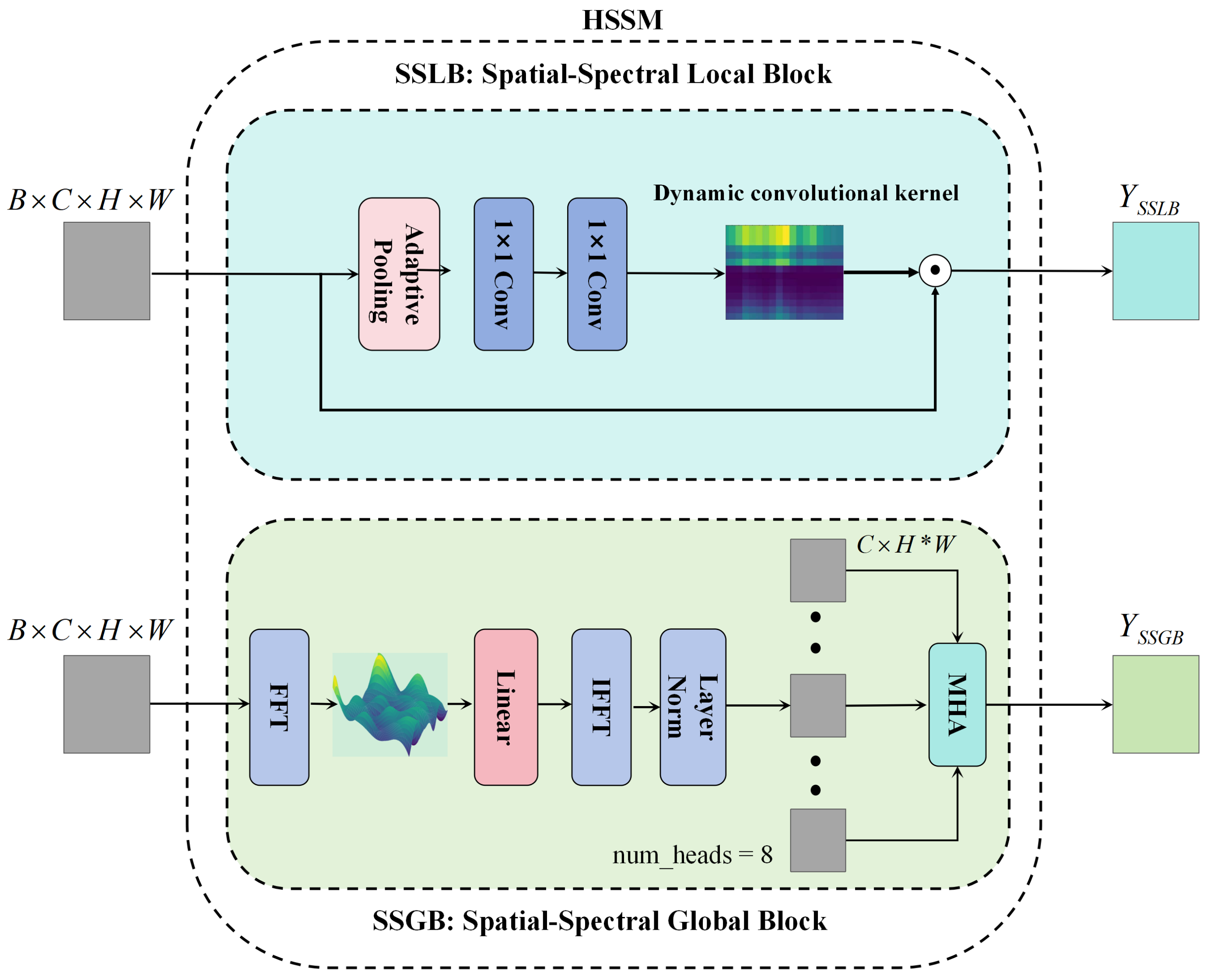
• We propose a Hybrid Spatial-Spectral Module (HSSM) that integrates depth-wise dynamic convolutions with frequency-domain attention. This design facilitates the simultaneous enhancement of local textures and global spectral correlations without incurring additional computational overhead.
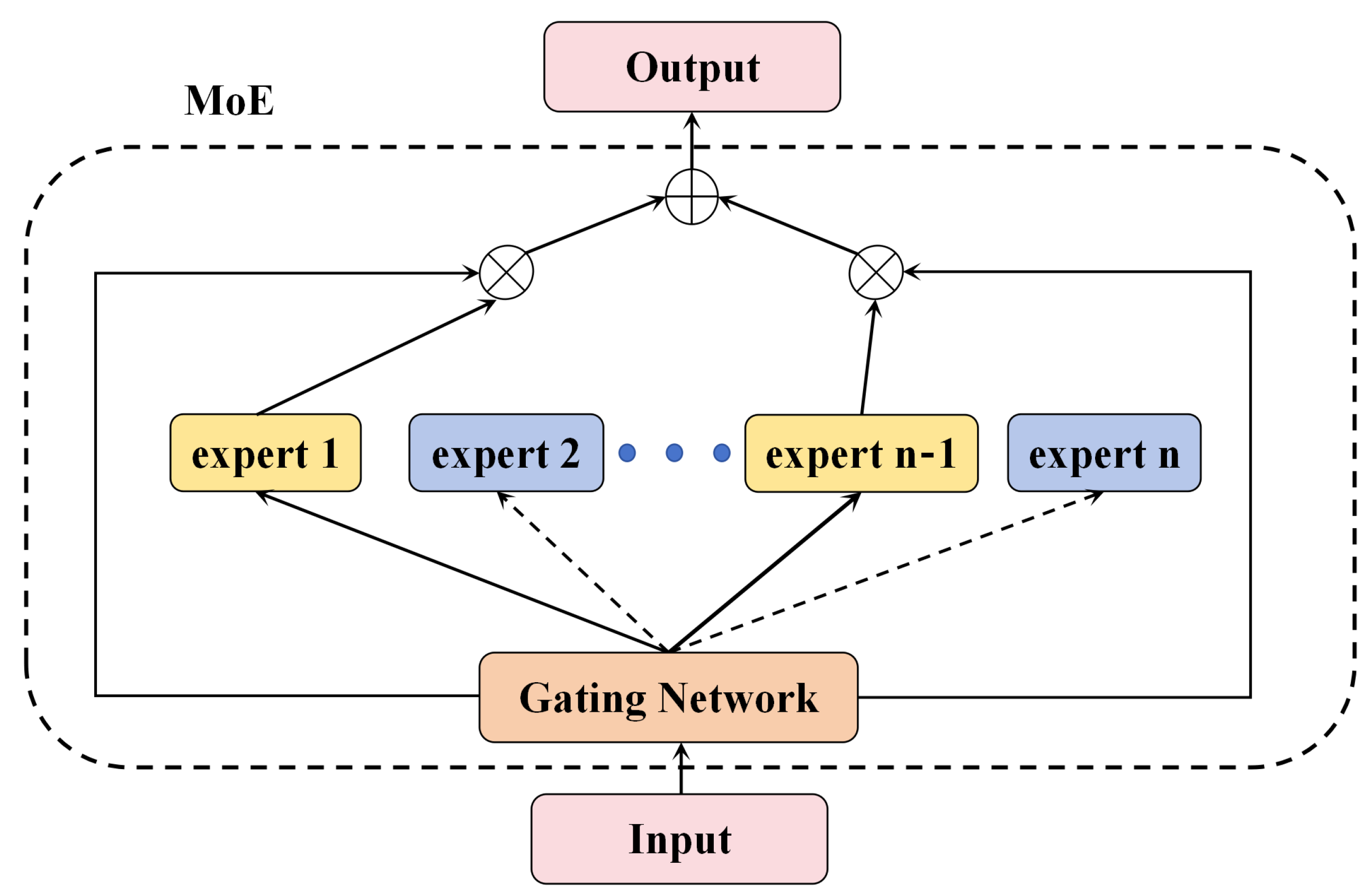
• We employ the Top-K sparse Mixture-of-Experts routing mechanism, marking its inaugural application in hyperspectral classification, which achieves parameter-efficient multi-scale feature aggregation via context-aware expert selection.
• Extensive experiments conducted on three public HSI datasets demonstrate that the proposed HyperTransXNet outperforms state-of-the-art methods based on CNNs and Transformers.

The remainder of this paper is organized as follows. Section 2 reviews the literature on image classification methods based on convolutional neural networks (CNNs), Transformer architectures, and studies on Mixture-of-Experts (MoE) routing methods. Section 4 details the proposed approach and its constituent components. Section 5 introduces several benchmark high-resolution hyperspectral image (HSI) datasets, describes the experimental settings, and presents the results along with a thorough analysis. Finally, Section 6 concludes the paper.

2. Related Works

Hyperspectral image (HSI) classification methodologies have advanced through three distinct research paradigms: convolutional neural networks (CNNs)-based, Transformers-based, and Mamba-based approaches. Each paradigm targets specific facets of spectral-spatial feature learning while simultaneously addressing the intrinsic limitations associated with the individual methodologies.

2.1. CNN-Based Hyperspectral Image Classification

With the rise of deep learning, CNN-based hyperspectral image (HSI) classification methods have also received extensive research attention [3,10,11,12,13,14,15,16,17,18,19,20]. For example, Paoletti et al. [5] proposed a 2D-CNN model for HSI classification, introducing shortcut connections to allow low-level features to directly pass to subsequent layers, thereby enhancing feature expression capabilities. However, 2D-CNNs inherently neglect spectral correlations across hundreds of contiguous bands, limiting their discriminative power for materials with subtle spectral variations (e.g., vegetation subtypes).

To address this limitation, 3D convolutional neural networks (3D-CNNs) have been developed to explicitly model spectral-spatial cubes using volumetric convolutions. For example, Roy et al. [6] introduced a hybrid 3D-2D CNN model (HybridSN) that hierarchically combines 3D convolutions for joint spectral-spatial encoding with 2D convolutions for spatial refinement, achieving a 12% improvement in classification accuracy over conventional 2D-CNNs on the Indian Pines dataset. Similarly, Mei et al. [21] proposed an approach that integrates attention mechanisms with bidirectional long short-term memory (BiLSTM) networks within a CNN framework. Nonetheless, despite the superior local feature extraction capabilities of CNNs, they exhibit notable limitations in representing global features and capturing long-range dependencies in HSI data. Moreover, 3D-CNNs confront two critical challenges: (1) fixed receptive fields limit adaptability to varying spectral curve complexities, and (2) quadratic growth in the number of parameters increases the risk of overfitting, particularly in small-sample scenarios.

2.2. Transformers-Based Hyperspectral Image Classification

To address the limitations of traditional CNNs, some researchers have introduced Transformer to solve the problem of HSI classification [22,23,24,25,26,27,28,29]. For example, Vision Transformers (ViTs) [30] have redefined hyperspectral image (HSI) classification by leveraging self-attention mechanisms to model global spectral-spatial dependencies, thereby overcoming the localized receptive field limitations inherent in convolutional neural networks (CNNs). In contrast to traditional CNNs, ViTs conceptualize HSIs as sequences of tokens, which facilitates interactions between distant pixels and spectral bands. A seminal example of this approach is the Spectral-Spatial Feature Tokenization Transformer (SSFTT) [7], which initially extracts shallow spatial-spectral features using hierarchical 3D-CNN layers and subsequently tokenizes these features into semantic vectors for processing by Transformer blocks. This hybrid architecture achieves an overall accuracy (OA) by effectively integrating local texture details with global spectral trends. Another innovative architecture, MorphFormer [31], integrates morphological convolution operations with spectral-spatial attention mechanisms to enhance structural feature learning. By applying learnable morphological filters (e.g., erosion and dilation) to HSI tokens, MorphFormer captures geometric primitives such as edges and shapes, which are critical for identifying irregular targets like roads and parking lots.

Recent advancements further explore specialized attention mechanisms for HSI. For example, HiT [32] embeds 3D convolutions within Transformer blocks to propagate local spectral context. Despite their success, Transformer-based methods face two fundamental challenges: (1) Quadratic Computational Complexity: self-attention scales quadratically with the number of tokens, rendering them inefficient for high-resolution HSIs. (2) Spatial discontinuity: fixed-size patch tokenization disrupts the inherent spatial continuity of HSIs, leading to misclassification at patch boundaries. To mitigate these limitations, recent works such as Swin-HSI [33] employ shifted window attention to reduce computational costs. However, these adaptations often sacrifice global context modeling for efficiency, underscoring the need for architectures that balance computational tractability with comprehensive spectral-spatial reasoning—a goal central to our proposed HyperTransXNet.

2.3. Mamba-Based Hyperspectral Image Classification

Recent advancements in state space models (SSMs) have driven the development of Mamba-based architectures, which integrate the computational efficiency of convolutional operations with the extensive sequence modeling capabilities of Transformers. By employing selective state transitions and linear-time scanning mechanisms, Mamba models offer enhanced scalability for high-dimensional hyperspectral data while ensuring minimal computational overhead [8,34,35].

For example, SpectralMamba [8] represents a pioneering contribution by introducing a dynamic spectral masking mechanism that adaptively clusters redundant spectral bands. Additionally, it employs bidirectional spectral scanning, processing spectral sequences in both forward and backward directions, to effectively model long-range dependencies across bands. Building on this concept, DualMamba [9] proposes a dual-path architecture featuring parallel spatial and spectral SSM blocks. In this framework, the spatial branch applies a 2D-SSM to capture local textures, whereas the spectral branch utilizes a 1D-SSM to model inter-band correlations, resulting in an overall accuracy of 98.74% on the WHU-Hi-LongKou dataset through disentangled yet complementary feature learning. Moreover, emerging variants such as HyperMamba [36] further enhance the applicability of the Mamba paradigm by integrating 3D spectral-spatial SSM blocks; HyperMamba processes hyperspectral image (HSI) cubes as continuous three-dimensional sequences and dynamically adjusts state transitions based on spectral gradients.

Despite significant advancements in hyperspectral image (HSI) classification, three fundamental limitations persist across current paradigms:

• Ineffective joint spectral-spatial representation learning: CNN-based methods are constrained by fixed receptive fields that fail to adapt to the varying complexities of spectral curves. In contrast, Mamba architectures suffer from fragmented local context modeling due to their unidirectional scanning. Although Transformer-based approaches effectively model global dependencies, they incur quadratic computational costs, thereby limiting their applicability to large-scale HSIs.
• Suboptimal feature fusion strategies: Contemporary methods predominantly rely on static fusion techniques to integrate spectral and spatial features. These heuristic approaches lack the adaptability needed to suppress noisy bands or to emphasize discriminative spectral regions, resulting in performance degradation in complex scenes, such as those encountered in urban-rural transitions.

In this paper, we propose HyperTransXNet, a unified architecture that redefines spectral-spatial fusion through three key modules: (1) The Hybrid Spatial-Spectral Module (HSSM) integrates depth-wise dynamic convolutions, with kernel parameters adaptively generated from the global context and frequency domain attention to jointly refine local textures and global spectral trends. This approach effectively eliminates the spatial-spectral decoupling commonly observed in conventional CNNs and Mamba models. (2) Mixture-of-Experts Routing (MoE-R) utilizes Top-K sparse gating to dynamically select optimal experts for feature aggregation. (3) By integrating lightweight dynamic operations with frequency-domain regularization, HyperTransXNet significantly reduces parameter redundancy.

2.4. Different from TransXNet

There are three main differences between TransXNet [37] and our proposed HyperTransXNet. The first difference lies in the feature extraction method. TransXNet utilizes deep convolution and global attention modules to extract local features and global representations, respectively. In contrast, HyperTransXNet employs two different modules: the Spatial-Spectral Local Block (SSLB) and the Spatial-Spectral Global Block (SSGB). SSLB achieves local feature extraction through adaptively generated convolution kernels, while SSGB combines frequency domain attention and multi-head attention mechanisms to capture global representations. The second difference is in the application of the methods. TransXNet is primarily applied in general computer vision fields, whereas our proposed HyperTransXNet focuses on hyperspectral image classification. The third difference is in the feature fusion mechanism. TransXNet mainly uses an improved multi-scale feedforward network for feature fusion, while HyperTransXNet introduces a Spatial-Spectral Tag Enhancer (SSTE) to merge local and global features. In SSTE, we introduce a Mixture-of-Experts routing mechanism (MoE-R) that selectively activates suitable experts through a Top-K sparse gating strategy and constructs a selection matrix, ultimately merging the outputs of both to achieve feature aggregation.

3. MoE

The Mixture-of-Experts (MoE) model is an advanced neural network architecture designed to enhance overall performance by integrating predictions from multiple expert sub-models. Due to its sophistication, this architecture has been widely applied in various fields, including natural language processing [38,39,40,41,42]. The fundamental concept underlying the MoE model involves partitioning the input data among specialized sub-models, each proficient in handling specific tasks and subsequently aggregating their outputs to generate a final prediction. This allocation mechanism is typically dynamic, adjusting based on the characteristics of the input data to ensure that each expert focuses on the data type or task for which it is best suited, thereby achieving efficient and accurate predictions. As shown in Figure 1.The MoE model consists of two main components: the Gating Network and the experts. The Gating Network dynamically determines which expert sub-model or models should process a given input by analyzing its features and computing the corresponding weights or importance for each expert, subsequently allocating the input based on these weights. The experts comprise multiple independent neural networks, each dedicated to processing a specific subset of the input data or a particular task. Ultimately, the MoE model consolidates the prediction results from multiple experts, leveraging the unique strengths of each to improve overall performance. The formulation of the MoE model is expressed as follows:   

$$\begin{array}{cc}\hfill & {\mathbf{g}}_i\left(x\right)=\mathrm{softmax}\left({\mathbf{W}}_g·x\right)\hfill \\ \hfill & {\mathbf{E}}_i\left(x\right)=f_{\mathrm{expert}}^i(x;{\theta }_i)\hfill \\ \hfill & \mathbf{output}=\sum _{i=1}^N{\mathbf{g}}_i\left(x\right)·{\mathbf{E}}_i\left(x\right)\hfill \end{array}$$

(1)

Here, ${\mathbf{W}}_g$ is the weight matrix of the gated network, N is the number of experts, ${\theta }_i$ is the parameter of the $i-th$ expert, and $f_{\mathrm{expert}}^i$ can be any neural network (such as fully connected layers, Transformers, etc.). According to the formula, the gated network calculates the weights of each expert for the input sample x and generates a probability distribution ${\mathbf{g}}_i\left(x\right)$. The ${\mathbf{E}}_i\left(x\right)$ in the experts network corresponds to the output of the i-th expert.

4. Proposed Methodology

4.1. Overview

Figure 2 illustrates the proposed HyperTransXNet architecture, a hierarchical hybrid model that integrates convolutional neural networks and Transformers to harmonize spectral-spatial dynamics through adaptive feature fusion. The architecture comprises three primary components. First, the Stem module performs lightweight spectral-spatial preprocessing for initial feature extraction. Second, the HyperTransXNet Blocks consist of cascaded units that integrate Hybrid Spatial-Spectral Modules (HSSMs) and a Spatial-Spectral Tokens Enhancer (SSTE) to enable joint local and global refinement. Third, the Classification Head dynamically aggregates features and generates predictions through adaptive pooling and fully connected layers.

4.2. Stem

The Stem module performs lightweight spectral-spatial preprocessing to reduce dimensionality while preserving discriminative features. It combines $1\times 1$ convolutional layers for spectral compression and $3\times 3$ convolutions for spatial detail extraction. The Stem can be expressed as follows:

$$\begin{array}{cc}\hfill & \mathbf{Stem}\left(\mathbf{X}\right)={\mathrm{Conv}}_{3\times 3}\left(\mathrm{ReLU}\left({\mathrm{Conv}}_{1\times 1}\left(\mathbf{X}\right)\right)\right)\hfill \end{array}$$

(2)

Here, $\mathbf{X}\in {\mathbb{R}}^{B\times C\times H\times W}$ represents the input feature map.

4.3. HyperTransXNet Block

To enhance the local feature extraction capability of the Transformer model, numerous studies have endeavored to integrate convolution and attention mechanisms. However, these methods rely on fixed-sized convolution kernels, rendering them less adaptable to the significant variations in spectral curves across different land cover categories. To address this challenge, we propose a novel HyperTransXNet Block that dynamically fuses global and local information to precisely enhance the frequency bands critical to classification tasks. As illustrated in Figure 2, the input feature map $\mathbf{X}\in {\mathbb{R}}^{B\times C\times H\times W}$ is initially processed by the Stem module. Thereafter, a branch replication operation generates two identical feature maps, which are respectively forwarded to the Spatial-Spectral Local Block (SSLB) and the Spatial Spectral Global Block (SSGB), resulting in the feature maps ${\mathbf{Y}}_{SSLB}$ and ${\mathbf{Y}}_{SSGB}$. Ultimately, the Spatial Spectral Tokens Enhancer fuses the local features and global representations efficiently to produce the output feature map $\mathbf{Y}\in {\mathbb{R}}^{B\times C\times H\times W}$. Overall, the proposed HyperTransXNet Block can be expressed as follows:

$$\begin{array}{cc}\hfill & {\mathbf{X}}_1,{\mathbf{X}}_2=\mathrm{Copy}\left(\mathrm{Stem}\left(\mathbf{X}\right)\right)\hfill \\ \hfill & {\mathbf{Y}}_{SSLB},{\mathbf{Y}}_{SSGB}=\mathrm{SSLB}\left({\mathbf{X}}_1\right),\mathrm{SSGB}\left({\mathbf{X}}_2\right)\hfill \\ \hfill & \mathbf{Y}=\mathrm{SSTE}({\mathbf{Y}}_{SSLB},{\mathbf{Y}}_{SSGB})\hfill \end{array}$$

(3)

Hybrid Spatial-Spectral Module (HSSM)

Traditional hyperspectral image classification methods often depend excessively on a single algorithm or approach, limiting their ability to fully harness the complementary nature of spectral and spatial features. To overcome this limitation, we propose a novel Hybrid Spatial-Spectral Module (HSSM) that integrates multiple sub-modules designed to capitalize on the strengths of diverse architectural approaches, thereby significantly enhancing classification accuracy. Specifically, the HSSM comprises two complementary sub-modules: the Spatial-Spectral Local Block (SSLB), which efficiently extracts local spectral-spatial features via depth-wise separable convolution, and the Spatial-Spectral Global Block (SSGB), which captures global spectral-spatial representations using multi-head attention mechanisms. This modular design not only enables the synergistic optimization of local and global features but also fully exploits the underlying relationships between spectral and spatial information, resulting in an improved feature representation for hyperspectral image classification.

Spatial-Spectral Local Block(SSLB): The SSLB efficiently extracts local information, utilizing depth-wise separable convolution with adaptively generated kernels. Its core structure comprises three components: a dynamic weight generation network, an input unfolding layer, and the application of the dynamic weights (see Figure 3 and Algorithm 1). Given an input feature ${\mathbf{X}}_1\in {\mathbb{R}}^{B\times C\times H\times W}$, the spatial dimensions are first compressed to $(B,C,1,1)$ via an adaptive average pooling (AAP) layer within the dynamic weight generation network. Subsequently, two consecutive $1\times 1$ convolutions interleaved with GELU activations are employed to generate the dynamic convolution kernel parameters. The first $1\times 1$ convolution maintains channel consistency, while the second increases the number of $1\times 1$ output channels by a factor of $K^2$. The input feature is then padded using reflection padding (with a padding width of $P=K/2$) to preserve edge information. Following this, a sliding window unfolding operation with a stride of 1 is performed, transforming the padded input into a neighborhood vector matrix. Finally, the generated dynamic convolution kernel parameters are applied through channel-wise point-wise multiplication with the unfolded input to produce the final output. The SSLB can be formally described as follows:

$$\begin{array}{cc}\hfill & {\mathbf{W}}_{\mathrm{dynamic}}=\mathrm{Reshape}\left({\mathrm{Conv}}_{1\times 1}^{C\to (C·K^2)}\left(\mathrm{GELU}\left({\mathrm{Conv}}_{1\times 1}^{C\to C}\left(\mathrm{AAP}\left({\mathbf{X}}_1\right)\right)\right)\right)\right)\hfill \\ \hfill & {\mathbf{X}}_{\mathrm{pad}}={\mathrm{Pad}}_{\mathrm{reflect}}({\mathbf{X}}_1,\mathrm{P}),\mathrm{P}=\lfloor K/2\rfloor \hfill \\ \hfill & \mathbf{U}=Unfold\left({\mathbf{X}}_{\mathrm{pad}}\right)\in {\mathbb{R}}^{B\times (C·K^2)\times (H·W)}\hfill \\ \hfill & {\mathbf{X}}_{\mathrm{unfold}}=\mathrm{Reshape}\left(\mathbf{X}\right)\in {\mathbb{R}}^{B\times C\times K^2\times H\times W}\hfill \\ \hfill & {\mathbf{Y}}_{SSLB}=\sum _{k=1}^{K^2}{\mathbf{X}}_{\mathrm{unfold}}·{\mathbf{W}}_{\mathrm{dynamic}}\hfill \end{array}$$

(4)

where ${\mathbf{W}}_{\mathrm{dynamic}}$ is the kernel dynamically generated from global context via adaptive average pooling, and $\mathbf{U}$ is the unfolded neighborhood matrix. ${\mathrm{Pad}}_{\mathrm{reflect}}$ is utilized for reflection padding operations, while Reshape is employed to ensure that the input is expanded for subsequent channel-wise multiplication, all while maintaining consistent dimensions. ${\mathbf{X}}_{\mathrm{pad}}$ is a neighborhood vector matrix. Unfold is used to expand and align the input, so as to facilitate the subsequent element-wise multiplication operation across channels. ${\mathbf{Y}}_{SSLB}$ represents the local features extracted from SSLB.

Algorithm 1 Generate dynamic convolution kernels

Input:  Input feature map ${\mathbf{X}}_1\in {\mathbb{R}}^{B\times C\times H\times W}$ Output:  Dynamic weights ${\mathbf{W}}_{\mathrm{dynamic}}\in {\mathbb{R}}^{B\times C\times K\times K}$   1: assert $C==\dim$            # Channel dimension consistency check.   2: $\mathrm{weights}\leftarrow \mathrm{AdaptiveAvgPool}2\mathrm{d}\left({\mathbf{X}}_1\right)$       # Global descriptor: $B\times C\times 1\times 1$   3: $\mathrm{weights}\leftarrow {\mathrm{Conv}}_{1\times 1}^{C\to C}\left(\mathrm{weights}\right)$        # Channel-wise feature transformation   4: $\mathrm{weights}\leftarrow \mathrm{GELU}\left(\mathrm{weights}\right)$                # Nonlinear activation   5: $\mathrm{weights}\leftarrow {\mathrm{Conv}}_{1\times 1}^{C\to (C·K^2)}\left(\mathrm{weights}\right)$          # Generate kernel parameters: $B\times (C\times K^2)\times 1\times 1$   6: ${\mathbf{W}}_{\mathrm{dynamic}}\leftarrow \mathrm{reshape}(\mathrm{weights},(B,C,K,K))$         # Reshape to $B\times C\times K\times K$

Spatial-Spectral Global Block (SSGB): The SSGB integrates frequency-domain attention with multi-head attention (MHA) to model global dependencies. It enhances both the spectral discriminability and the spatial contextual representation of hyperspectral data by integrating frequency-domain correction with global spatial modeling. As illustrated in Figure 3, the SSGB consists of two primary components: spectral frequency-domain correction and global spatial attention. The core concept of the SSGB is to utilize the Fourier transform to learn inter-channel spectral feature correlations in the frequency domain, followed by the establishment of long-range spatial dependencies through multi-head self-attention. This design effectively captures the spectral characteristics and spatial relationships within hyperspectral data, thereby improving overall classification performance.

Spectral Frequency Domain Correction: Traditional convolution operations are constrained by their limited local receptive field, impeding their capacity to model global correlations among spectral channels. To address this limitation, spectral frequency-domain correction is implemented via frequency-domain transformations. Initially, the input feature map ${\mathbf{X}}_2\in {\mathbb{R}}^{B\times C\times H\times W}$ is reformatted into a sequential representation to facilitate spectral frequency analysis. Specifically, the spatial dimensions $(B,C,H,W)$ are flattened and merged into a shape of $(B·H·W,C)$. Subsequently, a fully connected layer is applied to perform a nonlinear mapping of the spectral channels, followed by a real Fourier transform to project the features into the frequency domain. After frequency-domain correction, an inverse Fourier transform is applied to restore the time-domain signal. Finally, the reconstructed features are normalized using Layer Normalization (LayerNorm), and the original tensor structure is recovered. This process can be expressed by the following formula:

$$\begin{array}{cc}\hfill & X_{\mathrm{freq}}=\mathcal{F}\left(\mathrm{Linear}\left(\mathrm{rearrange}\left({\mathbf{X}}_2\right)\right)\right)\hfill \\ \hfill & X_{\mathrm{spec}}={\mathcal{F}}^{-1}\left(X_{\mathrm{freq}}\right)\hfill \\ \hfill & X_{\mathrm{spec}}^{\prime }=\mathrm{rearrange}\left(\mathrm{LayerNorm}\left(X_{\mathrm{spec}}\right)\right)\in {\mathbb{R}}^{B\times C\times H\times W}\hfill \end{array}$$

(5)

where $\mathcal{F}(·)$ denotes the real Fourier transform along the channel dimension, and rearrange is referred to as “dimension reorganization.”

Global spatial attention: The inherent locality of traditional convolutional kernels constrains the model’s ability to capture long-range spatial structures. In contrast, the multi-head attention (MHA) mechanism explicitly establishes global contextual relationships by computing the similarity between any two spatial locations, rendering it particularly effective for detecting sparse yet semantically critical targets in hyperspectral images. In our approach, spectrally corrected features, denoted as $X_{\mathrm{spec}}^{\prime }$, are input into the MHA module to model long-range spatial dependencies. Initially, the feature map is reformulated into a sequence format. For the $i-th$ attention head (among N heads), three independent linear projection matrices are employed to transform the features into query, key, and value vectors, respectively. Subsequently, the spatial attention weight matrix is computed via a scaled dot-product mechanism and normalized using a Softmax function. The outputs from all attention heads are then concatenated and subjected to a final linear transformation to restore the original dimensionality. An inverse transformation follows to reconstruct the spatial feature map, denoted as ${\mathbf{Y}}_{SSGB}\in {\mathbb{R}}^{B\times C\times H\times W}$. This process is mathematically formalized as follows:

$$\begin{array}{cc}\hfill & \mathbf{Q}=\mathbf{K}=\mathbf{V}=\mathrm{rearrange}\left(X_{\mathrm{spec}}^{\prime }\right)\hfill \\ \hfill & {\mathbf{Q}}_i=\mathbf{Q}{\mathrm{W}}_i^Q\hfill \\ \hfill & {\mathbf{K}}_i=\mathbf{K}{\mathrm{W}}_i^K\hfill \\ \hfill & {\mathbf{V}}_i=\mathbf{V}{\mathrm{W}}_i^V\hfill \\ \hfill & {\mathrm{Attention}}_i=\mathrm{Softmax}\left({\displaystyle \frac{{\mathbf{Q}}_i{\mathbf{K}}_i^T}{\sqrt{d_k}}}\right){\mathbf{V}}_i\in {\mathbb{R}}^{(H·W)\times B\times d_k}\hfill \\ \hfill & {\mathbf{Y}}_{SSGB}=\mathrm{rearrange}\left(\mathrm{MHA}({\mathrm{Attention}}_1,\dots ,{\mathrm{Attention}}_N)\right)\hfill \end{array}$$

(6)

where ${\mathrm{W}}_i^Q,{\mathrm{W}}_i^K,{\mathrm{W}}_i^V\in {\mathbb{R}}^{C\times d_k}$($d_{\mathrm{k}}=C/N$ is the subspace dimension) represent three independent linear projection matrices. ${\mathbf{Y}}_{SSGB}$ is the global feature captured by SSGB.

Many existing approaches have predominantly concentrated on single-path models or simple feature combinations. In contrast, HSSM is the first to unify dynamic convolution for local adaptability and frequency-domain attention for global spectral coherence, eliminating handcrafted fusion heuristics. Consequently, employing the HSSM significantly enhances classification accuracy in hyperspectral image classification compared to traditional single-branch or single-algorithm methods.

4.4. Spatial-Spectral Tokens Enhancer (SSTE)

In the process of HSI classification, it is typically necessary to fuse response information from different spectral bands or spatial contexts. However, this process becomes complex due to variations in noise levels, sensor characteristics, and environmental conditions.

To address this challenge, we propose a Spatial-Spectral Tokens Enhancer (SSTE). As shown in Figure 4. The SSTE module first achieves channel alignment through $1\times 1$ convolution, ensuring dimensional consistency for feature fusion. It then enhances nonlinear expressiveness through Batch Normalization (BN) and ReLU activation. The output features undergo multi-scale feature fusion via MoE-R, and finally, residual connections effectively preserve the original distribution of the features. The SSTE can be expressed as follows:   

$$\begin{array}{cc}\hfill & {\mathbf{Y}}_{int}={\mathrm{Conv}}_{1\times 1}\left(\mathrm{BN}({\mathbf{Y}}_{SSGB}+{\mathbf{Y}}_{SSLB})\right)\hfill \\ \hfill & \mathbf{Y}=\mathbf{X}+\mathrm{MoE}-\mathrm{R}\left({\mathbf{Y}}_{int}\right)\hfill \end{array}$$

(7)

Here, ${\mathbf{Y}}_{int}$ is obtained through the initial fusion of local features and global features.

MoE-R dynamically fuses multi-scale features via Top-K sparse gating, as illustrated in Figure 4. The module comprises two components: parallel multi-scale expert networks and a lightweight routing network. By employing a routing weight mechanism, it directs weighted operations within the experts to achieve hierarchical feature fusion. This design not only enhances the model’s capacity to capture complex patterns in hyperspectral data but also offers an effective solution to the challenge of multi-scale feature fusion in hyperspectral image classification.

Multi-scale Feature Extraction by Expert Networks: Each expert network employs a cascaded structure consisting of a $3\times 3$ depth-wise separable convolution followed by a $1\times 1$ point convolution, designed to capture spectral-spatial features at multiple scales. Given an input feature map ${\mathbf{Y}}_e\in {\mathbb{R}}^{B\times C\times H\times W}$, the $3\times 3$ depth-wise separable convolution extracts locally detailed features along the spatial dimension, concentrating on high-frequency texture information. Subsequently, the GELU activation function introduces nonlinearity to enhance the model’s expressive capacity. In the subsequent stage, the $1\times 1$ point convolution facilitates cross-channel interaction by projecting the local features into a global context space, thereby integrating low-frequency background information. This architecture endows each expert with the simultaneous capabilities of localized, fine-grained perception and global context modeling, forming the fundamental unit of the multi-scale feature pyramid. The four expert networks collectively produce differentiated features that ultimately constitute the multi-scale feature space ${\mathbf{F}}^{\left(e\right)}$, emphasizing responses across diverse frequency bands and spatial patterns. The expert network can be expressed by the following formula:

$$\begin{array}{cc}\hfill & {\mathbf{F}}_{\mathrm{local}}^{\left(e\right)}=\mathrm{GELU}\left({\mathrm{DWConv}}_{3\times 3}\left({\mathbf{Y}}_e\right)\right)\hfill \\ \hfill & {\mathbf{F}}_{\mathrm{global}}^{\left(e\right)}={\mathrm{Conv}}_{1\times 1}\left({\mathbf{F}}_{\mathrm{local}}^{\left(e\right)}\right)\hfill \\ \hfill & {\mathbf{F}}^{\left(e\right)}=\left[{\mathbf{F}}_{\mathrm{global}}^{\left(1\right)},\dots ,{\mathbf{F}}_{\mathrm{global}}^{\left(4\right)}\right]\in {\mathbb{R}}^{B\times 4\times C\times H\times W}.\hfill \end{array}$$

(8)

Here, ${\mathrm{DWConv}}_{3\times 3}$ represents a $3\times 3$ depth-wise separable convolution, and ${\mathrm{Conv}}_{1\times 1}$ represents a $1\times 1$ point convolution. The value of e ranges from 1 to 4, corresponding to four experts. ${\mathbf{Y}}_e$ represents the input feature map of the expert network.

Dynamic routing and weight assignment: The routing network functions as the module’s control center, tasked with parsing the global statistical characteristics of the input features and dynamically generating expert weights to facilitate the adaptive fusion of multi-scale features. Initially, the network compresses spatial dimensions using adaptive average pooling (AAP), thereby preserving the global spectral distribution information inherent in the input features. Subsequently, a fully connected layer maps the resulting descriptive vector to the expert weight space, and the weights are then normalized into a probability distribution using the Softmax function. As shown in Algorithm 2, A Top-K sparse activation strategy (default $K=1$) is employed, which retains only the experts with the highest weights for further computation while silencing the remaining expert paths. After normalization, a selection matrix is constructed and fused with the outputs of the selected experts to produce the final output. The routing network can be formally expressed by the following formula:

$$\begin{array}{cc}\hfill & w_b=\mathrm{Softmax}\left(\mathrm{GELU}\left(\mathrm{Linear}\left(\mathrm{AAP}\left({\mathbf{Y}}_{\mathbf{int}}\right)\right)\right)\right)\in {\mathbb{R}}^{B\times E}\hfill \\ \hfill & G_{b,e}=\left\{\begin{array}{cc}{\displaystyle \frac{exp\left(w_{b,k}\right)}{{\sum }_{k\in T_b}exp\left(w_{b,e}\right)}}\hfill & e\in {\mathcal{T}}_b\hfill \\ 0\hfill & \mathrm{else}\hfill \end{array}\right.\hfill \\ \hfill & \mathbf{Y}=\sum _{e=1}^E{G}_{b,e}\odot {\mathbf{F}}^{\left(e\right)}\hfill \end{array}$$

(9)

In this work, we set the total number of experts as $E=4$. We define ${\mathcal{T}}_b=TopK({\mathbf{w}}_b,K)$ to represent the indices of the activated experts for the $b-th$ sample. The operator ⊙ denotes element-wise multiplication and addition, while ${\mathbf{F}}^{\left(e\right)}$ represents the output of the $e-th$ expert.

Algorithm 2 Top-K Gating Mechanism for Mixture-of-Experts

Require:  Routing weights $w_b\in {\mathbb{R}}^{B\times E}$, Input feature map $\mathbf{X}\in {\mathbb{R}}^{B\times C\times H\times W}$, Top-K value K, Expert functions $\{{\mathrm{Expert}}_1,\dots ,{\mathrm{Expert}}_E\}$ Ensure:  Fusion output $\mathbf{Y}\in {\mathbb{R}}^{B\times C\times H\times W}$   1: $({\mathbf{w}}_{\mathrm{top}},{\mathbf{idx}}_{\mathrm{top}})\leftarrow \mathrm{TopK}(w_b,k=K,\dim =1)$          # Select top-K experts   2: ${\mathbf{w}}_{\mathrm{top}}\leftarrow {\mathbf{w}}_{\mathrm{top}}/({\sum }_{k=1}^K{\mathbf{w}}_{\mathrm{top}}[:,k]+ϵ)$             # Renormalize weights   3: $\mathrm{gates}\leftarrow \mathrm{Zeros}(B,E)$                   # Initialize gate matrix   4: $\mathrm{gates}\leftarrow \mathrm{Scatter}(\mathrm{gates},1,{\mathbf{idx}}_{\mathrm{top}},{\mathbf{w}}_{\mathrm{top}})$       # Assign weights to selected experts   5: $\mathrm{expert}\_\mathrm{outputs}\leftarrow \mathrm{Stack}\left([{\mathrm{Expert}}_e\left(\mathbf{X}\right)\forall e\in 1..E]\right)$     # Compute expert outputs: $B\times E\times C\times H\times W$   6: $\mathbf{Y}\leftarrow {\sum }_{e=1}^E\mathrm{gates}[:,e]\otimes \mathrm{expert}\_\mathrm{outputs}[:,e]$

Overall, the input features are first broadcast to all the expert networks. Each expert independently performs the operations of depth-wise separable convolution and point-wise convolution to generate a multi-dimensional feature stack tensor. At the same time, the routing network concurrently computes the gated weights and selects the key expert indices. Finally, by performing tensor multiplication and addition with the selected matrix constructed by the routing weights, local features and global features are fused. It is noted that MoE-R is the first Top-K sparse gating mechanism in HSI classification, enabling parameter-efficient aggregation of discriminative spectral-spatial cues.

5. Experiment

5.1. Datasets and Setting

5.1.1. Datasets

Our experiments utilize three benchmark HSI datasets: Indian Pines, Houston 2013, and WHU-Hi-LongKou.

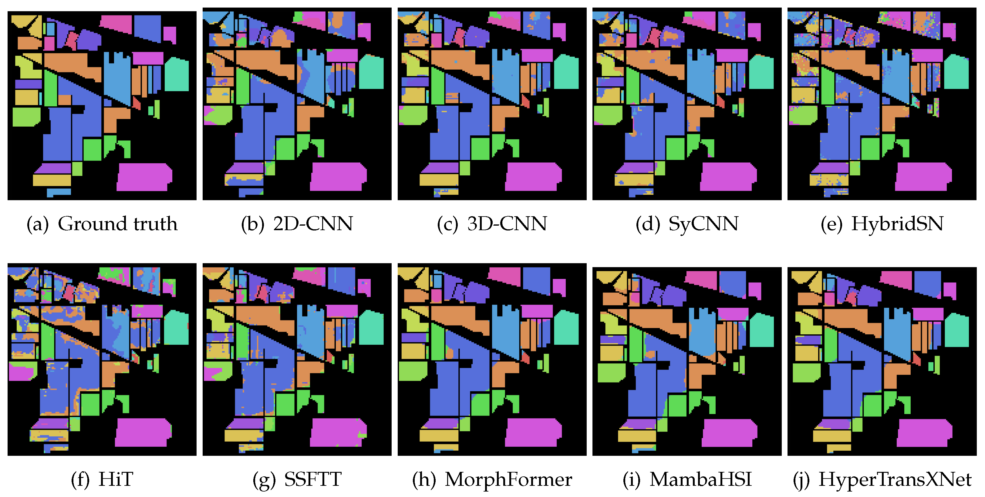
• The Indian Pines Scene dataset was collected by the AVIRIS sensor in 1992 in the northwestern part of Indiana, USA. It contains hyperspectral image data with a spatial resolution of $145\times 145$ and 220 spectral bands. During preprocessing, 20 noisy bands were removed, leaving 200 valid bands for analysis. The dataset includes 16 land-cover classes, such as Alfalfa, Corn, and Woods, and is widely used in hyperspectral image classification tasks. In the experiment, 10% of the samples were randomly selected for training, and the remaining 90% were used for testing to evaluate the model’s performance.
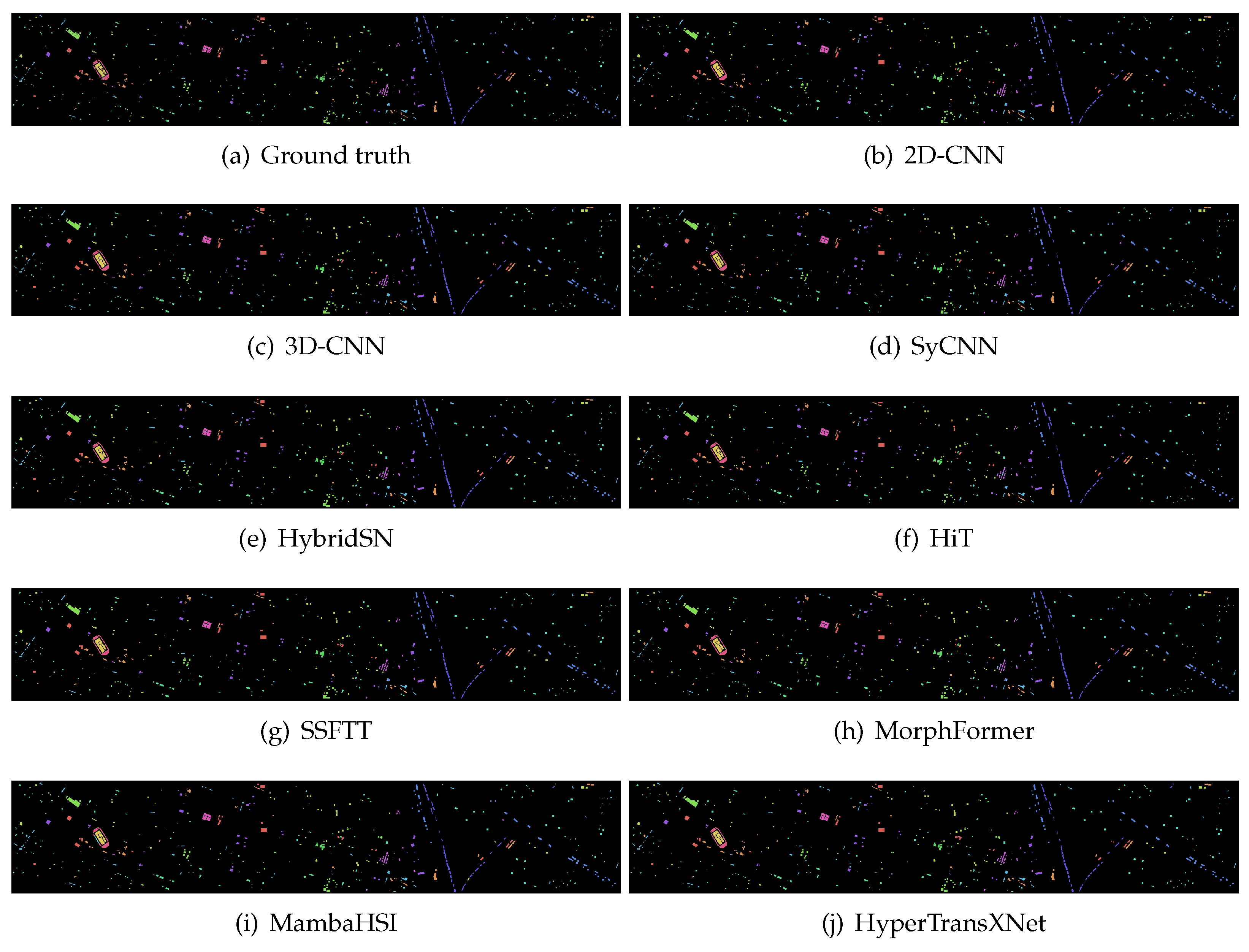
• Houston 2013 dataset: This dataset encompasses the geographical information of Houston, Texas, USA, and its surrounding areas, acquired using the ITRES CASI-1500 imaging spectrometer. It features a spatial resolution of $349\times 1905$ pixels and covers 144 spectral bands. The dataset is based on a high-quality, cloud-free image provided by the Geo-Science and Remote Sensing Society (GRRSS). It contains 15 distinct land-use categories, such as highways, roads, and vegetation. In our experimental setup, we randomly selected 10% of the dataset for model training, with the remaining 90% reserved for validation and testing.
• The WHU-HI-Longkou (WHL) dataset was collected on 17 July 2018, in Longkou Town, Hubei Province, China, using a DJI M600 Pro drone equipped with a Headwall Nano Hyperspectral Imaging Sensor. The sensor has an 8 mm focal length, and the drone flew at an altitude of 500 m, capturing images with a resolution of $550\times 400$ pixels and covering 270 spectral bands, with wavelengths ranging from 400 to 1000 nm. The dataset includes nine land cover types with a total of 204,542 labeled samples, providing rich hyperspectral information for classification method evaluation. In this study, 1% of the labeled samples were used for training, and the remaining 99% for testing, simulating classification tasks with limited labeled data to assess the model’s generalization ability in small sample learning.

5.1.2. Evaluation Metrics

The classification performance was evaluated using three commonly employed metrics: overall accuracy (OA), average accuracy (AA), and the Kappa coefficient ($\kappa$).

5.1.3. Comparison Methods

Comparison methods: We choose seven state-of-the-art methods to compare with HyperTransXNet, including CNNs (e.g., 2D-CNN [43], 3D-CNN [3], and Hybridsn [6]), Transformers (such as HiT [32], MorphFormer [31], and SSFTT [7]), and Mamba (Mambahsi [44]).

5.1.4. Setting

During training, we randomly extracted 100 patches of size $15\times 15$ as input data. We set the total number of iterations to 100 and employed all comparison methods alongside HyperTransXNet using the PyTorch (version 2.6.0) framework. HyperTransXNet was optimized using the Adam optimizer with a learning rate of $1\times {10}^{-3}$ and a batch size of 100.

5.2. Results and Analysis

We conducted experiments on three widely used HSI datasets and evaluated their performance using two metrics. The results, presented in

Table 1. Comparison with the state-of-the-art CNNs and Transformers on the Indian Pines Scene dataset (10% training samples).

Class	2D-CNN	3D-CNN	Hybridsn	HiT	SSFTT	Morphformer	MambaHSI	HyperTransXNet
Alfalfa	92.82 ± 4.80	69.95 ± 17.92	18.85 ± 29.79	16.34 ± 15.70	89.65 ± 6.91	82.13 ± 22.40	76.83 ± 22.15	89.51 ± 14.39
Corn-notill	93.81 ± 1.97	88.61 ± 1.17	84.84 ± 11.22	90.48 ± 1.22	94.11 ± 1.08	93.38 ± 2.14	90.97 ± 3.50	94.23 ± 1.72
Corn-mintill	92.19 ± 1.77	86.74 ± 1.90	75.93 ± 18.40	93.13 ± 3.63	90.13 ± 2.66	91.28 ± 3.66	90.46 ± 5.05	96.22 ± 2.30
Corn	97.94 ± 1.50	93.92 ± 2.44	80.93 ± 17.01	91.17 ± 5.12	94.90 ± 3.46	95.26 ± 4.04	90.38 ± 6.24	93.90 ± 5.63
Grass-pasture	93.09 ± 3.32	93.44 ± 0.70	73.56 ± 16.43	81.89 ± 10.59	93.08 ± 2.52	94.72 ± 1.55	95.26 ± 2.14	95.61 ± 2.37
Grass-trees	95.65 ± 2.97	94.82 ± 0.67	75.90 ± 15.75	95.11 ± 0.98	95.98 ± 1.29	95.47 ± 1.38	94.70 ± 2.37	97.26 ± 1.22
Grass-pasture-mowed	7.94 ± 18.29	0.00 ± 0.00	0.00 ± 0.00	0.00 ± 0.00	54.69 ± 35.84	71.56 ± 18.01	44.40 ± 32.52	28.40 ± 30.54
Hay-windrowed	99.69 ± 0.55	98.87 ± 1.10	87.72 ± 13.09	99.86 ± 0.21	98.77 ± 1.35	99.81 ± 0.39	99.72 ± 0.46	100.00 ± 0.00
Oats	73.30 ± 29.09	0.00 ± 0.00	2.45 ± 5.09	0.00 ± 0.00	54.34 ± 32.04	21.28 ± 30.14	57.22 ± 25.95	50.56 ± 36.47
Soybean-notill	87.78 ± 1.60	83.25 ± 1.22	78.05 ± 9.87	77.61 ± 2.07	87.11 ± 1.77	88.80 ± 3.58	84.25 ± 5.74	83.09 ± 2.03
Soybean-mintill	96.26 ± 1.24	94.38 ± 0.51	91.41 ± 4.16	96.09 ± 1.74	96.78 ± 0.82	96.27 ± 0.59	96.12 ± 3.54	98.40 ± 0.54
Soybean-clean	91.80 ± 2.21	89.11 ± 1.71	78.53 ± 12.76	91.18 ± 3.46	89.52 ± 3.35	87.66 ± 5.08	92.96 ± 5.99	93.16 ± 4.09
Wheat	98.12 ± 1.32	86.71 ± 7.81	54.68 ± 33.43	91.89 ± 2.96	95.00 ± 3.62	94.35 ± 4.88	95.14 ± 2.90	90.76 ± 5.41
Woods	98.28 ± 2.42	97.81 ± 0.58	94.10 ± 5.22	99.45 ± 0.38	98.67 ± 0.66	98.87 ± 0.31	99.16 ± 0.43	99.49 ± 0.39
Buildings-Grass-Trees-Drives	97.82 ± 1.46	93.48 ± 2.25	73.19 ± 17.09	87.90 ± 11.83	96.08 ± 2.76	96.06 ± 1.48	90.86 ± 4.12	96.31 ± 3.60
Stone-Steel-Towers	52.74 ± 21.39	46.87 ± 17.62	41.04 ± 32.91	16.79 ± 20.55	39.20 ± 32.30	25.11 ± 33.4	22.98 ± 18.69	45.36 ± 17.65
OA (%)	94.48 ± 1.41	91.48 ± 0.52	83.10 ± 10.19	90.85 ± 1.13	94.09 ± 0.97	94.03 ± 0.90	92.72 ± 1.15	94.74 ± 0.39
AA (%)	83.81 ± 3.38	73.92 ± 2.12	62.87 ± 12.02	70.56 ± 2.84	84.54 ± 3.91	82.75 ± 2.85	82.59 ± 3.35	84.52 ± 2.76
$\kappa$ (%)	93.69 ± 1.61	90.25 ± 0.59	80.70 ± 11.52	89.53 ± 1.31	93.25 ± 1.10	93.18 ± 1.03	91.69 ± 1.30	93.99 ± 0.44

,

Table 2. Comparison with the state-of-the-art CNNs and Transformers on the Houston 2013 dataset (10% training samples).

Class	2D-CNN	3D-CNN	HybridSN	HiT	SSFTT	Morphformer	MambaHSI	HyperTransXNet
Healthy Grass	95.21 ± 1.66	91.06 ± 3.44	90.76 ± 1.88	90.02 ± 3.40	96.42 ± 1.16	85.97 ± 8.75	96.94 ± 1.80	98.41 ± 1.19
Stressed grass	95.51 ± 1.72	88.85 ± 6.46	86.26 ± 8.27	95.63 ± 0.83	97.16 ± 1.42	88.97 ± 5.58	94.21 ± 2.69	97.25 ± 2.50
Synthetic GrassTrees	99.24 ± 0.45	97.36 ± 3.06	95.85 ± 3.67	97.48 ± 0.66	99.30 ± 0.58	91.37 ± 13.84	97.26 ± 1.06	97.62 ± 0.73
Trees	94.72 ± 2.18	88.28 ± 4.52	79.71 ± 7.46	87.64 ± 4.96	97.68 ± 0.90	90.96 ± 4.95	94.49 ± 2.31	96.98 ± 1.97
Soil	99.81 ± 0.17	95.72 ± 3.71	96.41 ± 3.83	99.90 ± 0.14	99.43 ± 0.63	97.96 ± 2.17	99.63 ± 0.38	99.97 ± 0.04
Water	94.05 ± 0.97	86.16 ± 1.92	91.69 ± 3.12	74.69 ± 3.14	93.61 ± 3.07	90.85 ± 4.25	90.86 ± 6.69	92.57 ± 3.57
Residential	96.82 ± 1.02	83.00 ± 6.98	78.74 ± 17.12	73.54 ± 8.98	97.52 ± 0.80	85.78 ± 24.73	95.88 ± 1.52	98.89 ± 0.68
Commercial	97.62 ± 1.51	89.55 ± 1.61	93.01 ± 2.65	87.67 ± 4.75	97.88 ± 1.24	90.76 ± 9.56	96.46 ± 1.38	96.06 ± 1.43
Road	95.42 ± 1.51	85.03 ± 3.38	73.95 ± 14.36	81.45 ± 3.15	96.70 ± 1.56	87.54 ± 7.99	96.16 ± 1.59	99.00 ± 0.90
Highway	99.09 ± 1.57	91.67 ± 6.54	91.92 ± 7.92	96.51 ± 2.25	99.78 ± 0.38	93.89 ± 9.76	99.94 ± 0.19	100.00 ± 0.00
Railway	99.58 ± 0.46	81.57 ± 5.87	85.29 ± 7.92	93.82 ± 3.78	99.76 ± 0.44	91.69 ± 16.26	97.00 ± 1.92	99.62 ± 0.80
Parking Lot 1	97.88 ± 1.83	94.30 ± 1.81	95.79 ± 2.71	93.77 ± 3.09	98.70 ± 1.24	88.63 ± 13.89	97.32 ± 1.71	99.22 ± 0.84
Parking Lot 2	97.55 ± 2.44	81.89 ± 6.24	86.51 ± 8.08	90.28 ± 3.60	98.54 ± 1.23	92.25 ± 6.66	97.27 ± 1.79	98.13 ± 2.36
Tennise Court	99.98 ± 0.07	98.60 ± 0.97	92.98 ± 6.16	99.82 ± 0.55	99.67 ± 0.47	99.04 ± 1.46	99.77 ± 0.50	100.00 ± 0.00
Running Track	97.87 ± 1.71	94.77 ± 5.41	91.48 ± 5.60	99.21 ± 1.37	98.95 ± 0.71	93.32 ± 7.49	97.17 ± 4.63	100.00 ± 0.00
OA (%)	97.32 ± 0.48	89.54 ± 3.21	88.19 ± 4.75	90.67 ± 1.01	98.15 ± 0.53	90.98 ± 7.71	96.80 ± 0.55	98.46 ± 0.29
AA (%)	97.03 ± 0.37	89.74 ± 2.87	88.97 ± 4.09	90.76 ± 0.92	97.81 ± 0.59	90.99 ± 7.46	96.69 ± 0.69	98.25 ± 0.22
$\kappa (\%)$	97.10 ± 0.51	88.70 ± 3.47	87.24 ± 5.13	89.91 ± 1.09	98.00 ± 0.58	90.24 ± 8.36	96.54 ± 0.59	98.33 ± 0.31

and

Table 3. Comparison with the state-of-the-art CNNs and Transformers on the WHL dataset (1% training samples).

Class	2D-CNN	3D-CNN	HybridSN	HiT	SSFTT	Morphformer	MambaHSI	HyperTransXNet
Corn	99.87 ± 0.03	99.34 ± 0.40	99.34 ± 0.58	99.79 ± 0.08	99.88 ± 0.04	99.89 ± 0.06	99.73 ± 0.24	99.84 ± 0.11
Cotton	99.72 ± 0.09	96.30 ± 1.24	97.55 ± 3.18	97.26 ± 2.05	99.69 ± 0.11	99.78 ± 0.13	99.78 ± 0.25	99.19 ± 0.75
Sesame	94.97 ± 1.27	55.88 ± 29.79	81.52 ± 14.54	94.55 ± 3.24	98.93 ± 0.54	99.44 ± 0.42	95.44 ± 1.70	98.82 ± 0.77
Broad-leaf soybean	99.12 ± 0.08	96.24 ± 0.89	98.22 ± 0.64	99.77 ± 0.10	99.63 ± 0.05	99.65 ± 0.16	99.61 ± 0.22	99.83 ± 0.13
Narrow-leaf soybean	95.42 ± 0.71	87.80 ± 2.44	81.06 ± 10.19	88.16 ± 3.47	98.30 ± 0.48	97.60 ± 1.50	95.25 ± 3.24	96.38 ± 1.97
Rice	98.57 ± 0.19	98.11 ± 0.66	97.28 ± 0.91	99.36 ± 0.19	98.96 ± 0.44	99.05 ± 0.23	98.33 ± 0.72	98.54 ± 0.49
Water	99.74 ± 0.04	99.51 ± 0.22	97.11 ± 0.53	99.99 ± 0.01	99.56 ± 0.12	99.49 ± 0.15	99.86 ± 0.11	99.85 ± 0.10
Roads and houses	85.56 ± 0.78	82.84 ± 2.22	78.60 ± 7.09	84.38 ± 3.87	89.32 ± 2.82	91.03 ± 1.82	87.57 ± 3.60	87.32 ± 2.85
Mixed weed	78.58 ± 2.04	79.05 ± 2.99	37.10 ± 12.86	70.44 ± 3.65	84.48 ± 3.09	83.76 ± 1.79	86.64 ± 5.89	88.04 ± 4.99
OA(%)	98.35 ± 0.09	96.60 ± 0.63	95.77 ± 0.80	98.12 ± 0.14	98.86 ± 0.20	98.74 ± 0.16	98.74 ± 0.22	98.91 ± 0.16
AA (%)	93.24 ± 0.46	84.58 ± 3.95	82.29 ± 3.59	92.63 ± 0.80	95.72 ± 0.72	95.03 ± 0.67	95.80 ± 0.94	96.42 ± 0.69
$\kappa (\%)$	97.82 ± 0.13	95.49 ± 0.85	94.38 ± 1.07	97.52 ± 0.19	98.50 ± 0.26	98.34 ± 0.21	98.35 ± 0.29	98.57 ± 0.21

(with the best values highlighted in bold), reveal that the proposed HyperTransXNet achieves superior classification accuracy across all datasets. This performance is primarily attributed to two key innovations. First, HyperTransXNet incorporates a Hybrid Spatial-Spectral Module (HSSM) that employs parallel local dynamic convolutions alongside global frequency-domain attention mechanisms, thereby capturing both fine-grained spatial details and broader spectral correlations. Second, the architecture integrates a Mixture-of-Experts Routing mechanism (MoE-R) that adaptively fuses multi-scale features through a learnable routing process. Notably, HyperTransXNet delivers satisfactory classification outcomes on the unbalanced WHU-HI-Longkou dataset and demonstrates enhanced performance across nearly all categories.

An additional observation is that Transformer architectures augmented with local feature extraction components (e.g., SSFTT, HiT, and MorphFormer) demonstrably outperform conventional Transformer models (e.g., ViT and DeepViT). This advantage arises because, although traditional Transformers effectively capture global representations from patch embeddings, they often fall short in emphasizing localized features. In contrast, while straightforward feature fusion strategies may introduce noise and redundancy, the integration of local features with global representations occurs in HyperTransXNet. For example, on the Indian Pines dataset, HyperTransXNet achieved a classification accuracy of 94.74%, surpassing the 94.03% of MorphFormer by 0.71%, thereby underscoring the efficacy of combining local and global feature representations.

Furthermore, convolutional neural networks (CNNs), as classical deep learning models, excel in image processing tasks due to their proficiency in extracting local features. However, their focus on local connectivity limits their ability to capture long-range dependencies and global contextual relationships, as evidenced by our experimental comparisons. Specifically, on the Houston 2013 dataset, HyperTransXNet achieved an accuracy of 98.46%, outperforming traditional 2D-CNN and 3D-CNN models. This notable improvement emphasizes the critical importance of integrating both local and global features and highlights the potential for further architectural enhancements in CNN frameworks.

In addition, the recently introduced Mamba series models have emerged as promising deep learning architectures with significant advantages in hyperspectral image (HSI) classification. These models have achieved breakthroughs in multi-scale feature extraction by innovatively integrating the Selective State Space Model (SSM) with a dynamic scanning mechanism. Their architectural design combines the strengths of convolutional neural networks (CNNs) in local feature extraction with the robust global context modeling capabilities of Transformer architectures. However, a fundamental limitation of these models is the absence of an explicit feature fusion module, necessitating external components for effective feature integration in tasks that demand complex feature collaboration. Analysis of experimental results reveals that the proposed HyperTransXNet, an advanced architecture that effectively fuses both local and global features, outperforms the Mamba series models. For example, on the Houston 2013 dataset, HyperTransXNet achieves a 1.66% higher overall accuracy compared to Mambahsi. This outcome underscores the importance of incorporating a fusion module and further demonstrates the potential of the Mamba series models in the realm of HSI classification.

Figure 5, Figure 6 and Figure 7 present a comparative performance analysis of the proposed HyperTransXNet method across three widely adopted benchmark datasets in remote sensing image analysis: the Indian Pines scene, Houston 2013, and WHU-HI-Longkou datasets. The visual outcomes clearly demonstrate that HyperTransXNet achieves exceptionally high classification accuracy across all categories. Moreover, the classification maps produced by the model exhibit strong concordance with the ground truth, indicating that HyperTransXNet effectively integrates both local features and global representations. This superior performance can be primarily attributed to the design of HyperTransXNet, which is specifically optimized for the fusion of heterogeneous features, thereby significantly enhancing classification performance. A detailed examination of the comparative charts reveals that most alternative methods yield classification maps with substantial noise levels, a finding that corresponds with the quantitative results summarized in previous tables. This observation suggests that conventional convolutional neural networks (CNNs), frequently employed in computer vision tasks, often encounter difficulties in capturing global representations. Similarly, recent transformer-based models, despite their rising prominence, also face challenges in effectively merging local and global features.

These results underscore the necessity of developing methodologies that can adeptly balance the integration of local and global features in remote sensing image classification tasks, thereby enhancing overall performance. In summary, through its innovative architectural design, HyperTransXNet not only overcomes the limitations of traditional feature fusion methods but also offers a more efficient and accurate solution for remote sensing image classification.

To comprehensively evaluate the feature representation capabilities of the proposed HyperTransXNet method, we conducted a t-SNE visualization comparative analysis against six benchmark methods: CNN-based approaches (2D-CNN and HybridSN), visual Transformer series models (SSFTT and MorphFormer), and Mamba series models (Mambahsi). Figure 8 displays the t-SNE visualization results of each method on the Indian Pines dataset, a widely used resource in remote sensing image analysis due to its rich hyperspectral information and diverse land cover types. The visualization clearly indicates that HyperTransXNet outperforms the other methods in terms of clustering performance within the feature space, with its t-SNE map exhibiting more compact intra-class clusters and more distinct inter-class boundaries. This superior performance primarily arises from the model’s unique architectural design, where the integration of a global frequency domain attention mechanism with local dynamic convolution effectively captures both global dependencies and local contextual information in hyperspectral images. Such capabilities are essential for accurately identifying land cover categories characterized by complex spectral features. In contrast, traditional convolutional neural networks, constrained by limited long-range dependency modeling, demonstrate more dispersed cluster distributions and substantial inter-class interference. Transformer-based models, despite improvements in processing global information, still reveal limitations in capturing fine-grained local details, as evidenced by less cohesive intra-class aggregation and noticeable misclassification. Mamba series models, which typically employ unidirectional or bidirectional global scanning without targeted modeling of local spatial-spectral cubes, struggle to capture subtle local features, resulting in inadequate intra-class cohesion and pronounced misclassification. This visualization analysis not only corroborates the outstanding performance of HyperTransXNet in hyperspectral classification tasks but also provides intuitive evidence of its advantages, thereby reinforcing its effectiveness in feature representation and establishing a robust theoretical foundation for its broad application in remote sensing image analysis.

5.3. Comparison of Computational Complexity

This study presents a computational complexity analysis of various comparison methods alongside the HyperTransXNet network, all assessed using the Houston 2013 dataset. As detailed in

Table 4. Comparison of computational complexity.

Methods	FLOPs (G)	Param (MB)	Inference Speed (sample/s)	Peak Memory (MB)	Training Time (s)	Testing Time (s)	OA (%)	AA (%)	$\mathit{\kappa }$ (%)
ViT	2.71	52.22	565.30	715.06	727.89	3.43	90.27 ± 1.69	90.45 ± 1.42	89.48 ± 1.83
DeepViT	2.71	52.22	352.53	881.06	1497.97	6.82	91.58 ± 1.50	91.38 ± 1.43	90.89 ± 1.62
CvT	9.04	17.77	149.52	8494.94	2758.06	11.65	93.52 ± 1.88	93.75 ± 1.95	92.99 ± 2.04
HiT	1.81	16.94	103.91	8314.00	112.04	6.7	95.20 ± 0.33	94.80 ± 0.32	94.81 ± 0.35
SSFTT	0.97	87.04	148.29	8198.00	389.62	1.59	98.15 ± 0.53	97.82 ± 0.59	98.00 ± 0.58
MorphFormer	0.74	87.04	11.44	8200.00	874.99	4.16	90.98 ± 7.71	90.99 ± 7.46	90.24 ± 8.36
MambaHSI	0.006	0.10	440.88	8202.00	170.71	0.10	96.80 ± 0.55	96.69 ± 0.69	96.54 ± 0.59
HyperTransXNet	0.24	1.08	278.63	707.06	201.39	0.13	98.46 ± 0.29	98.25 ± 0.22	98.33 ± 0.31

, HyperTransXNet exhibits considerable advantages while maintaining high classification accuracy. We can observe that its overall accuracy (OA) reaches 98.46% and its Kappa coefficient is 98.33%, outperforming current mainstream Transformer architectures. Notably, HyperTransXNet achieves the highest OA performance with only 1.08 MB of parameters.

The computational complexity analysis further indicates that the CvT network requires $9.04$ G floating-point operations (FLOPs) and a training time of 2758.06 s (approximately 46 min), with its high computational density and parameter count (17.77 MB) potentially leading to training efficiency bottlenecks. In contrast, HyperTransXNet completes training in just $201.39$ s, utilizing only $0.24$ FLOPs and $1.08$ of parameters, while its testing time is limited to $0.13$ s. At the same time, its memory consumption is only 707.06 MB, which is the lowest among all comparison models. This optimized balance between accuracy and efficiency renders the approach highly applicable to hyperspectral classification scenarios that demand real-time processing.

5.4. Ablation Studies

Ablation study of the input size: 

Table 5. Study of the input size.

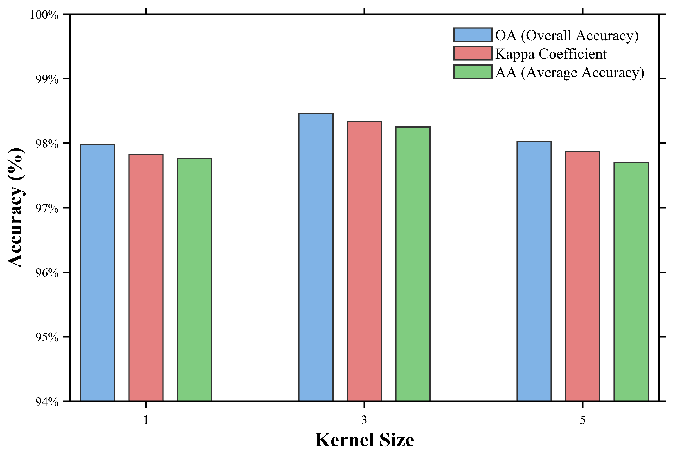
Sizes	IndianPines		WHU-HI-Longkou		Houston2013
	OA	Kapp	OA	Kapp	OA	Kapp
$11\times 11$	97.43 ± 0.34	97.07 ± 0.39	99.25 ± 0.08	99.01 ± 0.11	98.78 ± 0.27	98.69 ± 0.29
$13\times 13$	95.82 ± 0.51	95.23 ± 0.58	99.14 ± 0.18	98.87 ± 0.23	98.50 ± 0.30	98.38 ± 0.33
$15\times 15$	94.74 ± 0.39	93.99 ± 0.44	98.91 ± 0.16	98.57 ± 0.21	98.46 ± 0.29	98.33 ± 0.31
$17\times 17$	92.88 ± 0.63	91.86 ± 0.71	98.49 ± 0.29	98.01 ± 0.38	98.14 ± 0.35	97.99 ± 0.38
$19\times 19$	91.12 ± 1.53	89.85 ± 1.74	98.27 ± 0.13	97.72 ± 0.17	97.58 ± 0.23	97.38 ± 0.25

presents an investigation into the impact of input size on the classification performance across three datasets. By varying the input size from $11\times 11$ to $19\times 19$, the resulting classification accuracies, as detailed in Table 5, demonstrate that performance varies significantly with different input dimensions. Notably, smaller input sizes yield higher overall accuracy (OA) and Kappa coefficients, likely because they facilitate the extraction of more precise features, thereby enhancing the identification of land cover types. Conversely, larger input sizes may introduce extraneous noise. These findings further substantiate the robustness of the proposed HyperTransXNet method. Consequently, to comprehensively evaluate HyperTransXNet, the input size was optimally set to $15\times 15$.

Ablation study of different modules: 

Table 6. Study of different modules.

Methods	SSLB	SSGB	OA (%)	$\mathit{\kappa }$ (%)
2D-CNN	×	×	97.32 ± 0.48	97.10 ± 0.51
HyperTransXNet	√	×	98.05 ± 0.43 (↑0.73%)	97.89 ± 0.46 (↑0.79%)
HyperTransXNet	×	√	98.18 ± 0.25 (↑0.86%)	98.04 ± 0.27 (↑0.94%)

presents an ablation study assessing the impacts of the SSLB and SSGB configurations on the Houston 2013 dataset, with the 2D-CNN serving as the baseline method. As shown in Table 6, the proposed models (HyperTransXNet_SSLB and HyperTransXNet_SSGB) outperform the conventional 2D-CNN in terms of overall accuracy (OA) and the Kappa coefficient. Specifically, HyperTransXNet_SSLB improves OA by 0.73% and the Kappa coefficient by 0.79%, while HyperTransXNet_SSGB achieves improvements of 0.86% in OA and 0.94% in the Kappa coefficient relative to the 2D-CNN. This enhancement is attributed to the SSLB module’s ability to effectively capture local contextual features and the SSGB module’s strength in modeling global dependency relationships. These findings underscore that integrating optimal local contextual features with global dependencies significantly enhances classification performance.

Ablation study of SSTE: In order to verify the superiority of the proposed SSTE module for feature fusion,

Table 7. Study of SSTE.

Methods	SSTE	OA (%)	$\mathit{\kappa }$ (%)
HyperTransXNet_SSLB_SSGB	×	98.16 ± 0.32	98.01 ± 0.34
HyperTransXNet_SSLB_SSGB	√	98.46 ± 0.29 (↑0.30%)	98.33 ± 0.31 (↑0.32%)

presents the ablation study results on the Houston 2013 dataset. The experimental results indicate that the model enhanced with SSTE: achieves superior performance in both overall accuracy (OA) and the Kappa coefficient. Notably, the HyperTransXNet_SSLB_SSGB_SSTE model shows improvements of 0.30% in OA and 0.32% in $\kappa$ compared to the HyperTransXNet_SSLB_SSGB. These findings not only validate the effectiveness of SSTE in integrating corresponding local features with the global representation but also underscore the merits of incorporating this module.

Ablation study of SSTE and MoE-R: In

Table 8. Study of SSTE and MoE-R.

Methods	SSTE	MoE-R	OA (%)	$\mathit{\kappa }$ (%)
HyperTransXNet_SSLB_SSGB	×	√	93.73 ± 1.53	93.22 ± 1.65
HyperTransXNet_SSLB_SSGB	√	×	98.46 ± 0.29 (↑4.73%)	98.33 ± 0.31 (↑5.11%)

, we conducted an ablation study on the SSTE and MoE-R modules using the Houston 2013 dataset. The results indicate that HyperTransXNet_SSLB_SSGB_SSTE significantly outperforms HyperTransXNet_SSLB_SSGB_MoE-R in terms of OA (4.73%) and $\kappa$ (5.11%). This superior performance can be attributed to the ability of SSTE to achieve channel alignment through $1\times 1$ convolution, which ensures consistent dimensions during feature fusion by MoE-R. Additionally, SSTE effectively preserves the original distribution of features through residual connections. The experimental results confirm that SSTE and MoE-R exhibit a complementary relationship rather than redundancy.

Ablation study of the dynamic kernel size in the HSSM: By default, we set the dynamic kernel size (K) in HSSM to 3. Since variations in kernel size can significantly impact the performance of the module, we conducted experiments to assess the effects of different kernel sizes on overall accuracy (OA), specifically using sizes of 1, 3, and 5. As shown in Figure 9, $K=3$ achieved the highest classification accuracy (OA = 98.46%) on the Houston 2013 dataset. In contrast, $K=1$ and $K=5$ resulted in performance declines of 0.48% (vs. 97.98%) and 0.43% (vs. 98.03%), respectively, with the model’s OA fluctuation remaining below 0.5%. According to the experimental results, the robustness of the model under varying kernel sizes is fully demonstrated.

Ablation study of the expert count in the MoE-R: We set the expert count (E) in the Mixture-of-Experts Routing mechanism (MoE-R) to 4 by default. To validate this choice, we evaluated the impact of different expert counts; specifically, $E\in \{2,4,8\}$ on parameter efficiency and overall accuracy (OA) using the Houston 2013 dataset. As shown in

Table 9. Impact of different expert counts for the OA and parameter efficiency.

Number of Experts (E)	FLOPs (G)	Param (MB)	Parameter Efficiency (Acc/Param)	Marginal Parameter Efficiency ($\mathsf{\Delta }$ Acc/$\mathsf{\Delta }$ Param)	OA (%)	AA (%)	$\mathit{\kappa }$ (%)
2	0.21	0.99	99.05	-	98.06 ± 0.44	97.63 ± 0.39	97.90 ± 0.48
4	0.24	1.08	91.17	4.44	98.46 ± 0.29	98.25 ± 0.22	98.33 ± 0.31
8	0.30	1.26	77.75	−2.78	97.96 ± 0.49	97.51 ± 0.54	97.80 ± 0.53

, increasing E from 2 to 4 resulted in an improvement in OA by 0.40% with a Marginal Parameter Efficiency (MPE) of 4.44. Conversely, increasing E from 4 to 8 led to a decrease in OA by 0.50%, accompanied by a negative MPE of −2.78. These results demonstrate that $E=4$ optimally balances MPE (4.44) and OA (98.46%), confirming the scientific rationale behind our default selection and indicating model robustness, as evidenced by an OA fluctuation of ≤0.50%, even with suboptimal E values.

Ablation study of training sample ratio: This study investigates the impact of training sample ratio on the classification performance of three hyperspectral benchmark datasets. To evaluate the model’s performance across varying levels of data availability, we selected a small sample size of 5%, representing an extreme scenario in which resources are severely limited in real-world applications. Additionally, we included sample sizes ranging from 20% to 50% to identify the saturation point of model performance. According to Figure 10, there is a significant positive correlation between overall classification accuracy (OA) and the number of training samples. For instance, in the Indian Pines dataset, the OA increased from 94.74% to 95.84% as the number of training samples gradually increased. This trend indicates that the model’s ability to capture a consistent data distribution improves with the expansion of the training scale. Similarly, in the Houston 2013 dataset, the OA rose from 98.46% to 99.41%, further confirming that sufficient training data enhances the model’s cross-class generalization ability. These findings suggest that increasing the number of training samples not only mitigates the impact of intra-class feature heterogeneity but also improves the model’s capacity to delineate inter-class decision boundaries. Overall, this study provides valuable insights for hyperspectral classification tasks, indicating that expanding the training dataset significantly enhances the robustness and reliability of the classification system by strengthening the model’s structured representation of the feature space.

6. Conclusions

In this study, we leverage the advantages of CNNs and vision Transformers to propose a novel hybrid network, HyperTransXNet, for hyperspectral image (HSI) classification. Unlike previous approaches, we introduce a HSSM that synergistically combines global frequency-domain attention mechanisms with local dynamic convolutions, enabling the effective capture of both global dependencies and local contextual information in hyperspectral imagery. To adaptively fuse the corresponding local features and global representations, we further propose an SSTE mechanism for robust information integration. Extensive experiments demonstrate that our proposed HyperTransXNet outperforms state-of-the-art CNNs and vision Transformers. In future work, we aim to explore additional fusion modules to further enhance the learning capabilities of Transformers.

References

- Kang, X.; Wang, Z.; Duan, P.; Wei, X. The potential of hyperspectral image classification for oil spill mapping. IEEE Trans. Geosci. Remote Sens. 2022, 60, 1–15. [Google Scholar]
- Chen, F.; Wang, K.; Van de Voorde, T.; Tang, T.F. Mapping urban land cover from high spatial resolution hyperspectral data: An approach based on simultaneously unmixing similar pixels with jointly sparse spectral mixture analysis. Remote Sens. Environ. 2017, 196, 324–342. [Google Scholar]
- Yang, X.; Zhang, X.; Ye, Y.; Lau, R.Y.; Lu, S.; Li, X.; Huang, X. Synergistic 2D/3D convolutional neural network for hyperspectral image classification. Remote Sens. 2020, 12, 2033. [Google Scholar]
- Shen, J.; Zhang, D.; Dong, G.; Sun, D.; Liang, X.; Su, M. Classification of hyperspectral images based on fused 3D inception and 3D-2D hybrid convolution. Signal Image Video Process. 2024, 18, 3031–3041. [Google Scholar]
- Paoletti, M.E.; Haut, J.M.; Plaza, J.; Plaza, A. Deep dense convolutional neural network for hyperspectral image classification. Remote Sens. 2018, 10, 1454. [Google Scholar]
- Roy, S.K.; Krishna, G.; Dubey, S.R.; Chaudhuri, B.B. HybridSN: Exploring 3-D–2-D CNN feature hierarchy for hyperspectral image classification. IEEE Geosci. Remote Sens. Lett. 2019, 17, 277–281. [Google Scholar]
- Sun, L.; Zhao, G.; Zheng, Y.; Wu, Z. Spectral–spatial feature tokenization transformer for hyperspectral image classification. IEEE Trans. Geosci. Remote Sens. 2022, 60, 5522214. [Google Scholar]
- Yao, J.; Hong, D.; Li, C.; Chanussot, J. Spectralmamba: Efficient mamba for hyperspectral image classification. arXiv 2024, arXiv:2404.08489. [Google Scholar]
- Sheng, J.; Zhou, J.; Wang, J.; Ye, P.; Fan, J. Dualmamba: A lightweight spectral-spatial mamba-convolution network for hyperspectral image classification. IEEE Trans. Geosci. Remote Sens. 2024, 63, 5501415. [Google Scholar]
- Li, Y.; Zhang, H.; Shen, Q. Spectral-spatial classification of hyperspectral imagery with 3D convolutional neural network. Remote Sens. 2017, 9, 67. [Google Scholar]
- Xu, H.; Yao, W.; Cheng, L.; Li, B. Multiple spectral resolution 3D convolutional neural network for hyperspectral image classification. Remote Sens. 2021, 13, 1248. [Google Scholar]
- Ghaderizadeh, S.; Abbasi-Moghadam, D.; Sharifi, A.; Zhao, N.; Tariq, A. Hyperspectral image classification using a hybrid 3D-2D convolutional neural networks. IEEE J. Sel. Top. Appl. Earth Obs. Remote Sens. 2021, 14, 7570–7588. [Google Scholar]
- Zhang, H.; Li, Y.; Zhang, Y.; Shen, Q. Spectral-spatial classification of hyperspectral imagery using a dual-channel convolutional neural network. Remote Sens. Lett. 2017, 8, 438–447. [Google Scholar]
- Haque, M.R.; Mishu, S.Z.; Palash Uddin, M.; Al Mamun, M. A lightweight 3D-2D convolutional neural network for spectral-spatial classification of hyperspectral images. J. Intell. Fuzzy Syst. 2022, 43, 1241–1258. [Google Scholar]
- Luo, Y.; Zou, J.; Yao, C.; Zhao, X.; Li, T.; Bai, G. HSI-CNN: A novel convolution neural network for hyperspectral image. In Proceedings of the 2018 International Conference on Audio, Language and Image Processing (ICALIP), Shanghai, China, 16–17 July 2018; pp. 464–469. [Google Scholar]
- Liang, L.; Zhang, S.; Li, J.; Plaza, A.; Cui, Z. Multi-scale spectral-spatial attention network for hyperspectral image classification combining 2D octave and 3D convolutional neural networks. Remote Sens. 2023, 15, 1758. [Google Scholar]
- Diakite, A.; Jiangsheng, G.; Xiaping, F. Hyperspectral image classification using 3D 2D CNN. IET Image Process. 2021, 15, 1083–1092. [Google Scholar]
- Cao, J.; Li, X. A 3D 2D convolutional neural network model for hyperspectral image classification. arXiv 2021, arXiv:2111.10293. [Google Scholar]
- Liu, H.; Li, W.; Xia, X.G.; Zhang, M.; Gao, C.Z.; Tao, R. Central Attention Network for Hyperspectral Imagery Classification. IEEE Trans. Neural Netw. Learn. Syst. 2023, 34, 8989–9003. [Google Scholar] [CrossRef]
- Liu, H.; Li, W.; Xia, X.G.; Zhang, M.; Tao, R. Multiarea Target Attention for Hyperspectral Image Classification. IEEE Trans. Geosci. Remote Sens. 2023, 61, 5524916. [Google Scholar] [CrossRef]
- Mei, S.; Li, X.; Liu, X.; Cai, H.; Du, Q. Hyperspectral image classification using attention-based bidirectional long short-term memory network. IEEE Trans. Geosci. Remote Sens. 2021, 60, 5509612. [Google Scholar]
- Ayas, S.; Tunc-Gormus, E. SpectralSWIN: A spectral-swin transformer network for hyperspectral image classification. Int. J. Remote Sens. 2022, 43, 4025–4044. [Google Scholar]
- Yang, X.; Cao, W.; Lu, Y.; Zhou, Y. QTN: Quaternion transformer network for hyperspectral image classification. IEEE Trans. Circuits Syst. Video Technol. 2023, 33, 7370–7384. [Google Scholar]
- Qiao, X.; Huang, W. A dual frequency transformer network for hyperspectral image classification. IEEE J. Sel. Top. Appl. Earth Obs. Remote Sens. 2023, 16, 10344–10358. [Google Scholar]
- Li, Y.; Yang, X.; Tang, D.; Zhou, Z. RDTN: Residual Densely Transformer Network for hyperspectral image classification. Expert Syst. Appl. 2024, 250, 123939. [Google Scholar]
- Yang, X.; Cao, W.; Tang, D.; Zhou, Y.; Lu, Y. ACTN: Adaptive Coupling Transformer Network for Hyperspectral Image Classification. IEEE Trans. Geosci. Remote Sens. 2025, 63, 5503115. [Google Scholar]
- Gong, Z.; Zhou, X.; Yao, W. MultiScale spectral–spatial convolutional transformer for hyperspectral image classification. IET Image Process. 2024, 18, 4328–4340. [Google Scholar]
- Luo, Y.; Tang, D.; Yang, X.; Li, Y. Spectral-spatial attention transformer network for hyperspectral image classification. In Proceedings of the The International Conference Optoelectronic Information and Optical Engineering (OIOE2024), Wuhan, China; 2024; Volume 13513, pp. 833–838. [Google Scholar]
- Liu, H.; Li, W.; Xia, X.G.; Zhang, M.; Guo, Z.; Song, L. SegHSI: Semantic Segmentation of Hyperspectral Images with Limited Labeled Pixels. IEEE Trans. Image Process. 2024, 33, 6469–6482. [Google Scholar] [CrossRef]
- Dosovitskiy, A.; Beyer, L.; Kolesnikov, A.; Weissenborn, D.; Zhai, X.; Unterthiner, T.; Dehghani, M.; Minderer, M.; Heigold, G.; Gelly, S.; et al. An image is worth 16 × 16 words: Transformers for image recognition at scale. arXiv 2020, arXiv:2010.11929. [Google Scholar]
- Roy, S.K.; Deria, A.; Shah, C.; Haut, J.M.; Du, Q.; Plaza, A. Spectral–spatial morphological attention transformer for hyperspectral image classification. IEEE Trans. Geosci. Remote Sens. 2023, 61, 5503615. [Google Scholar]
- Yang, X.; Cao, W.; Lu, Y.; Zhou, Y. Hyperspectral image transformer classification networks. IEEE Trans. Geosci. Remote Sens. 2022, 60, 5528715. [Google Scholar]
- Liu, B.; Liu, Y.; Zhang, W.; Tian, Y.; Kong, W. Spectral Swin Transformer Network for Hyperspectral Image Classification. Remote Sens. 2023, 15, 3721. [Google Scholar] [CrossRef]
- Wang, C.; Huang, J.; Lv, M.; Du, H.; Wu, Y.; Qin, R. A local enhanced mamba network for hyperspectral image classification. Int. J. Appl. Earth Obs. Geoinf. 2024, 133, 104092. [Google Scholar]
- He, Y.; Tu, B.; Liu, B.; Li, J.; Plaza, A. 3DSS-Mamba: 3D-spectral-spatial mamba for hyperspectral image classification. IEEE Trans. Geosci. Remote Sens. 2024, 62, 5534216. [Google Scholar]
- Liu, Q.; Yue, J.; Fang, Y.; Xia, S.; Fang, L. HyperMamba: A Spectral-Spatial Adaptive Mamba for Hyperspectral Image Classification. IEEE Trans. Geosci. Remote Sens. 2024, 62, 5536514. [Google Scholar]
- Lou, M.; Zhang, S.; Zhou, H.Y.; Yang, S.; Wu, C.; Yu, Y. TransXNet: Learning Both Global and Local Dynamics with a Dual Dynamic Token Mixer for Visual Recognition. IEEE Trans. Neural Netw. Learn. Syst. 2025, 36, 11534–11547. [Google Scholar] [CrossRef]
- Fedus, W.; Zoph, B.; Shazeer, N. Switch transformers: Scaling to trillion parameter models with simple and efficient sparsity. J. Mach. Learn. Res. 2022, 23, 1–39. [Google Scholar]
- Li, J.; Su, Q.; Yang, Y.; Jiang, Y.; Wang, C.; Xu, H. Adaptive gating in mixture-of-experts based language models. arXiv 2023, arXiv:2310.07188. [Google Scholar]
- Wu, J.; Hou, M. Enhancing diversity for logical table-to-text generation with mixture of experts. Expert Syst. 2024, 41, e13533. [Google Scholar]
- Shazeer, N.; Mirhoseini, A.; Maziarz, K.; Davis, A.; Le, Q.; Hinton, G.; Dean, J. Outrageously large neural networks: The sparsely-gated mixture-of-experts layer. arXiv 2017, arXiv:1701.06538. [Google Scholar]
- Lin, B.; Tang, Z.; Ye, Y.; Cui, J.; Zhu, B.; Jin, P.; Huang, J.; Zhang, J.; Pang, Y.; Ning, M.; et al. Moe-llava: Mixture of experts for large vision-language models. arXiv 2024, arXiv:2401.15947. [Google Scholar]
- Yang, X.; Ye, Y.; Li, X.; Lau, R.Y.; Zhang, X.; Huang, X. Hyperspectral image classification with deep learning models. IEEE Trans. Geosci. Remote Sens. 2018, 56, 5408–5423. [Google Scholar]
- Li, Y.; Luo, Y.; Zhang, L.; Wang, Z.; Du, B. MambaHSI: Spatial-spectral mamba for hyperspectral image classification. IEEE Trans. Geosci. Remote Sens. 2024, 62, 5524216. [Google Scholar]