A Robust Tracking Method for Aerial Extended Targets with Space-Based Wideband Radar

Abstract

Space-based radar systems offer significant advantages for air surveillance, including wide-area coverage and extended early-warning capabilities. The integrated design of detection and imaging in space-based wideband radar further enhances its accuracy. However, in the wideband tracking mode, large aircraft targets exhibit extended characteristics. Measurements from the same target cross multiple range resolution cells. Additionally, the nonlinear observation model and uncertain measurement noise characteristics under space-based long-distance observation substantially increase the tracking complexity. To address these challenges, we propose a robust aerial target tracking method for space-based wideband radar applications. First, we extend the observation model of the gamma Gaussian inverse Wishart probability hypothesis density filter to three-dimensional space by incorporating a spherical–radial cubature rule for improved nonlinear filtering. Second, variational Bayesian processing is integrated to enable the joint estimation of the target state and measurement noise parameters, and a recursive process is derived for both Gaussian and Student’s t-distributed measurement noise, enhancing the method’s robustness against noise uncertainty. Comprehensive simulations evaluating varying target extension parameters and noise conditions demonstrate that the proposed method achieves superior tracking accuracy and robustness.

1. Introduction

Space-based radar takes satellites, which are not restricted by territories, territorial seas, or climates, as its platform. It offers advantages such as wide coverage, strong survivability, and long warning times. Additionally, it can detect and continuously track aerial moving targets at a long distance, significantly improving early-warning capabilities and providing more accurate target data for missile defense systems [1,2]. A unified system of space-based wideband radar detection and imaging can simultaneously achieve high-precision detection and imaging, offering critical data support for airborne target recognition [3]. However, for wideband radar target tracking, the size of large aircraft targets is much larger than the radar resolution, causing measurements from the same target to be spread across multiple resolution cells. Furthermore, challenges such as the platform’s high-speed movement, long-range detection, perturbation interference, and nonlinear observations increase the uncertainty of measurement noise, posing significant difficulties for high-precision target tracking.

Random finite set (RFS)-based filters have been widely used in multi-target tracking due to their theoretically optimal framework [4,5]. To address extended target tracking within the RFS paradigm, R. Mahler derived the recursive formulation of the extended target probability hypothesis density (ET-PHD) filter [6], including the measurement update equation for the PHD filter, which assumes a Poisson model for extended targets. Further developments [7,8] modeled target extensions using symmetric positive-definite random matrices, leveraging matrix-variate probability densities to describe their statistical properties. Bayesian formalism was applied to simultaneously estimate the target’s kinematics and shape. A Gaussian-mixture implementation of the PHD filter for extended targets was later proposed in [9], alongside a method to reduce the number of considered partitions and possible alternatives. Building on these works, Karl Granström introduced an extended target tracking (ETT) framework based on the PHD filter, employing a gamma Gaussian inverse Wishart (GGIW) model for target state representation [10]. Despite these advances, most existing methods are restricted to two-dimensional linear motion models, rendering them inapplicable to space-based radar systems with three-dimensional nonlinear observation dynamics.

In real space-based radar target tracking scenarios, the measurement noise is often unknown and time-varying. For traditional multi-target tracking methods, Gaussian distributions have commonly been used to represent the measurement noise statistics due to their mathematical simplicity and effectiveness. However, mismatch between the measurement noise parameters in the filter and those in the practical model leads to a significant deterioration in tracking accuracy. In [11], the variational Bayesian (VB) method was applied to jointly and recursively estimate the dynamic state and the time-varying measurement noise parameters. Besides this, a factorized free-form distribution was proposed to approximate the joint posterior distribution of the target states and the measurement noise variances. Building on this work, Zhang et al. [12] integrated the VB method into the PHD recursion, enabling joint estimation of the target states, target number, and measurement noise variances. However, this approach is limited to zero-mean Gaussian white noise. To address non-Gaussian noise, Li et al. [13] investigated multi-target tracking under glint noise within the RFS framework. Their study modeled glint noise statistics using Student’s t-distribution and extended the PHD filter by augmenting the target state with noise parameters. Further advancing this line of research, Wang et al. proposed a variational Bayesian cardinalized probability hypothesis density (VB-CPHD) filtering algorithm tailored for Student’s t-distributed measurement noise [14], enabling iterative estimations of multi-target states and noise inverse covariance. Meanwhile, Yang introduced a labeled iterated corrector probability hypothesis density (IC-PHD) filtering algorithm to estimate the mean of multi-sensor measurement noise [15]; the VB method decouples the measurement noise covariance from multi-target states in the likelihood function. However, these existing methods were primarily designed for point targets. For extended target applications, the derivation of iterative processes becomes significantly more challenging.

To address the aforementioned challenges, we propose a robust tracking method for aerial extended targets with space-based wideband radar. First, we extend the GGIW-PHD filter to a three-dimensional observation framework, where the target’s spatial extent is modeled using an ellipsoidal representation. To enhance tracking accuracy under the highly nonlinear observation conditions inherent to space-based systems, we employ a third-order spherical–radial cubature rule to numerically integrate the density function during the recursive process. Furthermore, by incorporating the VB approximation framework, we derive closed-form solutions for the GGIW-PHD filter recursion under both Gaussian and non-Gaussian measurement noise models. This approach enables simultaneous estimation of the target state and time-varying measurement noise statistics, thereby improving tracking performance in scenarios with uncertain noise characteristics.

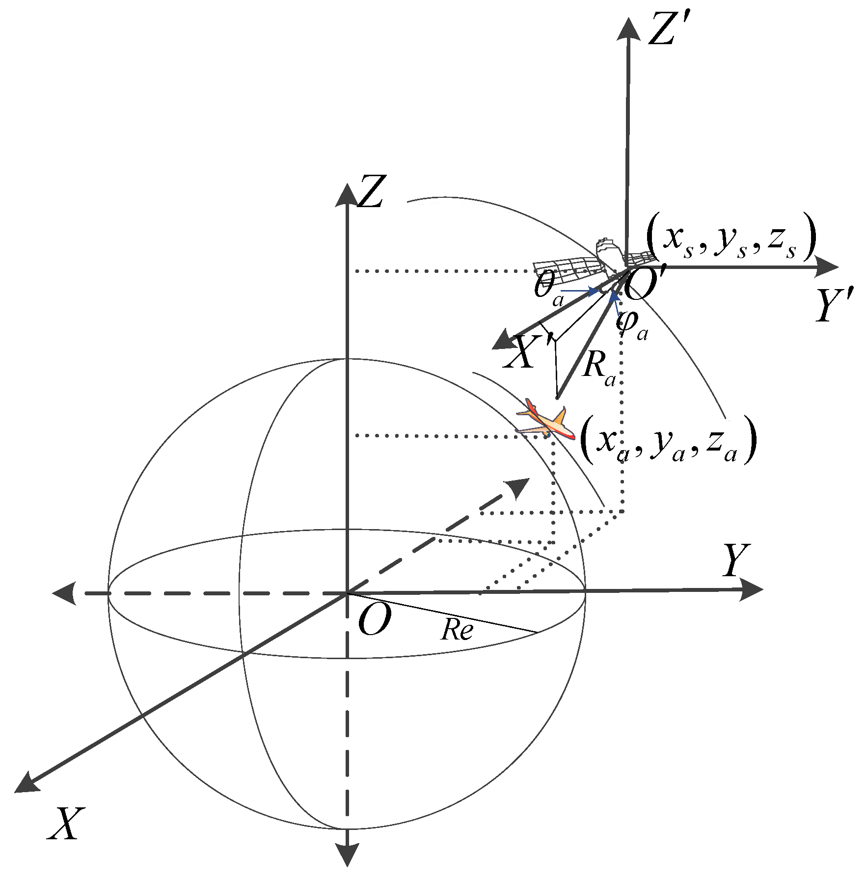
The remainder of this paper is organized as follows. Section 2 establishes the space-based radar observation geometry and the extended target state model. Section 3 presents the extension of the GGIW-PHD filter to three-dimensional space and the implementation of nonlinear filtering with a third-order spherical–radial cubature rule. In Section 4, we derive the recursive formulation of GGIW-PHD-VB processing for both Gaussian and Student’s t-distribution noise models. Section 5 provides an analysis of the simulation results. Finally, Section 6 discusses the findings and potential future work, while Section 7 concludes the paper.

2. Tracking Model of Aerial Extended Targets

2.1. Observation Geometry Model of Space-Based Radar

The radar target tracking model is typically characterized by a state equation and an observation equation. For space-based radar systems, these equations exist in different coordinate systems with a strongly nonlinear transformation relationship. The target state equation is formulated in the Earth-Centered and Earth-Fixed (ECEF) rectangular coordinate system, with the coordinate origin $O$ at the center of the Earth, the $XOY$ plane at the equatorial plane, the $X$-axis pointing to the Greenwich meridian, and the $Z$-axis pointing to the North Pole. The observation equation describes real-time target measurements in the radar body coordinate system, which is parallel to the ECEF coordinate system, and the origin $O^{\prime }$ is the radar’s geometric center.

As shown in Figure 1, in the ECEF rectangular coordinate system, the position of the satellite is $\left(x_s,y_s,z_s\right)$, and that of the aircraft target is $\left(x_a,y_a,z_a\right)$. In the space-based radar coordinate system, the measured value of the aircraft target is $\left(R_a,{\theta }_a,{\phi }_a\right)$, where $R_a$ is the range, ${\theta }_a$ is the azimuth angle, and ${\phi }_a$ is the elevation angle. Then, the conversion relationship between the measurement of the radar coordinate system and the state of the ECEF coordinate system is

$$\begin{array}{l}{x}_a=R_a\cos {\theta }_a\cos {\phi }_a+x_s\\ y_a=R_a\sin {\theta }_a\cos {\phi }_a+y_s\\ z_a=R_a\sin {\phi }_a+z_s\end{array}.$$

(1)

Otherwise,

$$\begin{array}{l}{R}_a=\sqrt{{\left(x_a-x_s\right)}^2+{\left(y_a-y_s\right)}^2+{\left(z_a-z_s\right)}^2}\\ {\theta }_a=\arctan \left[\left(y_a-y_s\right)/\left(x_a-x_s\right)\right]\\ {\phi }_a=\arctan \left[\left(z_a-z_s\right)/\sqrt{{\left(x_a-x_s\right)}^2+{\left(y_a-y_s\right)}^2}\right]\end{array}.$$

(2)

It can be seen from (1) and (2) that the coordinate transformation relationship is strongly nonlinear.

2.2. State Model of Extended Targets

The target extension can be modeled using symmetric, positive-definite random matrices, the statistical properties of which are described by matrix-variate probability densities [8]. The extended target state consists of three parts—the kinematic state, extension state, and measurement rate—formally defined as follows:

$${\xi }_k\triangleq \left({\gamma }_k,x_k,X_k\right).$$

(3)

Here, the random vector ${\mathit{x}}_k={[x_k {\dot{x}}_k y_k {\dot{y}}_k z_k {\dot{z}}_k]}^T$ is the kinematic state. $x_{k,i}$, $y_{k,i}$, and $z_{k,i}$ denote the position and ${\dot{x}}_{k,i}$, ${\dot{y}}_{k,i}$, and ${\dot{z}}_{k,i}$ denote the velocity. The random matrix $X_k\in {\mathbb{S}}_{++}^d$ is the extension state and describes the target’s size and shape. Under the random matrix model, the target shape is assumed to be an ellipsoid. The measurement rate ${\gamma }_k$ is a positive random variable characterizing the expected number of detections generated by the target per observation interval.

Conditioned on a history of previous measurement sets $Z^k$, the extended target state ${\xi }_k$ can be modeled as a GGIW distribution:

$$\begin{gathered} p\left({\xi }_k|Z^k\right)=p\left({\gamma }_k|Z^k\right)p\left(x_k|Z^k\right)p\left(X_k|Z^k\right) \\ \hspace{1em}\hspace{1em}\hspace{1em}\hspace{1em}\hspace{1em}\hspace{1em}\hspace{1em}\hspace{1em}\hspace{1em}\hspace{1em} =𝒢\left({\gamma }_k;{\alpha }_k,{\beta }_k\right)𝒩\left(x_k;m_k,P_k\right)\mathcal{I}{𝒲}_d\left(X_k;v_k,V_k\right), \\ \triangleq 𝒢𝒢\mathcal{I}𝒲\left({\xi }_k;{\zeta }_k\right) \end{gathered}$$

(4)

where ${\zeta }_k=\left\{{\alpha }_k,{\beta }_k,m_k,P_k,v_k,V_k\right\}$ is the set of GGIW distribution parameters. $𝒢$(γ_k;α_k;β_k) denotes a gamma probability density function (PDF) defined over measurement rate ${\gamma }_k$ with scalar shape parameter ${\alpha }_k$ and scalar inverse scale parameter ${\beta }_k$. $𝒩$(x_k;m_k;P_k) denotes the PDF of a Gaussian distribution defined over kinematic state $x_k$, with expected value vector $m_k$ and covariance matrix P_k. $\mathcal{I}{𝒲}_d\left(X_k;v_k,V_k\right)$ denotes an inverse Wishart PDF defined over random matrix $X_k$ with scalar degrees of freedom $v_k$ and parameter matrix $V_k$.

The dynamic motion models describe how the extended target state evolves over time. All targets in the surveillance area are assumed to follow the same dynamic motion model, expressed as follows:

$$x_k=f\left(x_{k-1}\right)+q_{k-1},$$

(5)

where $q_{k-1}$ is Gaussian process noise with zero mean and covariance $Q_{k-1}$, and the motion model $f\left(·\right)$ is generally described as constant velocity, constant acceleration, or coordinated turn model.

The measurement set at time $k$ is the union of a set of clutter detections and a set of target-generated detections, denoted by

$$Z_k=Z_k^{FA}\cup \left(\underset{i=1}{\overset{N_{x,k}}{\cup }}{Z}_k^{\left(i\right)}\right),$$

(6)

where $N_{x,k}$ is the number of true targets. The number of clutter detections is modeled as being Poisson-distributed with measurement rate ${\lambda }_k$, and each clutter detection is modeled as being independently uniformly distributed in the surveillance area. The likelihood of target detections can be modeled as

$$p\left(z_k^{(j)}|{\xi }_k\right)=p\left(z_k^{\left(j\right)}|x_k,X_k\right)=𝒩\left(z_k^{\left(j\right)};h\left(x_k\right),r_k\right),$$

(7)

where $z_k^{(j)}={\left[\begin{array}{ccc}{R}_a& {\theta }_a& {\phi }_a\end{array}\right]}^T$, $j=1,2,\cdots ,N_{z,k}$, and $N_{z,k}$ is the number of target detections. $h\left(·\right)$ is the nonlinear observation model, and the transformation relationship with the state vector can be calculated from (2). $r_k$ is the measurement noise with covariance $R_k$, which can be described as Gaussian or non-Gaussian distributions. The effective detection probability is described as follows:

$$P_{k,D}^e\left({\xi }_k^{\left(i\right)}\right)=\left(1-e^{-{\gamma }_k^{\left(i\right)}}\right)P_D,$$

(8)

where the set of target detections is nonempty with probability $1-e^{-{\gamma }_k^{\left(i\right)}}$, and the set is detected with probability $P_D\in \left[0,1\right]$.

3. GGIW-PHD Nonlinear Filtering for Space-Based Observations

For the GGIW-PHD filter, the extended target state and target motion can be estimated jointly. The random matrix model is used to describe the extended target shape, providing a balance between an informative shape representation and low computational complexity. However, in space-based radar three-dimensional observation scenarios, as shown in (2), the observation model exhibits strong nonlinearity. In [16], a spherical–radial cubature rule was proposed to address high-dimensional nonlinear filtering problems, offering higher approximation accuracy than the extended Kalman filter and unscented Kalman filter. Therefore, in this section, the cubature Kalman filter (CKF) is incorporated into the GGIW-PHD recursions to handle strongly nonlinear models, and the recursive process is implemented using the third-order spherical–radial cubature rule. We denote this as GGIW-PHD-CKF. The detailed recursive procedure is described below.

The PHD $D_k\left(\cdot \right)$ is an intensity function whose integral is the expected value of the number of targets and whose peaks correspond to likely target locations. For extended targets, the PHD intensity $D_k\left(\cdot \right)$ at time $t_k$, given the measurements sets up to and including time $t_k$, is approximated via a mixture of GGIW distributions:

$$D_k\left({\xi }_k\right)={\displaystyle \mathit{\sum }_{j=1}^{J_k}{w}_k^{\left(j\right)}𝒢𝒢\mathcal{I}𝒲\left({\xi }_k;{\zeta }_k^{\left(j\right)}\right)},$$

(9)

where $J_k$ is the number of components, $w_k^{\left(j\right)}$ is the weight of the $j$-th component, and ${\zeta }_k^{\left(j\right)}$ is the density parameter of the $j$-th component.

• Prediction

Assuming that the prior PHD intensity is in the form of (9), the predicted PHD intensity can be expressed as a GGIW mixture with two parts:

$$D_{k|k-1}\left({\xi }_k\right)=D_k^b\left({\xi }_k\right)+D_{k|k-1}^s\left({\xi }_k\right),$$

(10)

where $D_k^b\left(·\right)$ corresponds to new targets appearing in the surveillance area and $D_{k|k-1}^s\left(·\right)$ corresponds to targets that persist in the surveillance area. The probability of a target persisting in the surveillance area is modeled by the survival probability $P_S$. The birth measurement rate and extension are modeled using gamma and inverse Wishart distributions, respectively, while the velocity and acceleration are modeled using Gaussian distributions.

The PHD intensity $D_{k|k-1}^s\left(·\right)$ for existing targets that remain in the surveillance area is

$$D_{k|k-1}^s\left({\xi }_k\right)={\displaystyle \mathit{\sum }_{j=1}^{J_{k|k}}{w}_{k|k-1}^{\left(j\right)}𝒢𝒢\mathcal{I}𝒲\left({\xi }_k;{\zeta }_{k|k-1}^{\left(j\right)}\right)},$$

(11)

where

$$w_{k|k-1}^{\left(j\right)}=P_S{w}_{k-1|k-1}^{\left(j\right)}.$$

(12)

The GGIW distribution parameters of ${\zeta }_{k|k-1}^{\left(j\right)}$ are expressed as

$${\alpha }_{k|k-1}^{\left(j\right)}={\displaystyle \frac{{\alpha }_{k-1|k-1}^{\left(j\right)}}{{\eta }_{k-1}}}, {\beta }_{k|k-1}^{\left(j\right)}={\displaystyle \frac{{\beta }_{k-1|k-1}^{\left(j\right)}}{{\eta }_{k-1}}},$$

(13)

$$v_{k|k-1}^{\left(j\right)}=2d+2+e^{-T_s/\tau }\left(v_{k-1|k-1}^{\left(j\right)}-2d-2\right),$$

(14)

$$V_{k|k-1}^{\left(j\right)}=\left(v_{k|k-1}^{\left(j\right)}-2d-2\right){\left(v_{k-1|k-1}^{\left(j\right)}-2d-2\right)}^{-1},$$

(15)

where $T_s$ is the sampling time, $\tau$ is the temporal decay, ${\eta }_{k-1}$ is the forgetting factor, and $d$ is the dimension of the random matrix $X_k$ that describes the target’s size and shape. Additionally, for each Gaussian component characterized by mean $m_{k-1}^{\left(j\right)}$ and covariance $P_{k-1}^{\left(j\right)}$, the predicted mean $m_{k|k-1}^{\left(j\right)}$ and covariance matrix $P_{k|k-1}^{\left(j\right)}$ are calculated through the following steps:

(i)

Given $P_{k-1}^{\left(j\right)}$, using Cholesky decomposition, we can obtain $P_{k-1}^{\left(j\right)}=S_{k-1}^{\left(j\right)}{\left(S_{k-1}^{\left(j\right)}\right)}^T$;

(ii)

According to the dimension $n_x$ of the target state vector $x_{k-1}$, the number of cubature points is determined as $u=2n_x$. Then, the cubature points ${\chi }_{p,k-1}$, for $p=1,2,\dots ,u$, can be generated from $m_{k-1}^{\left(j\right)}$ and $S_{k-1}^{\left(j\right)}$ based on the following equation:

$${\chi }_{p,k-1}=S_{k-1}^{\left(j\right)}{\varsigma }_p+m_{k-1}^{(j)},$$

(16)

where ${\varsigma }_p=\sqrt{u/2}{\left[\mathbf{1}\right]}_p$, $\left[\mathbf{1}\right]=\left[1\times I_{n_x},-1\times I_{n_x}\right]$, $I_{n_x}\in {ℝ}^{n_x}$ is an identity matrix, and ${\left[\mathbf{1}\right]}_p$ represents the $p$-th column of $\left[\mathbf{1}\right]$.

(iii)

The propagated cubature points are calculated according to the nonlinear motion model equation for a single target:

$${\chi }_{p,k|k-1}=f_{k|k-1}\left({\chi }_{p,k-1}\right),p=1,2,\dots ,u.$$

(17)

(iv)

The predicted mean and covariance are expressed as

$$m_{k|k-1}^{(j)}={\displaystyle \frac{1}{u}}{\displaystyle \mathit{\sum }_{p=1}^u{\chi }_{p,k|k-1}},$$

(18)

$$P_{k|k-1}^{(j)}={\displaystyle \mathit{\sum }_{p=1}^u{\chi }_{p,k|k-1}{\left({\chi }_{p,k|k-1}\right)}^T}-m_{k|k-1}^{(j)}{\left(m_{k|k-1}^{(j)}\right)}^T+Q_k.$$

(19)

• Update

The measurement updated PHD intensity based on the measurements up to time $k$ can be expressed as

$$D_k\left({\xi }_k|Z^k\right)=L_{Z_k}\left({\xi }_k\right)D_{k|k-1}\left({\xi }_k|Z^{k-1}\right),$$

(20)

where $L_{Z_k}\left({\xi }_k\right)$ is the measurement pseudolikelihood, derived as follows:

$$L_{Z_k}\left({\xi }_k\right)\triangleq 1-P_{k,D}^e+e^{-{\gamma }_k}{P}_D{\displaystyle \mathit{\sum }_{𝒫\angle Z_k}{\omega }_{𝒫}{\displaystyle \mathit{\sum }_{W\in 𝒫}\frac{{\gamma }_k^{\left|W\right|}}{d_W}}{\displaystyle \mathbf{\prod }_{z_k\in W}\frac{{\varphi }_{z_k}\left({\xi }_k\right)}{{\lambda }_k{c}_k\left(z_k\right)}}}.$$

(21)

The first part corresponds to missed detections, and the second part corresponds to detected targets. Here, $P_{k,D}^e$ is the effective probability of detection; ${\lambda }_k$ is the average number of clutter returns per unit volume; $c_k\left(\cdot \right)$ is the spatial distribution of the clutter over the surveillance volume; ${\varphi }_{z_k}\left({\xi }_k\right)$ is the likelihood function for a single target-generated measurement; and $𝒫\angle Z_k$ represents that $𝒫$ partitions the measurement set Z_k into non-empty cells W. As the size of the measurement set increases, the number of possible partitions grows very large. We adopt the density-based spatial clustering of applications with noise (DBSCAN) method [17] to partition the measurement clusters. As a density-based clustering algorithm, DBSCAN starts with a randomly selected sample point and iteratively explores neighboring points within a specified radius until all samples are processed. This approach effectively identifies clusters of arbitrary shapes in noisy datasets.

The terms ω_$𝒫$ and $d_W$ represent non-negative coefficients defined for each partition $𝒫$ and cell $W$, respectively, as follows:

$${\omega }_{𝒫}={\displaystyle \frac{{\displaystyle {\prod }_{W\in 𝒫}{d}_W}}{{\displaystyle {\mathit{\sum }}_{𝒫\prime \angle Z_k}{\displaystyle {\prod }_{W^{\prime }\in {𝒫}^{\prime }}{d}_{W^{\prime }}}}}},$$

(22)

$$d_W={\delta }_{\left|W\right|,1}+D_{k|k-1}\left[P_D{\gamma }_k^{\left|W\right|}{e}^{-{\gamma }_k}{\displaystyle \prod _{z_k\in W}\frac{{\varphi }_{z_k}\left(\cdot \right)}{{\lambda }_k{c}_k\left(z_k\right)}}\right].$$

(23)

Then, the posterior PHD $D_k\left({\xi }_k\right)$ can be denoted as a GGIW mixture form with three parts corresponding to previously existing targets that are not detected, new targets, and previously existing targets that continue to be detected:

$$D_k\left({\xi }_k\right)=D_k^b\left({\xi }_k\right)+D_k^m\left({\xi }_k\right)+D_k^d\left({\xi }_k\right).$$

(24)

(i)

The PHD corresponding to new targets is

$$D_k^b\left({\xi }_k\right)={\displaystyle \mathit{\sum }_{𝒫\angle Z_k}{\displaystyle \mathit{\sum }_{W\in 𝒫}{w}_k^{\left(b,W\right)}𝒢𝒢\mathcal{I}𝒲\left({\xi }_k;{\zeta }_k^{\left(b,W\right)}\right).}}$$

(25)

(ii)

The updated PHD corresponding to previously existing targets that are not detected is as follows:

$$\begin{array}{l}{D}_k^m\left({\xi }_k\right)={\displaystyle \mathit{\sum }_{j=1}^{J_{k|k-1}}\left(1-P_{k,D}^e\right)w_{k|k-1}^{\left(j\right)}𝒢𝒢\mathcal{I}𝒲\left({\xi }_k;{\tilde{\zeta }}_{k|k-1}^{\left(j\right)}\right)}\\ ={\displaystyle \mathit{\sum }_{j=1}^{J_{k|k-1}}{\tilde{w}}_k^{\left(j\right)}𝒢𝒢\mathcal{I}𝒲\left({\xi }_k;{\tilde{\zeta }}_{k|k}^{\left(j\right)}\right)}\end{array},$$

(26)

where ${\tilde{\zeta }}_{k|k}^{\left(j\right)}=\left\{{\tilde{\alpha }}_k^{\left(j\right)},{\tilde{\beta }}_k^{\left(j\right)},m_{k|k-1}^{\left(j\right)},P_{k|k-1}^{\left(j\right)},v_{k|k-1}^{\left(j\right)},V_{k|k-1}^{\left(j\right)}\right\}$.

(iii)

The PHD corresponding to previously existing targets that continue to be detected is updated according to the measurement model (7), and the detailed process is described as follows:

$$D_k^d\left({\xi }_k\right)={\displaystyle \mathit{\sum }_{𝒫\angle Z_k}{\displaystyle \mathit{\sum }_{W\in 𝒫}{\displaystyle \mathit{\sum }_{j=1}^{J_{k|k-1}}{w}_k^{\left(j,W\right)}𝒢𝒢\mathcal{I}𝒲\left({\xi }_k;{\zeta }_k^{\left(j,W\right)}\right)}}},$$

(27)

where the GGIW distribution parameters of ${\zeta }_k^{\left(j,W\right)}$ are expressed as

$${\alpha }_k^{\left(j,W\right)}={\alpha }_{k|k-1}^{\left(j\right)}+\left|W\right|,$$

(28)

$${\beta }_k^{\left(j,W\right)}={\beta }_{k|k-1}^{\left(j\right)}+1,$$

(29)

$$v_k^{\left(j,W\right)}=v_{k|k-1}^{\left(j,W\right)}+\left|W\right|,$$

(30)

$$V_k^{\left(j,W\right)}=V_{k|k-1}^{\left(j\right)}+N_{k|k-1}^{\left(j,W\right)}+Z_{k|k-1}^{\left(j,W\right)}.$$

(31)

The centroid measurement of cell $W$ is

$${\overline{z}}_k^{\left(j,W\right)}={\displaystyle \frac{1}{\left|W\right|}}{\displaystyle \mathit{\sum }_{z_k^{\left(i\right)}\in W}{z}_k^{\left(i\right)}}.$$

(32)

Then, we obtain

$$Z_k^{\left(j,W\right)}={\displaystyle \mathit{\sum }_{z_k^{\left(i\right)}\in W}\left(z_k^{\left(i\right)}-{\overline{z}}_k^{\left(j,W\right)}\right){\left(z_k^{\left(i\right)}-{\overline{z}}_k^{\left(j,W\right)}\right)}^T},$$

(33)

$${\epsilon }_{k|k-1}^{\left(j,W\right)}={\overline{z}}_k^{\left(j,W\right)}-h_k\left(m_{k|k-1}^{\left(j\right)}\right),$$

(34)

$$N_{k|k-1}^{\left(j,W\right)}={\left(S_{k|k-1}^{\left(\mathrm{j},W\right)}\right)}^{-1}{\epsilon }_{k|k-1}^{\left(\mathrm{j},W\right)}{\left({\epsilon }_{k|k-1}^{\left(\mathrm{j},W\right)}\right)}^T.$$

(35)

Given the predicted mean $m_{k|k-1}^{(j,W)}$ and predicted covariance matrix $P_{k|k-1}^{(j,W)}$, the measurement update can be calculated as follows:

(i)

The prediction of cubature points is expressed as

$${\chi }_{p,k|k-1}=S_{k|k-1}^{(j,W)}{\varsigma }_p+m_{k|k-1}^{(j,W)}, p=1,2,\dots ,u.$$

(36)

(ii)

The propagated cubature points are calculated via the observational model:

$${\mathcal{Z}}_{p,k|k-1}=h_k\left({\chi }_{p,k|k-1}\right), p=1,2,\dots ,u.$$

(37)

(iii)

The predicted measurement is estimated as follows:

$$z_{k|k-1}^{(j,W)}={\displaystyle \frac{1}{u}}{\displaystyle \mathit{\sum }_{p=1}^u{\mathcal{Z}}_{p,k|k-1}}.$$

(38)

(iv)

The state-measurement cross-covariance matrix is estimated as follows:

$$P_{(xz)k|k-1}^{(j,W)}={\displaystyle \frac{1}{u}}{\displaystyle \mathit{\sum }_{p=1}^u{\chi }_{p,k|k-1}{\mathcal{Z}}_{p,k|k-1}}-m_{k|k-1}^{(j,W)}{\left(z_{k|k-1}^{(j,W)}\right)}^T.$$

(39)

(v)

The measurement innovation covariance matrix is estimated as follows:

$$P_{\left(zz\right)k|k-1}^{(j,W)}={\displaystyle \frac{1}{u}}{\displaystyle \mathit{\sum }_{p=1}^u{\mathcal{Z}}_{p,k|k-1}{\left({\mathcal{Z}}_{p,k|k-1}\right)}^T}-z_{k|k-1}^{(j,W)}{\left(z_{k|k-1}^{(j,W)}\right)}^T+R_k^{\left(j\right)}.$$

(40)

The state update is calculated as follows:

$$m_k^{(j,W)}=m_{k|k-1}^{(j,W)}+K_k^{\left(j,W\right)}\left(z_k^{(j,W)}-z_{k|k-1}^{(j,W)}\right),$$

(41)

$$K_k^{\left(j,W\right)}=P_{(xz)k|k-1}^{(j,W)}{\left(P_{\left(zz\right)k|k-1}^{(j,W)}\right)}^{-1},$$

(42)

$$P_k^{(j,W)}=P_{k|k-1}^{(j,W)}-K_k^{\left(j,W\right)}{P}_{\left(zz\right)k|k-1}^{(j,W)}{\left(K_k^{\left(j,W\right)}\right)}^{-1}.$$

(43)

Then, $S_k^{\left(j,W\right)}$ is obtained via the Cholesky decomposition of $P_k^{(j,W)}$, i.e., $P_k^{(j,W)}=S_k^{\left(j,W\right)}{\left(S_k^{\left(j,W\right)}\right)}^T$.

The updated GGIW component weight is given by

$$w_{k|k}^{\left(j,W\right)}={\displaystyle \frac{{\omega }_{𝒫}}{d_W}}{e}^{-{\gamma }^{\left(j\right)}}{\left({\displaystyle \frac{{\gamma }^{\left(j\right)}}{{\beta }_{FA,k}}}\right)}^{\left|W\right|}{P}_D^{\left(j\right)}{L}_k^{\left(j,W\right)}{w}_{k|k-1}^{\left(j\right)},$$

(44)

where $L_k^{\left(j,W\right)}$ is the measurement likelihood expressed as follows:

$$L_k^{\left(j,W\right)}={\displaystyle \frac{1}{{\left({\pi }^{\left|W\right|}\left|W\right|S_{k|k-1}^{\left(j,W\right)}\right)}^{\frac{d}{2}}}}{\displaystyle \frac{{\left|V_{k|k-1}^{\left(j\right)}\right|}^{\frac{v_{k|k-1}^{\left(j\right)}}{2}}}{{\left|V_k^{\left(j,W\right)}\right|}^{\frac{v_k^{\left(j,W\right)}}{2}}}}{\displaystyle \frac{{\Gamma }_d\left(\frac{v_k^{\left(j,W\right)}}{2}\right)}{{\Gamma }_d\left(\frac{v_{k|k-1}^{\left(j\right)}}{2}\right)}},$$

(45)

$$d_W={\delta }_{\left|W\right|,1}+{{\displaystyle \mathit{\sum }_{l=1}^{J_{k|k-1}}{e}^{-{\gamma }^{\left(l\right)}}\left(\frac{{\gamma }^{\left(l\right)}}{{\beta }_{FA,k}}\right)}}^{\left|W\right|}{P}_D^{\left(l\right)}{L}_k^{\left(l,W\right)}{w}_{k|k-1}^{\left(l\right)}.$$

(46)

4. GGIW-PHD Nonlinear Filtering with VB Processing for Uncertain Measurement Noise Parameters

For space-based radar target tracking, challenges such as high-speed platform movement, long-range detection, perturbation interference, and nonlinear observations may cause the measurement noise to exhibit anomalous non-Gaussian and heavy-tailed distributions. To address this, we model the measurement noise using both Gaussian and non-Gaussian representations. Furthermore, we enhance the GGIW-PHD-CKF by incorporating VB processing [18], with the enhanced filter denoted by GGIW-PHD-CKF-VB, thereby improving tracking robustness in complex noise environments.

4.1. Measurement Noise with Gaussian Distribution

4.1.1. Measurement Noise Parameter Model

Assume that the measurement noise $r_k$ is zero-mean Gaussian white noise with covariance matrix $R_k$. Since the inverse gamma distribution serves as the conjugate prior for the covariance of the Gaussian distribution, the posterior distribution of $R_k$ can be approximated as a product of independent inverse gamma distributions:

$$q\left(R_k\right)\approx {\displaystyle \prod _{l=1}^m\mathcal{I}𝒢\left({\sigma }_{k,l};a_{k,l},b_{k,l}\right)},$$

(47)

where $\mathcal{I}𝒢\left({\sigma }_{k,l};a_{k,l},b_{k,l}\right)$ denotes an inverse gamma distribution, $m$ is the dimension, $a$ is the shape parameter, and $b$ is the scale parameter, i.e.,

$$\mathcal{I}𝒢\left(\sigma ;a,b\right)={\displaystyle \frac{b^a}{\Gamma \left(a\right)}}{\sigma }^{-a-1}\exp \left(-{\displaystyle \frac{b}{a}}\right),$$

(48)

where

$$\Gamma \left(a\right)={\displaystyle {\int }_0^{\infty }{t}^{a-1}\exp \left(-t\right)dt}.$$

(49)

4.1.2. Variational Bayesian Approximation

Assume that the dynamic models of the target state and measurement noise variances are independent, i.e.,

$$f_{k|k-1}\left(x_k,R_k|x_{k-1},R_{k-1}\right)=f_{k|k-1}\left(x_k|x_{k-1}\right)f_{k|k-1}\left(R_k|R_{k-1}\right).$$

(50)

The predictive distribution is given by the Chapman–Kolmogorov equation:

$$\begin{array}{l}{p}_{k|k-1}\left(x_k,R_k|Z_{1:k-1}\right)={\displaystyle \int f_{k|k-1}\left(x_k|x_{k-1}\right)f_{k|k-1}\left(R_k|R_{k-1}\right)}\\ \times p_{k-1}\left(x_{k-1},R_{k-1}|Z_{1:k-1}\right)dxdR\end{array}.$$

(51)

The updated posterior distribution is derived by applying the Bayes rule:

$$p_k\left(x_k,R_k|Z_{1:k}\right)={\displaystyle \frac{g_k\left(Z_k|x_k,R_k\right)p_{k|k-1}\left(x_k,R_k|Z_{1:k-1}\right)}{{\displaystyle \int g_k\left(Z_k|x_k,R_k\right)p_{k|k-1}\left(x_k,R_k|Z_{1:k-1}\right)dxdR}}}.$$

(52)

Since the target state and the measurement noise covariance matrix are coupled in the likelihood function $p_k\left(x_k,R_k|Z_{1:k}\right)$, the analytical form of the posterior distribution is difficult to derive. With the introduction of the VB approximation, the posterior distribution can be approximately decomposed into

$$p_k\left(x_k,R_k|Z_{1:k}\right)\approx Q_x\left(x_k\right)Q_R\left(R_k\right),$$

(53)

where the approximated posterior densities can be determined by minimizing the Kullback–Leibler (KL) divergence between the separable approximation and the true posterior density [18]:

$$\begin{array}{l}KL\left[Q_x\left(x_k\right)Q_R\left(R_k\right)\left|\right|p_k\left(x_k,R_k|Z_{1:k}\right)\right]={\displaystyle \int Q_x\left(x_k\right)Q_R\left(R_k\right)}\\ \times \log \left({\displaystyle \frac{Q_x\left(x_k\right)Q_R\left(R_k\right)}{p_k\left(x_k,R_k|Z_{1:k}\right)}}\right)dxdR\end{array}.$$

(54)

The optimization problem can be resolved by optimizing with respect to $Q_x\left(x_k\right)$ and $Q_R\left(R_k\right)$ sequentially while keeping the other fixed. Then, the approximated posterior densities are

$$Q_x\left(x_k\right)=𝒩\left(x_k;m_k,P_k\right),$$

(55)

$$Q_R\left(R_k\right)={\displaystyle \prod _{l=1}^m\mathcal{I}𝒢\left({\sigma }_{k,l};a_{k,l},b_{k,l}\right)}.$$

(56)

4.1.3. GGIW-PHD-CKF-VB Filter Implementation

The recursive framework of GGIW-PHD nonlinear filtering for space-based three-dimensional observation scenarios was developed in Section 3. With the introduction of VB processing, the modified recursive procedure is formally derived as follows:

• Prediction

The predicted intensity of survival targets is expressed as

$$D_{k|k-1}^s\left({\xi }_k,R_k\right)={\displaystyle \mathit{\sum }_{j=1}^{J_{k-1}}{w}_{k|k-1}^{\left(j\right)}𝒢𝒢\mathcal{I}𝒲\left({\xi }_k;{\zeta }_{k|k-1}^{\left(j\right)}\right)\times {\displaystyle \prod _{l=1}^m\mathcal{I}𝒢\left({\left({\sigma }_{k,l}^{\left(j\right)}\right)}^2;a_{k|k-1,l}^{\left(j\right)},b_{k|k-1,l}^{\left(j\right)}\right)}},$$

(57)

and the predicted measurement noise parameters are

$$a_{k|k-1,l}^{\left(j\right)}={\rho }_l{a}_{k,l}^{\left(j\right)},$$

(58)

$$b_{k|k-1,l}^{\left(j\right)}={\rho }_l{b}_{k,l}^{\left(j\right)},$$

where ${\rho }_l\in \left(0,1\right]$ is the degradation factor. The calculations for the other parameters are consistent with those for the GGIW-PHD filter. The weight of the j-th component, $w_{k|k-1}^{\left(j\right)}$, is shown in (12). For the GGIW distribution parameters in ${\zeta }_{k|k-1}^{\left(j\right)}$, the measurement rate distribution parameters ${\alpha }_{k|k-1}^{\left(j\right)}$ and ${\beta }_{k|k-1}^{\left(j\right)}$ are shown in (13). The random matrix parameters $v_{k|k-1}^{\left(j\right)}$ and $V_{k|k-1}^{\left(j\right)}$ are shown in (14) and (15). The mean $m_{k|k-1}^{(j)}$ and covariance $P_{k|k-1}^{(j)}$ of the Gaussian component are shown in (18) and (19).

• Update

For the posterior PHD, denoted as a GGIW mixture form in (24), the previously existing targets that continue to be detected are updated as follows:

$$D_{k|k}^d\left({\xi }_k,R_k\right)={\displaystyle \mathit{\sum }_{𝒫\angle Z_k}{\displaystyle \mathit{\sum }_{W\in 𝒫}{\displaystyle \mathit{\sum }_{j=1}^{J_k}{w}_{k|k}^{\left(j,W\right)}𝒢𝒢\mathcal{I}𝒲\left({\xi }_k;{\zeta }_{k|k}^{\left(j,W\right)}\right)\times {\displaystyle \prod _{l=1}^m\mathcal{I}𝒢\left({\left({\sigma }_{k|k}^{\left(j\right)}\right)}^2;a_{k,l}^{\left(j\right)},b_{k,l}^{\left(j\right)}\right)}}}},$$

(59)

where

$$a_{k,l}^{\left(j,0\right)}={\displaystyle \frac{1}{2}}+a_{k|k-1,l}^{\left(j\right)},$$

(60)

$$b_{k,l}^{\left(j,0\right)}=b_{k|k-1,l}^{\left(j\right)}.$$

For each cell $W$, the parameters of the $n$-th iteration are

$$R_k^{\left(j,W\right)\left(n\right)}=diag\left(\left[{\displaystyle \frac{b_{k,1}^{\left(j\right)\left(n\right)}}{a_{k,1}^{\left(j\right)\left(n\right)}}},\cdots ,{\displaystyle \frac{b_{k,m}^{\left(j\right)\left(n\right)}}{a_{k,m}^{\left(j\right)\left(n\right)}}}\right]\right),$$

(61)

$$a_{k,l}^{\left(j,n\right)}={\displaystyle \frac{1}{2}}+a_{k,l}^{\left(j,n-1\right)},$$

(62)

$$b_{k,l}^{\left(j\right)\left(n\right)}=b_{k,l}^{\left(j,n-1\right)}+{\displaystyle \frac{1}{2}}{\left(z_k-z_{k|k-1}^{(j)}\right)}_l^2+{\displaystyle \frac{1}{2}}{\left(S_k^{\left(j,W\right)}\right)}_{ll},$$

(63)

where the target state parameters $m_k^{\left(j,W\right)}$, $P_k^{\left(j,W\right)}$, $K_k^{\left(j,W\right)}$, and $S_k^{\left(j,W\right)}$ are calculated and iterated according to Equations (41)–(43) until $‖m_k^{\left(j,W\right)\left(n+1\right)}-m_k^{\left(j,W\right)\left(n\right)}‖\le \epsilon$ for the given threshold ε. The parameters of the measurement rate distribution are updated using (28) and (29), and the random matrix parameters are updated using (30) and (31).

4.2. Measurement Noise with Non-Gaussian Distribution

4.2.1. Measurement Noise Parameter Model

While Gaussian distributions are commonly employed for modeling measurement noise due to their mathematical tractability, they prove inadequate for space-based radar tracking scenarios where target aspect variations induce irregular electromagnetic reflections. These phenomena generate non-Gaussian disturbances, particularly glint noise, characterized by a heavy-tailed distribution [13]. Empirical evidence demonstrates that conventional filtering algorithms exhibit degraded performance under such conditions. Student’s t-distribution demonstrates superior robustness to outliers when compared to Gaussian models, but its adoption introduces significant analytical challenges. To address these limitations, VB methods have been employed to derive tractable approximate distributions.

In this section, the measurement noise r_k in (7) is described using a heavy-tailed m-dimensional Student’s t-distribution:

$$p_z\left(z_k|h\left(x_k\right),R_k,u_k\right)=S\left(z_k;h\left(x_k\right),R_k,u_k\right),$$

(64)

where $S\left(z;\overline{z},\mathit{\Sigma },v\right)$ denotes the probability density function of Student’s t-distribution with mean $\overline{z}$, precision $\mathit{\Sigma }$, and degree of freedom $v$. The probability density function is

$$\begin{array}{l}S\left(z;\overline{z},\mathit{\Sigma },v\right)={\displaystyle \frac{\Gamma \left(\frac{m+v}{2}\right)}{\Gamma \left(\frac{v}{2}\right){\left(\pi v\right)}^{\frac{m}{2}}}}{\left|\mathit{\Sigma }\right|}^{{\displaystyle \frac{1}{2}}}{\left[1+{\displaystyle \frac{{\left(z-\overline{z}\right)}^T\mathit{\Sigma }\left(z-\overline{z}\right)}{v}}\right]}^{-{\displaystyle \frac{m+v}{2}}}\\ ={\displaystyle {\int }_0^{\infty }𝒩\left(z;\overline{z},{\left(s\mathit{\Sigma }\right)}^{-1}\right)\times 𝒢\left(s;\frac{v}{2},\frac{v}{2}\right)}\end{array},$$

(65)

where $\Gamma \left(a\right)={\displaystyle {\int }_0^{\infty }{u}^{a-1}{e}^{-u}du}$ is the gamma function. $𝒢$(s;κ;θ) = (θ^κ/Γ(κ))s^κ−1e^−θs is the probability density function of a Gamma distribution in terms of shape parameter $\kappa$ and inverse scale parameter $\theta$.

4.2.2. Variational Bayesian Approximation

The posterior probability density of multi-target Bayesian prediction and update is described as

$$\begin{array}{l}{p}_{k|k-1}\left(x_k,R_k,u_k|Z_{1:k-1}\right)={\displaystyle \int f_{k|k-1}\left(x_k,R_k,u_k|x_{k-1},R_{k-1},u_k\right)}\\ \times p_{k-1}\left(x_{k-1},R_{k-1},u_k|Z_{1:k-1}\right)dxdRdu\end{array},$$

(66)

$$p_k\left(x_k,R_k,u_k|Z_{1:k}\right)={\displaystyle \frac{g_k\left(Z_k|x_k,R_k,u_k\right)p_{k|k-1}\left(x_k,R_k,u_k|Z_{1:k-1}\right)}{{\displaystyle \int g_k\left(Z_k|x_k,R_k,u_k\right)p_{k|k-1}\left(x_k,R_k,u_k|Z_{1:k-1}\right)dxdRdu}}}.$$

(67)

With the introduction of the VB approximation, the posterior distribution can be approximately decomposed into

$$p_k\left(x_k,R_k,u_k|Z_{1:k}\right)\approx Q_x\left(x_k\right)Q_R\left(R_k\right)Q_u\left(u_k\right).$$

(68)

The approximated posterior densities can be determined by minimizing the KL divergence between the separable approximation and the true posterior density. Then, the approximated posterior densities are

$$Q_x\left({\mathit{x}}_k\right)=𝒩\left({\mathit{x}}_k;{\mathit{m}}_k,{\mathit{P}}_k\right),$$

(69)

$$Q_R\left(R_k\right)={\displaystyle \prod _{l=1}^m𝒢\left(r_{k,l};a_{k,l},{\mathrm{b}}_{k,l}\right)},$$

(70)

$$Q_u\left(u_k\right)=𝒢\left(u_k;{\gamma }_k,{\eta }_k\right).$$

(71)

4.2.3. GGIW-PHD-CKF-VB Filter Implementation

The recursion process of the GGIW-PHD-CKF-VB filter for measurement noise with Student’s t-distribution is as follows.

• Prediction

The predicted intensity of survival targets is expressed as

$$D_{k|k-1}^s\left({\xi }_k,R_k,u_k\right)={\displaystyle \mathit{\sum }_{j=1}^{J_{k-1}}{\displaystyle \prod _{l=1}^m{w}_{k|k-1}^{\left(j\right)}𝒢𝒢\mathcal{I}𝒲\left({\xi }_k;{\zeta }_{k|k-1}^{\left(j\right)}\right)𝒢\left(r_{k,l};a_{k|k-1,l}^{\left(j\right)},{\mathrm{b}}_{k|k-1,l}^{\left(j\right)}\right)𝒢\left(u_k;{\gamma }_{k|k-1}^{\left(j\right)},{\eta }_{k|k-1}^{\left(j\right)}\right)}},$$

(72)

and the predicted measurement noise parameters are

$$a_{k|k-1,l}={\rho }_{a,l}{a}_{k-1,l},$$

(73)

$$b_{k|k-1,l}={\rho }_{b,l}{b}_{k-1,l},$$

(74)

$${\gamma }_{k|k-1}={\rho }_{\gamma }{\gamma }_{k-1},$$

(75)

$${\eta }_{k|k-1}={\rho }_{\eta }{\eta }_{k-1},$$

(76)

where ${\rho }_{a,l}$, ${\rho }_{\mathrm{b},l}$, ${\rho }_{\gamma }$, and ${\rho }_{\eta }$ are degradation factors with the values in the range of $\left(0,1\right]$. The calculations for the other parameters are consistent with those for the GGIW-PHD filter. The weight $w_{k|k-1}^{\left(j\right)}$ is shown in (12). The measurement rate distribution parameters are shown in (13). The random matrix parameters are shown in (14) and (15), and the mean and covariance of the Gaussian component are shown in (18) and (19).

• Update

For the posterior PHD denoted as a GGIW mixture form in (24), the previously existing targets that continue to be detected are updated as follows:

$$D_{k|k}^d\left({\xi }_k,R_k,u_k\right)={\displaystyle \mathit{\sum }_{𝒫\angle Z_k}{\displaystyle \mathit{\sum }_{W\in 𝒫}{\displaystyle \mathit{\sum }_{j=1}^{J_k}{\displaystyle \prod _{l=1}^m{w}_{k|k}^{\left(j,W\right)}𝒢𝒢\mathcal{I}𝒲\left({\xi }_k;{\zeta }_{k|k}^{\left(j,W\right)}\right)𝒢\left(r_{k,l};a_{k,l}^{\left(j\right)},b_{k,l}^{\left(j\right)}\right)𝒢\left(u_k;{\gamma }_k^{\left(j\right)},{\eta }_k^{\left(j\right)}\right)}}}}.$$

(77)

The parameter update process of $R_k^{\left(j,W\right)}$ is performed via the following steps:

$${\widehat{R}}_k^{\left(j,W\right)}=diag\left\{{\displaystyle \frac{a_{k,1}}{b_{k,1}}},\cdots ,{\displaystyle \frac{a_{k,m}}{b_{k,m}}}\right\},$$

(78)

$$a_{k,l}=0.5+a_{k|k-1,l},$$

(79)

$$b_{k,l}=b_{k|k-1,l}+0.5\times tr\left[{\widehat{s}}_k\left(z_k-z_{k|k-1}^{(j)}\right){\left(z_k-z_{k|k-1}^{(j)}\right)}^T+S_k^{\left(j,W\right)}\right],$$

(80)

$${\gamma }_k=0.5+{\gamma }_{k|k-1},$$

(81)

$${\eta }_k={\eta }_{k|k-1}-{\displaystyle \frac{1}{2}}\left[1+{\Gamma }^{\prime }\left({\alpha }_k\right)/\Gamma \left({\alpha }_k\right)-\log {\beta }_k-{\widehat{s}}_k\right],$$

(82)

$${\alpha }_k={\displaystyle \frac{1}{2}}\left(1+{\gamma }_k/{\eta }_k\right),$$

(83)

$${\beta }_k={\displaystyle \frac{1}{2}}\left({\displaystyle \frac{{\gamma }_k}{{\eta }_k}}+tr\left[{\widehat{R}}_k^{\left(j,W\right)}\left(z_k-z_{k|k-1}^{(j)}\right){\left(z_k-z_{k|k-1}^{(j)}\right)}^T+S_k^{\left(j,W\right)}\right]\right),$$

(84)

$${\widehat{s}}_k={\alpha }_k/{\beta }_k.$$

(85)

The target state parameters $m_k^{\left(j,W\right)}$, $P_k^{\left(j,W\right)}$, $K_k^{\left(j,W\right)}$, and $S_k^{\left(j,W\right)}$ are calculated and iterated according to Equations (41)–(43) until $‖m_k^{\left(j,W\right)\left(n+1\right)}-m_k^{\left(j,W\right)\left(n\right)}‖\le \epsilon$, where $\epsilon$ is the given threshold. The parameters of the measurement rate distribution are updated using (28) and (29), and the random matrix parameters are updated using (30) and (31).

5. Simulation Results

5.1. Simulation Scenario and Parameters

A semi-physical simulation method [19] was adopted to simulate a realistic observation scenario as accurately as possible. We utilized actual orbital data from the Qilu-1 satellite to model the space-based radar motion. Qilu-1 is a synthetic aperture radar (SAR) imaging satellite operating in the Ku-band with an orbital altitude of 500 km. Aircraft target trajectories were sourced from an automatic dependent surveillance broadcast (ADS-B) dataset. By performing temporal and spatial alignment of the satellite and aircraft trajectories, we established a simulated scenario, as depicted in Figure 2a. The spatial positional relationship within the ECEF coordinate system is shown in Figure 2b. On this basis, we added measurement noise in the range, azimuth, and elevation dimensions within the space-based radar observation coordinate system to generate target measurements. Clutter measurements were also added within the observation area; these were modeled as a Poisson RFS $K_k$ with intensity κ_k(z) = λ_cVU(z), where U(•) is the uniform density over the surveillance region, $V$ is the ‘volume’ of the surveillance region, and ${\lambda }_c$ is the average number of clutter returns per unit volume. Since civil aircraft targets generally remain in stable flight phases, a constant velocity motion model was employed in the simulation to characterize their kinematic state transitions. The optimal subpattern assignment (OSPA) metric [20] and root-mean-square error (RMSE) were adopted to evaluate the target tracking performance.

5.2. Performance Analysis of Aerial Extended Target Tracking

For the GGIW-PHD-CKF, the extended target shape is characterized by the random matrix $X_k$ in (4), commonly termed the shape covariance matrix of an ellipsoid. The square roots of its eigenvalues determine the semi-axis lengths of the ellipsoid, while the eigenvectors define the orientations of the principal axes. In this section, we evaluate the tracking performance of the GGIW-PHD-CKF in a space-based radar three-dimensional nonlinear observation scenario by systematically varying the extended target shape parameters. As detailed in

Table 1. The shape parameter settings of extended targets.

Scenario Index	Shape Covariance Matrix	Shape Parameter (m)
		Semi-Axis of X-Direction	Semi-Axis of Y-Direction	Semi-Axis of Z-Direction
1	/	100	100	100
2	$\left[\begin{array}{ccc}42.3& 9.5& 2.2\\ 9.5& 37.3& 1.7\\ 2.2& 1.7& 30.4\end{array}\right]$	30	30	50
3	$\left[\begin{array}{ccc}46.8& 28.5& 6.6\\ 28.5& 32.0& 5.1\\ 6.6& 5.1& 11.2\end{array}\right]$	10	10	70

, three distinct scenarios are considered. Scenario 1 corresponds to a standard spherical shape, and scenarios 2–3 correspond to ellipsoidal configurations with different semi-axis settings.

This section presents a comparative analysis of the tracking performance of the GGIW-PHD-CKF and ET-PHD [9] filters under varying target shape parameters. The conventional ET-PHD filter operates through measurement clustering and weighting for extended target tracking, whereas the proposed GGIW-PHD-CKF incorporates shape parameter estimation, demonstrating enhanced adaptability to targets with diverse shape characteristics. The OSPA distance comparisons in Figure 3 reveal that both filters experience tracking accuracy degradation as the target shape transitions from spherical to oblate ellipsoidal configurations. However, the GGIW-PHD-CKF maintains faster convergence and superior precision throughout these shape variations. The spatial tracking performance was visualized through the ECEF coordinate system results, as shown in Figure 4. The zoomed-in views of the three target tracking results displayed in Figure 5, Figure 6 and Figure 7 show the GGIW-PHD-CKF’s trajectory estimates (red line) achieving closer alignment with the ground truth (black line) compared to the ET-PHD results (purple line). A further analysis of shape estimation in Figure 8, Figure 9 and Figure 10 confirmed that the DBSCAN method effectively partitions extended target measurements in multi-target scenarios, and the GGIW-PHD-CKF accurately reconstructs target contours. These results collectively demonstrate the GGIW-PHD-CKF’s superior tracking capability for extended targets.

5.3. Performance Analysis of Different Measurement Noise Parameters

This section evaluates the performance of the GGIW-PHD-CKF-VB filter under varying measurement noise parameters. The extended target shape parameters from the second scenario in Table 1, Section 5.2, were employed, while the measurement noise parameters were designed to simulate both Gaussian and non-Gaussian noise environments.

5.3.1. Measurement Noise with Gaussian Distribution

Assume that the measurement noise corresponds to a zero-mean, white Gaussian noise process and that the process noise is statistically independent of the measurement noise. Let ${\sigma }_R$, ${\sigma }_{\theta }$, and ${\sigma }_{\phi }$ denote the standard deviations of the measurement noise in the range, azimuth, and elevation, respectively.

Table 2. Measurement noise parameter settings.

Scenario Index	${\mathit{\sigma }}_{\mathit{R}}$ (m)	${\mathit{\sigma }}_{\mathit{\theta }}$ (°)	${\mathit{\sigma }}_{\mathit{\phi }}$ (°)
1	100	0.1	0.1
2	200	0.3	0.3

provides two different configurations of these measurement noise parameters.

Figure 11, Figure 12 and Figure 13 present a comparative analysis of tracking performance under different measurement noise conditions. As shown by the OSPA distance metric in Figure 11, the introduction of VB processing significantly improved the tracking accuracy compared to the standard GGIW-PHD-CKF. Notably, in Scenario 2, with a larger noise parameter, the accuracy of both methods decreased. However, the performance of the GGIW-PHD-CKF-VB filter demonstrated a more substantial improvement. Figure 12a–c and Figure 13a–c illustrate the filtering accuracy for the range, azimuth, and elevation of three targets in the radar observation coordinate system under both noise scenarios. Additionally, Figure 12d and Figure 13d depict the position estimation accuracy along the X-, Y-, and Z-axes in the ECEF coordinate system. These results further confirm that the GGIW-PHD-CKF-VB filter, enhanced by VB processing, achieves a superior tracking performance.

5.3.2. Measurement Noise with Non-Gaussian Distribution

Assume that the measurement noise follows Student’s t-distribution characterized by covariance matrix $R$ and degrees of freedom (DoF) $v$. The covariance parameters were configured according to scenario 2 in Table 2, Section 5.3.1, with ${\sigma }_R$ = 100 m, ${\sigma }_{\theta }$= 0.1°, and ${\sigma }_{\phi }$ = 0.1°. To evaluate the robustness of the proposed GGIW-PHD-CKF-VB filter, we examined its tracking performance under different heavy-tailed noise conditions by varying the DoF parameter ($v$ = 10 and $v$ = 20) while maintaining the same covariance structure.

Figure 14 presents a comparative analysis of OSPA distances under two distinct parameter configurations. The results demonstrate that the proposed GGIW-PHD-CKF-VB filter achieves superior tracking accuracy compared to conventional methods. Notably, as $v$ decreases, the heavier-tailed measurement noise distribution leads to increased variance and more pronounced tracking fluctuations. Under these challenging conditions, the GGIW-PHD-CKF-VB filter maintains significantly better performance, demonstrating both improved accuracy and enhanced robustness to measurement outliers. Figure 15 and Figure 16 illustrate the filtering accuracy for three targets in the spaced-based radar observation coordinate system, showing the performance in terms of range, azimuth, and elevation estimation under both DoF settings ($v$ = 10 and $v$ = 20). For a comprehensive evaluation, Figure 15d and Figure 16d further present the position estimation accuracy in the ECEF coordinate system, with detailed comparisons along the X-, Y-, and Z-axes.

6. Discussion

Space-based radar systems enable the long-range detection and sustained stable tracking of aerial moving targets, significantly enhancing aerial early-warning capabilities. However, in the wideband tracking mode, target measurements exhibit extended characteristics. Moreover, under space-based long-distance observation conditions, the measurement equation becomes highly nonlinear, and the measurement noise uncertainty increases significantly. These factors pose major challenges to achieving high-precision and stable target tracking.

To address the challenge of tracking multiple extended targets within the RFS framework, R. Mahler first established the theoretical foundation by deriving the recursive formulation of the ET-PHD filter [9]. Karl Granström et al. developed an enhanced tracking approach based on the PHD filter, enabling simultaneous estimation of both the target kinematics and spatial extension [10]. However, these pioneering methods were limited to two-dimensional linear motion models, making them unsuitable for space-based radar applications characterized by three-dimensional nonlinear observation geometries. In this study, we established a comprehensive space-based radar observation model and extended the GGIW-PHD filter to accommodate three-dimensional nonlinear observation scenarios. Additionally, the third-order spherical–radial cubature rule was incorporated to enable accurate numerical integration of the density function during the nonlinear system’s recursive estimation process. 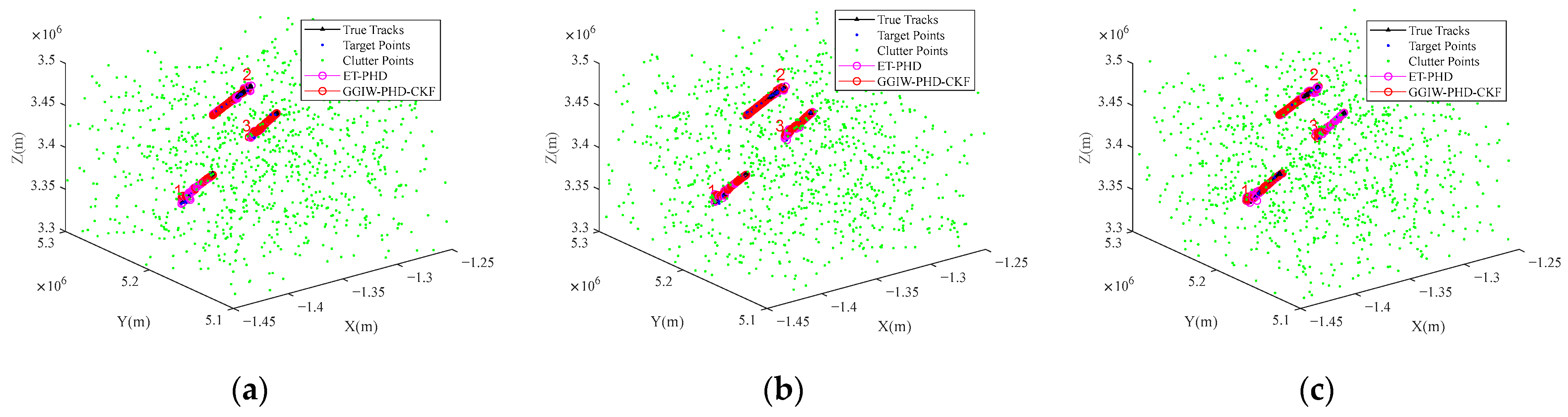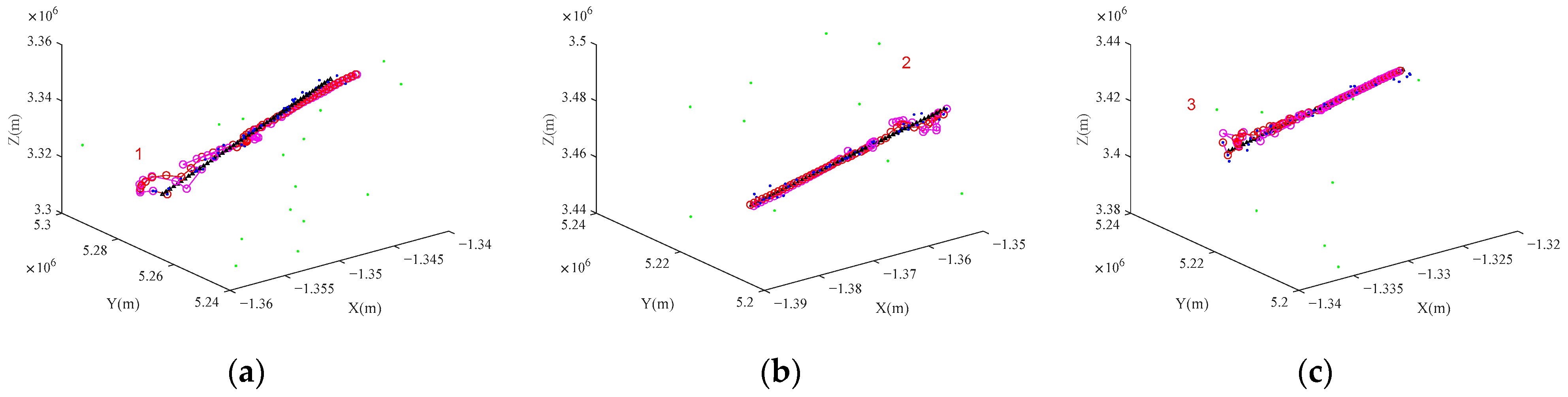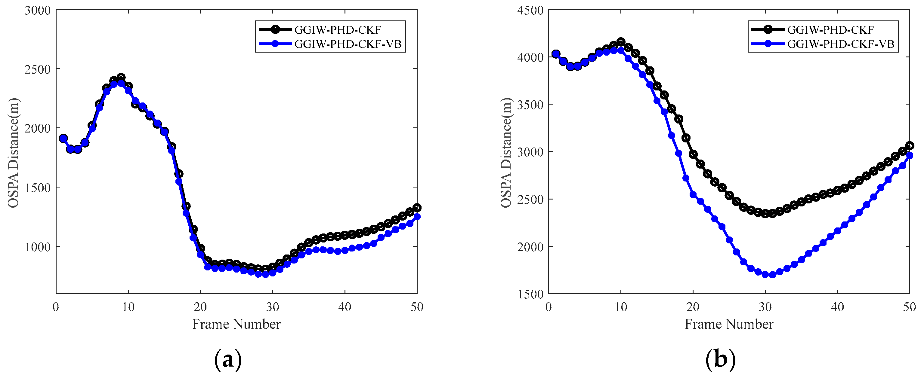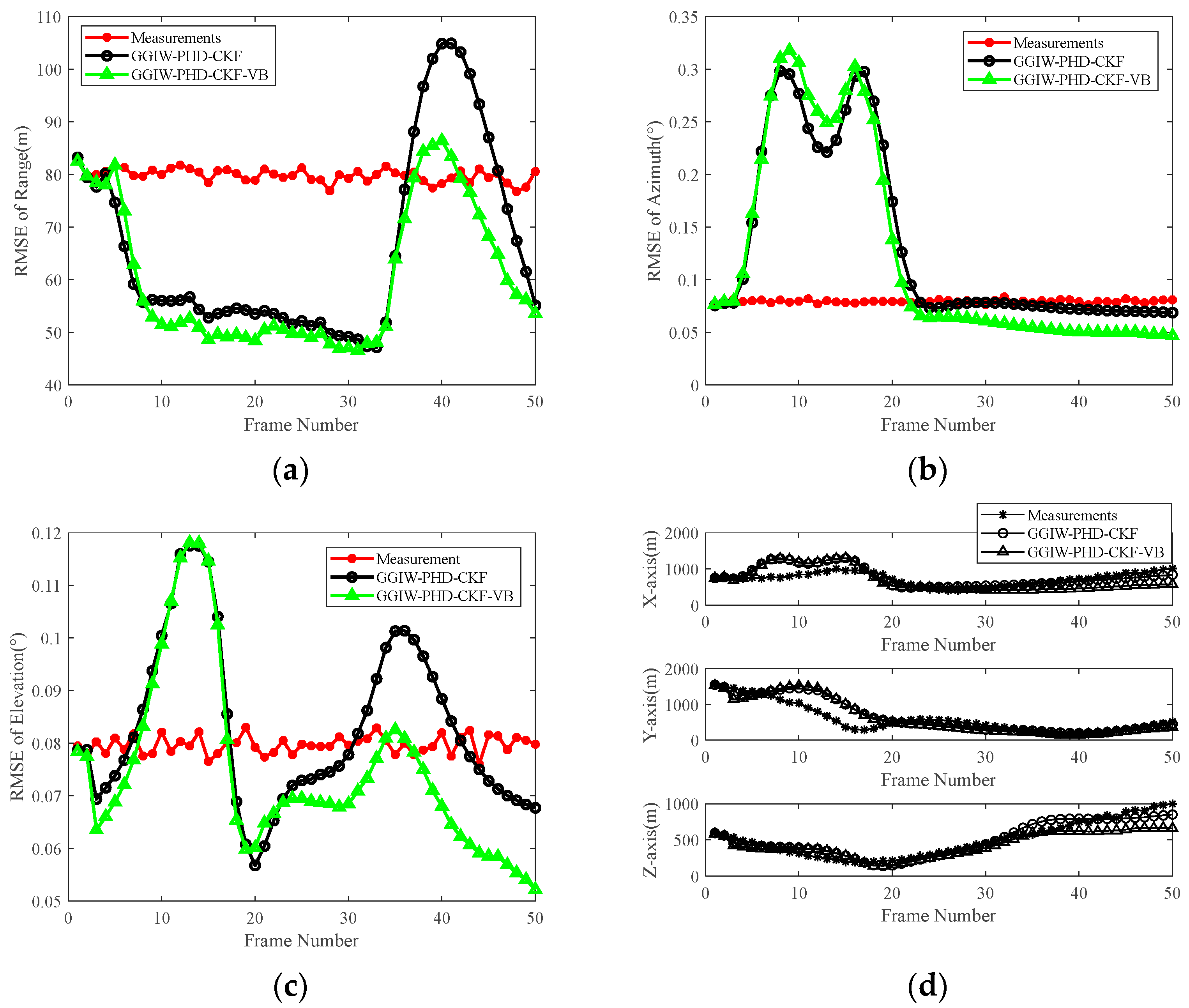Through simulations of three-dimensional aerial extended target tracking in Section 5.2, we demonstrated that the GGIW-PHD-CKF exhibits superior adaptability to targets with varying shape parameters when compared to the conventional ET-PHD filter. Comparisons of the OSPA distance and RMSE showed that GGIW-PHD-CKF has a faster convergence speed and better tracking accuracy.

Furthermore, for the problem of unknown and time-varying measurement noise, the VB method was introduced into the PHD recursion for Gaussian white noise with a zero-mean [12]. In this way, the target states, target number, and measurement noise variances could be jointly estimated. In [14], Wang et al. proposed a VB-CPHD filtering algorithm for measurement noise following Student’s t-distribution. However, the above methods were designed for point targets and are not suitable for extended targets. Therefore, we derived the closed solution to the GGIW-PHD-CKF-VB filter recursion process with Gaussian and non-Gaussian measurement noise models. 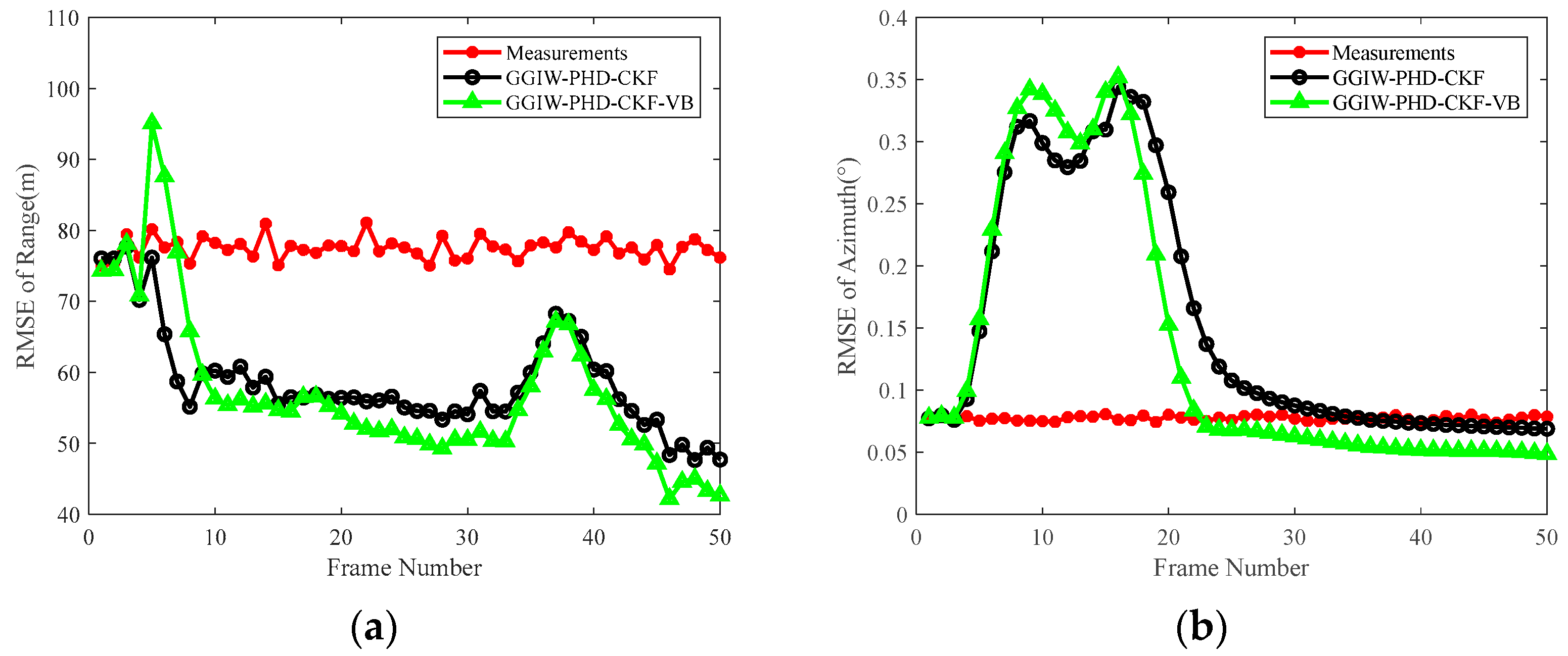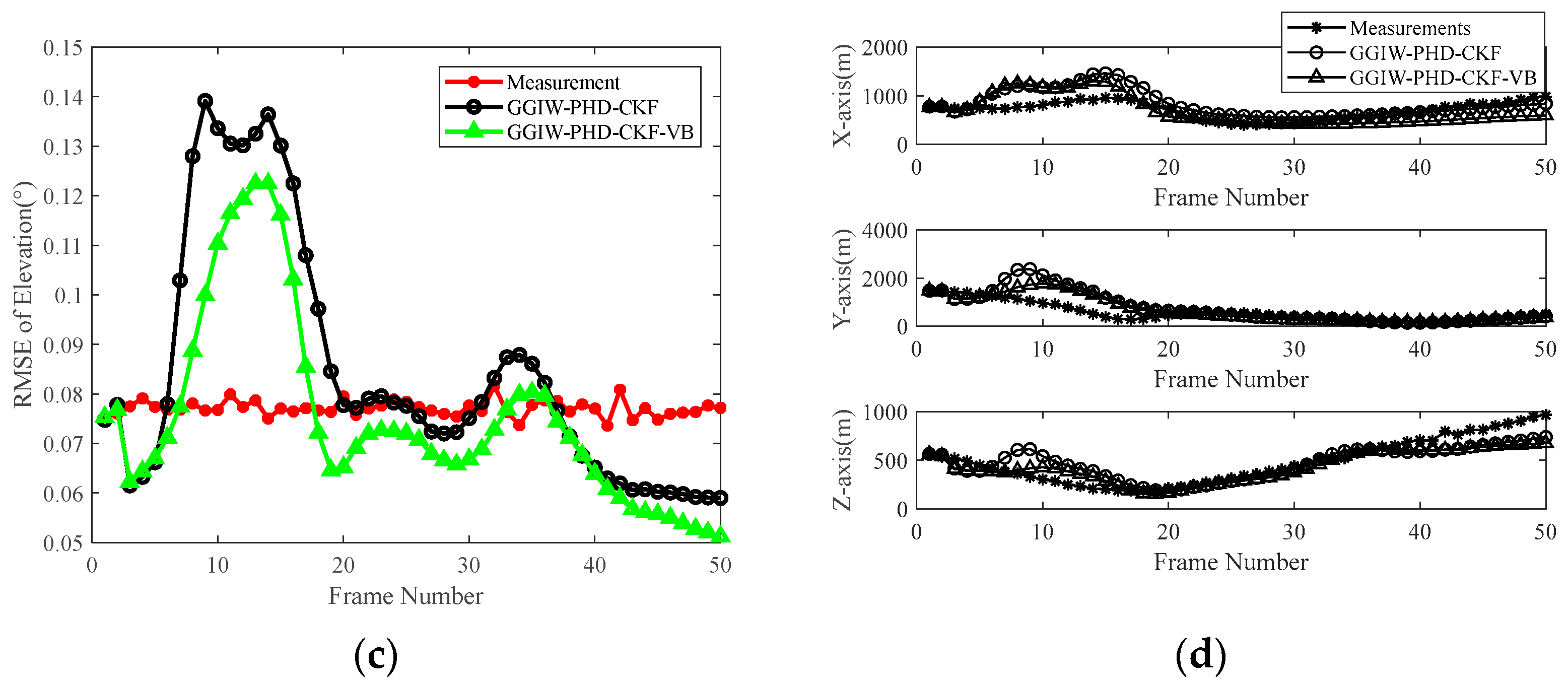The simulation experiments in Section 5.3 analyzed tracking accuracy under two distinct scenarios. The tracking results under various noise parameters demonstrated that compared with the GGIW-PHD-CKF, the GGIW-PHD-CKF-VB filter achieved lower OSPA distance and RMSE values, showing stronger robustness under different scenario parameters.

We also conducted a comparative analysis of time consumption. Simulation experiments were performed in MATLAB R2019a on a computer equipped with a 2.30-GHz Intel® Core™ processor and 16 GB of RAM. Averaged over multiple Monte Carlo runs, the ET-PHD method required 5.8 ms. In Gaussian measurement noise scenarios, the GGIW-PHD-CKF and GGIW-PHD-CKF-VB filters consumed 4.9 ms and 5.1 ms, respectively. In non-Gaussian measurement noise scenarios, the GGIW-PHD-CKF and GGIW-PHD-CKF-VB filters consumed 5.0 ms and 5.3 ms, respectively. Consequently, the GGIW-PHD-CKF-VB filter demonstrated superior computational efficiency compared to the ET-PHD method. In addition, the sampling intervals for aircraft target tracking are typically 5 s to 10 s [21]. The computational complexity of the proposed method has a considerable margin for engineering applications. However, the time consumption of practical radar target tracking is also related to factors such as the number of targets in the surveillance area and the processing capability of the hardware system, necessitating comprehensive evaluations across multiple dimensions.

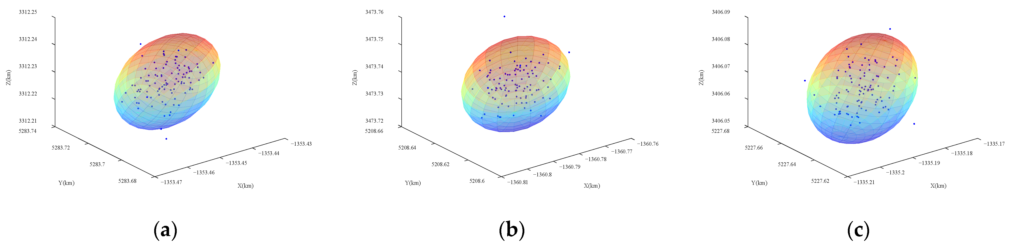
Building upon this research, future studies could be conducted to explore the following two aspects: (i) The current ellipsoidal modeling of extended targets presents certain limitations. More sophisticated and flexible shape representation methods should be investigated to better characterize target measurement distributions across varying observation angles. (ii) While this work focused on monostatic radar configurations, distributed multistatic designs could significantly enhance the tracking accuracy by enabling multi-perspective observation and mutual coverage compensation. Subsequent research should extend the proposed methodology to multistatic radar tracking scenarios.

7. Conclusions

In this study, we proposed a robust tracking method for aerial extended targets using space-based wideband radar. The main contributions of this paper are summarized as follows: (i) Building upon the space-based radar observation geometry, we established a comprehensive three-dimensional state model for aerial extended targets. (ii) We integrated a three-dimensional spherical–radial cubature rule into the GGIW-PHD filtering framework, explicitly addressing the nonlinear observation challenges. (iii) We derived the recursive procedures for the GGIW-PHD-CKF-VB filter for both Gaussian and Student’s t-distributed measurement noise models, enhancing the robustness of target tracking under uncertain measurement noise conditions. Through simulation scenarios designed with different extended target shape parameters, we validated the tracking effectiveness of the GGIW-PHD-CKF in space-based observation scenarios. Additional simulations with varying measurement noise parameters demonstrated the tracking robustness of the GGIW-PHD-CKF-VB filter. A comparative analysis of the OSPA distance and RMSE across different observation coordinates confirmed that the proposed method achieves superior tracking performance compared to traditional methods.

References

1. Chen, J.; Huang, P.; Xia, X.; Chen, J.; Sun, Y.; Liu, X. Multichannel signal modeling and AMTI performance analysis for distributed space-based radar systems. IEEE Trans. Geosci. Remote Sens. 2022, 60, 1–24. [Google Scholar] [CrossRef]
2. Zhang, J.; Ding, T.; Zhang, L. Longtime coherent integration algorithm for high-speed maneuvering target detection using space-based bistatic radar. IEEE Trans. Geosci. Remote Sens. 2022, 60, 1–16. [Google Scholar] [CrossRef]
3. Liu, Z. Interference Suppression for Space-Borne SAR and Precise Imaging of Space Object. Ph.D. Thesis, XiDian University, Xi’an, China, 2014. [Google Scholar] [CrossRef]
4. Vo, B.N.; Ma, W.K. The Gaussian mixture probability hypothesis density filter. IEEE Trans. Signal Process. 2006, 54, 4091–4104. [Google Scholar] [CrossRef]
5. Jeong, T.T. Particle PHD filter multiple target tracking in sonar image. IEEE Trans. Aerosp. Electron. Syst. 2007, 43, 409–416. [Google Scholar] [CrossRef]
6. Mahler, R. PHD filters for nonstandard targets, I: Extended targets. In Proceedings of the International Conference on Information Fusion, Seattle, WA, USA, 6–9 July 2009; pp. 915–921. [Google Scholar]
7. Koch, J.W. Bayesian approach to extended object and cluster tracking using random matrices. IEEE Trans. Aerosp. Electron. Syst. 2008, 44, 1042–1059. [Google Scholar] [CrossRef]
8. Granström, K.; Orguner, U. A phd filter for tracking multiple extended targets using random matrices. IEEE Trans. Signal Process. 2012, 60, 5657–5671. [Google Scholar] [CrossRef]
9. Granström, K.; Lundquist, C.; Orguner, O. Extended target tracking using a gaussian-mixture PHD filter. IEEE Trans. Aerosp. Electron. Syst. 2012, 48, 3268–3286. [Google Scholar] [CrossRef]
10. Granström, K.; Natale, A.; Braca, P.; Ludeno, G.; Serafino, F. Gamma gaussian inverse wishart probability hypothesis density for extended target tracking using X-Band marine radar data. IEEE Trans. Geosci. Remote Sens. 2015, 53, 6617–6631. [Google Scholar] [CrossRef]
11. Sarkka, S.; Nummenmaa, A. Recursive noise adaptive kalman filtering by variational bayesian approximations. IEEE Trans. Autom. Control. 2009, 54, 596–600. [Google Scholar] [CrossRef]
12. Zhang, G.; Lian, F.; Han, C.; Han, S. An improved PHD filter based on variational Bayesian method for multi-target tracking. In Proceedings of the International Conference on Information Fusion, Salamanca, Spain, 7–10 July 2014; pp. 1–6. [Google Scholar]
13. Li, W.; Jia, Y.; Du, J.; Zhang, J. PHD filter for multi-target tracking with glint noise. Signal Process. 2014, 94, 48–56. [Google Scholar] [CrossRef]
14. Wang, J. Research on Algorithms of Multi Targets Tracking Under Unknown Measurement Noise. Master’s Thesis, XiDian University, Xi’an, China, 2015. [Google Scholar] [CrossRef]
15. Yang, D. Multi-Sensor Target Tracking Algorithm Based on Probability Hypothesisi Density Filter Under Unkown Scene Parameters. Ph.D. Thesis, XiDian University, Xi’an, China, 2019. [Google Scholar] [CrossRef]
16. Arasaratnam, I.; Haykin, S. Cubature kalman filters. IEEE Trans. Autom. Control. 2009, 54, 1254–1269. [Google Scholar] [CrossRef]
17. Kellner, D.; Klappstein, J.; Dietmayer, K. Grid-based DBSCAN for clustering extended objects in radar data. In Proceedings of the IEEE Intelligent Vehicles Symposium, Madrid, Spain, 3–7 June 2012; pp. 365–370. [Google Scholar] [CrossRef]
18. Li, W.; Jia, Y.; Du, J.; Zhang, J. PHD filter for multi-target tracking by variational Bayesian approximation. In Proceedings of the IEEE Conference on Decision & Control, Firenze, Italy, 10–13 December 2013; pp. 7815–7820. [Google Scholar] [CrossRef]
19. He, Y.; Xiu, J.; Guan, X. Radar Data Processing with Applications; Publishing House of Electronics Industry: Beijing, China, 2013. [Google Scholar]
20. Schuhmacher, D.; Vo, B.T.; Vo, B.N. A consistent metric for performance evaluation of multi-object filters. IEEE Trans. Aerosp. Electron. Syst. 2008, 56, 3447–3457. [Google Scholar] [CrossRef]
21. Li, X.R.; Bar-Shalom, Y. Design of an interacting multiple model algorithm for air traffic control tracking. IEEE Trans. Control Syst. Technol. 1993, 1, 186–194. [Google Scholar] [CrossRef]
Figure 1. Observation geometry model of space-based radar.
Remotesensing 17 02360 g001
Figure 2. Simulation scenario: (a) the view of STK; (b) the spatial positional relationship in the ECEF coordinate system.
Remotesensing 17 02360 g002
Figure 3. OSPA distance comparisons: (a) scenario 1; (b) scenario 2; (c) scenario 3.
Remotesensing 17 02360 g003
Figure 4. Tracking result comparisons: (a) scenario 1; (b) scenario 2; (c) scenario 3.
Remotesensing 17 02360 g004
Figure 5. Tracking result comparisons of scenario 1: (a) target 1; (b) target 2; (c) target 3.
Remotesensing 17 02360 g005
Figure 6. Tracking result comparisons of scenario 2: (a) target 1; (b) target 2; (c) target 3.
Remotesensing 17 02360 g006
Figure 7. Tracking result comparisons of scenario 3: (a) target 1; (b) target 2; (c) target 3.
Remotesensing 17 02360 g007
Figure 8. Target shape estimation results of scenario 1: (a) target 1; (b) target 2; (c) target 3.
Remotesensing 17 02360 g008
Figure 9. Target shape estimation results of scenario 2: (a) target 1; (b) target 2; (c) target 3.
Remotesensing 17 02360 g009
Figure 10. Target shape estimation results of scenario 3: (a) target 1; (b) target 2; (c) target 3.
Remotesensing 17 02360 g010
Figure 11. OSPA distance comparison: (a) scenario 1; (b) scenario 2.
Remotesensing 17 02360 g011
Figure 12. RMSE comparison of scenario 1: (a) range; (b) azimuth; (c) elevation; (d) XYZ in the ECEF coordinate system.
Remotesensing 17 02360 g012
Figure 13. RMSE comparison of scenario 2: (a) range; (b) azimuth; (c) elevation; (d) XYZ in the ECEF coordinate system.
Remotesensing 17 02360 g013
Figure 14. OSPA distance comparison: (a) v = 10; (b) v = 20.
Remotesensing 17 02360 g014
Figure 15. RMSE comparison ( v = 10): (a) range; (b) azimuth; (c) elevation; (d) XYZ in the ECEF coordinate system.
Remotesensing 17 02360 g015aRemotesensing 17 02360 g015b
Figure 16. RMSE comparison ( v = 20): (a) range; (b) azimuth; (c) elevation; (d) XYZ in the ECEF coordinate system.
Remotesensing 17 02360 g016