Restricted Label-Based Self-Supervised Learning Using SAR and Multispectral Imagery for Local Climate Zone Classification

Abstract

Deep learning techniques have garnered significant attention in remote sensing scene classification. However, obtaining a large volume of labeled data for supervised learning (SL) remains challenging. Additionally, SL methods frequently struggle with limited generalization ability. To address these limitations, self-supervised multi-mode representation learning (SSMMRL) is introduced for local climate zone classification (LCZC). Unlike conventional supervised learning methods, SSMMRL utilizes a novel encoder architecture that exclusively processes augmented positive samples (PSs), eliminating the need for negative samples. An attention-guided fusion mechanism is integrated, using positive samples as a form of regularization. The novel encoder captures informative representations from the unannotated So2Sat-LCZ42 dataset, which are then leveraged to enhance performance in a challenging few-shot classification task with limited labeled samples. Co-registered Synthetic Aperture Radar (SAR) and Multispectral (MS) images are used for evaluation and training. This approach enables the model to exploit extensive unlabeled data, enhancing performance on downstream tasks. Experimental evaluations on the So2Sat-LCZ42 benchmark dataset show the efficacy of the SSMMRL method. Our method for LCZC outperforms state-of-the-art (SOTA) approaches.

1. Introduction

A classification method called Local Climate Zone (LCZ) classification is used to group urban and non-urban areas according to their climatic and environmental features. When describing the microclimates of certain regions, LCZs take into account elements such as vegetation, surface types, and urban morphology. By using supervised learning [1], we can automatically classify different urban and rural zones into meaningful climate categories, but challenges like the need for large, high-quality annotated datasets and problems with data annotation can impede progress. By addressing these issues, self-supervised learning significantly increases the scalability and efficacy of LCZ classification, particularly in cases of limited resources. Local climate zones are divided into two primary categories: urban LCZs and natural LCZs. Urban LCZs pertain to urban areas and are numbered from LCZ1 to LCZ10, while natural LCZs are associated with non-urban areas, represented by LCZA to LCZG. Figure 1 describes each climate zone, and further details are provided in [2].

Self-supervised learning is used to learn representations from unlabeled data. However, a key challenge in SSL lies in learning effective representations without relying on negative samples, which has been a cornerstone of many traditional SSL approaches. Existing methods, such as contrastive learning techniques including MoCo [3], often depend on the construction of negative samples to enforce distinct feature representations. However, negative samples similarity issue may limit the performance, in [4] authors overcame this issue with clustering approach but still the performance is limited by negative samples. Data-to-Vector [5] has demonstrated potential in managing different modalities, but it encounters difficulties if the data is lacking diversity.

We aim to contribute to the development of SSL techniques that can effectively learn meaningful representations from positive pairs alone. This is crucial for advancing the applicability of SSL, as negative samples may not always be available or well defined.

Supervised learning methods are also used for LCZC, but their reliance on labeled data, which are often costly and time-consuming to obtain, remains a major drawback. Additionally, these techniques are prone to overfitting, particularly when the amount of labeled data is limited.

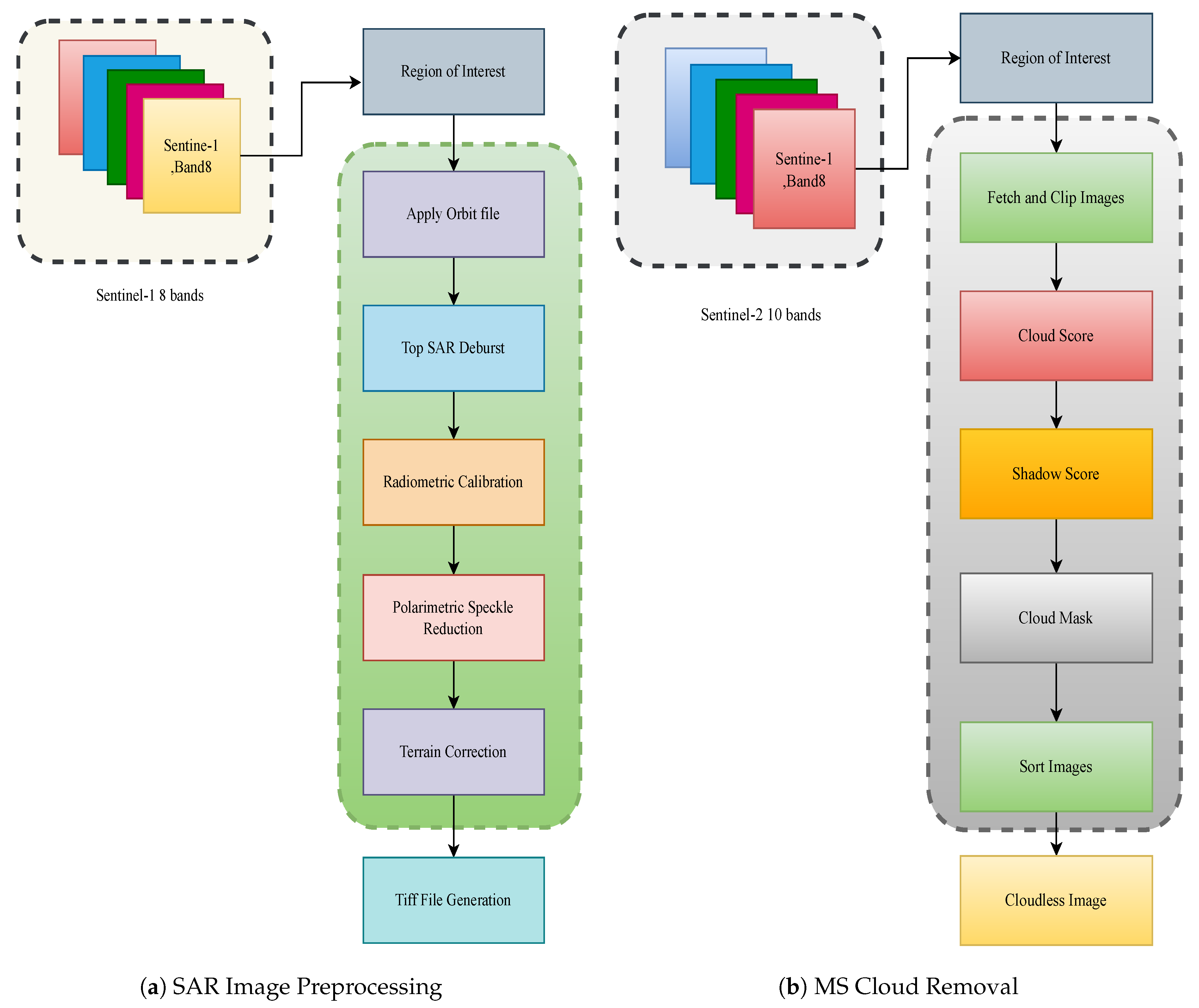
SAR and MS data have been used for LCZ classification because of their large imaging widths [6]. MS image interpretation is relatively easy because reflectance and emission from ground objects can provide sufficient details [7]. However, clouds and atmospheric conditions can make temporal requirements difficult for MS images [8]. In contrast to MS imaging, terrain and object backscattering affect SAR images—in particular, the form, shape, and composition of objects. Additionally, SAR has the unique feature of coherent imaging, which means it captures amplitude and phase information [9]. Moreover, SAR can penetrate through clouds and provides all-day image acquisition capability. However, SAR images are less intuitive to interpret and more challenging compared to MS images due to a limited number of bands and issues such as speckle noise, non-vertical range imaging, projected shortening, signal voids, surface overlap distortion, and shadowing effects [10]. Given the complementary nature of MS and SAR data, the fusion of MS and SAR has been used for LCZC [11]. In this paper, we introduce an SSL method built upon an innovative fusion network, drawing inspiration from BYOL [12].

Recent studies on Local Climate Zone Classification (LCZC) have explored various methodologies, datasets, and applications. In [13], a classification approach for LCZs in Xi’an City was proposed, leveraging 192 spatial indicators and remote sensing (RS) data. Expanding on large-scale LCZ mapping, ref. [14] developed comprehensive LCZ land use datasets for key Chinese cities and urban clusters to enhance urban climate and environmental modeling. The role of LCZC in urban heat island (UHI) analysis was examined in [15], where Zhuhai-1 satellite imagery was used to study daytime temperature variations. Similarly, ref. [16] investigated LCZ transformations over time in five major global cities, providing insights into urban climate dynamics. A broader review of LCZC methodologies and applications was conducted in [17], contributing valuable perspectives for urban climate research.

The practical applications of LCZC in sustainable urban development were highlighted in [18], while [19] applied LCZC to identify surface urban heat islands (SUHIs) and improve the understanding of urban thermal effects. The relevance of LCZC for ventilation assessment in urban planning was explored in [20]. Spatio-temporal variations of SUHIs in Beijing and their correlation with population density were analyzed in [21]. Additionally, ref. [22] reviewed LCZ mapping applications across European cities, identifying emerging trends in urban environmental studies. Studies such as that reported in [23] have assessed the effectiveness of LCZC for land surface temperature (LST) analysis, focusing on UHI pattern variability.

Advancements in data fusion techniques for LCZC have also been explored. In [24], the integration of multispectral (MS) and PALSAR-2 data was investigated for LCZ classification in Nanchang, China. Deep learning methods such as a multi-cascaded fusion network [25] and a dual graph convolutional neural network (CNN) [26] have been introduced to improve LCZ classification accuracy. The dynamic changes in LCZs across three cities and their impact on the UHI phenomenon were examined in [27]. Furthermore, ref. [28] evaluated the thermal characteristics of Riyadh’s LCZs and their implications for urban planning. Seasonal UHI analyses were conducted in Wuhan using LCZ classification in [29], while [30] explored spatial trends in urban environments through LCZ classification. Variations in LCZs across three Yangtze River mega cities were studied in [31]. The application of SAR for global LCZ classification was discussed in [32], while [33] investigated the fusion of SAR and multispectral data for LCZC using a dual-branch CNN.

SSL methods based on generative networks like the Autoencoder (AE) architecture [34] are based on the encoding and reconstruction of input data. The model is simple but suffers from overfitting and cannot capture complex distributions, which limits the generalization ability of model. Sparse AEs [35] are based on sparsity constraints to improve efficiency. However, the sparsity constraint can reduce the model’s expressiveness and may lead to instability during training if not carefully tuned. Denoising AEs [36] focuses on reconstructing clear images from noisy inputs, which helps in learning robust representations. However, they struggles when noise levels are high or when the noise distribution is not well understood, requiring a large amount of clean data for optimal performance. Variational Autoencoders (VAEs) [37] model the data distribution by encoding the input into a normal distribution. While VAEs have gained popularity for their probabilistic approach, the assumption of a Gaussian distribution can be restrictive, leading to poor results in more complex datasets. Masked Autoencoders (MAEs) [38] use random masking of image patches and leverage vision transformers for reconstruction. While MAEs have demonstrated strong performance on various vision tasks, they require significant computational resources and may lose fine-grained details during reconstruction due to masking.Generative Adversarial Networks (GANs) [39] are among the most influential models in generative learning. They consist of two neural networks—a generator and a discriminator—that are trained adversarially to produce realistic data. Adversarial Autoencoders (AAEs) [40] combine the principles of VAEs and GANs by incorporating adversarial training into the autoencoder framework. BiGANs (Bidirectional GAN) [41] extend GANs by adding an encoder that maps data samples to their latent representations. This additional encoder increases the model’s complexity and computational cost while also introducing new challenges in balancing the training of both the generator and encoder.

One of the foundational techniques in SSL is negative sampling, which aims to maximize the distance between dissimilar data points. Methods such as triplet Loss [42], MoCo, and SimCLR [43] have proven effective in various single-mode applications. These approaches suffers from negative sample selection and require large batch sizes. DeepCluster [44] and SwAV [45] generate pseudo-labels for contrastive learning but suffer from poor computational efficiency. DINO [46] is based on positive sample generation but suffers from hyperparameter tuning and scaling issues. Barlow Twins [47] and VICReg [48] are based on redundancy reduction but suffer from loss of features and instability during training.

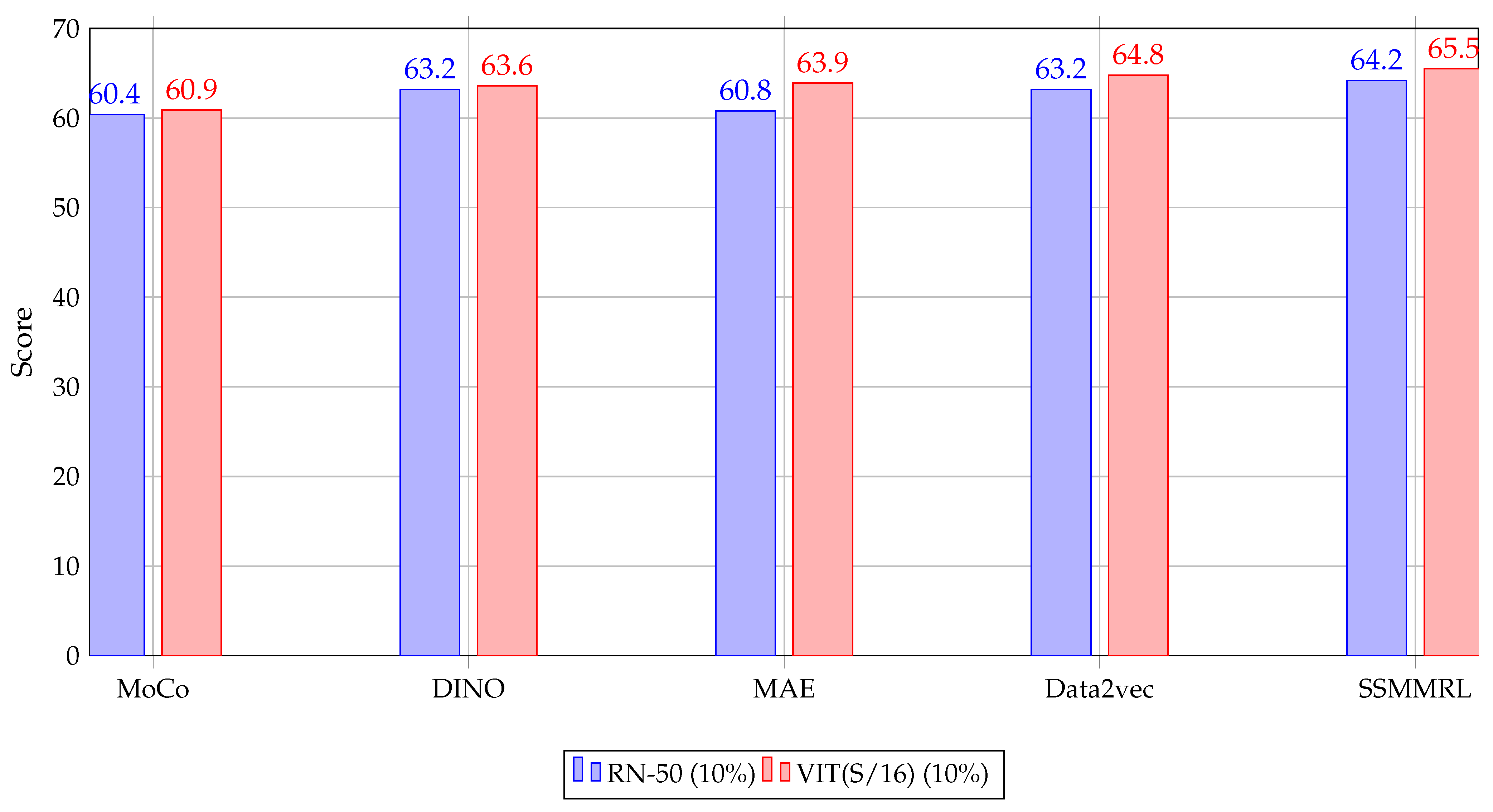
Existing SSL methods based on negative sampling, clustering, knowledge distillation, and redundancy reduction have improved the performance but still suffer when applied to multimodal data. However SSMMRL is more efficient and scalable, making it a promising solution for multi-modal classification.

The advantages of using only positive samples for model training include the simplicity of the objective function as compared to using negative and positive samples. Contrastive loss due to the use of positive and negative samples may cause instability if the samples are unbalanced and large. Models based on positive samples are more efficient and perform better in cases of limited labels.

Main Contribution

The main contributions of this work are listed below. It is pertinent to mention that, unlike BYOL, our SSMMRL has three branches, namely online, target, and fusion branches, whereas BYOL has two branches, namely teacher and student branches. SSMMRL offers greater flexibility and adaptability, making it suitable for more complex and diverse tasks that involve multiple views or modalities.

• We propose a method that actively combines positive samples to create a new fused sample, driven by an attention mechanism. By encouraging the model to create more useful features and projections from aggregated data, this regularization technique improves feature generalization.
• An additional fusion branch is added to extract meaningful features from the SAR and multispectral data and reduce overall loss.
• A dynamic convolutional module is proposed that works with different input sizes by dynamically modifying the mixed input channels to support the attention strategy.
• The suggested SSL approach requires less labeled data and performs better on multi-modal data when compared to other self-supervised learning approaches.

The structure of this article is outlined as follows. Section 2 describes study areas. Section 3 presents the methodology. Section 4 introduces the datasets and experimental settings. Section 5 is about obtained results and Section 6 is about discussion. Section 7 provides the conclusion of the article and future research.

2. Study Area

In this article, six cities were selected for performance evaluation, namely Lagos, Wuhan, Rome, Munich, Sydney, and Turin. The Google imagery of regions of interest (ROIs) for all these cities is shown in Figure 2. The global map of these cities is shown in the Figure 3. The exact coordinates of the ROIs are given in

Table 1. Regions of interest (ROIs) for selected cities.

City	Bottom-Left Coordinates (Lat, Lon)	Top-Right Coordinates (Lat, Lon)
Munich	47.89375°N, 11.33125°E	48.36875°N, 11.80625°E
Lagos	6.41875°N, 3.35625°E	6.49375°N, 3.43125°E
Rome	41.6375°N, 12.21875°E	42.1375°N, 12.74375°E
Turin	44.85625°N, 7.46875°E	45.28125°N, 7.89375°E
Sydney	−34.20625°S, 150.9°E	−33.53125°S, 151.45°E
Wuhan	30.26875°N, 113.95625°E	30.89375°N, 114.58125°E

.

3. Methodology

In this section, the frame work for SSMMRL is discussed. The methodology involves data preprocessing and augmentation, feature extraction using a dynamic convolution, squeeze and excitation, and self-supervised training with a fusion-branch framework. The fusion branch leverages an attention-based mechanism to fuse information from two augmented views of the input, enhancing the learned representations.

3.1. Proposed Framework

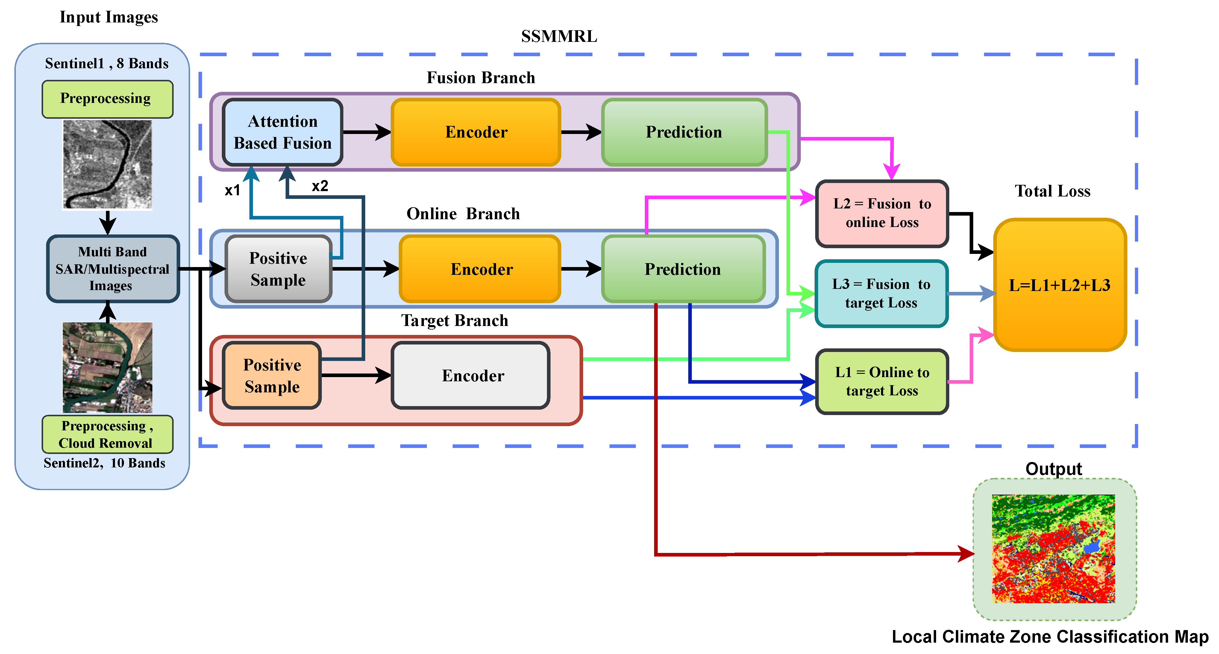
The proposed framework is shown in Figure 4. Multi-spectral and SAR images are preprocessed and applied to the online, target, and fusion branches. The input image (x) is passed through the positive sample generator, and it produces $x_1$ for the online branch and $x_2$ for the target branch. Both $x_1$ and $x_2$ are passed through the feature encoder to generate representations ($z_1^{\mathrm{on}}$ and $z_2^{\mathrm{on}}$), respectively. The online and target encoders are represented as $f_{\theta \mathrm{on}}$, and $f_{\theta \mathrm{tg}}$ respectively.

The predictions are generated from the representations, and the predictor is denoted by g. The fusion branch gets $x_1$, $x_2$. Attention-based fusion is applied to achieve better feature representation. The predictions from the online and fusion branches, along with the encoder outputs, are used to compute the weighted loss. The target branch network is updated using online network parameters. Initially, the network is pretrained without any labeled samples; then, a few annotated training samples are used for fine-tuning and classification tasks.

The outputs of the online feature extractor are ($z_1^{\mathrm{on}}$ and $z_2^{\mathrm{on}}$), while the representation of the target feature extractor are ($z_1^{\mathrm{tg}}$, $z_2^{\mathrm{tg}}$).

The augmented views ($x_1$ and $x_2$) are generated from x.

$$\begin{array}{cc}\hfill z_1^{\mathrm{on}}& =f_{\theta \mathrm{on}}\left(x_1\right),z_2^{\mathrm{on}}=f_{\theta \mathrm{on}}\left(x_2\right)\hfill \end{array}$$

(1)

$$\begin{array}{cc}\hfill z_1^{\mathrm{tg}}& =f_{\theta \mathrm{tg}}\left(x_1\right),z_2^{\mathrm{tg}}=f_{\theta \mathrm{tg}}\left(x_2\right)\hfill \end{array}$$

(2)

Representations are mapped to predictions using the $g(·)$ operator, called the predictor.

$$\begin{array}{c}\hfill p_1=g\left(z_1^{\mathrm{on}}\right),p_2=g\left(z_2^{\mathrm{on}}\right),p_{\mathrm{fused}}=g\left(z_3^{\mathrm{fusion}}\right).\end{array}$$

(3)

An attention mechanism is applied to obtain the attention map. The attention map helps in weighting the importance of each pixel or feature in the input images, resulting in a hybrid sample.

The target branch network (${\theta }_{\mathrm{tg}}$) is updated using online network parameters.

$$\begin{array}{c}\hfill {\theta }_{\mathrm{tg}}\leftarrow {\tau }_s{\theta }_{\mathrm{tg}}+(1-{\tau }_s){\theta }_{\mathrm{on}}\end{array}$$

(4)

where ${\tau }_s$ is a momentum parameter. Initially, the network is pretrained without any labeled samples; then, a small portion of annotated samples is used for fine-tuning and classification tasks.

3.2. Preprocessing and Sample Generation

Augmentation includes a random crop with specific aspect-ratio and scale constraints, as well as a random horizontal flip. A random crop is applied, with the height (ph) in the range of [0.5, 1.0] and the width (pw) based on the height (ensuring the width is between 0.67 and 1.0 times the height). The crop size is fixed at 32 × 32. A random horizontal flip with 0.5 probability is used. The random crop and horizontal flip are applied sequentially to the input image (x). The augmented image is returned, maintaining the correct number of channels (though this part is implicit, since the number of channels is maintained through the transformations). The combined augmentation pipeline can be expressed as follows:

$$\tilde{x}=T_{\mathrm{f}}\left(T_{\mathrm{c}}\left(x\right)\right),$$

(5)

where the augmented image ($\tilde{x}$) is obtained by applying a random crop ($T_{\mathrm{c}}$), then a horizontal flip ($T_{\mathrm{f}}$).

It is pertinent to mention that data augmentation is a powerful tool for improving the performance and generalization of machine learning models, especially when training data are limited. It helps the model learn more robust features by introducing variability in the data, making it more capable of handling real-world data. However, it is important to apply augmentations judiciously, as too many extreme transformations can lead to overfitting or unrealistic data, thereby decreasing the model’s ability to generalize. It also comes with trade-offs in terms of increased training time and computational cost. Hence, a balanced approach, where augmentations are both realistic and diverse, is key to leveraging the full potential of this technique. The ablation study shows the effect of data augmentation.

3.3. Encoder Architecture

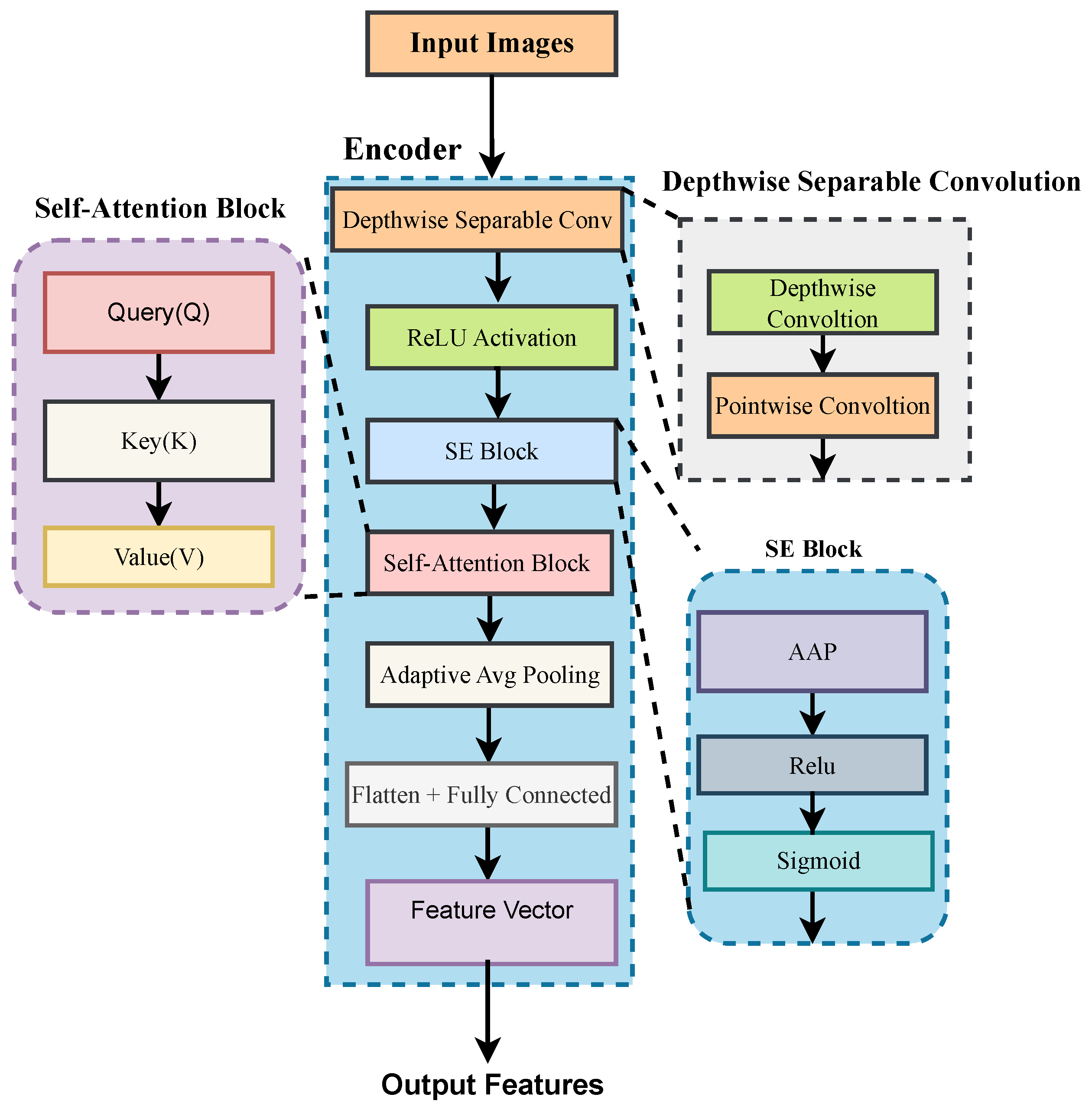
A detailed diagram of the encoder is shown in Figure 5. The Dynamic-Separable Convolution-Encoder (DS-Conv) is a neural network that integrates depthwise separable convolutions, a squeeze-and-excitation module [SE], and a self-attention block [SAB] to encode the input data. It also applies an adaptive average-pooling (AAP) operation to minimize the spatial dimensions and  a fully connected layer to output the final feature representation. Depthwise Separable Convolution [DSC] separates the depth-wise and point-wise convolutions to minimize the computation. Unlike normal convolutions, each channel is applied independently with a unique filter. This results in fewer parameters. After applying depth-wise convolution, point-wise convolution is performed. The output of DSC is applied to the SEB. The SEB recalibrates feature maps by learning channel-wise dependencies, which consist of A-AP, Relu, and sigmoid modules. The objective of SE is to capture global information (squeezing) and selectively emphasize certain features (excitation), it focuses on more important features and ignore less important features. After SE, the features are passed through the self-attention block (SAB), which contains query (Q), key (K), and value (V) modules. The attention weights are applied to the value matrix, and the result is summed with the original input tensor. The objective is to compute the attention score and identify important data. The output of the SAB is passed through adaptive average pooling (A-AP) and, lastly, flattened.

Algorithm 1 shows the entire pretraining process. The unlabeled data (x) are used to obtain the pretrained encoder (f). The algorithm shows all steps, including positive sample generation, loss computation, and backpropagation.

Algorithm 1 Self-Supervised Learning Pretraining

Input: Unlabeled training images x Output: Trained encoder f   1: Define:   2:     $psg(·)$: function of positive sample generation   3:     $abm(·)$: function of attention-based mixing   4: for each x in dataset do   5:    Compute $x_1$ and $x_2$ using $psg\left(x\right)$   6:    Compute $x_3$ using $abm(x_1,x_2)$   7:    Extract features $z_1,z_2$ from $f\left(x_1\right),f\left(x_2\right)$   8:    Compute $z_f$ using $f\left(x_3\right)$   9:    Extract prediction features $p_1,p_2,p_{fused}$ from $g\left(x_1\right)$, $g\left(x_2\right)$, and $g\left(f\left(x_3\right)\right)$ 10:    Compute ${\mathcal{L}}_{\mathrm{online-target}}$ using Equation (7) 11:    Compute ${\mathcal{L}}_{\mathrm{fusion-online}}$ using Equation (8) 12:    Compute ${\mathcal{L}}_{\mathrm{fusion-target}}$ using Equation (9) 13:    Compute the final loss ${\mathcal{L}}_{\mathrm{final}}$ using Equation (10) 14:    Backpropagate to update the encoder f and predictor g 15: end for

Similarly, Algorithm 2 shows the entire process of fine tuning of the pretrained model. In this step, labeled data are used, and loss is computed using cross entropy between labeled samples and predicted samples.

Algorithm 2 Fine Tuning a Pretrained Encoder for Classification

Input: Training dataset file, Pretrained encoder weights, Number of epochs Output: Fine-tuned classifier   1: Load Training Data:   2:     Load $x_{\mathrm{train}},y_{\mathrm{train}}$ from $train\_file$   3:     Convert labels to class indices using $argmax$   4:     Create train dataset and DataLoader   5: Load Pretrained Encoder:   6:     Define encoder f with depthwise separable convolution, SE block, and self-attention   7:     Load pretrained weights from $pretrained\_path$   8: Define Classifier:   9:     Construct classifier with encoder f followed by a fully connected layer 10:     Move classifier to device (GPU or CPU) 11:     Define optimizer (Adam) and loss function (CrossEntropyLoss) 12: Fine-Tuning Process: 13: for $epoch$ $=1$ to E do 14:    Set classifier to training mode 15:    Initialize total loss to zero 16:    for each batch $(x,y)$ in train loader do 17:      Copy $x,y$ to device 18:      Compute predictions $\widehat{y}=\mathrm{classifier}\left(x\right)$ 19:      Calculate loss $\mathcal{L}=\mathrm{Cross-Entropy-Loss}(\widehat{y},y)$ 20:      Perform backpropagation and update model parameters 21:      Accumulate loss 22:    end for 23:    Print average loss for the epoch 24: end for 25: Return: Fine-tuned classifier

Algorithm 3 is used to find the classification results by using fine-tuned encoder and test data without labels. Once the predicted labels are stored, they can be used later to find the confusion matrix, output accuracy, average accuracy, and kappa values.

Algorithm 3 Evaluation of Fine-Tuned Classifier on Test Data

Input: Testing dataset file $test\_file$, Fine-tuned classifier Output: Model accuracy on test dataset   1: Load Testing Data:   2:     Load $x_{\mathrm{test}},y_{\mathrm{test}}$ from $test\_file$   3:     Convert labels to class indices using $argmax$   4:     Create test dataset and DataLoader   5: Evaluation Process:   6: Set classifier to evaluation mode   7: Initialize correct predictions counter   8: Initialize total samples counter   9: Initialize lists for true labels $y_{\mathrm{true}}$ and predicted labels $y_{\mathrm{pred}}$ 10: for batch $(x,y)$ in test loader do 11:    Copy $x,y$ to device 12:    predictions $\widehat{y}=\mathrm{classifier}\left(x\right)$ 13:    Calculate predicted labels using $argmax$ 14:    Update correct predictions and total samples 15:    Store true and predicted labels 16: end for 17: Compute accuracy as ${\displaystyle \frac{\mathrm{Correct}\mathrm{prediction}}{\mathrm{Total}}}$ 18: Print final accuracy using accuracy_score$(y_{\mathrm{true}},y_{\mathrm{pred}})$ 19: Return: Test accuracy

3.4. Attention-Based Mixing

Attention-based mixing assists the model in paying attention to different parts of data, making the network more flexible and capable of handling varying feature relationships between the two inputs. This step mixes the two input feature maps (${\mathrm{x}}_1$ and ${\mathrm{x}}_2$) based on the attention map. The attention map acts as a weighting function to blend the two inputs.

$${\mathbf{x}}_3=\mathbf{At}\odot {\mathbf{x}}_1+(1-\mathbf{At})\odot {\mathbf{x}}_2$$

(6)

where ${\mathbf{x}}_1$ and ${\mathbf{x}}_2$ are input images from the online and target branches, respectively, ${\mathbf{x}}_3$ is the final augmented image, and $\mathbf{At}$ stands for attention map.

3.5. Loss Computation

The final loss is computed as the sum of the individual losses. As there are three branches in our model, all of the branches are used to compute the final loss. The loss due to the online and target branches is called $L_{\mathrm{online-target}}$. Similarly, loss due to the fusion and online branches is called $L_{\mathrm{fusion-online}}$, and loss due to the fusion and target branches is called $L_{\mathrm{fusion-target}}$.

3.5.1. Online-to-Target Loss

In order to ensure that the representations learned by the online branch match a set of target representations, we minimize the cosine similarity loss as follows:

$${\mathcal{L}}_{\mathrm{online-target}}=-{\displaystyle \frac{1}{M}}\sum _{i=1}^M\left(\langle p_1,z_1^{\mathrm{tg}}\rangle +\langle p_2,z_2^{\mathrm{tg}}\rangle \right)$$

(7)

where:

• $\langle p_1,z_1^{\mathrm{tg}}\rangle$ represents the (cosine) similarity between $p_1$ and $z_1^{\mathrm{tg}}$;
• $\langle p_2,z_2^{\mathrm{tg}}\rangle$ represents the (cosine) similarity between $p_2$ and $z_2^{\mathrm{tg}}$; and
• M is the batch size.

3.5.2. Fusion-to-Online Loss

The online representation should be in line with the fused representation ($z_{\mathrm{fusion}}$), which is enforced by the following loss, as it is expected to capture significant information from both branches:

Loss from the fusion to the online branch is defined as follows:

$${\mathcal{L}}_{\mathrm{fusion-online}}=-{\displaystyle \frac{1}{M}}\sum _{k=1}^M\langle z_3^{\mathrm{fusion}},p_1\rangle$$

(8)

where:

• $z_3^{\mathrm{fusion}}$ is the fusion-branch representation vector and
• $p_1$ is the online branch projection.

3.5.3. Fusion-to-Target Loss

To further verify that the fused representation retains significant target information, we add the fusion-to-target loss:

$${\mathcal{L}}_{\mathrm{fusion-target}}=-{\displaystyle \frac{1}{M}}\sum _{k=1}^M\langle z_3^{\mathrm{fusion}},z_1^{\mathrm{tg}}\rangle$$

(9)

where:

• $z_3^{\mathrm{fusion}}$ is the fusion-branch representation vector and
• $z_1^{\mathrm{tg}}$ is the target representation.

3.5.4. Final Loss Function

The sum of the individual losses is expressed as

$${\mathcal{L}}_{\mathrm{final}}=\alpha {\mathcal{L}}_{\mathrm{online-target}}+\beta {\mathcal{L}}_{\mathrm{fusion-online}}+\gamma {\mathcal{L}}_{\mathrm{fusion-target}}$$

(10)

where $\alpha =0.5$, $\beta =0.5$, and $\gamma =0.5$ are are weights of individual losses controlling the contribution of each loss term. These weights allow for flexibility in balancing the different objectives during training. The dataset, augmentation technique, and model architecture are some of the variables that affect the ideal weight values. Typically, training performance is used to experimentally select the weights.

4. Data and Experimental Framework

4.1. Dataset

The So2Sat-LCZ42 [2] dataset contains co-registered SAR and Multispectral images of local climate zones.Three versions of the dataset have been released (https://github.com/zhu-xlab/So2Sat-LCZ42, accessed on 5 January 2025). In this article, version 3 is used. It consists of 352,366 samples and 48,307 test samples. The dataset was chosen for the following reasons. First, it contains cities around the world. Second, the cities have complex morphologies. Third, the number of samples is large. Fourth, the samples are collected from various cultural cities within the continent. These reasons make it a challenging dataset. The training and testing patches have dimensions of 32 × 32 pixels. Sentinel-2 has ten bands, and Sentinel-1 has eight bands, with a ground sampling distance of 10 m. Descriptions of Sentinel-1 bands are presented in

Table 2. Sentinel-1 bands.

Band	Description
1	VH channel real value, no filtering
2	VH channel imaginary value, no filtering
3	VV channel real value, no filtering
4	VV channel imaginary value, no filtering
5	VH channel filtered (Lee), intensity
6	VV channel filtered (Lee), intensity
7	Covariance matrix of diagonal real values
8	Covariance matrix of diagonal imaginary values

, and the Sentinel-2 bands are described in

Table 3. Description of Sentinel-2 data.

Band	Wavelength (nm)	Resolution (m)	Description
2	490	10	Blue
3	560	10	Green
4	665	10	Red
5	705	20, upsampled to 10	VN-IR
6	740	20, upsampled to 10	VN-IR
7	783	20, upsampled to 10	VN-IR
8	842	10	VNIR
8a	865	20, upsampled to 10	VN-IR
11	1610	20, upsampled to 10	SW-IR
12	2190	20, upsampled to 10	SW-IR

. Sentinel-1 consists of VH, HH, and VV polarization. Some of the bands are not filtered, and some are speckle-filtered by applying a Lee filter. Similarly, Sentinel-2 bands consist of multiple bands, including visible and infrared bands. We used all of the 18 bands in the training and testing process. It is pertinent to mention that MS images are normalized before testing.

4.2. Performance Evaluation and Experimental Configuration

The performance of LCZC is evaluated using Average Accuracy (AA), Output Accuracy (OA), and the kappa measure.

$$\mathrm{Output}\mathrm{Accuract}={\displaystyle \frac{\mathrm{True}\mathrm{positive}}{\mathrm{True}\mathrm{positive}+\mathrm{False}\mathrm{positive}}}$$

(11)

$$\mathrm{Average}\mathrm{Accuracy}={\displaystyle \frac{{\sum }_{i=1}^M{\mathrm{Recall}}_i}{M}}$$

(12)

$$\mathrm{ka}={\displaystyle \frac{\mathrm{OA}-\mathrm{EA}}{1-\mathrm{EA}}}$$

(13)

where OA is the observed accuracy and EA is the expected accuracy. We selected hyperparameters based on preliminary experiments. We used a batch size of 64, as it provided a good trade-off between computational efficiency and stable convergence. Smaller batch sizes (e.g., 32) resulted in noisier gradient updates, while larger batch sizes increased memory requirements without notable improvements in performance. The initial learning rate was set to 0.001. We tested alternative values (0.01, 0.0005, and 0.0001) and observed that 0.01 caused instability, while 0.0001 led to very slow convergence. A cosine decay learning-rate schedule was also used to gradually reduce the learning rate for improved optimization.

We implemented pretraining for 100 epochs with an initial learning rate of 0.001. The batch size was set as 64. The loss weights were set as $\alpha =0.5$, $\beta =0.5$, and $\gamma =0.5$. For few-shot classification, the dimension of the fully connected layer was equal to the number of local climate zones. For fine tuning, the model was trained for 100 epochs with a learning rate of 0.001 and a batch size of 64.

Table 4. Performance based on batch size and learning rate.

Batch Size	lr	OA
32	0.001	64.60%
64	0.001	64.65%

shows the effect of batch size on accuracy.

4.3. SAR and MS Preprocessing

SAR image preprocessing is a necessary step. Once the SAR and multispectral data have been downloaded, the preprocessing steps are used to generate ten MS bands and eight SAR bands, as shown in Figure 6. The entire process is shown in Figure 7 for both SAR and MS images.

Region selection is the first step where the area of interest (AOI) is selected from the larger dataset. For both SAR and MS images, it is important to define the region where further analysis will occur. This step could involve cropping or selecting a specific geographic region. The orbit file contains information about the satellite’s position and its path in space. It is required for georeferencing so that images are aligned with geographical coordinates. The technique of “debursting” involves stitching together the separate bursts of SAR images to create a single, seamless image. By eliminating any distortions caused by the sensor, radiometric calibration guarantees that the reflectance values in the picture match the true physical characteristics of the Earth’s surface. Speckle noise due to the interference of radar waves is very common; by eliminating this noise, speckle reduction techniques improve the clarity and interpretability of the images. Terrain correction is the process of modifying an image to take into consideration distortions brought about by the Earth’s surface topography, such as valleys and mountains. This stage guarantees that the image depicts the landscape. Clouds are frequently captured in MS images, which can make the land surface invisible. Cloud removal is an essential preprocessing step to eliminate these features from the data, making the analysis more accurate. Similar to SAR images, multispectral images also need to be cropped to focus on the region of interest, eliminating irrelevant areas. Cloud score computation involves identifying areas in the image that are likely to contain clouds. Cloud detection algorithms can assign a cloud score to each pixel, helping to classify and filter out cloud-covered regions. Shadows cast by clouds or terrain can also obscure the surface in multispectral images. A shadow score is computed to identify these areas, allowing for their removal or correction. After cloud and shadow removal, the remaining images are sorted or processed in a way that enhances their usability for further analysis, typically focusing on the areas of interest with clear visibility. In essence, the process involves several preprocessing steps for both SAR and multispectral images to prepare them for further analysis, ensuring that the data are clean, accurate, and ready for the next stages of processing.The outcome of MS preprocessing and SAR preprocessing is 18 bands. These bands are concatenated. The 18-band concatenated images are further divided into 32 × 32 patches. The patches are then applied to the fine tuned network for classification. For pretraining and fine tuning, only the So2satLC42 dataset is used.

Table 5. Preprocessing steps for Sentinel-1 (SAR) images.

Step	Description
1. Image Cropping	Cropping of the image to the area of interest or study region.
2. Radiometric Calibration	Conversion of digital numbers to backscatter coefficients (sigma nought).
3. Geometric Correction	Georeferencing to align with the coordinate system (e.g., UTM).
4. Noise Filtering	Speckle filtering using techniques like Lee or Gamma filters to reduce SAR noise.
5. Terrain Correction	Correction for topography using a Digital Elevation Model (DEM).
6. Image Normalization	Normalization of backscatter values to reduce temporal inconsistencies.

and

Table 6. Preprocessing steps for Sentinel-2 (Optical) images.

Step	Description
1. Image Cropping	Cropping of the image to focus on the study region or area of interest.
2. Geometric Correction	Georeferencing to map coordinates, typically based on the WGS84 datum.
3. Atmospheric Correction	Removal of clouds, haze, and aerosols using atmospheric correction models.
4. Image Normalization	Reflectance normalization for consistency across different images and times.
5. Cloud Masking	Cloud masking based on reflectance thresholds or cloud detection algorithms.

show preprocessingsteps for Sentinel-1 and Sentinel-2, respectively.

The preprocessing steps for both SAR and multispectral images have a significant impact on the final classification results.

A histogram of the testing sample is shown in Figure 8. It shows the number of samples per class for both training and testing data. It is obvious from the histogram that number of samples per class differs and needs to be balanced before training the network.

5. Results

5.1. Results Comparison

The So2satLC42 dataset is used to determine the classification accuracy. First of all, unlabeled data are used to pretrain the network. The pretraining results are presented in

Table 7. Linear evaluation [49].

No of Samples (%)	10		100
Model	RN-50	VIT (S/16)	RN-50	VIT (S/16)
MoCo	61.3	59.6	61.8	62.2
DINO	55.5	60.9	57.0	62.5
MAE	-	59.5	-	60.0
Data2vec	-	58.2	-	59.7
SSMMRL (Ours)	-	61.4	-	62.5

The bold text represents maximum OA value.

, and Figure 9 shows a comparative graph for OA with different encoders and models. We compared the results with the state-of-the-art [49] SSL models like Moco, DINO, MAE, and Data2vec. Instead of using ResNet (RN-50) or Vision Transformer (VIT), we used novel SSMMRL. The percentage of samples used for performance comparison are 10% and 100%, respectively. It is evident that SSMMRL achieved 61.4% output accuracy for 10% and 62.5% for 100% data, which is better than the rest of the algorithms.

After the pretraining, fine tuning of the model is performed using labeled data. However, very few labels are required to train the model because the model has already learned features in the pretraining stage. The results are depicted in

Table 8. Fine tuning [49].

No. of Samples (%)	10		100
Model	RN-50	VI (S/16)	RN-50	VIT (S/16)
MoCo	60.4	61.2	60.9	61.6
DINO	63.2	61.5	63.6	62.2
MAE	-	60.8	-	63.9
Data2vec	-	63.2	-	64.8
SSMMRL (ours)	-	64.2	-	65.5

The bold text represents maximum OA value.

and Figure 10. It can be seen that our model achieves better results than the other state-of-the-art models. We achieved 64.1% and 65.5% for 10% and 100% samples, respectively. Furthermore, Figure 11 shows a comparison of linear, fine-tuning, and supervised methods. Here, we increase the percentage of labeled data from 1% to 100% and evaluate the performance accordingly for pretraining, also called linear probing (LP), fine tuning (FT), and supervised learning (SL). Fine-tuning results are better than the pretraining and supervised learning results. The results were also compared with other models [50], like pseudo labels, self-ensemble, dual student, AMRAN, and transfer learning models as shown in

Table 9. Comparison of results [50].

Model	OA (%)	AA (%)	Ka
Baseline	57.59	48.47	0.5350
Pseudo label	59.83	46.01	0.5585
Self Ensemble	58.20	47.03	0.5463
DualStudent	61.98	49.10	0.5823
AMRAN	61.11	49.10	0.5745
Transfer Learning	63.66	50.27	0.6004
SSMMRL (ours)	64.95	62.27	0.6204

The bold text represents maximum OA value.

and Figure 12. SSMMRL results are better than the rest of the models in terms of OA, AA, and Ka.

In order to show that SSMMRL is computationally efficient, the training time for 100 epochs is shown for different SSL models in

Table 10. Training times of the studied SSL methods (100 epochs) [50].

Model	MoCo	DINO	MAE	DATA2VEC	SSMMRL
ResNet50	18 h	25 h	-	-	-
ViT-S/16	24 h	25 h	7 h	14 h	-
Encoder (Our)	-	-	-	-	6 h

The bold text represents minimum time for training.

using NVIDIA A100 GPUs.

A statistical test was performed to compare performance using self-supervised learning models.

Table 11. Comparison of SSMMRL with different methods using a t-test.

Method	OA (Avg)	t-Value	p-Value	Conclusions
MoCo	61.2	3.79	0.0053	SSMMRL performs significantly better than MoCo.
DINO	61.5	4.12	0.0033	SSMMRL is significantly better than DINO.
MAE	60.8	4.82	0.0013	SSMMRL is significantly better than MAE.
Data2vec	63.2	2.87	0.0209	SSMMRL performs significantly better than Data2vec.
BYOL	62.1	2.79	0.0236	SSMMRL performs significantly better than BYOL.
SSMMRL	64.2			The baseline method for comparison.

The bold text represents maximum OA value.

shows that SSMMRL is significantly better than the rest of the models. The p-value and t-value parameters were obtained by using the average value of five experiments for each model, p-values below 0.05 indicate a statistically significant difference. Similarly, high t-values indicate significant differences.

In order to evaluate the class-wise accuracy, the confusion matrix is shown in Figure 13 for OA = 64.65% and 64.95% respectively, as determined in the ablation study. The diagonal values show the overall accuracy; it can be seen that class 17 has a maximum accuracy of 99%.

Overall, the classification is effective. The detailed classification report is shown in

Table 12. Classification Report: Precision, Recall, and F1-Score.

Class	Precision	Recall	F1 Score
0	0.54	0.21	0.31
1	0.80	0.46	0.58
2	0.58	0.56	0.57
3	0.60	0.72	0.65
4	0.59	0.43	0.50
5	0.44	0.55	0.49
6	0.28	0.36	0.31
7	0.79	0.85	0.82
8	0.60	0.40	0.48
9	0.34	0.51	0.41
10	0.97	0.80	0.88
11	0.45	0.43	0.44
12	0.36	0.08	0.13
13	0.60	0.87	0.71
14	0.65	0.37	0.47
15	0.39	0.63	0.48
16	0.97	0.99	0.98
Accuracy	0.65
Macro Avg	0.58	0.54	0.54
Weighted Avg	0.66	0.65	0.64

, showing the precision, recall, and F1 score for each class.

5.2. LCZ Maps

The local climate zone classification of six cities is shown in Figure 14. The 17 classes are shown in various colors. The LCZ map shows that most of the classes are correctly classified. The maximum accuracy is achieved for class G (water). It is evident from the LCZ maps that water bodies are easily classified (shown in blue color). The accuracy for the rest of the classes is as per the confusion matrix, which is discussed earlier.

5.3. Data Visualization

A T−SNE visualization is presented in Figure 15. These plots show how the application of SSMMRL enhances the representation of data, turning initially scattered points (unlearned) into well-separated clusters (learned), reflecting the power of the learned model in organizing and extracting meaningful patterns from the data.

6. Discussion

6.1. Ablation Study

Table 13. Ablation study with structural components, loss functions, and positive sample generation methods (L1 = ${\mathcal{L}}_{\mathrm{online-target}}$, L2 = ${\mathcal{L}}_{\mathrm{fusion-online}}$, and L3 = ${\mathcal{L}}_{\mathrm{fusion-target}}$).

Experiment	Loss Function	EB	SAB	DS-Conv	A-AP	Positive Sample Generation	OA	Kp
1	L1 + L2 + L3	Yes	No	No	No	Full Augmentation Pipeline	60.85	59.97
2	L1 + L2+ L3	Yes	Yes	No	No	Full Augmentation Pipeline	61.4	60.98
3	L1 + L2 + L3	Yes	Yes	Yes	No	Full Augmentation Pipeline	64.65	61.57
4	L1 + L2	Yes	Yes	Yes	No	Full Augmentation Pipeline	61.3	59.86
5	L1 + L2	Yes	Yes	Yes	Yes	Full Augmentation Pipeline	61.5	59.95
6	L1 + L2 + L3	Yes	Yes	Yes	Yes	Full Augmentation Pipeline	64.95	62.4
7	L1 + L2+ L3	Yes	Yes	Yes	Yes	Horizontal Flip	63.91	61.71
8	L1 + L2+ L3	Yes	Yes	Yes	Yes	Vertical Flip	63.85	61.75
9	L1 + L2+ L3	Yes	Yes	Yes	Yes	Rotation	63.87	61.70
10	L1 + L2+ L3	Yes	Yes	Yes	Yes	Crop and Flip	63.95	61.82
11	L1 + L2+ L3	Yes	Yes	Yes	Yes	Crop and Vertical Flip	63.90	61.80
12	L1 + L2+ L3	Yes	Yes	Yes	Yes	Crop and Rotation	63.98	61.90

The bold text represents maximum OA value.

shows the results of an ablation study conducted to evaluate the effects of various components, loss functions, and positive sample generation methods. Here is an explanation of the study: With only the SEB, the performance shows an OA of 60.85% and Ka of 59.97%. Adding an SAB results in a slight increase in accuracy, with an OA of 61.14% and Ka of 60.98%. Incorporating DS-Conv in the SEB and SAB improves the OA to 64.65% and the Ka to 61.57%. Including all components (SEB, SAB, DS-Conv, and A-AP) and three losses with a full augmentation pipeline leads to the highest observed OA of 64.95% (with 20% labels only) and a Ka of 62.4%. The results suggest that combining the SEB, SAB, DS-Conv, and A-AP with full augmentation and three loss terms significantly enhances the model’s performance, achieving the highest accuracy in terms of both the OA and Ka metrics. If the various components, losses, and augmentations are removed, the results are less than the highest value.

6.2. Interpretation of Classification Performance

It is pertinent to mention that for eight classes, the OA is below 50%; class 13 (Bush) and class 14 (low plants) have the highest misclassification values for several reasons. The first reason is similarity in the contents. The second reason is that the distinctions between these three classes primarily depend on the proportion of vegetation coverage and the types of vegetation species. Third, seasonal fluctuations affect the performance. Fourth, the low resolution of Sentinel-1 and Sentinel-2 data limits their ability to distinguish the aforementioned variations.

Classes 3 (compact low rise) and 7 (lightweight low rise) also are misclassified due to several reasons. First, These classes exhibit comparable patterns of compactness. Second, the primary difference among the classes is the weight of the construction materials, which is challenging to determine from Sentinel-1 and Sentinel-2 images. Third, there is a scarcity of reference data for the lightweight low-rise class.

6.3. Custom Data Results

A custom dataset was generated using coregistered Sentinel-1 and Sentinel-2 images. Small patches with dimensions of 8 × 8, 16 × 16 and 32 × 32 were generated and saved as training data. Only 10% of total samples were used as labels for fine tuning. The results of classification are shown in

Table 14. Results on the custom dataset.

Sensor	Patch Size	Labels	OA	Ka (×100)
Sentinel1 + Sentinel2	32 × 32	10%	62.7	61.5
	16 × 16	10%	62.3	61.3
	8 × 8	10%	62.1	61.1

. It is pertinent to mention that custom data accuracy is less than that of the So2satLC42 dataset because the custom dataset was created using only one city, whereas the So2satLC42 dataset contains cities around the world.

7. Conclusions

In this paper, a novel feature extractor for self-supervised learning using positive samples only is introduced. The So2satLC42 dataset is used without labels to pretrain the network, and only a few annotated samples are used to fine tune the network. The novel encoder and positive sample-based regularization enhance the overall efficacy. The proposed method achieves superior results relative to SOTA methods by using few labeled samples and avoided overfitting. While our approach demonstrates strong performance in the context of multi-modal learning, the generalization ability of the model could be further explored, particularly in scenarios where the domains of the data vary significantly. Furthermore, similarity between types of climate zones, like bush and shrub, limits the performance of the algorithm. Future work will focus on enhancing the encoder’s performance for transfer learning and domain adaptation.