Abstract
Hurricanes can cause massive power outages and pose significant disruptions to society. Accurately monitoring hurricane power outages will improve predictive models and guide disaster emergency management. However, many challenges exist in obtaining high-quality data on hurricane power outages. We systematically evaluated machine learning (ML) approaches to reconstruct historical hurricane power outages based on high-resolution (1 km) satellite night light observations from the Defense Meteorological Satellite Program (DMSP) and other ancillary information. We found that the two-step hybrid model significantly improved model prediction performance by capturing a substantial portion of the uncertainty in the zero-inflated data. In general, the classification and regression tree-based machine learning models (XGBoost and random forest) demonstrated better performance than the logistic and CNN models in both binary classification and regression models. For example, the xgb+xgb model has 14% less RMSE than the log+cnn model, and the R-squared value is 25 times larger. The Interpretable ML (SHAP value) identified geographic locations, population, and stable and hurricane night light values as important variables in the XGBoost power outage model. These variables also exhibit meaningful physical relationships with power outages. Our study lays the groundwork for monitoring power outages caused by natural disasters using satellite data and machine learning (ML) approaches. Future work should aim to improve the accuracy of power outage estimations and incorporate more hurricanes from the recently available Visible Infrared Imaging Radiometer Suite (VIIRS) Day/Night Band (DNB) data.
1. Introduction
Hurricanes can cause billions of dollars in major damage to infrastructure, including massive power outages near or after their landfall [1,2,3]. Climate change is also likely to exacerbate power outage disaster from hurricanes by intensifying future hurricanes [4,5,6,7,8]. For example, Hurricane Sandy in 2012 caused over 8 million power outages in the United States [9]. Typhoon (a hurricane’s equivalent in the Western Pacific Basin) Usagi (2013) and Typhoon Rammasun (2014) both caused more than 2 million power outages in China [10]. Therefore, accurately predicting power outages before hurricane landfall is important for community preparedness and the efficient distribution of power restoration crews and resources [10,11,12].
Many power outage prediction models are data-driven and need detailed information on past outage events for model training and validation [13,14,15]. Electrical utility companies have traditionally collected and maintained power outage data [10,16,17], including their number, location, and duration. Electrical utilities typically do not share historical power outage information with the public. In addition, many developing countries lack power outage monitoring systems, making it challenging to monitor and model weather-related power outages in these regions [13,18].
Satellites provide high-resolution global observations of night lights [19]. For example, the US Air Force launched the Defense Meteorological Satellite Program (DMSP) in the 1970s. The DMSP features an Operational Linescan System (OLS) with a night band, which covers a wide spatial extent (3000 km) and detects the visible and near-infrared portions of the spectrum. Applications of the DMSP OLS data include mapping urban growth, urban light intensity, electricity consumption, estimating population growth, and quantifying regional economic activity [20,21,22]. For example, several studies have utilized the DMSP OLS data to detect regional electrical power losses in conflicts, such as the Iraqi Civil War [23], and following natural disasters, including earthquakes [24]. These studies demonstrated that the DMSP OLS can accurately estimate power outages. More recently, the National Aeronautics and Space Administration (NASA) and the National Oceanic and Atmospheric Administration (NOAA) jointly launched the SUOMI satellite in 2012, which features the Visible Infrared Imaging Radiometer Suite (VIIRS) Day/Night Band (DNB) sensor. The VIIRS DNB offers better data quality than the DMSP and has been applied to power outage estimates in multiple studies [25,26,27]. The growing satellite night light database has demonstrated great global potential for monitoring power outages. Recent works on power outage prediction models have utilized the VIIRS DNB data directly as one of the parameters, observing a substantial improvement in model performance [13,14,15]. This improvement suggests that night light images contain crucial information for identifying power outages. However, these models have limitations in forecasting future power outages because they rely on past or present night light information as a predictor.
Previous studies also utilized satellite night light data to estimate hurricane power outages [23,24,25,27,28] in the past. First, most have only estimated power outages for one or two hurricanes. Secondly, most rely on the loss of radiance as the only predictor of power outages, and they do not leverage other information sources to enhance their estimation accuracy. Finally, past studies have not systematically evaluated multiple machine learning methods and assessed the sources of uncertainty associated with power outage estimation. Studies have noted that clouds pose the most significant challenge in estimating power outages using satellite data [25,27], underscoring the need to better understand this important source of uncertainty. Therefore, this paper introduces a new approach for estimating hurricane power outages that integrates satellite night light data from DMSP and other ancillary information. This new approach is rigorously validated using high-quality power outage data from six hurricanes obtained from electrical utilities. Specifically, we will (1) develop different types (binary, regression, and two-step hybrid) of machine learning (ML) models that estimate hurricane-related power outages using satellite-derived night light data and other relevant information; (2) evaluate different ML models and select the optimal model with the best performance from rigorous out-of-sample cross-validation tests; and (3) identify the physical significance of features in the ML model based on the SHapley Additive exPlanations (SHAP) value interpretable ML approach. Section 2 details the data collection and pre-processing, as well as a description of the ML methods. Section 3 presents the cross-validation results for different models, along with details on model selection and interpretation. Discussions and conclusions are in Section 4. The new model will provide valuable insights for developing a generic model that can reconstruct historical power outage events from satellite night light data. The reconstruction will help understand changes in social impacts from extreme weather events, particularly for developing countries where the damage estimates are not easily accessible.
2. Material and Methods
2.1. Datasets and Processing
The power outage data used to develop our models was provided by Southern Company, which serves the central Gulf Coast region in the United States. The original data includes 6681 grid cells with a dimension of about 3.66 km by 2.44 km (12,000 feet by 8000 feet in the original documentation; large gray boxes in Figure 1). The dataset includes the number of customers without power at each grid cell with the starting and end times reported during each hurricane event. The power outage data are available for six hurricanes: Opal in 1995, Danny in 1997, Georges in 1998, Ivan in 2004, Dennis in 2005, and Katrina in 2005. We collected population data (smaller red grids in Figure 1) from the Gridded Population of the World (GPW) v4 (https://sedac.ciesin.columbia.edu/data/collection/gpw-v4, accessed on 4 July 2024) with a 1 km spatial resolution [29]. We also obtained DMSP-OLS images from the World Bank’s Light Every Night dataset (https://registry.opendata.aws/wb-light-every-night/, accessed on 4 July 2024) for six hurricanes with available utility power outage reports. The DMSP-OLS is the primary source for night light data, as all our utility hurricane power outage reports date back to before 2005. The DMSP satellite overpasses the study area once per night, providing a daily temporal resolution. We first matched the time between the utility power outage records and the DMSP satellite images’ capture times, then collected all matching images for each of the six hurricane nights, resulting in 25 images.
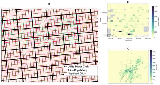
Figure 1.
(a) Map of the power grids from the utility company (large grids with grayed outlines) and the original 1 km grids (population and night light, shown as population density in red) used for model development in this study. (b) An example of accumulated power outages (customers without power) during Hurricane Katrina within the utility company grids. (c) Population density in 2005 within the 1 km grids.
There are spatial mismatches between the resolution of the utility power outage data and the 1 km population/DMSP data. Therefore, we upscaled the 1 km DMSP light data and the GPWv4 population data to the utility grid (boxes with grayed outlines in Figure 1). We calculated the population (POP in Table 1) for each utility grid by summing all 1 km population grids fully or partially contained (weighed by area) within it. We calculated the mean of the infrared radiation (MTIR), the visible light observation (MVIS), the lunar illuminance (MLI), and the standard deviations of the visible light observation (SVIS) for all cloud-free pixels within each utility grid. We applied the original cloud masks from the DMSP-OLS data to identify cloud-free pixels and used them exclusively in our power outage modeling. We also acquired the annual stabilized night light (FNL) and the detection ratio (PNL) for each pixel from the Earth Observation Group at the Colorado School of Mines (https://eogdata.mines.edu/products/dmsp/, accessed on 4 July 2024). The hurricane night visible light ratio in the annual stabilized night (VSR) is defined as MVIS/FNL, and the difference (VSD) is defined as FNL—MVIS for each pixel. Finally, we also determined the latitude (LAT) and longitude (LON) of the centroid of each utility grid and included them in the ML models. Details about the response and feature variables for our machine learning models are listed in Table 1.

Table 1.
Variables used in machine learning models.
2.2. Cloud and Data Availability
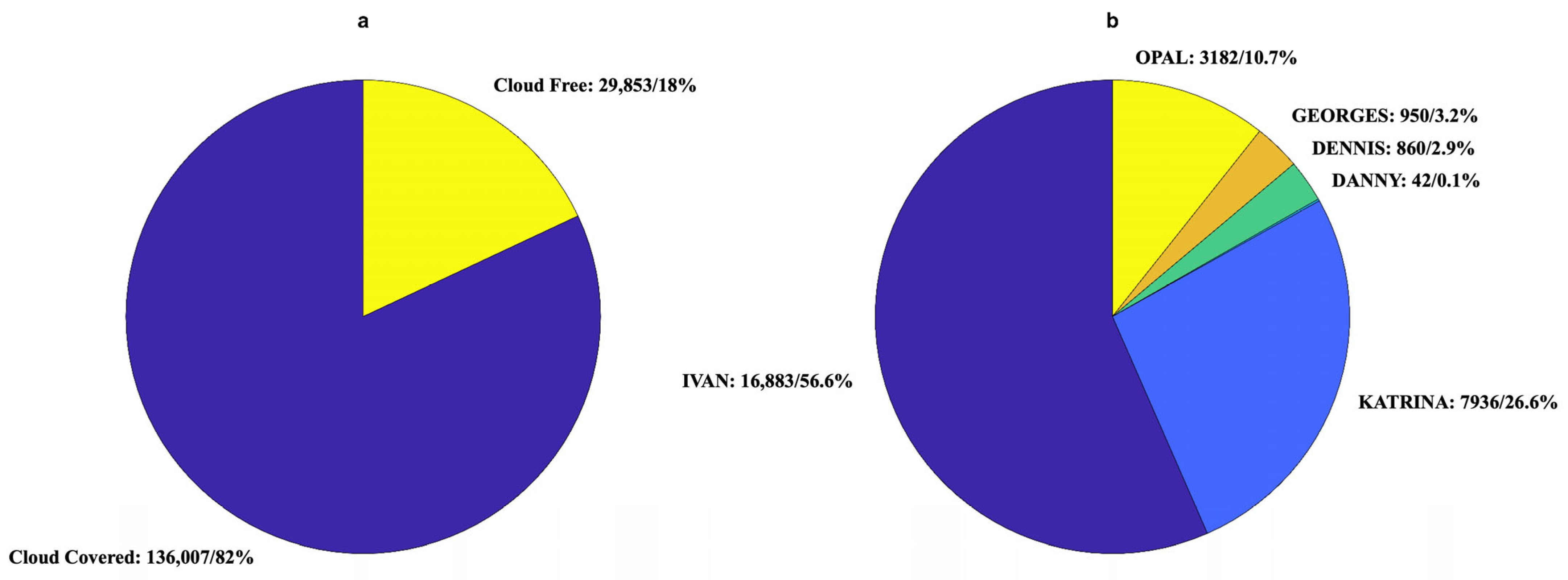
Clouds prevent the visible light signal from being detected by satellite sensors. Therefore, dealing with cloud cover is the most challenging part of using satellite night light data to detect power outages. Here, we used the primary cloud mask (a more stringent cloud mask defined by the original DMSP data) to filter out all pixels covered by clouds before averaging their values into the utility power grid. We only retained power grids with coverage of more than 90% cloud-free DMSP-OLS pixels, resulting in a total of 29,793 records (Figure 2a) for training and testing the machine learning (ML) model. Those cloud-free locations match 18% of power outage observations from 6 hurricanes. Different hurricanes vary in the shares of available observations (Figure 2b). There are 5258 power grids (21.2%) with non-zero power outages (Figure S1), and three hurricanes—Ivan, Katrina, and Opal—account for ~98% of them. The availability of cloud-free observations from each hurricane is controlled by its physical characteristics, such as size and translation speed. For example, hurricanes with larger sizes and slower translation speeds are likely to block night light detection for a location for longer due to the thick clouds associated with their deep convection.
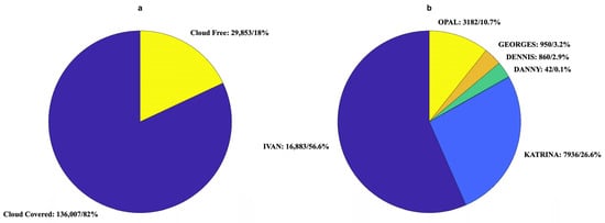
Figure 2.
(a) Number/percentage of cloud-covered and cloud-free power grids on all nights with satellite observations. (b) Number/percentage of cloud-free power grids from each hurricane used for model training/testing.
2.3. Model Overview
After data pre-processing, as shown in Figure 3, we trained and compared different machine learning (ML) models using the refined power outage data and feature variables. We evaluated four machine learning (ML) models, individually and in combination: convolutional neural networks (CNNs), a logistic model (LOG), random forest (RF), and extreme gradient boosting trees (XGBoost: XGB). Deep Learning is a widely used AI technique in remote sensing [30,31], which is constructed from the CNN algorithm based on multiple layers of a feedforward network for prediction. We leveraged the R packages “keras” [32] and “tensor” [33] to train our CNN models and make predictions. The logistic algorithm uses the generalized linear regression framework for binary classification tasks. It has been widely used to detect changes in remotely sensed imagery. RF and XGB are regression and classification tree-based algorithms. The regression/classification tree splits the data based on a feature and a threshold to reduce the variance created by each split in the subset. This recursive binary splitting continues until a minimum number of observations is reached in a leaf or a minimum reduction in variance, and new predictions involve navigating down the tree based on the feature values of the new instance until reaching a leaf node [34]. These decision tree-based models are non-parametric ML algorithms with less stringent requirements for data types and distributions. They demonstrated strong performance in predicting power outages [20]. While the RF trains many trees by bagging them into randomly selected ensembles, the XGB model builds trees one at a time and continuously builds new trees to correct bias in previously trained trees [35,36]. We used the R packages (v4.3.3) “caret” [37], “ggplot2” [38], “ISLR” [39], “randomForest” [40], and “xgboost” [41] to streamline the model training and testing processes for LOG, RF, and XGB models.
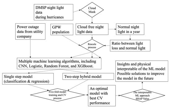
Figure 3.
Flowchart of the technical process for this study.
2.4. Model Training, Cross-Validation, and Evaluation
We developed and evaluated one-step models and hybrid models. The one-step model employs a single model to predict whether (binary) or how many (regression) power outages will occur in each power grid. LOG is the only binary model; CNN, RF, and XGB were trained for both binary and regression models. The hybrid models combine two models (which can be the same or different types) to handle separate tasks in two steps. The first step is determining whether power outages will occur at each power grid. Locations with power outages will be assigned a value of “1”, and locations without power outages will be assigned a “0”. We test the two-step hybrid model because previous hurricane power outage prediction models [42,43] have shown that the binary model at the first step can significantly reduce the uncertainty introduced by the zero-inflated data, which is commonly encountered in power outage observations. All non-zero locations will proceed to the second step, which utilizes a regression model to predict the number of power outages that are expected to occur. We have 4 binary classification models and 3 regression models, so there are 4 × 3 = 12 possible combinations for hybrid models.
We repeated the training process five times for each model, using 80% of the data as the training sample and 20% as the testing sample for evaluating out-of-sample prediction performance. We assessed the accuracy of all binary classification models as the ratio of the number of correctly predicted records in the testing sample data. Metrics for regression models and hybrid models include the mean absolute error (MAE), root mean squared error (RMSE), and the coefficient of determination (R2). We compared these performance metrics across all the models we trained and different hurricanes.
2.5. Model Interpretations
One of the major challenges for machine learning (ML) algorithms is model interpretation. We applied the SHapley Additive exPlanations (SHAP) value method to interpret the optimal model [44]. The SHAP method is based on the concept of Shapley values in game theory, which can be mathematically defined as:
Here, S represents a subset of the p features the model utilizes, and x is the feature value vector of the instance under study. vx(S) denotes the prediction for feature values in set S, marginalized over features outside of set S. In general, the SHAP value quantifies the contribution of each feature to the prediction of a specific instance relative to the average prediction across all cases. The exact SHAP value calculation is computationally demanding, so Strumbelj et al. [45] introduced the Monte-Carlo Sampling approach to approximate the exact SHAP value with much less computational demand. We calculated the SHAP values using the “shapviz” R package to evaluate feature importance and identify how individual features influence power outages in our ML models.
3. Results
3.1. Binary Models
We first tested four types of binary models that are used to predict whether any power outage will occur (1) or not (0) using 29,793 cloud-free records. Most ML models show reasonable out-of-sample performance (Table 2). XGB consistently demonstrates the best performance in the 5-fold cross-validation, with the highest accuracy, F1 Score, and AUC-ROC. XGB exhibits the best stability among all models, with the lowest standard deviations in all error metrics in all four binary models we have tested. The recall and precision analysis reveals similar results as other error statistic metrics. The confusion matrix statistics demonstrate that the LOG model has significantly lower True Positive and False Positive cases, indicating its conservative manner in predicting power outages, with a slightly larger True Negative number too. But the LOG model also has a relatively larger False Negative number when compared with other models. XGB correctly predicts most cases of power outages and the third-largest number of zero power outages, with a reasonably small number of False Positive cases and the lowest number of False Negative cases.
Table 2.
Summary of error statistics for the binary model in 5-fold cross-validation.
3.2. One-Step Regression Models
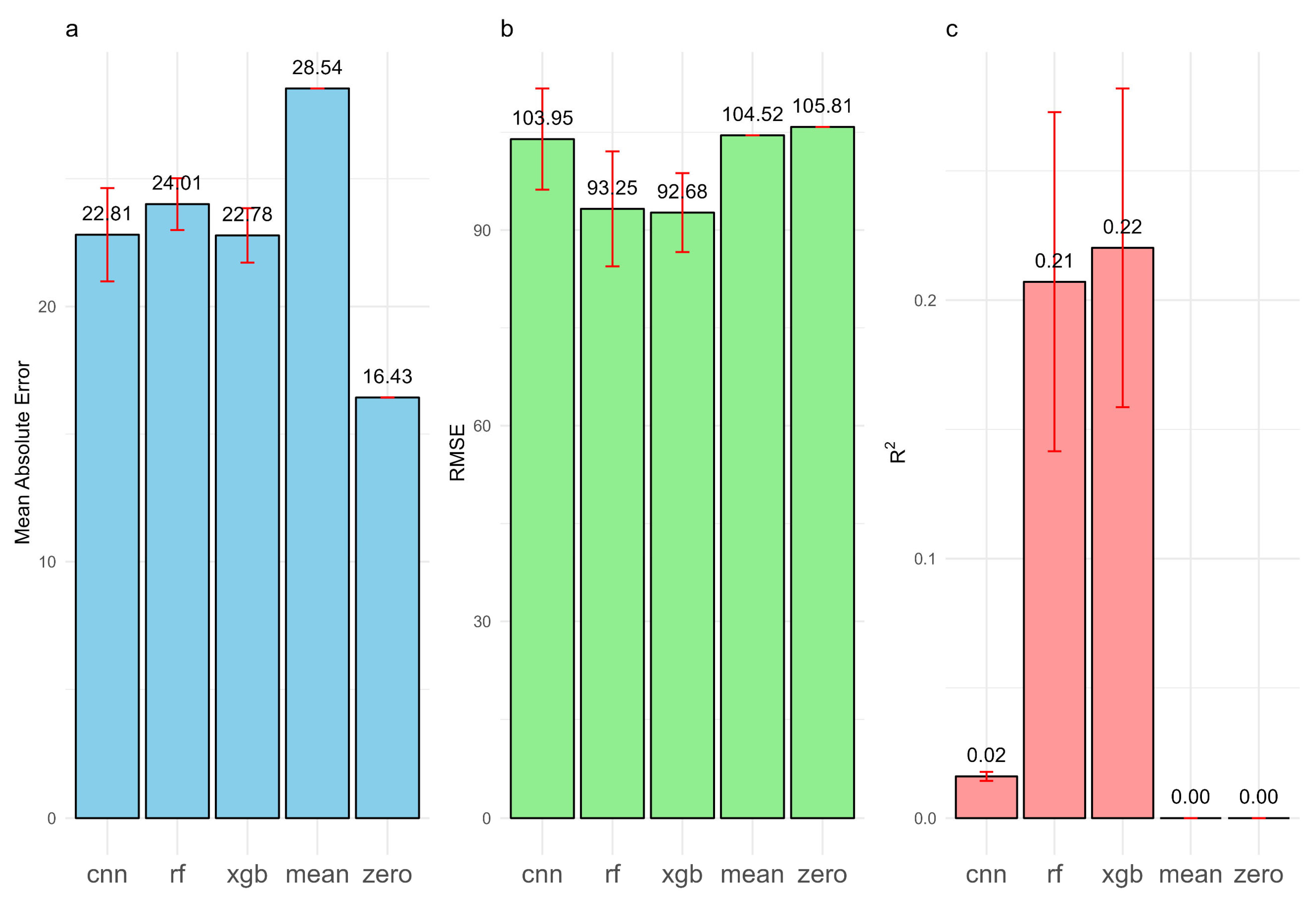
We then compared three regression models, fitting 29,793 cloud-free records directly, using the same five-fold cross-validation setup. There are large variations in prediction error metrics between different models (Figure 4 and Table S1). XGB has the lowest MAE (22.78), RMSE (92.68), and relative MAE (138%, calculated as MAE/Sample Mean), as well as the highest R2 (0.22), indicating the best and most stable performance among all three models. RF has the second-best performance, with error metrics comparable to those of XGB. Surprisingly, CNN’s R2 (0.02) is much lower than that of the other two models (by ~90%). This low performance is likely because power outage data are zero-inflated, meaning that many power grids recorded zero power outages. CNN struggles to capture this and, therefore, explains very little of the variance in the data (low R2), even though the MAE and RMSE (Figure 4a,b) are not dramatically lower than those of XGB and RF. To benchmark the performance of all models, we created two additional “no skill” models: 1. The MEAN model predicts all records as the observed sample mean power outage (16.43). 2. The ZERO model predicts that all grids will have zero power outages. The MEAN model has the highest MAE (28.54) among all models. The ZERO model has the lowest MAE (16.43) but the highest RMSE (105.81), indicating that our data is zero-inflated. The CNN model exhibits good MAE performance but does not necessarily demonstrate strong prediction performance. Our best one-step XGB model achieves 27.74% lower MAE than the MEAN model and 12.4% lower RMSE than the ZERO model.

Figure 4.
Metrics of out-of-sample prediction performance for three regression models (convolutional neural networks (CNNs), random forest (RF), and extreme gradient boosting (XGB)), the mean model (MEAN, predicting all observations as sample mean), the zero model (ZERO, predicting all observations as zero). (a) Mean absolute error (MAE), (b) root mean square error (RMSE), and (c) R2. The bar length represents the mean value calculated from five hold-out tests (with the value labeled on top of each bar), and the error bar represents the standard deviation of estimations across five hold-out tests.
3.3. Two-Step Models
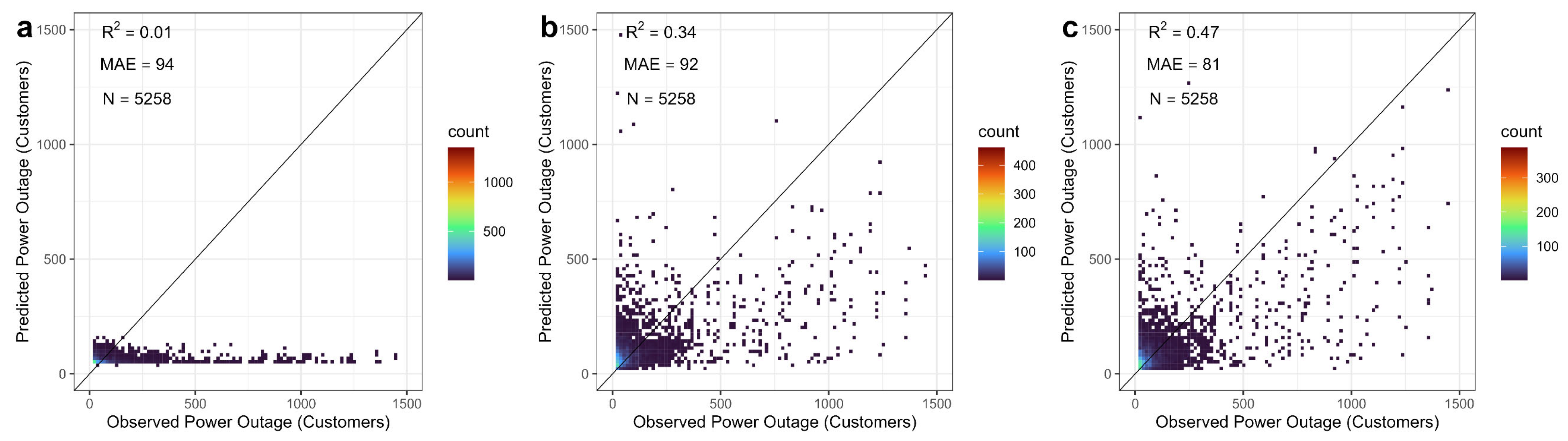
The performance of one-step regression models in Section 3.3 is heavily influenced by the large number of zero observations, which are defined as outages < 1 here and account for ~82.3% of the total cloud-free sample (Figure S1). This zero-inflation effect is most evident for CNN. However, it also influences the performance of XGB and RF. To mitigate this zero-inflation issue, we developed a series of hybrid models. The hybrid model involves two steps: (1) a binary model (developed in Section 3.2) that predicts whether power outages will occur in each grid, and (2) a regression model that predicts how many power outages will occur in locations with non-zero power outages identified from the first step. We developed three regression models (CNN, RF, and XGB) only using records with non-zero power outages. Figure 5 shows the model prediction performance for the five cross-validation folds, using non-zero power outage records selected from the same folds as in the previous analysis. There are 5258 non-zero power outage records. We can observe significant improvements in R2 in RF (by 0.13 and 62%; Figure 5b) and in XGB (by 0.25 and 114%; Figure 5c) as compared with the one-step RF and XGB models trained with all locations (Figure 4c). So the regression models perform better when only considering locations with power outages. The XGB model still exhibits the best prediction performance among all three non-zero models, with an MAE of 81 and a relative MAE of 87%. The MAE in the non-zero XGB models increased by 255% compared to the XGB model using all records (Figure 4a), which can be attributed to the larger mean of power outages from the non-zero sample (93) compared to the whole sample (16). More importantly, the relative MAE in the non-zero XGB model is 87%, which is 40% lower than that of the XGB model trained from all records, indicating an improvement in performance in the non-zero model. Compared with RF and XGB, CNN still suffers from low out-of-sample prediction accuracy due to underestimation for locations with higher power outages (Figure 5a).
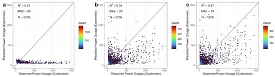
Figure 5.
Comparison of performance for different models ((a) CNN, (b) RF, and (c) XGB), trained with the data with >1 power outage in each power grid. The data are randomly divided into five hold-out testing samples and five training samples, and predictions are based solely on the testing sample data. Observations and predictions are combined from five testing samples and compared as scatter density plots with 100 equal bins. MAE and R2 are calculated based on all five testing samples.
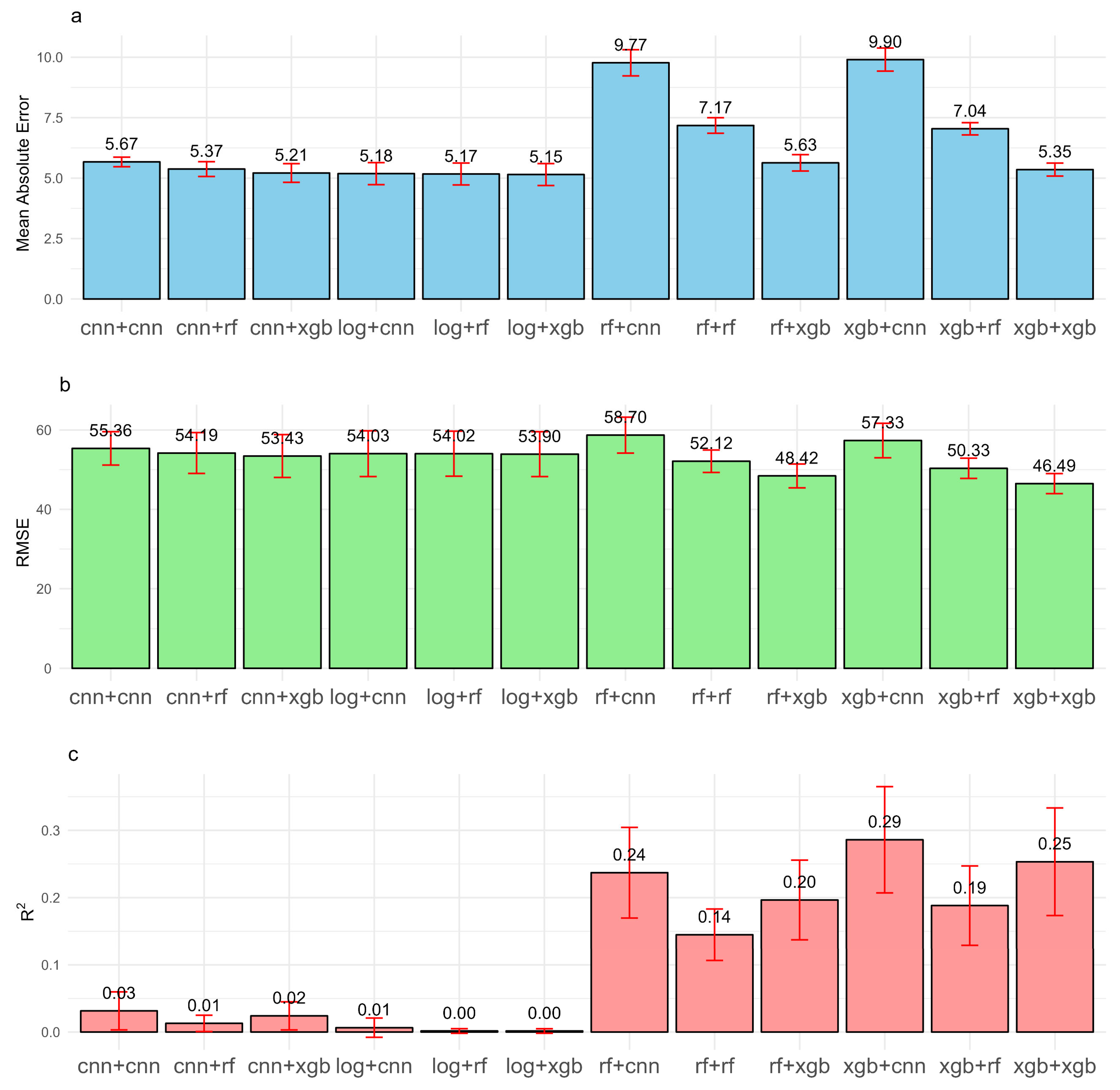
We created twelve hybrid models by iterating all possible combinations of four binary models for the first step and three regression models for the second. The results showed substantial variation in out-of-sample performance (Figure 6 and Table S2). The model with the best performance is XGB+XGB, based on all three error metrics. The XGB+XGB model exhibits further improvements over the single-step XGB model (Figure 6 vs. Figure 4), with a 76.6% reduction in mean absolute error (MAE), a 99.3% reduction in root mean square error (RMSE), and a 13.6% increase in R2. The other hybrid models also perform well, including RF+XGB, XGB+RF, and RF+RF. The better-performing models are all based on a combination of regression/classification tree algorithms. The CNN+CNN, CNN+RF, CNN+XGB, LOG+RF, LOG+XGB, and RF+CNN models have reasonable MAE (ranging from 5.15 to 5.67) and RMSE (ranging from 53.43 to 58.7), but their R2 values are very low (ranging from 0 to 0.03). The lower R2 is largely due to the low performance of binary CNN and LOG models (Table 2), where power grids with many power outages were incorrectly predicted as having no power outages. Those zero predictions reduce the MAE and RMSE metrics of the hybrid models containing CNN and LOG (Figure 6a,b), but they do not contribute to accurately predicting power outages, as reflected by their extremely low predicted explained variance (R2; Figure 6c).
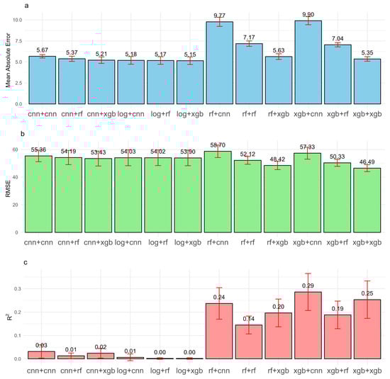
Figure 6.
Metrics of out-of-sample prediction performance for twelve hybrid models: (a) mean absolute error (MAE), (b) root mean square error (RMSE), and (c) R2. The bar length represents the mean value calculated from five hold-out tests (with the value labeled on top of each bar), and the error bar represents the standard deviation of estimations across five hold-out tests.
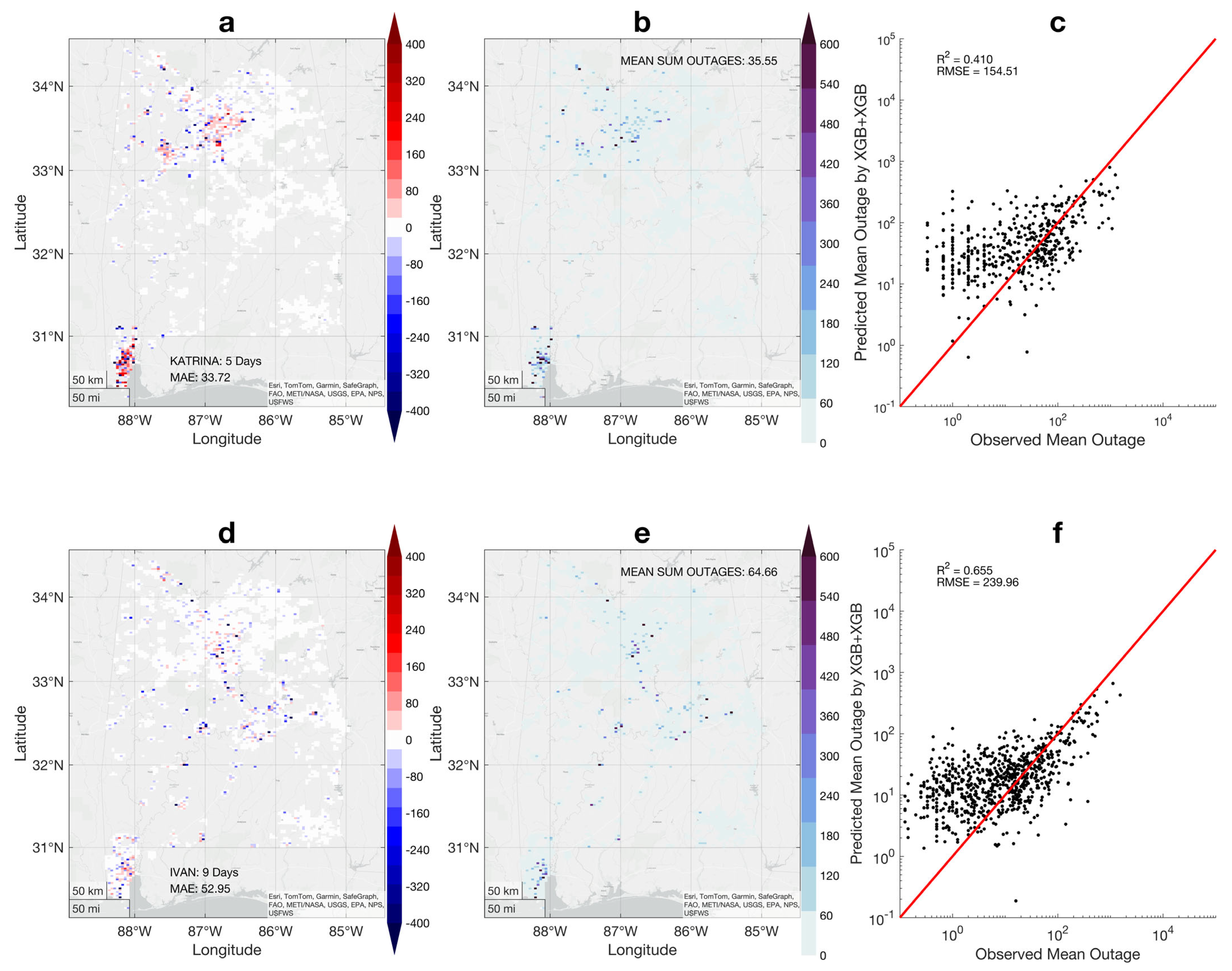
Hurricanes can vary in size, track, wind speed, and precipitation. Therefore, the spatial patterns and magnitudes of power outages may demonstrate significant variations from one hurricane to another. Here, we applied our best hybrid model (XGB+XGB) to predict the event of power outages in each hurricane by summing predictions for all nights and comparing them to the observation at each location. We compared the predictions and observations for all six hurricanes, including major hurricanes Katrina and Ivan (Figure 7), as well as the remaining four hurricanes in Figures S2 and S3. Hurricanes Katrina and Ivan demonstrate large differences in their spatial patterns of observed power outages (Figure 7b,e) and the model prediction error. For example, large overestimates are observed in the southwest corner of the study area for Hurricane Katrina (Figure 7a). In contrast, errors for Hurricane Ivan are more randomly distributed across space (Figure 7b). Overestimates are predominantly located in the lower outage range (observed power outage < 100) for both storms. Katrina and Ivan demonstrate a reasonable agreement between predictions and observations for the entire event, with R2 values of 0.41 and 0.66, respectively (Figure 7c,f). Ivan has a slightly better model performance, with a higher R2 (0.66), although its RMSE (~240) is larger due to the higher mean value of observed power outages (~65) compared to Katrina (~36). Figures S2 and S3 illustrate the model’s performance for the other four events. Hurricane Opal has both R2 and RMSE values similar to those of Ivan’s, due to its abundance of cloud-free observations. Danny, Dennis, and Georges all show very low MAE and R2, largely due to the lower availability of cloud-free non-zero observations (Figures S2 and S3b). For example, Hurricane Dennis had 860 cloud-free observations, but only 83 had non-zero power outages. The number is a very small and unstable sample compared to Hurricane Opal (Figure S3e), which had 3182 cloud-free observations and 920 non-zero power outages. Another reason for poor model performance is that some hurricanes experienced outages that mostly occurred during the daytime, and the night light data could not capture these daytime outages, particularly if they had shorter durations. For example, Hurricane Danny had 628 non-zero outages in our original record. Only 60 occurred at night when the DMSP satellite passed through with no cloud cover.
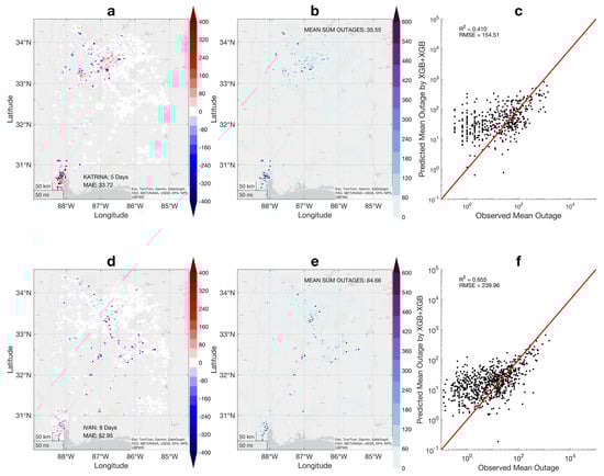
Figure 7.
Model performance for Hurricane Katrina (a–c) and Hurricane Ivan (d–f). The model errors (Observation–Prediction) are calculated for the summed power outages in each hurricane and mapped in the study area (a,d). Maps are also created for the summed power outages in each hurricane (b,e) and scatter plots between the observed and predicted summed power outages (c,f).
3.4. Model Interpretation
This section uses the SHAP value framework to interpret the XGB model for non-zero values. The SHAP value provides a systematic method for assigning importance or contribution values to individual features in a model, measuring the impact of each feature on the prediction. A positive SHAP value indicates that the feature contributes to the predicted power outages above their average. In contrast, a negative SHAP value suggests that it contributes to the predicted power outages being below their average. The absolute size of each SHAP value reflects how sensitive the predicted power outage is to that feature, revealing which features have the greatest impact. Figure 8a shows the variable importance of all 11 features used in the XGB model, calculated as the absolute mean of the SHAP value. The latitude (LAT) ranks as the most important variable in the model, and the longitude (LON) ranks as the third most important. Both location coordinate variables serve as proxies for the local information related to population, land use/land cover, vegetation, and proximity to the coast. However, it is challenging to discern the physical significance of these variables because multiple environmental and infrastructure factors are intertwined. Therefore, here we only discuss the SHAP variability for three top-ranked features that can be interpreted: the full night light (FNL, ranked fourth), the ratio of the hurricane night visible light in FNL (PNL, ranked sixth), and the population at each grid (POP, ranked second). A positive relationship exists between the SHAP value (number of power outages) and FNL (Figure 8b). Higher FNL values correspond to denser population distributions and greater numbers of electrical utility customers. Regions with more customers will have a higher probability of experiencing larger outage events when intense hurricanes occur and damage utility infrastructure. We can also identify a clear threshold when FNL is ~50. Large positive SHAP values are predominantly observed when FNL exceeds 50 and correspond to larger populations. Meanwhile, the SHAP value demonstrates a clear positive relationship with population (Figure S4b), and power grids with more than 300 people have much higher power outages. PNL reflects the amount of night light in a hurricane night compared with the stable night light from the same year [8]. Here, we can observe a clear threshold at 1 (Figure 8c), meaning that the hurricane and stable night light are equal. When PNL is less than 1, more positive SHAP values indicate that hurricane power outages are associated with losing night light. Negative SHAP values are related to PNL values larger than 1, meaning that fewer power outages are associated with less night light loss. The uncertainties in detecting hurricane night light at pixels from the DMSP cause some locations to have larger values than the annual full night light (PNL > 1). However, most of these uncertainties occur in locations with lower populations (darker blue dots on the right side of Figure 8c) and have a lesser impact on the detection accuracy of large power outage events. We can also observe a similar pattern in the SHAP plot for the VSD (Figure S4f), which indicates that positive differences (Stable−Hurricane) correspond to more positive SHAP contributions, suggesting larger outages. In summary, the DMSP night light variables play a crucial role in our ML model, and the SHAP framework can also elucidate their physical significance. The SHAP value variations for the other nine features in the XGB model are shown in Figure S4.
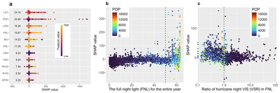
Figure 8.
The XGBoost model’s feature importance and individual relationships with power outage predictions based on the SHAP values. (a) Feature importance calculated as the SHAP value for all eleven features; (b) relationship between the full night light (FNL) and the power outage SHAP value; (c) relationship between the hurricane night visible light/FNL ratio and the power outage SHAP value.
4. Discussion
Hurricanes can cause many power outages in coastal areas. Accurate power outage predictions help emergency management organizations, NGOs, electrical utilities, and the private sector to assess power outage risks and optimize pre-storm response and preparation based on these risks. Therefore, we need accurate estimates of power outages from past storms to develop and validate TC power outage prediction models. However, power outage data are not readily available at the necessary spatial and temporal resolutions in the United States, and these data limitations are even more acute in developing countries. Therefore, we developed and evaluated algorithms to reconstruct hurricane power outage records using publicly available high-quality satellite observations of night light data and other assisting information.
We selected four classification algorithms and three regression algorithms to model power outages. Then, we rigorously tested and evaluated the performance in hold-out validations for both single-step models and hybrid models. The results show that ML models exhibit high variability in capturing power outages over the study area. The primary discovery is that the power outage data are heavily zero-inflated. The hybrid model can first predict whether power outages will occur and then estimate the number of power outages in the second step. The XGB-XGB hybrid model effectively reduced the error in predictions inflated by zero outage observations, substantially reduced the model prediction errors (RMSE) by ~100%, and increased the explained variance (R2) by 13%. The classification/regression tree-based algorithms (RF and XGB) demonstrated superior performance over the logistic and CNN models in the binary classification, and they particularly helped improve the performance of the hybrid models.
Our optimal hybrid model (XGB-XGB) also provides the best estimates of event power outages for different hurricanes. However, it tends to overestimate power outages in locations that have relatively few outages. The model also slightly underestimates the frequency of power outages at locations with a higher incidence of outages. The spatial distribution of the model predictions is random but highly correlated with the locations and magnitudes of power outage observations.
Based on the SHAP value, the interpretable ML approach provides valuable insights into ML algorithms. We found that the locations of the power grid, population, and the DMSP night light observations play crucial roles in the XGB regression model. We discovered that power outages are proportional to the population and the annual stable night light value. Power outages are sensitive to the fraction of hurricane night lights in the annual stable night light (PNL), with a larger number of power outages related to PNL values of less than 1. These results help us explain the underlying physical relationships in the ML models, which adds confidence to the predictions.
One major challenge of this approach is that hurricanes are associated with increased cloud cover. Clouds can entirely or partially block the night light from the surface [25,46]. Here, we only predicted power outages in cloud-free locations based on the cloud mask defined in the original DMSP data. Only 18% of the available locations can be used for training and validating the models because of our stringent 90% cloud-free threshold. Therefore, future research needs to test the possibility of including areas partially covered by clouds, assessing uncertainties and reliability. This could increase our ability to detect a larger proportion of power outages in the future. Another challenge to extending our current approach to global power outage estimation comes from the availability of high-quality power outage observations for model training and validation. In the United States, these observations typically originate from various sources, primarily private power companies or third-party data portals such as PowerOutage.us, and they encompass different spatial scales (or spatial aggregation units). Observations from other countries are more challenging to obtain, and the spatial scale can differ significantly from that in the United States. Therefore, future efforts should focus on developing a more general power outage estimation model that can be applied to various countries and spatial scales. One additional limitation in using the night light satellite to monitor power outages is that this technique cannot be applied to power outages with shorter durations (e.g., <12 h), particularly if they occur during the daytime. Two hurricanes in our analysis exhibited poor prediction performance in the cross-validation due to under-sampling resulting from cloud blockage or short duration.
We chose the DMSP night light data for our feature variables because the utility power outage reference data is limited to hurricanes before 2010, and the DMSP night light data is the only available source for that period. The uncertainties in the DMSP, combined with cloud cover and spatial rescaling uncertainties, could negatively impact our power outage estimation model. The VIIRS DNB data are an excellent candidate for new data, having been available since 2013. VIIRS DNB provides higher-quality data to monitor power outages caused by hurricanes and other disasters [28]. The latest data can be used to train more advanced ML models using additional hurricane cases. Larger and more reliable training data will likely enhance the model’s reliability, stability, and potential for generalization. In this study, we have tested different single-step and hybrid models using eleven potential predictors. More ML algorithms, such as the ensemble prediction approach like Bayesian model averaging (BMA), could be tested in future work to improve model performance. A more extensive set of features, such as land use, elevation, and soil characteristics, can be included in the model because those local physical characteristics can influence the probability of power outages [12,47].
5. Conclusions
To our knowledge, this is the first study to systematically evaluate the feasibility of using satellite data and ML approaches to reconstruct historical hurricane power outages based on a series of hurricanes. The findings provide a foundation for developing more generic power outage reconstruction models that cover a broader geographic area without requiring detailed information about power grid infrastructure. Those models help provide a more comprehensive dataset on the impacts of power outages from hurricanes or other natural hazards. The reconstructed dataset will provide a solid foundation for developing operational, data-driven power outage prediction models and understanding historical changes in hurricane hazard impacts. They provide essential support for global disaster mitigation and response efforts.
Supplementary Materials
The following supporting information can be downloaded at: https://www.mdpi.com/article/10.3390/rs17142347/s1, Figure S1: a. the number/fraction of power grids with (blue) and without (yellow) power outages (>1/≤1) from all cloud-free power grids; b. the number/fraction of cloud-free power grids with power outages in 6 different hurricanes; Figure S2: Model performance for individual hurricanes, Danny (a, b, c) and Dennis (d, e, f). The model errors (Observation – Prediction) are calculated for the summed power outages in each hurricane and mapped in the study area (Figures a and d). Maps are also created for the summed power outages in each hurricane (b & e), and scatter plot between the observed and predicted summed power outages (c & f); Figure S3: Model performance for individual hurricanes, Georges (a, b, c) and Opal (d, e, f). The model errors (Observation – Prediction) are calculated for the summed power outages in each hurricane and mapped in the study area (Figures a and d). Maps are also created for the summed power outages in each hurricane (b & e), and scatter plot between the observed and predicted summed power outages (c & f); Figure S4: Relationships between each feature and the SHAP value for power outages. Table S1: Metrics of out-of-sample prediction performance for three single-step regression models. Table S2: Metrics of out-of-sample prediction performance for 12 hybrid models. Table S3: Introduction of different R packages used in this study.
Author Contributions
L.Z.: Conceptualization, Methodology, Data Curation, Formal Analysis, Investigation, Writing—Original Draft, Writing—Review and Editing, and Visualization. S.M.Q.: Conceptualization, Methodology, Writing—Original Draft, Writing—Review and Editing. All authors have read and agreed to the published version of the manuscript.
Funding
This research received no external funding. The APC was funded by a special waiver from the MDPI (Multidisciplinary Digital Publishing Institute).
Data Availability Statement
All data and codes used in this study will be available upon request from the authors.
Acknowledgments
L.Z. is supported by the Support for Faculty Scholars Award from Western Michigan University and the Milton and Ruth Scherer Endowment Fund #SEF-2022-1 from the Department of Geography, Environment, and Tourism at Western Michigan University. S.M.Q. is supported by the Translational Data Analytics Institute and The Ohio State University. Some of our larger models, such as RF, were trained using parallel computing at the High-Performance Computing (HPC) facility at the Ohio Supercomputer Center (OSC).
Conflicts of Interest
The authors declare that they have no known competing financial interests or personal relationships that could have appeared to influence the work reported in this paper.
References
- Alemazkoor, N.; Rachunok, B.; Chavas, D.R.; Staid, A.; Louhghalam, A.; Nateghi, R.; Tootkaboni, M. Hurricane-induced power outage risk under climate change is primarily driven by the uncertainty in projections of future hurricane frequency. Sci. Rep. 2020, 10, 15270. [Google Scholar] [CrossRef]
- Feng, K.; Lin, N.; Gori, A.; Xi, D.; Ouyang, M.; Oppenheimer, M. Hurricane Ida’s blackout-heatwave compound risk in a changing climate. Nat. Commun. 2025, 16, 4533. [Google Scholar] [CrossRef] [PubMed]
- Rodríguez-Avellaneda, A.H.; Rodriguez, R.; Shafieezadeh, A.; Yilmaz, A. Socioeconomic disparities in hurricane-induced power outages: Insights from multi-hurricane data in Florida using XGBoost. Sustain. Cities Soc. 2025, 126, 106362. [Google Scholar] [CrossRef]
- Emanuel, K. Increasing destructiveness of tropical cyclones over the past 30 years. Nature 2005, 436, 686–688. [Google Scholar] [CrossRef]
- Emanuel, K. Global Warming Effects on U.S. Hurricane Damage. Weather Clim. Soc. 2011, 3, 261–268. [Google Scholar] [CrossRef]
- Emanuel, K. Assessing the present and future probability of Hurricane Harvey’s rainfall. Proc. Natl. Acad. Sci. USA 2017, 114, 12681–12684. [Google Scholar]
- Knutson, T.; Camargo, S.J.; Chan, J.C.L.; Emanuel, K.; Ho, C.-H.; Kossin, J.; Mohapatra, M.; Satoh, M.; Sugi, M.; Walsh, K.; et al. Tropical Cyclones and Climate Change Assessment: Part I: Detection and Attribution. Bull. Am. Meteorol. Soc. 2019, 100, 1987–2007. [Google Scholar] [CrossRef]
- Knutson, T.; Camargo, S.J.; Chan, J.C.L.; Emanuel, K.; Ho, C.-H.; Kossin, J.; Mohapatra, M.; Satoh, M.; Sugi, M.; Walsh, K.; et al. Tropical Cyclones and Climate Change Assessment: Part II: Projected Response to Anthropogenic Warming. Bull. Am. Meteorol. Soc. 2020, 101, E303–E322. [Google Scholar] [CrossRef]
- NOAA. National Centers for Environmental Information (NCEI), U.S. Billion-Dollar Weather and Climate Disasters; NOAA: Silver Spring, MD, USA, 2021.
- Yuan, S.; Quiring, S.M.; Zhu, L.; Huang, Y.; Wang, J. Development of a Typhoon Power Outage Model in Guangdong, China. Int. J. Electr. Power Energy Syst. 2020, 117, 105711. [Google Scholar] [CrossRef]
- Nateghi, R.; Guikema, S.D.; Quiring, S.M. Forecasting hurricane-induced power outage durations. Nat. Hazards 2014, 74, 1795–1811. [Google Scholar] [CrossRef]
- Quiring, S.M.; Zhu, L.; Guikema, S.D. Importance of soil and elevation characteristics for modeling hurricane-induced power outages. Nat. Hazards 2011, 58, 365–390. [Google Scholar] [CrossRef]
- Chen, H.; Yan, H.; Gong, K.; Geng, H.; Yuan, X.-C. Assessing the business interruption costs from power outages in China. Energy Econ. 2022, 105, 105757. [Google Scholar] [CrossRef]
- Cole, T.A.; Wanik, D.W.; Molthan, A.L.; Román, M.O.; Griffin, R.E. Synergistic Use of Nighttime Satellite Data, Electric Utility Infrastructure, and Ambient Population to Improve Power Outage Detections in Urban Areas. Remote Sens. 2017, 9, 286. [Google Scholar]
- Cui, H.; Qiu, S.; Wang, Y.; Zhang, Y.; Liu, Z.; Karila, K.; Jia, J.; Chen, Y. Disaster-Caused Power Outage Detection at Night Using VIIRS DNB Images. Remote Sens. 2023, 15, 640. [Google Scholar]
- Han, S.R.; Guikema, S.D.; Quiring, S.M.; Lee, K.H.; Rosowsky, D.; Davidson, R.A. Estimating the spatial distribution of power outages during hurricanes in the Gulf coast region. Reliab. Eng. Syst. Saf. 2009, 94, 199–210. [Google Scholar] [CrossRef]
- Nateghi, R.; Guikema, S.D.; Quiring, S.M. Comparison and Validation of Statistical Methods for Predicting Power Outage Durations in the Event of Hurricanes. Risk Anal. 2011, 31, 1897–1906. [Google Scholar] [CrossRef]
- Meles, T.H. Impact of power outages on households in developing countries: Evidence from Ethiopia. Energy Econ. 2020, 91, 104882. [Google Scholar] [CrossRef]
- Zheng, Q.; Seto, K.C.; Zhou, Y.; You, S.; Weng, Q. Nighttime light remote sensing for urban applications: Progress, challenges, and prospects. ISPRS J. Photogramm. Remote Sens. 2023, 202, 125–141. [Google Scholar] [CrossRef]
- Elvidge, C.D.; Baugh, K.E.; Kihn, E.A.; Kroehl, H.W.; Davis, E.R. Mapping city lights with nighttime data from the DMSP operational linescan system. Photogramm. Eng. Remote Sens. 1997, 63, 727–734. [Google Scholar]
- Imhoff, M.L.; Lawrence, W.T.; Stutzer, D.C.; Elvidge, C.D. A technique for using composite DMSP/OLS "city lights" satellite data to map urban area. Remote Sens. Environ. 1997, 61, 361–370. [Google Scholar]
- Townsend, A.C.; Bruce, D.A. The use of night-time lights satellite imagery as a measure of Australia’s regional electricity consumption and population distribution. Int. J. Remote Sens. 2010, 31, 4459–4480. [Google Scholar] [CrossRef]
- Li, X.; Liu, S.S.; Jendryke, M.; Li, D.R.; Wu, C.Q. Night-Time Light Dynamics during the Iraqi Civil War. Remote Sens. 2018, 10, 19. [Google Scholar] [CrossRef]
- Li, X.; Zhan, C.; Tao, J.B.; Li, L. Long-Term Monitoring of the Impacts of Disaster on Human Activity Using DMSP/OLS Nighttime Light Data: A Case Study of the 2008 Wenchuan, China Earthquake. Remote Sens. 2018, 10, 17. [Google Scholar] [CrossRef]
- Cao, C.Y.; Shao, X.; Uprety, S. Detecting Light Outages After Severe Storms Using the S-NPP/VIIRS Day/Night Band Radiances. IEEE Geosci. Remote Sens. Lett. 2013, 10, 1582–1586. [Google Scholar] [CrossRef]
- Miller, S.D.; Straka, W.C.; Yue, J.; Seaman, C.J.; Xu, S.; Elvidge, C.D.; Hoffmann, L.; Azeem, I. THE DARK SIDE OF HURRICANE MATTHEW Unique Perspectives from the VIIRS Day/Night Band. Bull. Am. Meteorol. Soc. 2018, 99, 2561–2574. [Google Scholar] [CrossRef]
- Zhao, X.Z.; Yu, B.L.; Liu, Y.; Yao, S.J.; Lian, T.; Chen, L.J.; Yang, C.S.; Chen, Z.Q.; Wu, J.P. NPP-VIIRS DNB Daily Data in Natural Disaster Assessment: Evidence from Selected Case Studies. Remote Sens. 2018, 10, 1526. [Google Scholar] [CrossRef]
- Roman, M.O.; Wang, Z.S.; Sun, Q.S.; Kalb, V.; Miller, S.D.; Molthan, A.; Schultz, L.; Bell, J.; Stokes, E.C.; Pandey, B.; et al. NASA’s Black Marble nighttime lights product suite. Remote Sens. Environ. 2018, 210, 113–143. [Google Scholar] [CrossRef]
- Center for International Earth Science Information Network-CIESIN-Columbia University. Gridded Population of the World, Version 4 (GPWv4): Population Density; Revision 11; NASA Socioeconomic Data and Applications Center (SEDAC): Palisades, NY, USA, 2018.
- Yuan, Q.; Shen, H.; Li, T.; Li, Z.; Li, S.; Jiang, Y.; Xu, H.; Tan, W.; Yang, Q.; Wang, J.; et al. Deep learning in environmental remote sensing: Achievements and challenges. Remote Sens. Environ. 2020, 241, 111716. [Google Scholar] [CrossRef]
- Zhang, L.; Zhang, L.; Du, B. Deep Learning for Remote Sensing Data: A Technical Tutorial on the State of the Art. IEEE Geosci. Remote Sens. Mag. 2016, 4, 22–40. [Google Scholar] [CrossRef]
- Allaire, J.J.; Chollet, F. keras: R Interface to ‘Keras’. Available online: https://CRAN.R-project.org/package=keras (accessed on 4 July 2024).
- Allaire, J.J.; Tang, Y.; Zhao, Y.; Lewis, B.W. tensorflow: R Interface to ‘TensorFlow’. Available online: https://CRAN.R-project.org/package=tensorflow (accessed on 4 July 2024).
- Hastie, T.; Tibshirani, R.; Friedman, J.H. The Elements of Statistical Learning: Data Mining, Inference, and Prediction; Springer: Berlin, Germany, 2009. [Google Scholar]
- Breiman, L. Random Forests. Mach. Learn. 2001, 45, 5–32. [Google Scholar] [CrossRef]
- Chen, T.; Guestrin, C. XGBoost: A Scalable Tree Boosting System. In Proceedings of the 22nd ACM SIGKDD International Conference on Knowledge Discovery and Data Mining; Association for Computing Machinery: San Francisco, CA, USA, 2016; pp. 785–794. [Google Scholar]
- Kuhn, M. Caret: Classification and Regression Training. Available online: https://CRAN.R-project.org/package=caret (accessed on 4 July 2024).
- Wickham, H. ggplot2: Create Elegant Data Visualisations Using the Grammar of Graphics. Available online: https://CRAN.R-project.org/package=ggplot2 (accessed on 4 July 2024).
- James, G.; Witten, D.; Hastie, T.; Tibshirani, R. ISLR: Data for An Introduction to Statistical Learning with Applications in R. Available online: https://CRAN.R-project.org/package=ISLR (accessed on 4 July 2024).
- Liaw, A.; Wiener, M. randomForest: Breiman and Cutler’s Random Forests for Classification and Regression. Available online: https://CRAN.R-project.org/package=randomForest (accessed on 4 July 2024).
- Chen, T.; He, T.; Benesty, M.; Khotilovich, V.; Tang, Y.; Cho, H.; Chen, K.; Mitchell, R. xgboost: Extreme Gradient Boosting. Available online: https://CRAN.R-project.org/package=xgboost (accessed on 4 July 2024).
- Guikema, S.D.; Quiring, S.M. Hybrid data mining-regression for infrastructure risk assessment based on zero-inflated data. Reliab. Eng. Syst. Saf. 2012, 99, 178–182. [Google Scholar] [CrossRef]
- McRoberts, D.B.; Quiring, S.M.; Guikema, S.D. Improving Hurricane Power Outage Prediction Models Through the Inclusion of Local Environmental Factors. Risk Anal. 2018, 38, 2722–2737. [Google Scholar] [CrossRef] [PubMed]
- Chen, H.; Covert, I.C.; Lundberg, S.M.; Lee, S.-I. Algorithms to estimate Shapley value feature attributions. Nat. Mach. Intell. 2023, 5, 590–601. [Google Scholar] [CrossRef]
- Štrumbelj, E.; Kononenko, I. Explaining prediction models and individual predictions with feature contributions. Knowl. Inf. Syst. 2014, 41, 647–665. [Google Scholar] [CrossRef]
- de Beurs, K.M.; McThompson, N.S.; Owsley, B.C.; Henebry, G.M. Hurricane damage detection on four major Caribbean islands. Remote Sens. Environ. 2019, 229, 1–13. [Google Scholar] [CrossRef]
- Wanik, D.W.; Anagnostou, E.N.; Hartman, B.M.; Frediani, M.E.B.; Astitha, M. Storm outage modeling for an electric distribution network in Northeastern USA. Nat. Hazards 2015, 79, 1359–1384. [Google Scholar] [CrossRef]


Disclaimer/Publisher’s Note: The statements, opinions and data contained in all publications are solely those of the individual author(s) and contributor(s) and not of MDPI and/or the editor(s). MDPI and/or the editor(s) disclaim responsibility for any injury to people or property resulting from any ideas, methods, instructions or products referred to in the content. |
© 2025 by the authors. Licensee MDPI, Basel, Switzerland. This article is an open access article distributed under the terms and conditions of the Creative Commons Attribution (CC BY) license (https://creativecommons.org/licenses/by/4.0/).