Phenology-Aware Transformer for Semantic Segmentation of Non-Food Crops from Multi-Source Remote Sensing Time Series

Abstract

Accurate identification of non-food crops underpins food security by clarifying land-use dynamics, promoting sustainable farming, and guiding efficient resource allocation. Proper identification and management maintain the balance between food and non-food cropping, a prerequisite for ecological sustainability and a healthy agricultural economy. Distinguishing large-scale non-food crops—such as oilseed rape, tea, and cotton—remains challenging because their canopy reflectance spectra are similar. This study proposes a novel phenology-aware Vision Transformer Model (PVM) for accurate, large-scale non-food crop classification. PVM incorporates a Phenology-Aware Module (PAM) that fuses multi-source remote-sensing time series with crop-growth calendars. The study area is Hunan Province, China. We collected Sentinel-1 SAR and Sentinel-2 optical imagery (2021–2022) and corresponding ground-truth samples of non-food crops. The model uses a Vision Transformer (ViT) backbone integrated with PAM. PAM dynamically adjusts temporal attention using encoded phenological cues, enabling the network to focus on key growth stages. A parallel Multi-Task Attention Fusion (MTAF) mechanism adaptively combines Sentinel-1 and Sentinel-2 time-series data. The fusion exploits sensor complementarity and mitigates cloud-induced data gaps. The fused spatiotemporal features feed a Transformer-based decoder that performs multi-class semantic segmentation. On the Hunan dataset, PVM achieved an F1-score of 74.84% and an IoU of 61.38%, outperforming MTAF-TST and 2D-U-Net + CLSTM baselines. Cross-regional validation on the Canadian Cropland Dataset confirmed the model’s generalizability, with an F1-score of 71.93% and an IoU of 55.94%. Ablation experiments verified the contribution of each module. Adding PAM raised IoU by 8.3%, whereas including MTAF improved recall by 8.91%. Overall, PVM effectively integrates phenological knowledge with multi-source imagery, delivering accurate and scalable non-food crop classification.

1. Introduction

Cultivated land serves as the foundation of agricultural production and is a vital resource for national food security. Due to rapid urbanization and global economic structural changes [1], the area planted with non-food crops (e.g., oilseeds, economic forests, medicinal plants) is expanding, directly causing a decrease in food crop yields. Converting cropland to non-food crops shrinks the area available for staple production, heightens food-supply risks, and intensifies ecological pressures, such as pesticide overuse, soil erosion, and biodiversity loss [2]. Precise identification of non-food crops is essential for evaluating land conversion impacts on food security, prioritizing food production, optimizing land resource allocation, and supporting ecological conservation [3]. Traditional monitoring methods, including field surveys and ground statistics, suffer from limited coverage, low efficiency, and inability to provide real-time dynamic monitoring, rendering them insufficient for current demands. In contrast, remote-sensing technology, characterized by extensive spatial coverage, frequent observations, and multi-source data integration, is increasingly an effective tool for monitoring non-food crops.

Despite these advantages, medium-resolution sensors face significant limitations. Nduati et al. [4], while mapping farmland in complex urban landscapes using Landsat (30 m) and MODIS (ranging from 250 m to 1000 m), found that the spatial resolution of these sensors is insufficient for capturing fine spectral details, particularly where spectral differences between crops are subtle or planting density is high. Cloud cover and rainfall often interrupt optical acquisitions, reducing the temporal resolution required for frequent tracking of crop development. Li et al. [5] explored an enhanced Landsat-MODIS fusion dataset from 2007, combining object-based image segmentation, decision-tree classification, and targeted feature selection. They found that, despite the availability of multiple spectral bands, the low spectral resolution hindered the separability between spectrally similar crops and those at adjacent phenological stages. The Sentinel-2 (S2) mission, launched in 2017, offers 10 m spatial resolution and a five-day revisit cycle, enabling finer and more frequent crop monitoring. The inclusion of red-edge bands in S2 significantly enhances the ability to distinguish subtle spectral differences between crop species. Song et al. [6] evaluated Landsat 7/8, Sentinel-2, Sentinel-1 (S1), and MODIS for mapping maize and soybean in the United States, finding that red-edge bands, sensitive to chlorophyll content and plant health, effectively differentiate healthy from stressed vegetation. However, despite the high revisit frequency of Sentinel-2, its optical sensors remain vulnerable to cloud interference, limiting all-weather observations. In contrast, Sentinel-1’s synthetic-aperture radar offers all-weather, day-and-night imaging, which is highly sensitive to crop moisture and structural characteristics, making S1 data a critical complement to optical imagery for effective crop-growth monitoring [7].

Due to the data acquisition costs and scale limitations, Sentinel-2 (S2) imagery is widely employed in traditional non-food crop classification methods. However, this approach may not sufficiently capture the spatiotemporal dynamics of crop growth, potentially limiting both the accuracy of classification and the generalizability of the model. To address these limitations, increasing the temporal frequency of data sampling has been recognized as an effective strategy for enhancing the model’s ability to capture crop phenology and dynamic growth stages. For example, Zhang et al. [6] used multi-temporal Sentinel-1 (S1) and Sentinel-2 imagery for crop mapping, showing that images from different growth stages provide a more comprehensive representation of crop phenology than single-date data, improving classification accuracy. However, multi-temporal data still have drawbacks. Yi et al. [8] created a 10 m resolution crop map of the Shiyang River Basin using multi-temporal S2 images from the 2019 growing season. They noted that manually selected phenological stages introduce subjectivity, and that multi-temporal snapshots fail to fully represent continuous phenological development, affecting classification precision. Therefore, analyzing denser S2 time series is a promising direction for future research. A time series refers to a sequence of remote-sensing images capturing the evolution of land surface characteristics over time. These images are processed to capture key phenological events in crop development. Denser Sentinel-2 (S2) time series offer clear advantages. Huang et al. [9] demonstrated that dynamic thresholding can extract continuous phenological signals from S2 data. However, optical images are frequently interrupted by cloud cover. These gaps still hamper classification in persistently cloudy regions, indicating the need for multi-sensor fusion. Hence, combining S2 and S1 time-series data has emerged as an effective strategy to overcome the intrinsic limitations of single-sensor time series. Valero et al. [10] demonstrated early-season crop monitoring by combining S1 and S2 time series, which improved reliability. However, the differing revisit intervals between S1 and S2 prevent perfect temporal alignment, leading to some limitations. To mitigate this, several studies have explored advanced fusion techniques. Orynbaikyzy et al. [11] proposed an S1–S2 fusion method based on random forests, which effectively integrates SAR and optical features, significantly enhancing crop-type classification accuracy. Dobrinić [12] applied machine-learning-based temporal fusion of S1 and S2 data to improve vegetation mapping, particularly in heterogeneous regions, boosting the accuracy and robustness of vegetation monitoring. However, these fusion algorithms typically rely on manual feature selection and operate in high-dimensional feature spaces, resulting in high computational costs and limited adaptability to heterogeneous data sources. Moreover, such methods often struggle with data gaps or noise, and in large-scale applications, data quality and completeness are critical to fusion efficacy. Deep-learning techniques, with their ability to automatically extract features and model complex relationships, show great potential for handling high-dimensional, multi-source remote-sensing data. However, in the context of highly diverse non-food crops exhibiting substantial phenological variability, issues, such as noise, cloud obstruction, and data incompleteness, challenge the stability and generalization of deep-learning models. Despite these advances, three issues remain insufficiently addressed. First, Moderate-resolution sensors or single-date imagery struggle to resolve spectrally similar non-food crops whose phenological signals diverge only at brief, growth-critical stages. Secondly, existing deep-learning approaches seldom exploit crop-calendar knowledge; fixed temporal windows or feature averaging dilute the discriminative phases that truly separate oilseed rape, tea and cotton. Finally, Optical-only methods are vulnerable to cloud-induced gaps, while most fusion frameworks still treat radar and optical streams as independent modalities, leaving their complementary dynamics under-utilized. These gaps hinder large-scale, fine-grained mapping of diverse non-food crops and motivate the phenology-aware, multi-modal strategy proposed in this work. In addition, despite the advantages of deep-learning-based classification in capturing the diversity of non-food crops, its performance and robustness still require further validation and optimization.

In crop mapping, deep learning—by virtue of its powerful feature-extraction and pattern-recognition capabilities—has markedly improved both the accuracy and efficiency of crop classification when processing large-scale, high-frequency remote-sensing data [13,14]. For example, Feng et al. [15] developed a deep-learning framework designed to enhance the accuracy of crop-type recognition from remote-sensing imagery. In the realm of single-crop identification, significant advances have also been reported. Li et al. [16] employed an improved DenseNet model to detect cotton-crop fields, delineate their spatial distribution within the study region, and monitor area changes; Xu et al. [17] proposed a DCM architecture incorporating an attention-mechanism LSTM network to generate high-resolution soybean-crop maps. Despite the excellent performance of single-crop models under controlled conditions, real-world agricultural monitoring must contend with multiple coexisting crops, overlapping phenological stages, and complex planting structures. Consequently, a growing body of research has shifted toward multi-crop recognition. Yu et al. [18] extracted temporal and spectral features to automatically learn discriminative signatures of maize, soybean, and other crops; Qiu et al. [19] combined Sentinel-1 radar data with multi-spectral time-series imagery to characterize cropping patterns and accurately classify paddy rice, wheat, maize, and other species. Although these studies employ advanced deep-learning techniques, most neglect the stage-specific phenological variability intrinsic to different crops. Crops exhibit pronounced spectral and temporal dynamics throughout their growth cycles, and these phase-dependent signatures are critical for accurate classification. Traditional approaches typically treat crops as static classes, thereby overlooking phenological transitions—especially during overlapping or rapid developmental stages—which can degrade classification performance [20]. For instance, Jiang et al. [21] presented an effective model for multi-crop classification using high-resolution temporal sequences, yet they noted that integrating meteorological data and phenological indicators with high-spatial-resolution Sentinel-1 and Sentinel-2 imagery could further enhance classification precision and reliability. To address this gap, recent work has begun to incorporate phenology explicitly. Nie et al. [20] demonstrated that mapping rice cultivation effectively requires selecting temporal windows corresponding to key phenological events, thereby supporting rice-planting monitoring and sustainable regional agro-ecosystem management; Tian et al. [22] introduced PSeqNet, a flexible multi-source integration network that explicitly models phenological correlations, achieving outstanding phenology-detection performance. Nevertheless, studies focusing on non-food crops remain relatively scarce, and existing multi-crop methods that incorporate phenology often rely on fixed time windows or feature averaging [23]. Non-food crops, such as rapeseed, cotton and tea, cover less than 20% of the arable land in our study region yet contribute more than 45% of its farm-gate income (Ministry of Agriculture, 2023) [24]. Their fields are typically smaller, more fragmented and phenologically overlapped with natural vegetation, making them markedly harder to discriminate in remote-sensing imagery than well-studied staple crops. Mapping these high-value but under-represented classes is therefore critical for precision-agriculture management and rural economic planning, and is the specific focus of this work [25].

In light of the above challenges, this study proposes a novel Phenology-Aware Vision Transformer Model (PVM), a phenology-aware semantic segmentation model for non-food crop classification. The model is built upon a Vision Transformer (VIT) and incorporates a Phenology-Aware Module (PAM) that leverages crop growth calendars to guide temporal attention toward phenologically significant stages. Additionally, a Multi-Task Attention Fusion (MTAF) mechanism is introduced to integrate Sentinel-1 SAR and Sentinel-2 optical time-series data, addressing cloud-induced discontinuities. This dual-modular design enables accurate, scalable classification of non-food crops with complex and variable phenological dynamics.

2. Study Area and Data

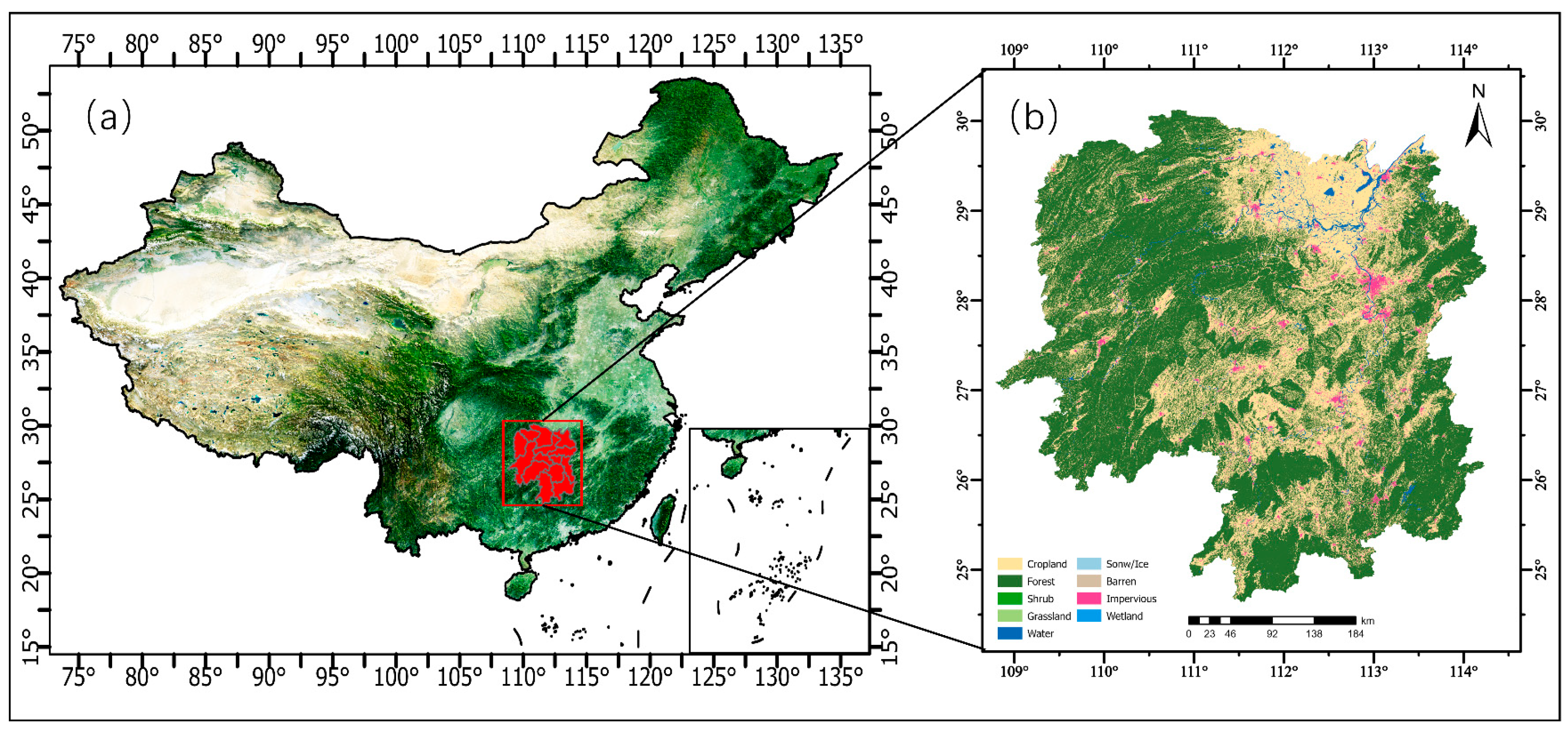
2.1. Study Area

This study selects Hunan Province, China, as the research area, focusing primarily on the typical economic crops in the province (as shown in Figure 1). Hunan Province is located in the middle reaches of the Yangtze River (108°47′E–114°15′E, 24°38′N–30°08′N), with a total area of approximately 211,800 square kilometers. The province has a subtropical monsoon climate, with an average annual temperature of 16–18 °C and annual precipitation ranging from 1200 to 1700 mm. The area of cultivated land plays a crucial role in the province’s land use, contributing significantly to food production.

Hunan is one of China’s major grain-producing bases, but in recent years, due to insufficient regulation and policy adjustments, some arable land has been converted to non-food crop cultivation, which has impacted food production and posed challenges to the efficient utilization of arable land resources.

In this context, non-food crops in Hunan, such as cotton, tea, and rapeseed, benefit from the ideal growing conditions provided by the province’s distinct four seasons and synchronized rainfall and heat. These crops were selected for this study for the following reasons: Hunan is a major production base for both rapeseed and tea, with rapeseed cultivation accounting for over 10% of the national area, and tea production ranking among the highest in China. Cotton, as a regional specialty economic crop, also holds significant economic value. Therefore, studying these non-food crops is of great importance for enhancing agricultural economic development in the region.

2.2. Data

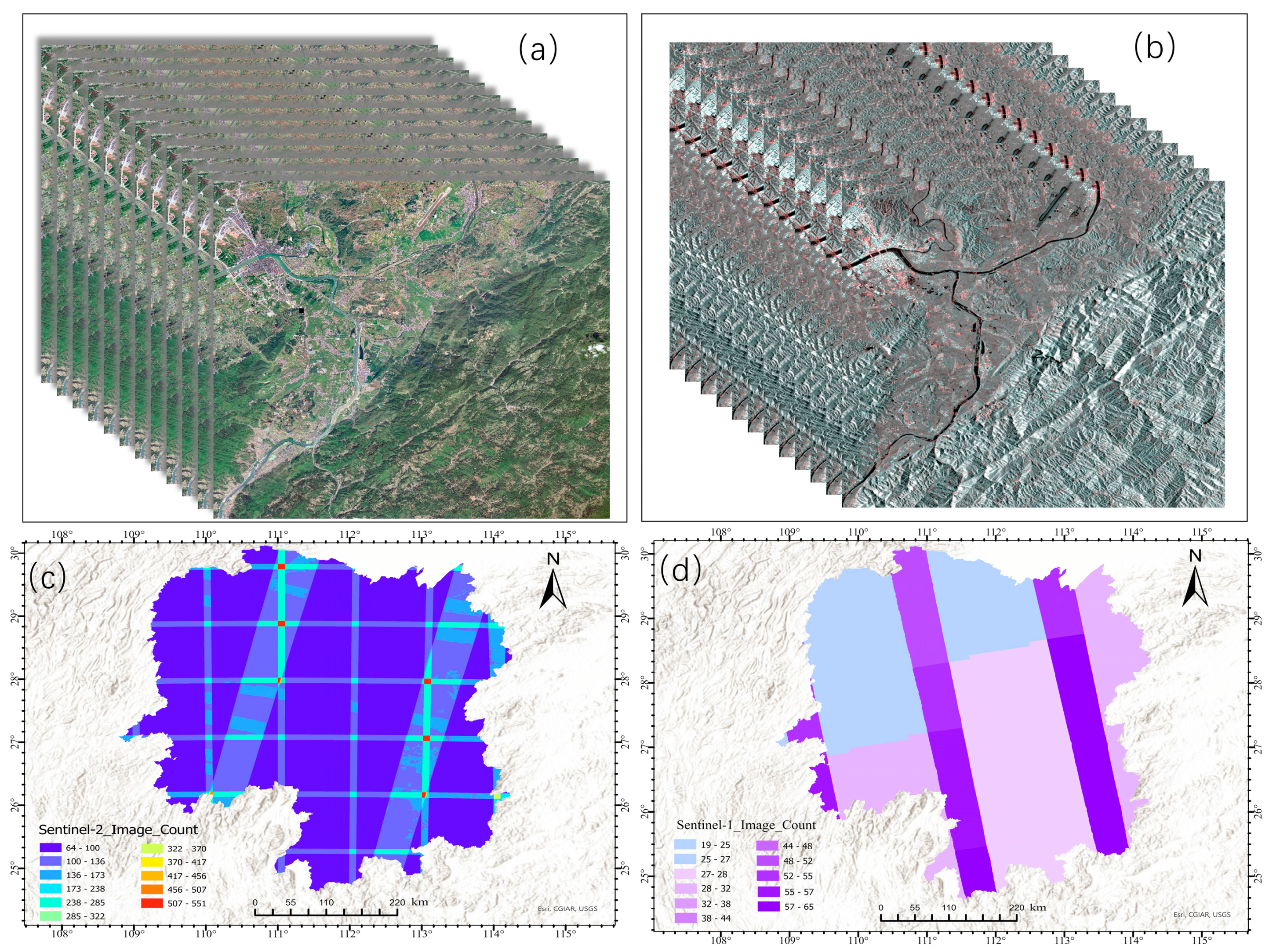
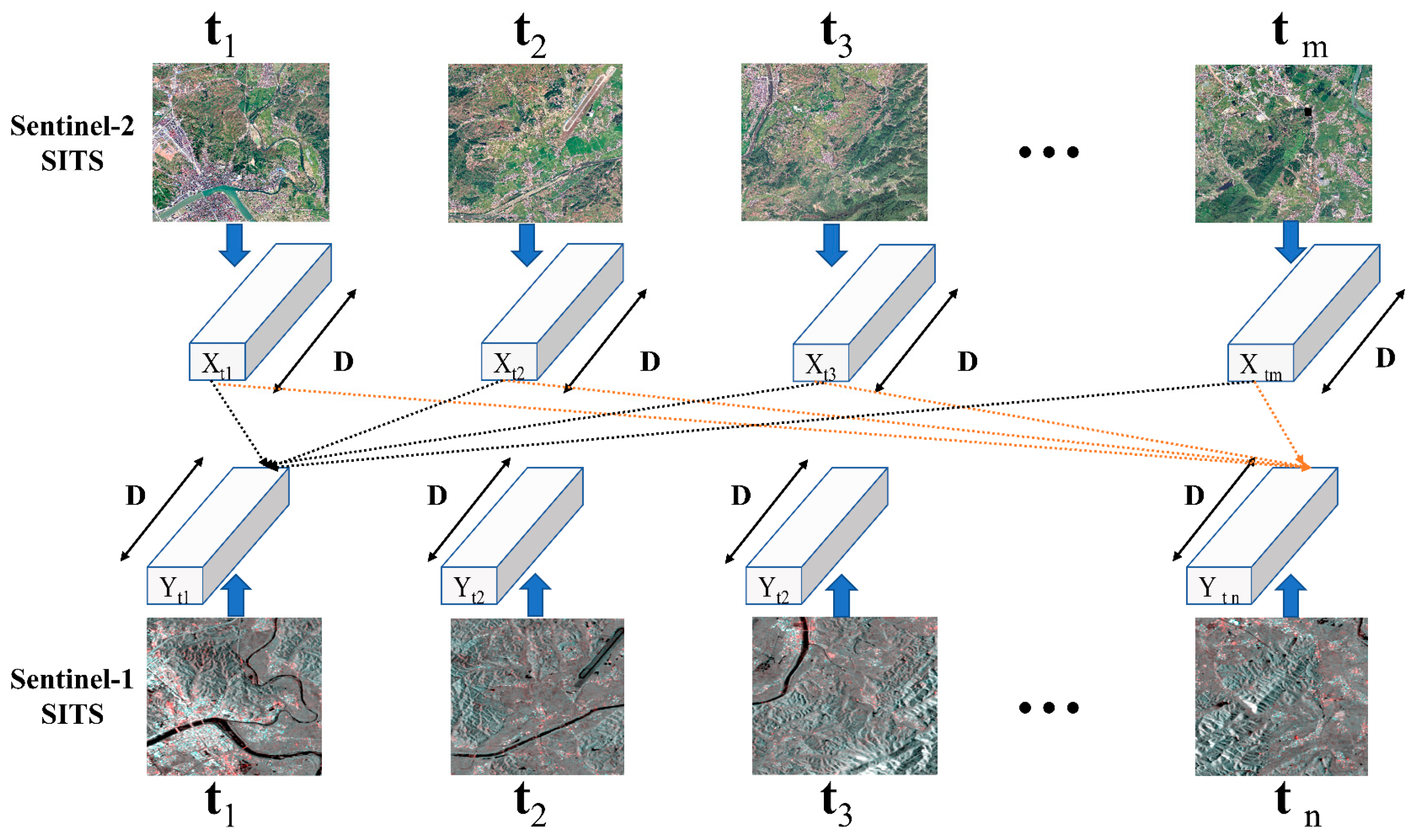
2.2.1. Remote-Sensing Data

Remote-sensing data employed in this study were acquired from the Sentinel-1 and Sentinel-2 satellite constellations via the Google Earth Engine (GEE) platform. Sentinel-2 acquisitions comprised spectral bands B2 (blue), B3 (green), B4 (red), B5 (red-edge) and B8 (near-infrared), whereas Sentinel-1 data consisted of dual-polarization SAR backscatter (VV and VH). Given that the study area (Hunan Province) experiences frequent cloud cover and precipitation—particularly during the rainy season (June–August)—the temporal availability of Sentinel-2 imagery is markedly constrained. We therefore retrieved all imagery acquired between October 2021 and October 2022, and, following a cloud-mask threshold of <70% and general quality screening in GEE, retained only those scenes meeting these criteria; no attempt was made to enforce a uniform monthly composite. As illustrated in Figure 2c, the count of usable Sentinel-2 scenes varies by month (e.g., six scenes in May, but virtually none in July and December), resulting in an intentionally irregular time series that reflects true observational conditions. In contrast, Sentinel-1 acquisitions were available consistently each month; we generated median composites on a monthly basis to produce a continuous SAR time series (Figure 2d).

For Sentinel-2 preprocessing, cloud and shadow pixels were first excluded using the QA60 band. In months with multiple valid scenes, a per-pixel median composite was computed to further mitigate cloud artefacts. Any residual data gaps in the composite images were filled via localized interpolation, and the resulting series underwent temporal smoothing using a Savitzky–Golay filter. Crucially, no artificial interpolation or gap-filling was applied across the overall temporal dimension, thereby preserving the genuine discontinuities and non-aligned structure inherent to real-world remote-sensing observations.

Due to the inherent characteristics of Sentinel-1 data (with a resolution of 10 m), particularly the speckle noise commonly found in Synthetic Aperture Radar (SAR) images, this noise interferes with the accurate representation of surface information. To address this, we applied multi-look processing and the Lee filter for speckle filtering [26]. These two methods work together to effectively reduce the noise impact and enhance image detail clarity [27]. Considering that the topographic variations in the study area might interfere with radar signals, we performed terrain correction using a Digital Elevation Model (DEM). This step eliminates distortions caused by terrain, ensuring the geometric accuracy of the data. Finally, the data were logarithmically converted to the dB scale. We chose to generate the final Sentinel-1 time-series images on a monthly basis. Specifically, for each month, we used median compositing to compute the median value for each pixel from all available Sentinel-1 images of that month. The advantages of this approach are twofold: first, it further suppresses residual noise; second, it generates stable monthly feature representations, ensuring spatial seamlessness of the data. As a result, the data for each month not only reflects true surface changes but also aligns with the crop growth cycle. To address coverage gaps caused by orbital limitations, we employed a least squares fitting method to fill missing values and applied the SG filter to smooth the time series, ensuring temporal continuity. In the end, a total of 12 Sentinel-1 time-series images were constructed.

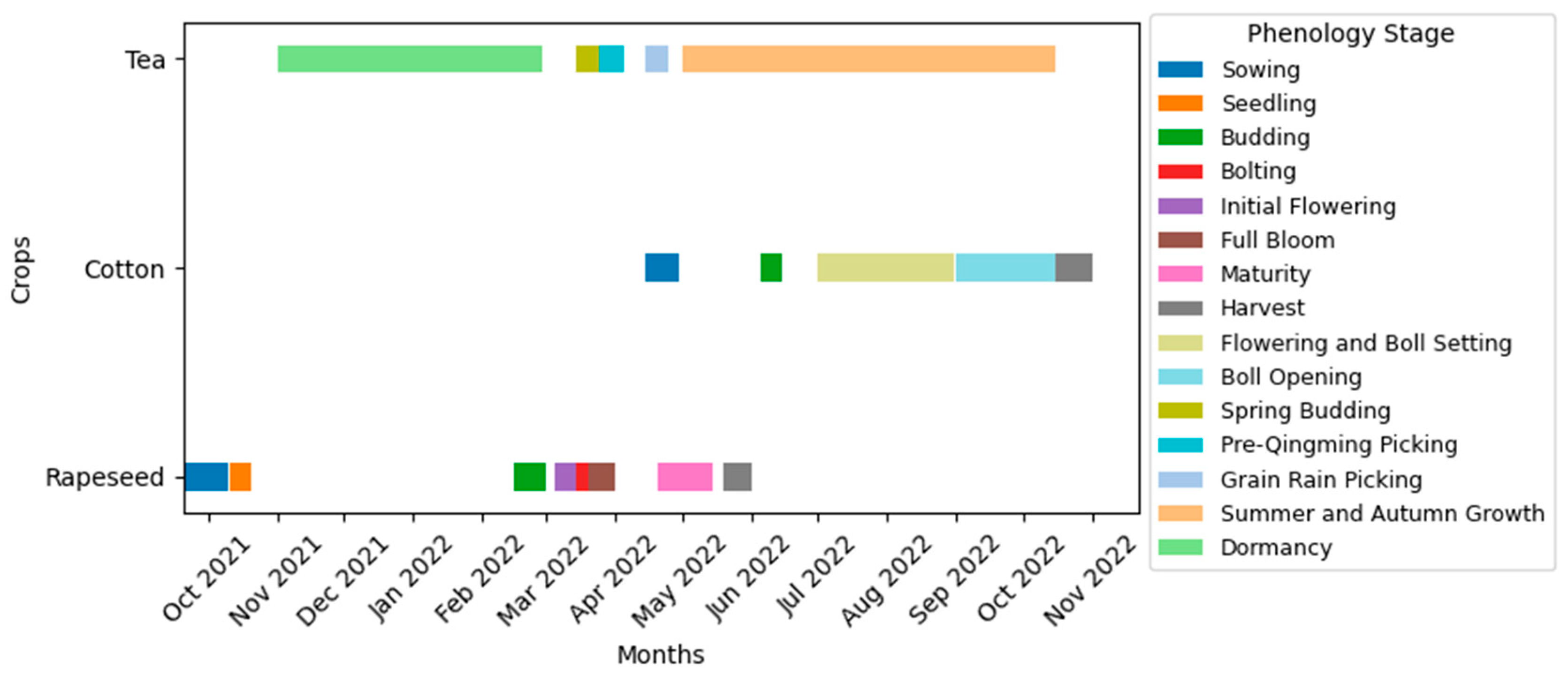
2.2.2. Auxiliary Data

This study introduces crop phenology information to enhance the model’s ability to perceive the growth cycle. Phenology data records the key growth stages of each crop and their corresponding time windows, which help the model dynamically adjust its focus at different time points, concentrating on the most distinguishing growth stages, thereby improving crop classification and multi-class semantic segmentation accuracy (as shown in Figure 3). These phenology data primarily come from the agricultural department of Hunan Province and are validated by relevant data from the Agricultural Meteorological Bureau, covering the growth stage time windows of cotton, tea, and rapeseed in 2022. These data specifically reflect the timing of various growth stages, such as sowing, green-up, heading, flowering, and maturation, providing the model with key temporal features.

Since phenology data is typically presented at discrete time points, the stage information needs to be first converted into vector form using one-hot encoding and then further mapped into a continuous feature space through linear transformation to ensure that phenology information can seamlessly integrate with other features of remote-sensing data. Furthermore, because the sampling frequencies of phenology data and remote-sensing data may differ, and phenology data often contains missing values and noise [28], linear interpolation and Savitzky–Golay (SG) filter smoothing are required to fill missing values and remove outliers, ensuring the temporal synchronization and data quality stability between phenology and remote-sensing data [29].

2.2.3. Sample Data

To ensure the accuracy of crop classification, it is crucial to guarantee the representativeness and stability of the sample data. The sample data used in this study are based on multi-year samples of three non-food crops provided by the Hunan Provincial Institute of Surveying and Mapping, combined with non-food crop planting data from the Ministry of Agriculture and Rural Affairs of China (www.moa.gov.cn). Tile-wise labeling workflow is as follows: Original vector polygons were first rasterized to a 10 m grid that matches the Sentinel-2 ground sampling distance. The entire province was then divided into non-overlapping 512 × 512-pixel tiles identical to the model input size. For each tile we calculated the proportion of pixels belonging to each crop polygon. A tile was assigned to class c only if pixels of class c covered at least 80% of its area; otherwise, the tile was excluded from training and validation. This majority-vote criterion minimizes label noise while avoiding the impractical task of per-pixel manual annotation. By overlaying and integrating both datasets, and combining with field verification conducted between October 2021 and October 2022, a total of 9990 valid samples were obtained. The data were divided as follows: 60% for training, 20% for validation, and 20% for testing. To improve the stability and generalization ability of the model, all sample data underwent strict preprocessing. First, noise and low-quality fragmented areas were removed, as remote-sensing images often contain noisy and irrelevant small fragments that can affect classification accuracy. To eliminate these interferences, spatial smoothing and texture analysis techniques were applied to remove small, irrelevant noise areas. Additionally, in terms of spatial distribution of samples, a sample balancing strategy was applied to ensure a balanced distribution of samples for each crop class in the training, validation, and testing datasets. Oversampling or undersampling methods were used to eliminate classification bias caused by class imbalance, enhancing the model’s ability to recognize minority crop classes. To further optimize data quality, the data underwent geometric correction, radiometric correction, and standardization of different sensor data to ensure that data from different platforms and time points were compared under the same standard. Furthermore, considering the different spatial and temporal resolutions of remote-sensing data, the time-series data were interpolated and smoothed to reduce the impact of inconsistent time steps or missing data. Finally, by integrating optical and radar data, this study constructed a time-series dataset for non-food crops, providing high-quality input data for subsequent semantic segmentation tasks. A total of 9990 field-verified plots, each representing one 10 m × 10 m Sentinel-2 pixel, were collected with sub-3 m RTK-GPS between October 2021 and October 2022 and then divided 60–20–20% into training (5994 plots), validation (1998) and test (1998) sets. To ensure geographic representativeness, plots were allocated in proportion to cropland area across the region’s three agro-ecological zones: 3996 plots (≈40%) lie in hilly uplands that account for 39% of cropland, 3497 plots (≈35%) in alluvial plains covering 37%, and 2497 plots (≈25%) in river-basin terrain, whose share is 24%; the deviation from perfect proportionality is therefore no greater than one percentage point in any zone. Because pixel-level statistics in

Table 1. Statistical data of the Hunan non-food crop dataset.

Label	Type	Pixels
1	Cropland	564,117,840
2	Oilseed rape	44,745,893
3	Tea	30,280,657
4	Cotton	2,537,294

show a strong class imbalance—oilseed-rape dominates while cotton is scarce—we applied a mild balancing step after the spatial draw, slightly undersampling rape parcels and oversampling independent cotton parcels, so that the final plot count is 3995 for rapeseed, 3112 for tea and 2883 for cotton. Field visits were scheduled to coincide with phenologically distinctive phases: 1541 plots were recorded in October–December 2021, 1819 in January–March 2022, 4152 in April–June 2022, and 2478 in July–October 2022. This design guarantees that every crop is observed when its spectral signature is most distinctive, gives each class a comparable number of learning samples despite the underlying pixel imbalance, and preserves the real-world spatial mosaic of the study area. To compensate for the limited number of labeled “non-food-crop” pixels in southern China and to test cross-regional generalizability, we additionally employed the 2021 Canadian Cropland Dataset (CCD). Although staples dominate the CCD as a whole, it also contains three extensive non-food categories—rapeseed, flax and alfalfa—whose spectral–phenological signatures differ from those of Chinese crops. We extracted 41,672 canola parcels, 12,534 flax parcels, and 9118 alfalfa parcels, retaining only the surrounding pixels of major crops to preserve a realistic landscape context. This experimental design enables us to assess the cross-region and cross-crop-type generalization capability of the proposed method under diverse agro-ecological conditions.

2.3. Experimental Datasets

The input dataset for this experiment comprises time-series imagery from Sentinel-1 and Sentinel-2, from which Huang et al.’s CLCD dataset [30] was used to identify cropland pixels. Based on these cropland masks, a pixel-level semantic segmentation dataset was created, containing four classes: cropland (background), rapeseed, tea, and cotton. Model training and classification were restricted to cropland regions by applying the cropland mask; pixels outside this mask were excluded from both training and inference to prevent non-cropland areas from biasing the classifier. The number of manually labeled pixels per class is summarized in Table 1. All annotation was performed in ArcGIS Pro (version 3.0) using the sample data described in Section 2. Both SAR and optical time series consist of 12 monthly time steps. To accommodate the spatial extent of the study area, the dataset was tiled into non-overlapping 512 × 512 pixel patches, uniformly distributed across the region of interest. All data products were exported in TIFF format.

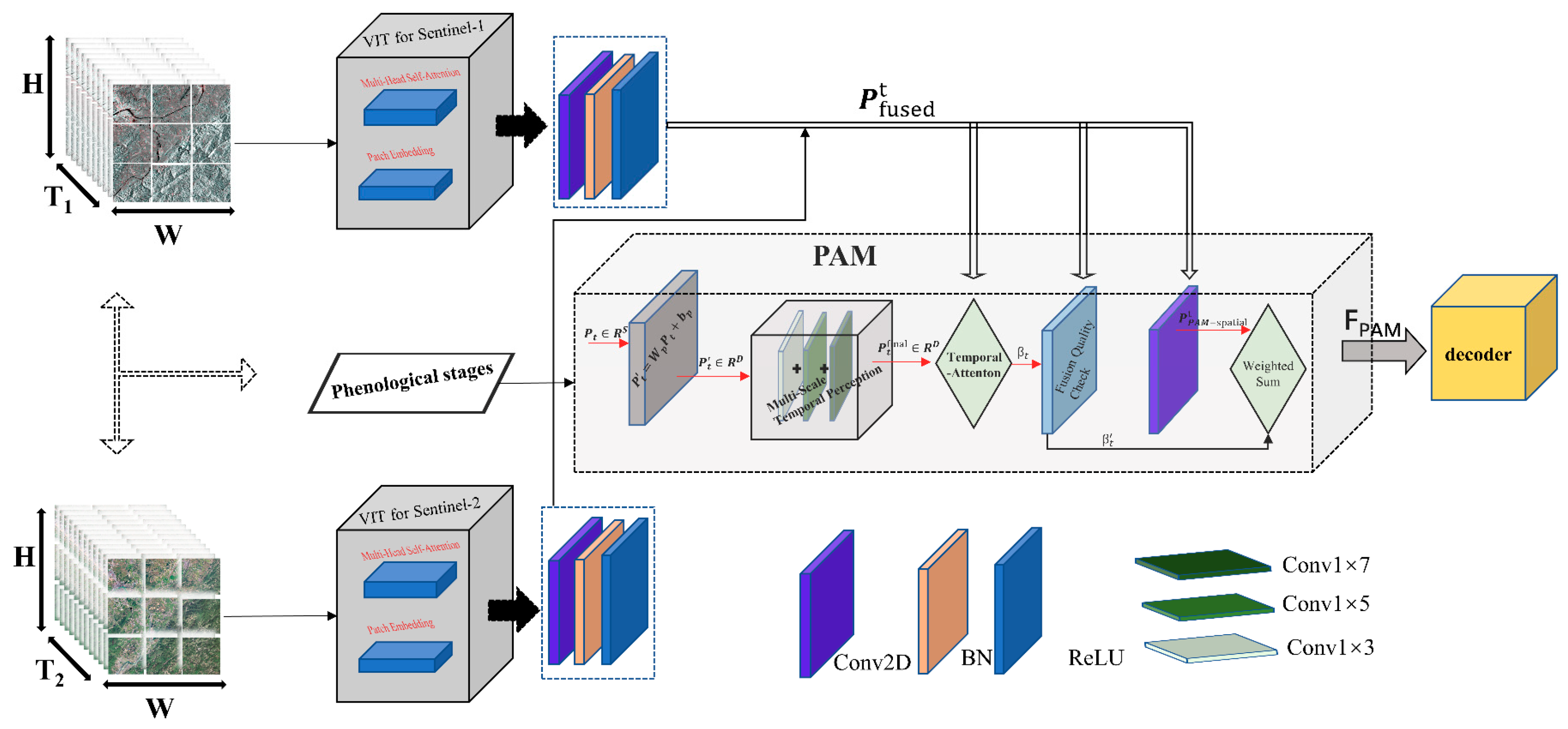
3. Materials and Methods

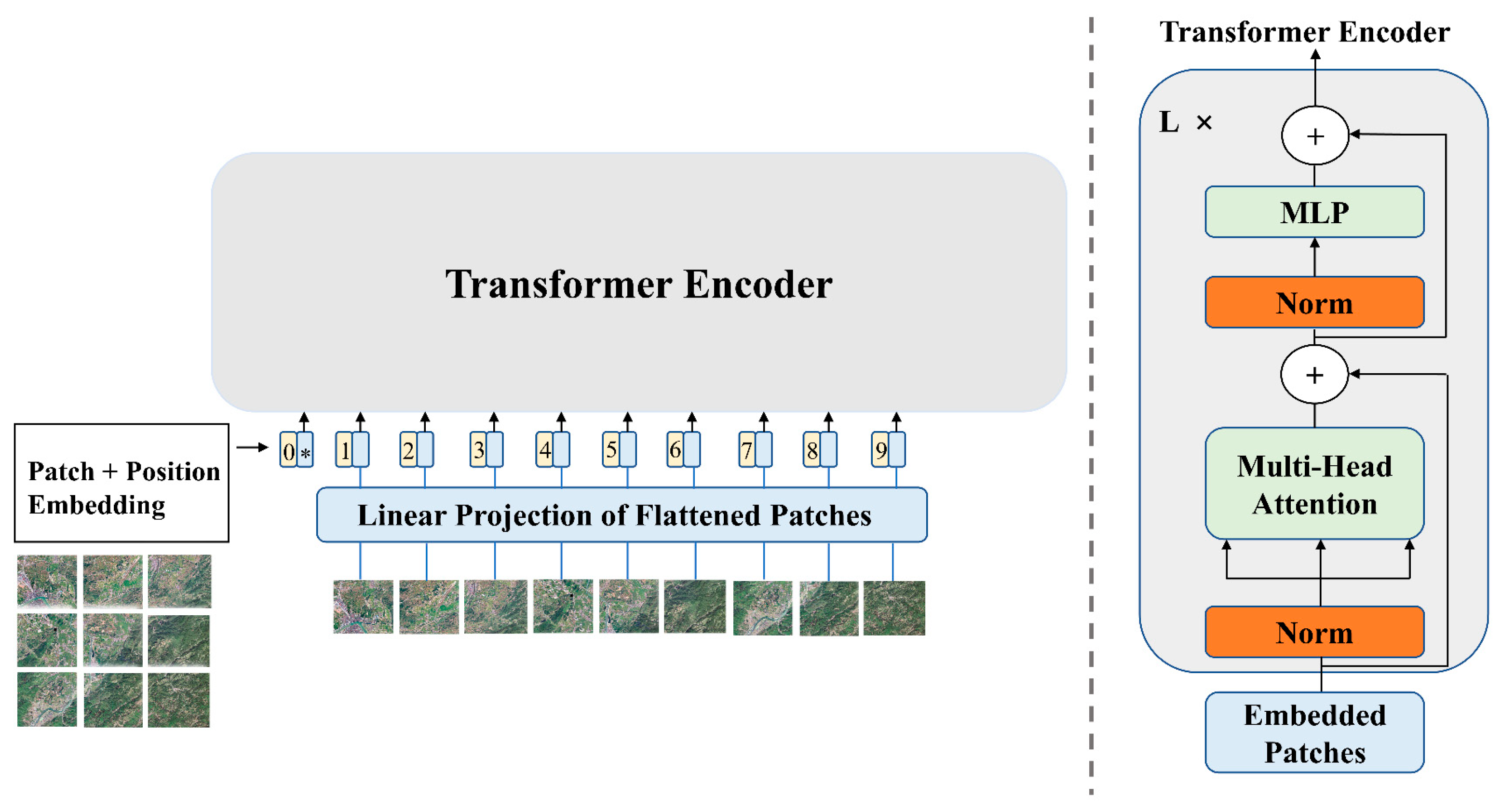
The proposed semantic segmentation network, PVM, mainly consists of an encoder, a time-series processing module, and a decoder (as shown in Figure 4). In the encoder, we employ the Vision Transformer (ViT) as the backbone to extract spatial features from the input remote-sensing images. To capture the temporal dynamics inherent in time-series data, we employed the Multi-Task Attention Fusion (MTAF) mechanism [31], which effectively integrates multi-modal and multi-temporal features. Additionally, we introduced the Phenology-Aware Module (PAM) to incorporate phenological stage information, dynamically adjusting attention to different time steps based on the crop growth cycle.

3.1. VIT Module

VIT (Vision Transformer) is an image processing model based on the Transformer architecture, first proposed by Dosovitskiy et al. in 2020 [32]. It processes image data through the self-attention mechanism, as shown in Figure 5.

Unlike traditional Convolutional Neural Networks (CNNs), VIT does not rely on convolution operations. Instead, it captures the relationships between different regions of the image by modeling global dependencies. In remote-sensing image processing tasks, VIT is capable of effectively handling high-resolution remote-sensing data, capturing spatial information and global contextual relationships. In this study, VIT is used as the encoder to extract spatial features from the input remote-sensing images. Specifically, we divide the remote-sensing images into fixed-size patches, flatten each patch into a one-dimensional vector, and apply linear projection. Then, the self-attention mechanism and feed-forward networks are used to generate feature representations. This approach allows VIT to capture global dependencies in remote-sensing images, overcoming the limitations of traditional convolutional networks when capturing large-scale features. The process is represented by the following equation (see Formulas (1)–(4)):

N = HP × WP

(1)

where P is the patch size (e.g., P = 16), and N is the total number of patches.

$$z_{\left(\left(t,i\right)\right)}=W_{\mathrm{proj}}·\mathrm{flatten}\left(x_{\left(\left(t,i\right)\right)}\right)+b_{\mathrm{proj}}$$

(2)

$$z_{\left(\left(t,i\right)\right)}^{\prime }=z_{\left(\left(t,i\right)\right)}+PE\left(i\right)$$

(3)

where $x_{\left(\left(t,i\right)\right)}$ is the flattened vector of the $i$-th patch; $W_{\mathrm{proj}}\in R^{\left(\left(D\times \left(P^{𝟚}·C\right)\right)\right)}$ is the projection weight matrix; $b_{\mathrm{proj}}\in R^D$ is the bias vector. PE($i$) is the positional encoding vector corresponding to the patch position $i$.

$$\mathrm{Attention}\left(Q,K,V\right)=\mathrm{Softmax}\left({\displaystyle \frac{\left(Q{K}^T\right)}{\sqrt{\left(\left(d_k\right)\right)}}}\right)V$$

(4)

where Q is the query matrix, K is the key matrix and V is the value matrix, all generated from the input embeddings through linear transformations. $d_k$ is the dimension of the key vector, used for scaling to prevent excessively large values.

In this study, the advantage of the VIT module lies in its ability to fully utilize the spatial information and global context in remote-sensing data, thereby enhancing its ability to recognize the growth stages and temporal changes in non-food crops. In this way, VIT not only extracts fine-grained spatial features but also increases the model’s sensitivity to the spectral characteristics of crops at different growth stages.

3.2. Multi-Task Attention Fusion (MTAF) Module

To fuse multi-modal features from Sentinel-1 and Sentinel-2 data, we introduce the Multi-Task Attention Fusion (MTAF) module proposed by Yan et al. [31] into the next stage of the VIT framework’s encoder for multi-modal feature fusion. This module uses a multi-task learning framework combined with the attention mechanism to dynamically assign weights to each modality (as shown in Figure 6). At each time step t, the MTAF module processes the feature maps $F_s{1}^t$ from Sentinel-1 and $F_s{2}^t$ from Sentinel-2. The modality-specific attention weights ${\alpha }_s{1}^t$ and ${\alpha }_s{2}^t$ are calculated through a scoring mechanism and then normalized using the Softmax function (see Formulas (5) and (6)):

$${\alpha }_s{1}^t,{\alpha }_s{2}^t=\mathrm{Softmax}\left(W_a·\mathrm{concat}\left(F_s{1}^t,F_s{2}^t\right)\right)$$

(5)

$$F_{\mathrm{fused}}^t={\alpha }_s{1}^t·F_s{1}^t+{\alpha }_s{2}^t·F_s{2}^t$$

(6)

where $W_a$ is the learnable parameter matrix, and “$concat$” represents feature concatenation. The fused feature map is obtained through a weighted combination.

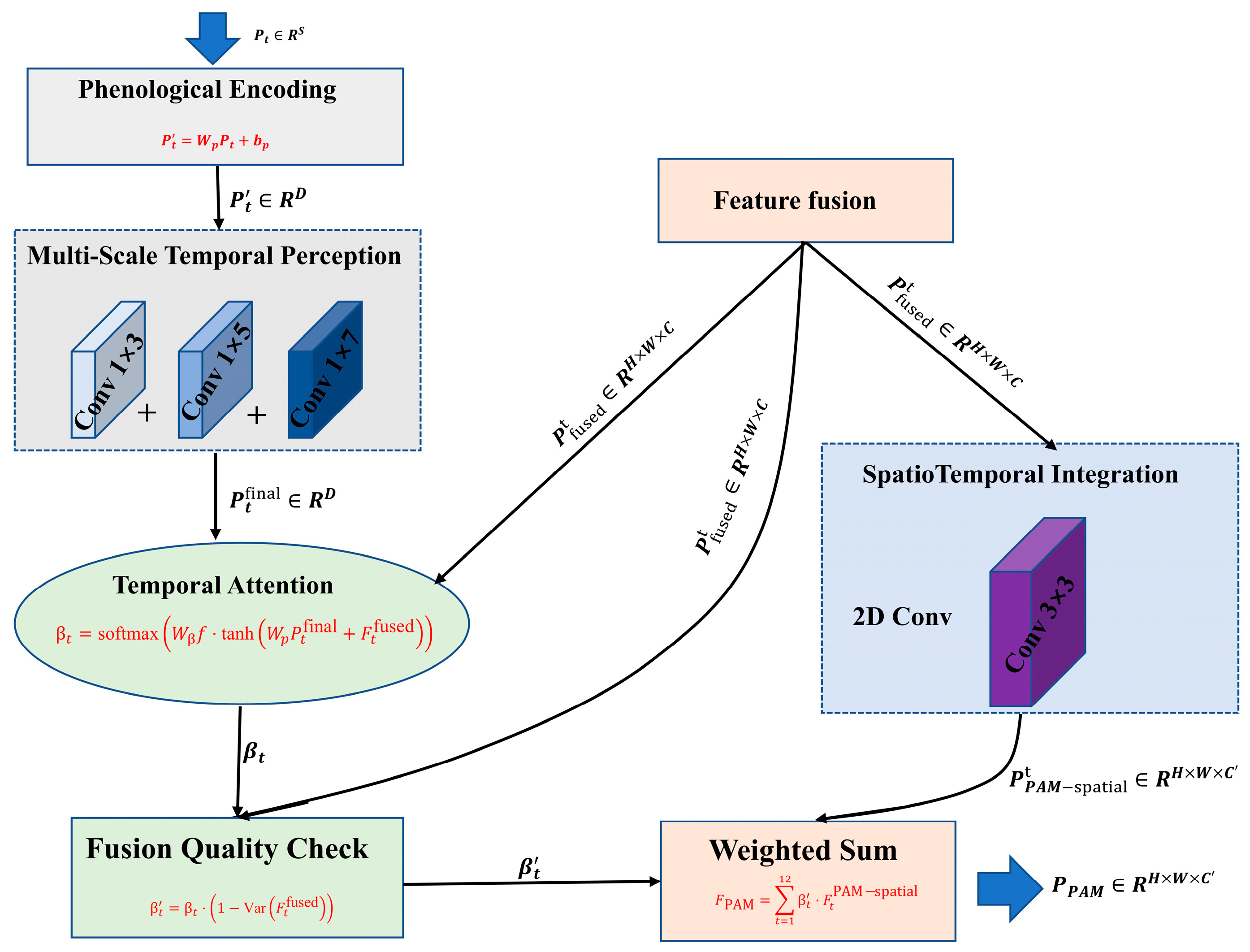
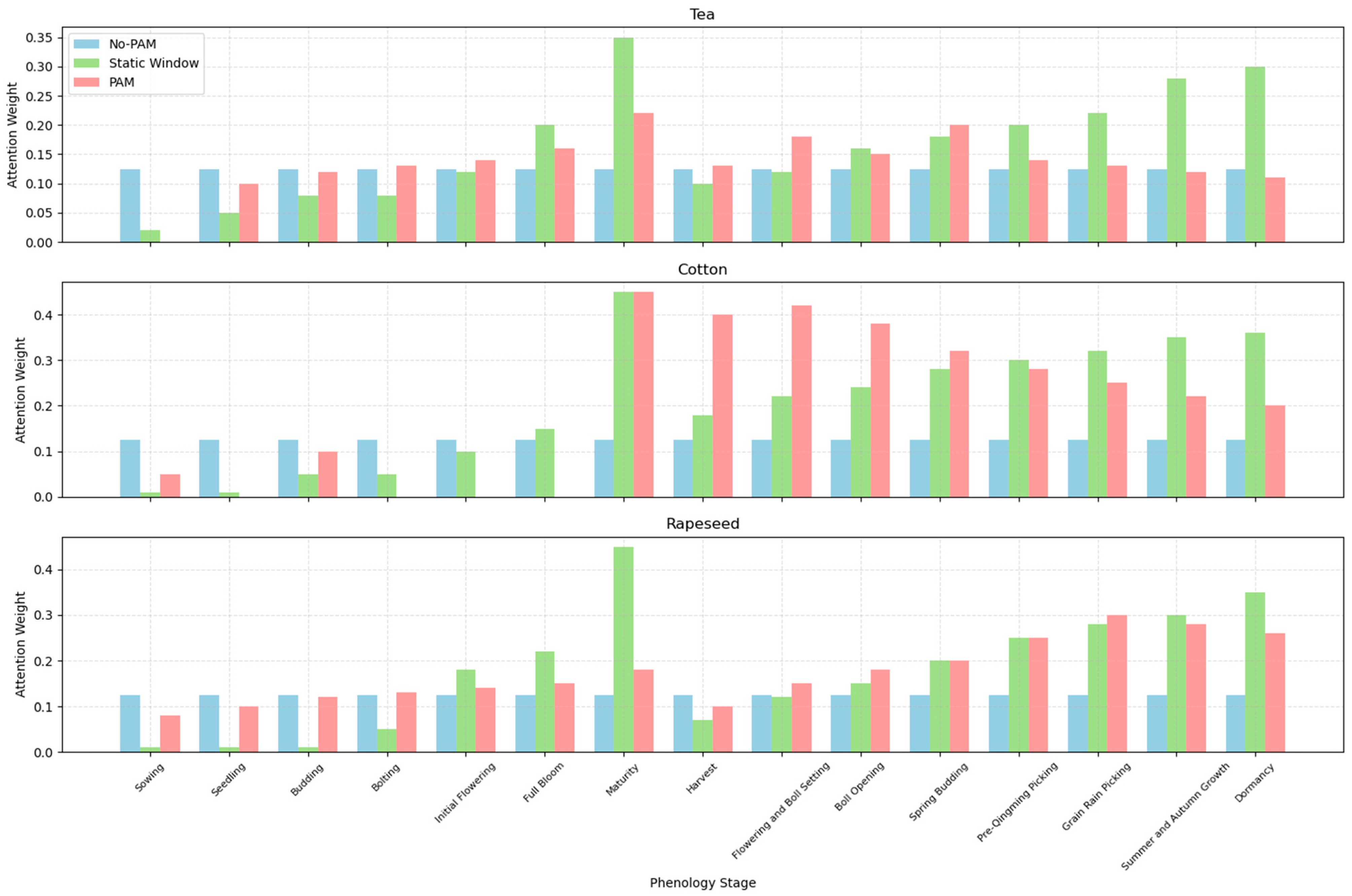
3.3. Phenology-Aware Module (PAM) Module

The PAM module aims to address the rapid changes in spectral characteristics of crops during their growth cycle by dynamically adjusting the model’s attention to different growth stages. Traditional phenological models often rely on static time windows, which overlook the dynamic changes in crop growth stages, making them less flexible when dealing with rapidly changing remote-sensing data. To solve this problem, this study proposes the PAM module, which dynamically allocates different attention weights for each time step to more accurately capture the key features of crops at different phenological stages. The following is a detailed introduction to the PAM module.

3.3.1. Stage Encoding

The first step of the PAM module is to transform the discrete phenological stages (such as sowing, flowering, and harvesting) into feature representations that the model can use. We achieve this by encoding the phenological stages for each time step. Specifically, the phenological stage is first represented as a one-hot encoded vector $P_t\in R^S$, and then mapped to the feature space through a linear transformation (see Formula (7)):

$$P_t^{\prime }=W_p{P}_t+b_p$$

(7)

where $W_p$ is the learnable weight matrix, and $b_p$ is the bias term. This encoding method not only preserves the original meaning of the phenological information but also provides a compatible foundation for subsequent multi-scale perception and feature fusion.

3.3.2. Multi-Scale Phenology Perception

After encoding the phenological information, we need to further extract the changing features at different time scales during the crop growth process. Crop growth dynamics involve patterns at multiple time scales—from short-term fluctuations to mid-term growth stages and long-term seasonal trends. To address this, the PAM module introduces a multi-scale phenology perception mechanism. We use multiple parallel 1D convolution branches with different dilation rates to simultaneously capture short-term, mid-term, and long-term dependencies:

Short-term Convolution (1 × 3 kernel, 64 filters): Focuses on subtle changes between adjacent time steps.

Mid-term Convolution (1 × 5 kernel, 64 filters): Extracts mid-term phenological patterns, such as key transitions during the growing period.

Long-term Convolution (1 × 7 kernel, 64 filters): Captures long-term trends across the entire growth cycle.

After each convolution operation, we apply the ReLU activation function to introduce non-linearity, and then fuse these multi-scale features using a learnable weight coefficient ${\alpha }_i$ (see Formula (8)):

$$P_t^{\mathrm{final}}=\sum _{i=1}^3{\mathsf{\alpha }}_i·{\mathrm{Conv}}_{{\mathrm{scale}}_i}\left(P_t^{\prime }\right)$$

(8)

Through multi-scale phenology perception, the model can adaptively focus on the most relevant features of the crop growth cycle based on the task requirements, laying the groundwork for subsequent spatiotemporal integration.

3.3.3. Time Attention Generation

Building upon ensuring data quality, we aim for the model to dynamically focus on the critical stages of the crop growth cycle. To achieve this, the PAM module introduces a time attention mechanism to generate attention weights. These weights will be applied to each time step’s features through the time attention weight ${\beta }_t$, dynamically adjusting the model’s focus on different time steps. In this step, the phenological stage feature $P_t^{\prime }$ and the fused temporal features $F_{\mathrm{fused}}$ are combined to calculate the attention weight ${\beta }_t$ (see Formula (9)):

$${\beta }_t=\mathit{softmax}\left(W_{\beta }f·\mathit{tan}h\left(W_p{P}_t^{\mathit{final}}+F_t^{\mathit{fused}}\right)\right)$$

(9)

At this stage, we combine the phenological feature $P_t^{\mathrm{final}}$ and the fused feature $F_t^{\mathrm{fused}}$, and through a non-linear transformation and Softmax function normalization, allow the model to adaptively emphasize the time steps most relevant to the task.

3.3.4. Spatiotemporal Integration

Although temporal features are crucial, spatial context should also be utilized, as crops grow in continuous fields and exhibit spatial patterns. After obtaining the multi-scale temporal features for each location and time, PAM integrates spatial information through a 2D convolution layer. In practice, the output of the temporal convolution stage is a sequence of feature maps. Specifically, a 3 × 3 2D convolution kernel (128 filters, stride 1, ‘same’ padding) is used to extract local spatial features (see Formula (10)):

$$F_{\mathit{PAM}-\mathit{spatial}}^t={\mathit{Conv}}_{3\times 3}\left(F_{\mathit{fused}}^t\right)·{\beta }_t$$

(10)

where ${\beta }_t$ is the time attention weight (to be generated in subsequent steps), used to dynamically adjust the contribution of each time step. Through this process, temporal information is effectively integrated with spatial information, thereby enhancing the model’s performance in complex scenarios.

3.3.5. Fusion Quality Check and Stage Feature Weighting

To address the common issues of noise or missing values in remote-sensing data, which can affect the effectiveness of feature fusion, and to enhance the model’s robustness, we introduce a fusion quality check mechanism. Specifically, the time attention weight is adjusted by calculating the variance of the fused feature $F_{\mathrm{fused}}^t$. This ensures that the model reduces its attention on time steps with lower data quality, thereby focusing on more reliable data and providing a more stable foundation for subsequent attention generation (see Formula (11)).

$${\beta }_t^{\prime }={\beta }_t·\left(1-\mathrm{Var}\left(F_t^{\mathrm{fused}}\right)\right)$$

(11)

After obtaining the time attention weights ${\beta }_t$, we perform a weighted sum of the spatiotemporal features to generate the final output of the PAM module (see Formula (12)):

$$F_{\mathrm{PAM}}=\sum {\left(t=1\right)}^{1}2{\beta }_t^{\prime }·F_t^{\mathrm{PAM}-\mathrm{spatial}}$$

(12)

This step integrates the spatiotemporal information of the 12 times steps into a comprehensive feature representation, preserving both temporal dynamics and spatial context, thus providing high-quality input for the subsequent segmentation task.

As shown in Figure 7, specifically, the PAM module achieves dynamic perception of different growth stages by transforming crop phenological information into a continuous feature space and combining it with the temporal features from remote-sensing data. The phenological information of non-food crops is mapped into a continuous vector representation, where each stage’s information is mapped to the feature space using one-hot encoding and linear transformation. These pieces of information are fused with the temporal features of the remote-sensing data and dynamically adjusted through an adaptive attention mechanism to shift the model’s focus. Compared to traditional methods based on fixed time windows, PAM can automatically adjust its focus according to the crop’s growth stage, ensuring efficient utilization of features during the crop’s key growth stages, such as flowering and maturation.

3.4. Decoder

The encoder outputs high-level semantic feature maps, and the resulting deep and shallow semantic features are passed to the decoder [33]. However, since the VIT network is a powerful feature extractor and does not include a corresponding decoder for performing the semantic segmentation task, we use the decoder designed by Xu et al. [34] specifically for Transformers as the decoder for the VIT network. The decoder therefore unfolds as four “bridge” stages that successively upsample the ViT token maps from 1/32 to 1/4 resolution. Each stage first applies a 1 × 1 projection to match channel width, injects local context through a depth-wise 3 × 3 convolution (a lightweight substitute for windowed self-attention), and then blends the result with the lateral encoder feature via a sigmoid-controlled skip-fusion gate. After the final fusion, a SegFormer-style MLP head (depth-wise conv → GELU → 1 × 1 conv) produces the full-resolution logits. Although the average F1 gain over a standard U-Net decoder is only +3.59 percentage points, statistical testing shows the improvement is significant, and the decoder delivers a much larger boost to the minority cotton class while remaining lighter and faster to train than its CNN counterpart. For these reasons we retain this Transformer-adapted decoder in the final network. The core idea of this decoder is to use upsampling to recover spatial resolution, as shown in the following equation (see Formula (13)).

$$X_{\mathrm{upsampled}}=\mathrm{Upsample}\left(X_{\mathrm{encoded}},s\right)$$

(13)

where $X_{\mathrm{encoded}}$ is the low-resolution feature map obtained from the encoder, and s is the upsampling factor. The skip connections combine low-level detail features with high-level semantic features as follows: $X_{\mathrm{skip}}=\mathrm{Concat}\left(X_{\mathrm{encoded}},X_{\mathrm{upsampled}}\right)$, while the Transformer processes global dependencies. Here, $X_{\mathrm{encoded}}$ is the feature map output by the encoder, and $X_{\mathrm{upsampled}}$ is the upsampled feature map. Finally, the classification is performed using the Softmax function, generating pixel-level classification results with the same size as the input image (see Formula (14)).

$$\widehat{y}=\mathit{Softmax}\left(W_{\mathit{output}}{X}_{\mathit{final}}\right)$$

(14)

where $X_{\mathrm{final}}$ is the final output that integrates all of the processed features, and $W_{\mathrm{output}}$ is the learnable weight matrix used for the output.

3.5. Loss Function

Since our study focuses on multi-class semantic segmentation of large-scale non-food crops, and due to the statistical imbalance between the number of target pixels and background pixels in the dataset, there is a class imbalance issue, as shown in

Table 2. Statistical data of non-food crop classes and their proportion of the total image pixels in the dataset.

Object Pixels Ratio
Dataset	HN-NG Set Object Pixels (Proportion)	CCD Set Object Pixels (Proportion)
Training	46,355,337 (8.21%)	5,571,000 (4.78%)
Validation	15,451,779 (2.74%)	1,194,480 (1.02%)
Test	15,451,779 (2.74%)	1,202,040 (1.07%)
Total	77,258,895 (13.69%)	7,967,520 (6.83%)

.

For this study, we chose to use a combination of Weighted Cross-Entropy Loss and Dice Loss [35] to balance classification accuracy and segmentation quality (see Formula (15)).

$$\mathrm{Loss}={\lambda }_1·W\mathrm{CE}+{\lambda }_2·\mathrm{Dice} \mathrm{Loss}$$

(15)

where ${ \lambda }_1$ and ${\lambda }_2$ are the weight coefficients used to balance the two losses.

The “Object Pixels Ratio” refers to the percentage of target pixels relative to the total number of pixels in the entire image. This metric is used to measure the spatial distribution density of the target in the image, with a value range of 0% to 100%.

3.6. Evaluation Metrics

In this study, we used several evaluation metrics to measure the model’s performance in the remote-sensing image segmentation task. Due to the class imbalance and large background regions in remote-sensing images, these metrics provide a comprehensive reflection of the model’s performance in handling large-scale, multi-class semantic segmentation tasks. We used the following main evaluation metrics: accuracy, recall, F1-score, IoU, and mPA. Accuracy represents the proportion of correctly predicted positive instances among all positive predictions. This is a key metric when minimizing false positives is important, as it highlights the model’s ability to avoid misclassifying food areas as non-food areas (see Formula (16)).

$$\begin{gathered} {\displaystyle \frac{\mathrm{Precision}=TP}{\left(TP+FP\right)}} \\ {\displaystyle \frac{\mathrm{Recall}=TP}{\left(TP+FN\right)}} \\ {\displaystyle \frac{F_1\mathrm{score}=\left(2\times \mathrm{Precision}\times \mathrm{Recall}\right)}{\left(\mathrm{Precision}+\mathrm{Recall}\right)}} \end{gathered}$$

(16)

where $TP$ represents the number of pixels correctly predicted as non-food crops, $FN$ represents the number of non-food crop pixels misclassified as background pixels, and $FP$ represents the number of background pixels incorrectly predicted as non-food crops.

Additionally, more comprehensive evaluation metrics include Intersection over Union (IoU) and mean Pixel Accuracy (mPA) mPA is the simple average of per-class pixel accuracies. Because every class contributes equally to the average, mPA highlights performance on minority classes and prevents the majority class from dominating the score, making it a useful complement to IoU and F1 in imbalanced crop-mapping tasks. IoU refers to the proportion of correctly predicted pixels in the union of predicted and actual pixels, while mPA calculates the proportion of correctly classified pixels for each class (see Formula (17)).

$$\begin{gathered} {\displaystyle \frac{\mathrm{IoU}=\mathrm{T}\mathrm{P}}{\left(\mathrm{T}\mathrm{P}+\mathrm{F}\mathrm{P}+\mathrm{F}\mathrm{N}\right)}} \\ \mathit{mPA}={\displaystyle \frac{1}{K+1}}\sum _{t=0}^k{\displaystyle \frac{TP}{TP+FP}} \end{gathered}$$

(17)

The current task involves four classes: rapeseed, tea, cotton, and background. Through the comprehensive analysis of these evaluation metrics, we are able to assess the model’s multi-class semantic segmentation capability in large-scale regional images and complex environments, providing data support for further model optimization and helping us achieve better performance in practical applications.

4. Model Validation and Analysis

In this section, we will validate the superiority of the proposed model for time-series non-food crop classification tasks through detailed descriptions of the dataset, experimental setup, ablation experiments, and comparison experiments. We created a time-series remote-sensing image dataset for non-food crops using remote-sensing data. Given the limited availability of datasets for non-food crop semantic segmentation, we also utilized the Canadian Cropland Dataset (CCD) (https://github.com/bioinfoUQAM/Canadian-cropland-dataset-github, accessed on 6 February 2025), which contains 78,536 high-resolution geo-referenced images for 10 major crop types over 5 months (June to October) and 4 years (2017–2020). Each image includes 12 main spectral bands as well as a series of bands corresponding to vegetation indices (GNDVI, NDVI, NDVI45, OSAVI, and PSRI), covering agricultural croplands in Canada [36]. In the comparison experiments, we compared the classification results of PAM with those from other deep-learning models, evaluated the classification results on both the self-made dataset and the Canadian Cropland Dataset, and also examined the classification results when the decoder in our model was replaced with another type of decoder. In the ablation experiments, we sequentially removed the phenology-aware module based on phenology information and the fusion module based on MTAF from the original model to verify the effectiveness of the entire model.

4.1. Experimental Setup

All models in this experiment were implemented using the PyTorch framework (version 2.0.1). Training and testing were carried out on the high-performance computing platform of China University of Geosciences (Beijing), leveraging NVIDIA A800 GPUs (80 GB) with CUDA 11.8 for acceleration. A weighted combination of Cross-Entropy Loss and Dice Loss was adopted as the loss function and optimized with Adam. The learning rate was dynamically updated on the basis of the F1-score, with the patience parameter set to 15. The initial learning rate was set to 1 × 10⁻⁴. A ReduceLROnPlateau scheduler monitored the validation-set F1-score after each epoch; if no improvement was observed for 15 epochs (patience = 15), the learning rate was multiplied by a factor of 0.5. To stabilize early optimization, a linear warm-up from 0 to the base learning rate was applied over the first five epochs. Training continued until either the maximum epoch count (200) was reached or the learning rate decayed below 1 × 10⁻⁶, whichever came first. These settings were selected empirically to balance convergence speed and generalization. Each input patch was resized to 512 × 512 pixels, the maximum number of training epochs was 200, and the batch size was 20. Details of the experimental dataset are provided in Section 2.3.

4.2. Ablation Experiments

To validate the effectiveness of different parts of the PVM model in the non-food crop classification task, we conducted three sets of ablation experiments. After experiments with the complete model, we performed experiments by removing the PAM module and the MTAF module, respectively. The baseline model is taken as the reference point with the complete PVM model.

(1)

Using the complete PVM model for the experiment, the results were evaluated and used as the testing benchmark for the subsequent modules.

(2)

Testing the effect of the PAM module: We conducted an experiment where the PAM module was removed, and the MTAF + VIT + Decoder were used for the experiment. After obtaining the results, we evaluated the impact on non-food crop pixel segmentation.

(3)

After removing the MTAF module: We fine-tuned the model to adapt to the absence of this module and conducted a complete experiment. The results were analyzed to assess the potential impact of time-series data fusion on segmentation tasks.

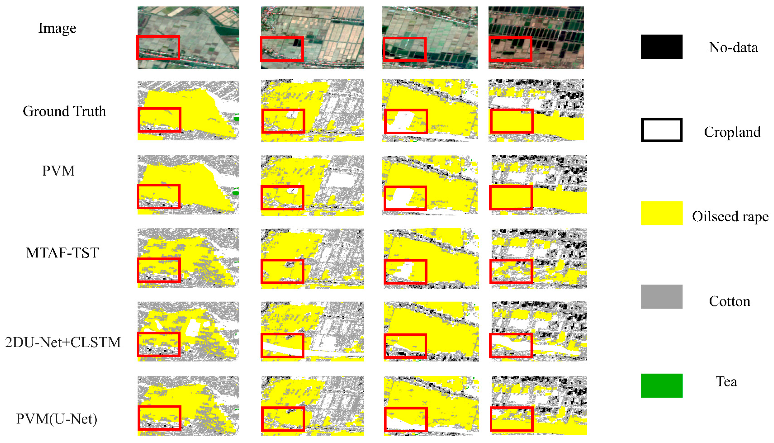
4.3. Comparative Study

In this Section, we compare the experimental results of the PVM model with those from the MTAF-TST model proposed by Yan et al. [31] and the 2DU-Net+CLSTM model studied by R.M. Rustowicz et al. [37], using the non-food crop dataset. The reason for selecting these two models is that they are representative studies in the field of time-series remote-sensing image semantic segmentation and provide comprehensive benchmarks for evaluating the effectiveness and advantages of the proposed method. Additionally, we replaced the decoder in the PVM model with a U-Net decoder to verify the performance of the decoder in our model.

The proposed PVM method was compared with the two aforementioned methods and the widely used semantic segmentation decoder as follows:

(1)

MTAF-TST model: This is a spatiotemporal transformer (MTAF-TST) semantic segmentation framework based on multi-source temporal attention fusion, utilizing optical and SAR time-series data for land cover semantic segmentation. The model uses a Transformer-based spatiotemporal feature extraction module to mine long-range temporal dependencies and high-level spatial semantic information, making it highly suitable for multi-class semantic segmentation of large-area time-series data.

(2)

2DU-Net+CLSTM: This model combines 2D U-Net for image segmentation and CLSTM for time-series processing, used for pixel-level crop type classification from remote-sensing images. By capturing spatial features and temporal dependencies, it provides instantaneous crop state information.

(3)

U-Net Decoder: The U-Net decoder adopts an upsampled (deconvolution) structure with skip connections. It recovers spatial resolution by concatenating feature maps from the encoder with upsampled feature maps from the decoder. It is suitable for multi-class segmentation tasks, making predictions for each pixel for multi-class classification.

Following these three methods, testing was conducted on both the self-made dataset and the Canadian Cropland Dataset. The models were trained and validated independently for each scenario using the same evaluation metrics.

5. Results

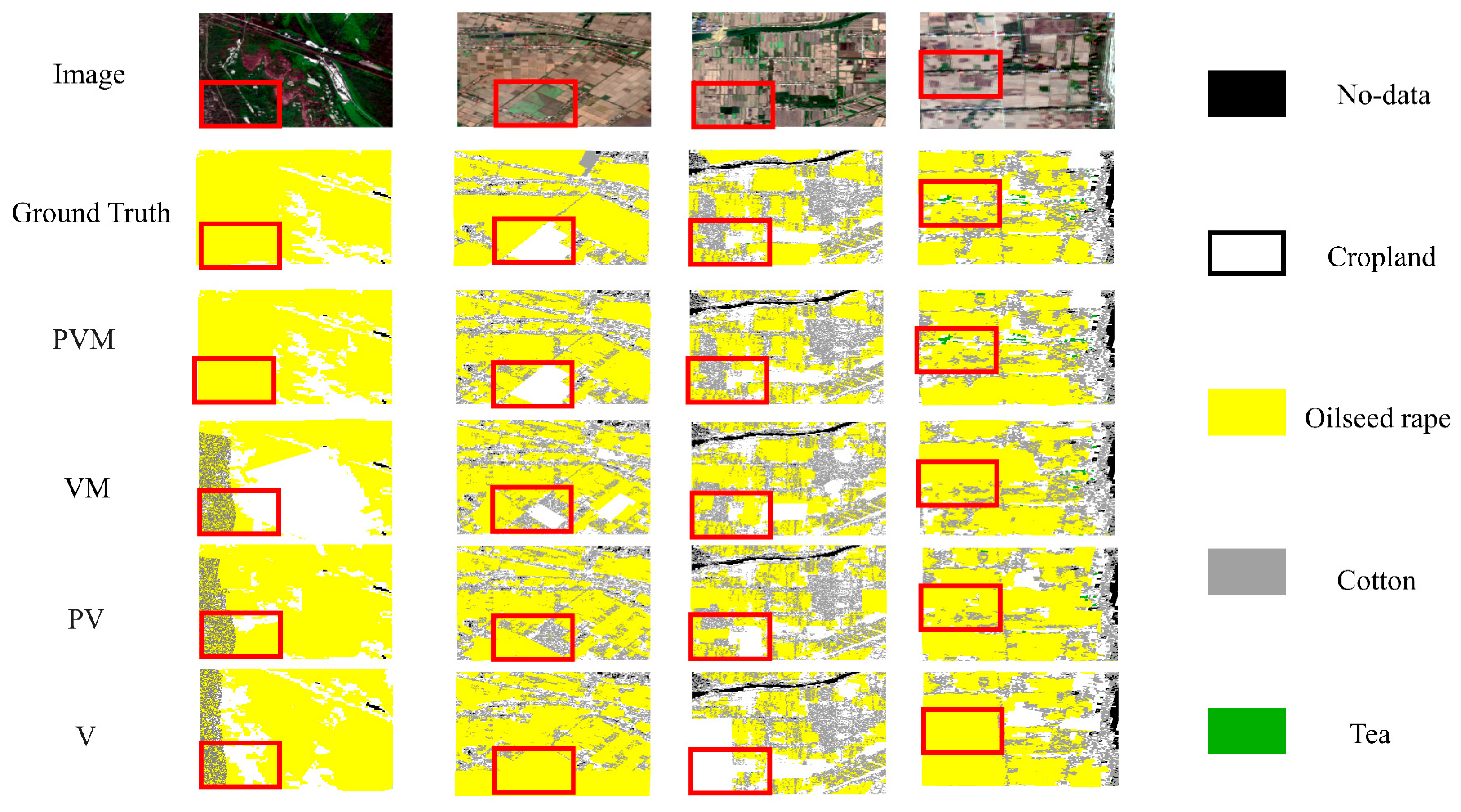
5.1. Ablation Experiment Results

In the ablation experiments, we tested the complete PVM model, the PV model with the PAM module removed, the VM model with the MTAF module removed, and the baseline V model without any modules on the HN-NG Set and CCD Set datasets. Some of the experimental visualization results are shown in Figure 8. As shown in

Table 3. Ablation experiment results of PVM on the HN-NG Set dataset.

Methods	HN-NG Set
	Precision (%)	Recall (%)	F1_Score (%)	IoU (%)	mPA (%)
PVM	82.16	80.04	74.84	61.38	70.46
VM	80.15	76.84	70.19	55.22	67.73
PV	76.47	74.18	66.27	52.52	63.33
V	72.36	65.69	60.71	45.28	58.04

, on the HN-NG Set, the PVM model exhibited high performance across all metrics, with Precision at 82.16%, Recall at 80.04%, F1-score reaching 74.84%, IoU at 61.38%, and mPA at 70.46%. In terms of the impact of adding or removing modules, introducing the PAM module (PV compared to V) resulted in an 8.3% increase in IoU, indicating that the phenology-aware mechanism significantly enhanced the model’s ability to identify key growth stages. Additionally, introducing the MTAF module (VM compared to V) led to a 6.2% increase in F1-score, highlighting the importance of multi-source fusion of optical and radar data for modeling complex temporal features. To further validate the model’s generalization ability, we tested the model on the CCD Set.

As shown in

Table 4. Ablation experiment results of PVM on the CCD dataset.

Methods	CCD Set
	Precision (%)	Recall (%)	F1_Score (%)	IoU (%)	mPA (%)
PVM	79.16	75.65	71.93	55.94	66.14
VM	72.38	70.13	66.99	52.37	61.29
PV	69.71	66.74	62.54	47.95	60.11
V	63.34	60.58	56.82	41.28	54.78

, the overall accuracy on the CCD Set is slightly lower than that on the HN-NG Set. The F1-score of the PVM model is 71.93%, which is approximately 2.91% lower than the former. Nevertheless, the contribution trend of the modules remains consistent. After removing the PAM module (VM model), the IoU drops to 52.37%, which further validates the important role of phenology modeling in enhancing time-series recognition capabilities. After removing the MTAF module (PV model), the Recall significantly decreased by 8.91% (from 75.65% to 66.74%). Furthermore, the baseline model (V) performed the worst on both datasets, with an F1-score of only 56.82%. Both sets of experiments collectively confirm that the PAM and MTAF modules play a critical role in improving the model’s ability to perceive the spatial structure and temporal variation features of non-food crops.

To further validate that the PAM module’s temporal modeling mechanism authentically captures each crop’s key growth stages, we compared the model’s learned attention-weight distributions against the actual phenological periods of rapeseed, cotton, and tea. As shown in Figure 9, the PAM-equipped model demonstrates strong sensitivity to critical phenological windows, with attention peaks closely aligning with the Gantt-chart-style phenology calendar in Figure 3. For instance, rapeseed exhibits heightened attention during the full-bloom and maturity phases (March–June), and cotton shows focused attention during the maturity and harvest stages (July–October). Tea presents a more sustained attention pattern peaking after mid-season, consistent with its prolonged growth and summer development characteristics. It is worth noting that all crops are modeled using a unified set of 15 phenological stages to maintain structural consistency across input sequences. For crop-specific stages that do not occur, the model naturally assigns lower attention weights, reflecting their irrelevance. In contrast, the No-PAM variant displays a nearly uniform distribution of attention values across all 15 stages—including those not relevant to certain crops—typically staying within a narrow low-value range (e.g., 0.06–0.08). This lack of temporal differentiation prevents the model from focusing on phenologically meaningful time points. Similarly, the static-window baseline shows some peaks in predefined periods but suffers from temporal rigidity and limited adaptability to crop-specific dynamics, thereby reducing its generalization capability in multi-crop scenarios.

5.2. Comparison Experiment Results

To verify the overall performance advantages of the proposed PVM model, we conducted a comprehensive comparison with two representative time-series remote-sensing semantic segmentation methods—MTAF-TST and 2DU-Net+CLSTM—along with a classic U-Net decoder structure. The experiments were independently trained and tested on the HN-NG Set dataset, and the classification results for some regions are shown in Figure 10.

Figure 10. Comparison experiment results on the Hunan dataset. From left to right, the four regions are: Original Image, PVM, MTAF-TST, 2DU-Net+CLSTM, and PVM (U-Net). PVM, MTAF-TST, 2D U-Net+CLSTM, and PVM (U-Net) represent the classification results of different models on this dataset. As shown in

Table 5. Comparison results of PVM and mainstream models (HN-NG Set).

Methods	HN-NG Set
	Precision (%)	Recall (%)	F1_Score (%)	IoU (%)	mPA (%)
PVM	82.16	80.04	74.84	61.38	70.46
MTAF-TST	80.25	77.94	72.68	58.44	67.82
2DU-Net+CLSTM	77.83	74.88	69.36	54.79	65.40
PVM (U-Net)	79.66	77.12	71.25	56.87	68.23

, overall, the PVM model outperforms the comparison models in all evaluation metrics. The F1-score reaches 74.84%, and the IoU is 61.38%, which are 2.16% and 2.94% higher than the MTAF-TST model, respectively.

Figure 10. Comparison experiment results on the Hunan dataset. From left to right, the four regions are: Original Image, PVM, MTAF-TST, 2DU-Net+CLSTM, and PVM (U-Net). PVM, MTAF-TST, 2D U-Net+CLSTM, and PVM (U-Net) represent the classification results of different models on this dataset. As shown in Table 5, overall, the PVM model outperforms the comparison models in all evaluation metrics. The F1-score reaches 74.84%, and the IoU is 61.38%, which are 2.16% and 2.94% higher than the MTAF-TST model, respectively.

In contrast, the 2DU-Net+CLSTM model has performance bottlenecks when handling complex phenological backgrounds, with an F1-score of 69.36%, significantly lower than PVM, reflecting its relatively limited ability to model complex spatiotemporal evolution features. Furthermore, to analyze the impact of decoder design on model performance, we replaced the original PVM decoder with a classic U-Net decoder structure for comparison experiments. The results show that although this decoder still maintains good performance (F1-score of 71.25%), there is a 3.59% gap compared to the original decoder, indicating that the decoder module designed in this study, optimized based on the VIT feature structure, is better suited for the deep semantic features extracted by the Transformer.

In contrast, the 2DU-Net+CLSTM model exhibits performance bottlenecks when handling complex phenological backgrounds, with an F1-score of 69.36%, significantly lower than that of PVM. This reflects its relatively limited ability to model complex spatiotemporal evolution features. Furthermore, to analyze the impact of decoder design on model performance, we replaced the original PVM decoder with a classic U-Net decoder structure for comparison experiments. The results show that, although this decoder still maintains good performance (F1-score of 71.25%), there is a 3.59% gap compared to the original decoder, indicating that the decoder module designed in this study, optimized based on the VIT feature structure, is better suited for the deep semantic features extracted by the Transformer.

To further validate the generalization ability of the PVM model, we conducted additional comparison experiments on the CCD Set dataset. As shown in

Table 6. Comparison results of PVM and mainstream models (CCD Set).

Methods	CCD Set
	Precision (%)	Recall (%)	F1_Score (%)	IoU (%)	mPA (%)
PVM	79.16	75.65	71.93	55.94	66.14
MTAF-TST	77.06	75.28	69.14	56.15	65.04
2DU-Net+CLSTM	74.42	70.76	66.55	51.83	62.87
PVM (U-Net)	76.38	74.19	68.24	54.26	64.78

, despite facing more complex climatic conditions and crop distribution differences in this region, PVM still leads in all evaluation metrics, with an F1-score of 71.93% and IoU of 55.94%, which are 2.79% and 0.21% higher than the MTAF-TST model, respectively. In contrast, the performance of the 2DU-Net+CLSTM model in the CCD region declined more significantly, with an F1-score of only 66.55%, indicating that its cyclic structure-based temporal modeling faces bottlenecks under conditions of cloud cover and incomplete time-series data.

To further investigate the source of the model’s performance improvement, we replaced the original PVM decoder with the classic U-Net decoder for a comparative experiment. Although the variant model still performed relatively stably on the CCD Set (F1-score of 68.24%, IoU of 54.26%), the F1-score and IoU dropped by 3.69% and 1.68%, respectively, compared to the complete PVM. This result further confirms that the decoder structure we designed has stronger expressive power in adapting to the deep spatiotemporal features output by the Transformer, especially in cross-regional scenarios, where it more accurately restores complex object boundaries and details.

In the experiments on both the HN-NG and CCD regions, the PVM model consistently demonstrated superior accuracy and stability compared to mainstream methods, validating the effectiveness and robustness of the proposed phenology modeling and multi-source fusion mechanisms in large-scale non-food crop semantic segmentation.

6. Discussion

The non-food crop recognition model proposed in this study achieves high-precision classification and robust cross-region generalization in large-scale cropland scenarios by deeply fusing multi-source temporal remote-sensing data with crop phenology information. In the temporal-fusion component, a Transformer-based encoder leverages self-attention to capture global dependencies throughout the crop growth cycle, overcoming the CNN’s inherent bias toward local features. For instance, the model discriminates the distinct temporal signatures of rapeseed during regreening and maturity, yielding a marked sensitivity to critical phenological stages (F1-score = 74.84%). Concurrently, the MTAF module dynamically weights and integrates Sentinel-1 (SAR) and Sentinel-2 (optical) data, addressing the frequent optical-data gaps in southern China’s rainy season. Specifically, during June–August 2022 in Hunan Province, Sentinel-1 VV polarization compensated for cloud-masked optical pixels, boosting classification IoU by 12.6% in missing-data areas. Moreover, as illustrated in Figure 9, the PAM module not only enhances overall performance but, more importantly, transcends the limitations of fixed temporal windows by dynamically weighting key growth periods. Experimental results show that PAM increases recall by 9.3% during the flowering stage—when spectral distinctions are most pronounced—thereby reducing misclassification due to phenological overlap. In terms of cross-domain adaptability, the model attains an mIoU of 55.94% on the Canadian Cropland Dataset (CCD Set). Although this represents a 5.44% performance drop due to region-specific phenological differences, it still outperforms mainstream approaches (e.g., MTAF-TST at 53.12%), confirming that the phenology-window mechanism substantially promotes consistent feature representation across diverse agro-ecological zones.

6.1. Rapid Changes in Spectral Features and Missing Temporal Data in Non-Food Crop Growth Stages

Non-food crop phenological changes are accompanied by marked physiological and morphological transformations that directly influence their spectral signatures. Throughout development—from emergence to maturity—variations in chlorophyll content, leaf structure, and pigmentation induce pronounced fluctuations in reflectance, particularly in the red-edge and near-infrared bands. For example, during the flowering stage, abrupt changes in chlorophyll concentration lead to a sharp increase in near-infrared reflectance, whereas the senescence processes of maturity produce even more conspicuous spectral shifts [38]. When the temporal resolution of remote-sensing data is insufficient, these rapid spectral dynamics—especially at critical phenological windows, such as anthesis or ripening—may not be captured, thereby degrading the model’s ability to recognize and classify non-food crops accurately [39,40].

Although our spatiotemporal fusion algorithm (e.g., MTAF) partially mitigates the temporal sparsity of Sentinel-2 data caused by cloud and rainfall interruptions by operating directly on the original, non-interpolated time series—thus preserving authentic observation discontinuities—it still risks missing key phenological observations. In periods of prolonged cloud cover, critical Sentinel-2 acquisitions may be entirely unavailable, impairing the model’s capacity to learn precise temporal patterns and semantic distinctions. Empirical studies have demonstrated that such time-series gaps, particularly in optical imagery obstructed by clouds, significantly undermine classification performance for non-food crops [41,42,43]. To address this, recent research has proposed multi-source data supplementation—combining Sentinel-3 with Sentinel-2 observations—to impute missing temporal segments, thereby restoring series completeness and enhancing the model’s fidelity in capturing crop growth dynamics during abrupt phenological transitions, ultimately improving overall accuracy and robustness [44].

6.2. Environmental Heterogeneity and Non-Food Crop Phenology Changes: Challenges and Prospects for Adaptive Models

Phenological changes in non-food crops are influenced by a variety of environmental factors, especially climate, soil, and terrain heterogeneity. This environmental heterogeneity leads to significant phenological dynamic changes in non-food crops across different regions and growth stages. For instance, in areas with large differences in climate and soil conditions, the same non-food crop may have different growth rhythms and time points for key growth stages. In this context, static phenological assumptions often fail to adapt to dynamic changes in the local environment, leading to model uncertainty and errors [45]. Static phenological assumptions typically assume that the changes in non-food crop phenology follow fixed patterns, ignoring the impact of climate fluctuations and soil differences. For example, in some areas, the growth stages of non-food crops may be advanced or delayed, thus affecting the changes in spectral features, making it difficult for the model to accurately recognize the key growth stages of non-food crops [46]. Moreover, crop rotation can also cause temporal signal variations. For example, in rice–rapeseed rotation systems, the growth cycles of the two crops differ, with rapeseed’s flowering and maturation phases typically occurring after rice’s growth cycle, leading to significant spectral feature changes in the time-series data [47]. If the model relies on static phenology windows for classification, these variations in growth cycles and phenological stages will lead to misclassification, especially when there is a significant overlap in spectral features between crops [48,49]. To address these limitations, future research could incorporate adaptive phenological models to overcome the shortcomings of static phenological assumptions. By integrating dynamic information, such as meteorological data, soil moisture, and temperature, the model can adjust the phenology window in real-time, flexibly adapting to the growth patterns of different regions and crops. Through adaptive mechanisms, the model can dynamically adjust phenological parameters based on actual crop growth conditions, improving classification accuracy and adaptability.

6.3. Model Deployment Cost Challenges and Optimization Paths: Applications of Cross-Modal Learning and Lightweight Strategies

The practical application of the PVM model faces high deployment costs, which is particularly evident in real-world applications. The current model relies on large-scale labeled data and high-performance computing resources, such as requiring 9990 labeled samples and powerful computational devices like the NVIDIA A800 GPU for training and optimization. However, this poses significant financial pressure and resource investment for grassroots natural resource departments. Preparing large-scale datasets often requires substantial manual annotation, and purchasing and maintaining high-performance computing resources also requires considerable funding, limiting the application of these models in low-resource areas. In addition to the high costs of hardware and data, differences in crop growth and environmental conditions across regions mean that labeled data from some areas may not be directly applicable to other regions, affecting the model’s accuracy and adaptability. Therefore, the quality and regional adaptability of labeled data are also key issues in model deployment. To address this, future research can explore cross-modal contrastive learning or knowledge distillation techniques to deepen semantic alignment between SAR and optical data, reducing fusion errors for fragmented plots [43]. Introducing lightweight Transformer architectures (such as Mobile-VIT) and self-supervised pretraining strategies can compress model parameters by over 30% and reduce annotation costs by utilizing unlabeled time-series data. Additionally, combining probabilistic soft classification maps and uncertainty modeling techniques can help distinguish fuzzy pixels in “non-food-food” transition areas, providing tiered management guidelines for cultivated land protection policies [31,46].

7. Conclusions

This study presents a semantic segmentation model (PVM) that integrates multi-source remote-sensing time series and crop phenology information to address the challenge of classifying diverse non-food crops across large-scale cultivated areas. By introducing a Phenology-Aware Module (PAM) and a Multi-Task Attention Fusion (MTAF) mechanism, the model effectively captures crop growth dynamics and mitigates optical data gaps caused by cloud interference. Experiments demonstrate that PVM achieves an F1-score of 74.84% and IoU of 61.38% on the Hunan dataset, significantly outperforming baseline and benchmark models. Cross-regional validation on the Canadian Cropland Dataset further confirms generalizability, with an F1-score of 71.93% and IoU of 55.94%. Ablation studies reveal the PAM module improves IoU by 8.3% by dynamically focusing on critical phenological stages, while MTAF enhances Recall by 8.91% through complementary modality fusion. These improvements are consistent with gains over existing methods, such as MTAF-TST and 2DU-Net+CLSTM.

The main contributions of this work are as follows: (1) to our knowledge, this is the first study to deeply integrate phenology calendars into time-series segmentation frameworks specifically for non-food crop mapping, enabling dynamic attention to growth-critical stages; (2) an adaptive fusion strategy of radar and optical time-series data ensures temporal continuity in cloudy southern regions; and (3) a Vision Transformer–based decoder structure tailored for remote sensing effectively enhances global spatiotemporal feature representation, improving F1-score by 3.59% over traditional U-Net designs. Overall, the proposed method provides a high-precision approach for monitoring non-food crop land use conversion, with implications for land resource optimization and food-ecology balance.

References

1. Lin, X.; Fu, H. Spatial-Temporal Evolution and Driving Forces of Cultivated Land Based on the PLUS Model: A Case Study of Haikou City, 1980–2020. Sustainability 2022, 14, 14284. [Google Scholar] [CrossRef]
2. Long, H.; Zhang, Y.; Ma, L.; Tu, S. Land Use Transitions: Progress, Challenges and Prospects. Land 2021, 10, 903. [Google Scholar] [CrossRef]
3. Wang, X.; Song, X.; Wang, Y.; Xu, H.; Ma, Z. Understanding the Distribution Patterns and Underlying Mechanisms of Non-Grain Use of Cultivated Land in Rural China. J. Rural Stud. 2024, 106, 103223. [Google Scholar] [CrossRef]
4. Nduati, E.; Sofue, Y.; Matniyaz, A.; Park, J.G.; Yang, W.; Kondoh, A. Cropland Mapping Using Fusion of Multi-Sensor Data in a Complex Urban/Peri-Urban Area. Remote Sens. 2019, 11, 207. [Google Scholar] [CrossRef]
5. Li, Q.; Wang, C.; Zhang, B.; Lu, L. Object-Based Crop Classification with Landsat-MODIS Enhanced Time-Series Data. Remote Sens. 2015, 7, 16091–16107. [Google Scholar] [CrossRef]
6. Zhang, H.; Yuan, H.; Du, W.; Lyu, X. Crop Identification Based on Multi-Temporal Active and Passive Remote Sensing Images. Int. J. Geo-Inf. 2022, 11, 388. [Google Scholar] [CrossRef]
7. Song, X.-P.; Huang, W.; Hansen, M.C.; Potapov, P. An Evaluation of Landsat, Sentinel-2, Sentinel-1 and MODIS Data for Crop Type Mapping. Sci. Remote Sens. 2021, 3, 100018. [Google Scholar] [CrossRef]
8. Yi, Z.; Jia, L.; Chen, Q. Crop Classification Using Multi-Temporal Sentinel-2 Data in the Shiyang River Basin of China. Remote Sens. 2020, 12, 4052. [Google Scholar] [CrossRef]
9. Huang, X.; Liu, J.; Zhu, W.; Atzberger, C.; Liu, Q. The Optimal Threshold and Vegetation Index Time Series for Retrieving Crop Phenology Based on a Modified Dynamic Threshold Method. Remote Sens. 2019, 11, 2725. [Google Scholar] [CrossRef]
10. Valero, S.; Arnaud, L.; Planells, M.; Ceschia, E. Synergy of Sentinel-1 and Sentinel-2 Imagery for Early Seasonal Agricultural Crop Mapping. Remote Sens. 2021, 13, 4891. [Google Scholar] [CrossRef]
11. Orynbaikyzy, A.; Gessner, U.; Mack, B.; Conrad, C. Crop Type Classification Using Fusion of Sentinel-1 and Sentinel-2 Data: Assessing the Impact of Feature Selection, Optical Data Availability, and Parcel Sizes on the Accuracies. Remote Sens. 2020, 12, 2779. [Google Scholar] [CrossRef]
12. Dobrinić, D.; Gašparović, M.; Medak, D. Sentinel-1 and 2 Time-Series for Vegetation Mapping Using Random Forest Classification: A Case Study of Northern Croatia. Remote Sens. 2021, 13, 2321. [Google Scholar] [CrossRef]
13. Li, Q.; Tian, J.; Tian, Q. Deep Learning Application for Crop Classification via Multi-Temporal Remote Sensing Images. Agriculture 2023, 13, 906. [Google Scholar] [CrossRef]
14. Gadiraju, K.K.; Vatsavai, R.R. Remote Sensing Based Crop Type Classification via Deep Transfer Learning. IEEE J. Sel. Top. Appl. Earth Obs. Remote Sens. 2023, 16, 4699–4712. [Google Scholar] [CrossRef]
15. Feng, F.; Gao, M.; Liu, R.; Yao, S.; Yang, G. A Deep Learning Framework for Crop Mapping with Reconstructed Sentinel-2 Time Series Images. Comput. Electron. Agric. 2023, 213, 108227. [Google Scholar] [CrossRef]
16. Li, H.; Wang, G.; Dong, Z.; Wei, X.; Wu, M.; Song, H.; Amankwah, S.O.Y. Identifying Cotton Fields from Remote Sensing Images Using Multiple Deep Learning Networks. Agronomy 2021, 11, 174. [Google Scholar] [CrossRef]
17. Xu, J.; Zhu, Y.; Zhong, R.; Lin, Z.; Xu, J.; Jiang, H.; Huang, J.; Li, H.; Lin, T. DeepCropMapping: A Multi-Temporal Deep Learning Approach with Improved Spatial Generalizability for Dynamic Corn and Soybean Mapping. Remote Sens. Environ. 2020, 247, 111946. [Google Scholar] [CrossRef]
18. Yu, J.; Zhao, L.; Liu, Y.; Chang, Q.; Wang, N. Automatic Crop Type Mapping Based on Crop-Wise Indicative Features. Int. J. Appl. Earth Obs. Geoinf. 2025, 139, 104554. [Google Scholar] [CrossRef]
19. Qiu, B.; Wu, F.; Hu, X.; Yang, P.; Wu, W.; Chen, J.; Chen, X.; He, L.; Joe, B.; Tubiello, F.N.; et al. A Robust Framework for Mapping Complex Cropping Patterns: The First National-Scale 10 m Map with 10 Crops in China Using Sentinel 1/2 Images. ISPRS J. Photogramm. Remote Sens. 2025, 224, 361–381. [Google Scholar] [CrossRef]
20. Nie, H.; Lin, Y.; Luo, W.; Liu, G. Rice Cropping Sequence Mapping in the Tropical Monsoon Zone via Agronomic Knowledge Graphs Integrating Phenology and Remote Sensing. Ecol. Inform. 2025, 87, 103075. [Google Scholar] [CrossRef]
21. Jiang, J.; Zhang, J.; Wang, X.; Zhang, S.; Kong, D.; Wang, X.; Ali, S.; Ullah, H. Fine Extraction of Multi-Crop Planting Area Based on Deep Learning with Sentinel- 2 Time-Series Data. Env. Sci Pollut Res 2025, 32, 11931–11949. [Google Scholar] [CrossRef]
22. Tian, Q.; Jiang, H.; Zhong, R.; Xiong, X.; Wang, X.; Huang, J.; Du, Z.; Lin, T. PSeqNet: A Crop Phenology Monitoring Model Accounting for Phenological Associations. ISPRS J. Photogramm. Remote Sens. 2025, 225, 257–274. [Google Scholar] [CrossRef]
23. Belgiu, M.; Csillik, O. Sentinel-2 cropland mapping using pixel-based and object-based time-weighted dynamic time warping analysis. Remote Sens. Environ. 2018, 204, 509–523. [Google Scholar] [CrossRef]
24. Available online: www.moa.gov.cn (accessed on 6 July 2025).
25. Jia, D.; Gao, P.; Cheng, C.; Ye, S. Multiple-Feature-Driven Co-Training Method for Crop Mapping Based on Remote Sensing Time Series Imagery. Int. J. Remote Sens. 2020, 41, 8096–8120. [Google Scholar] [CrossRef]
26. Lee, J.S.; Jurkevich, L.; Dewaele, P.; Wambacq, P.; Oosterlinck, A. Speckle Filtering of Synthetic Aperture Radar Images: A Review. Remote Sens. Rev. 1994, 8, 313–340. [Google Scholar] [CrossRef]
27. Huang, S.; Liu, D.; Gao, G.; Guo, X. A Novel Method for Speckle Noise Reduction and Ship Target Detection in SAR Images. Pattern Recognit. 2009, 42, 1533–1542. [Google Scholar] [CrossRef]
28. Li, X.; Zhu, W.; Xie, Z.; Zhan, P.; Huang, X.; Sun, L.; Duan, Z. Assessing the Effects of Time Interpolation of NDVI Composites on Phenology Trend Estimation. Remote Sens. 2021, 13, 5018. [Google Scholar] [CrossRef]
29. Cai, Z.; Jönsson, P.; Jin, H.; Eklundh, L. Performance of Smoothing Methods for Reconstructing NDVI Time-Series and Estimating Vegetation Phenology from MODIS Data. Remote Sens. 2017, 9, 1271. [Google Scholar] [CrossRef]
30. Yang, J.; Huang, X. 30 m Annual Land Cover and Its Dynamics in China from 1990 to 2019. Earth Syst. Sci. Data Discuss. 2021, 13, 3907–3925. [Google Scholar] [CrossRef]
31. Yan, J.; Liu, J.; Liang, D.; Wang, Y.; Li, J.; Wang, L. Semantic Segmentation of Land Cover in Urban Areas by Fusing Multisource Satellite Image Time Series. IEEE Trans. Geosci. Remote Sens. 2023, 61, 4410315. [Google Scholar] [CrossRef]
32. Dosovitskiy, A.; Beyer, L.; Kolesnikov, A.; Weissenborn, D.; Zhai, X.; Unterthiner, T.; Dehghani, M.; Minderer, M.; Heigold, G.; Gelly, S.; et al. An Image Is Worth 16x16 Words: Transformers for Image Recognition at Scale. arXiv 2020, arXiv:2010.11929. [Google Scholar]
33. Zhou, S.; Nie, D.; Adeli, E.; Yin, J.; Lian, J.; Shen, D. High-Resolution Encoder–Decoder Networks for Low-Contrast Medical Image Segmentation. IEEE Trans. Image Process. 2019, 29, 461–475. [Google Scholar] [CrossRef]
34. Xu, Z.; Zhang, W.; Zhang, T.; Yang, Z.; Li, J. Efficient Transformer for Remote Sensing Image Segmentation. Remote Sens. 2021, 13, 3585. [Google Scholar] [CrossRef]
35. Jadon, S. A Survey of Loss Functions for Semantic Segmentation. In Proceedings of the 2020 IEEE Conference on Computational Intelligence in Bioinformatics and Computational Biology (CIBCB), Via del Mar, Chile, 27–29 October 2020; pp. 1–7. [Google Scholar]
36. Jacques, A.A.B.; Diallo, A.B.; Lord, E. The Canadian Cropland Dataset: A New Land Cover Dataset for Multitemporal Deep Learning Classification in Agriculture. arXiv 2023, arXiv:2306.00114. [Google Scholar]
37. M Rustowicz, R.; Cheong, R.; Wang, L.; Ermon, S.; Burke, M.; Lobell, D. Semantic Segmentation of Crop Type in Africa: A Novel Dataset and Analysis of Deep Learning Methods. In Proceedings of the IEEE/CVF Conference on Computer Vision and Pattern Recognition Workshops, Long Beach, CA, USA, 16–17 June 2019; pp. 75–82. [Google Scholar]
38. Gao, F.; Zhang, X. Mapping Crop Phenology in Near Real-Time Using Satellite Remote Sensing: Challenges and Opportunities. J. Remote Sens. 2021, 2021, 8379391. [Google Scholar] [CrossRef]
39. Kasampalis, D.A.; Alexandridis, T.K.; Deva, C.; Challinor, A.; Moshou, D.; Zalidis, G. Contribution of Remote Sensing on Crop Models: A Review. J. Imaging 2018, 4, 52. [Google Scholar] [CrossRef]
40. Zhao, Y.; Potgieter, A.B.; Zhang, M.; Wu, B.; Hammer, G.L. Predicting Wheat Yield at the Field Scale by Combining High-Resolution Sentinel-2 Satellite Imagery and Crop Modelling. Remote Sens. 2020, 12, 1024. [Google Scholar] [CrossRef]
41. Roßberg, T.; Schmitt, M. Dense NDVI Time Series by Fusion of Optical and SAR-Derived Data. IEEE J. Sel. Top. Appl. Earth Obs. Remote Sens. 2024, 17, 7748–7758. [Google Scholar] [CrossRef]
42. Belgiu, M.; Stein, A. Spatiotemporal Image Fusion in Remote Sensing. Remote Sens. 2019, 11, 818. [Google Scholar] [CrossRef]
43. Bai, B.; Tan, Y.; Donchyts, G.; Haag, A.; Weerts, A. A Simple Spatio–Temporal Data Fusion Method Based on Linear Regression Coefficient Compensation. Remote Sens. 2020, 12, 3900. [Google Scholar] [CrossRef]
44. Bellvert, J.; Jofre-Ĉekalović, C.; Pelechá, A.; Mata, M.; Nieto, H. Feasibility of Using the Two-Source Energy Balance Model (TSEB) with Sentinel-2 and Sentinel-3 Images to Analyze the Spatio-Temporal Variability of Vine Water Status in a Vineyard. Remote Sens. 2020, 12, 2299. [Google Scholar] [CrossRef]
45. Bregaglio, S.; Ginaldi, F.; Raparelli, E.; Fila, G.; Bajocco, S. Improving Crop Yield Prediction Accuracy by Embedding Phenological Heterogeneity into Model Parameter Sets. Agric. Syst. 2023, 209, 103666. [Google Scholar] [CrossRef]
46. Ceglar, A.; van der Wijngaart, R.; de Wit, A.; Lecerf, R.; Boogaard, H.; Seguini, L.; van den Berg, M.; Toreti, A.; Zampieri, M.; Fumagalli, D.; et al. Improving WOFOST Model to Simulate Winter Wheat Phenology in Europe: Evaluation and Effects on Yield. Agric. Syst. 2019, 168, 168–180. [Google Scholar] [CrossRef]
47. Arias, M.; Campo-Bescós, M.Á.; Álvarez-Mozos, J. Crop Classification Based on Temporal Signatures of Sentinel-1 Observations over Navarre Province, Spain. Remote Sens. 2020, 12, 278. [Google Scholar] [CrossRef]
48. Chen, Y.; Hu, J.; Cai, Z.; Yang, J.; Zhou, W.; Hu, Q.; Wang, C.; You, L.; Xu, B. A Phenology-Based Vegetation Index for Improving Ratoon Rice Mapping Using Harmonized Landsat and Sentinel-2 Data. J. Integr. Agric. 2024, 23, 1164–1178. [Google Scholar] [CrossRef]
49. Liu, J.; Zhu, W.; Atzberger, C.; Zhao, A.; Pan, Y.; Huang, X. A Phenology-Based Method to Map Cropping Patterns under a Wheat-Maize Rotation Using Remotely Sensed Time-Series Data. Remote Sens. 2018, 10, 1203. [Google Scholar] [CrossRef]
Figure 1. (a) Geographical location of Hunan Province, China. (b) Land use type map of Hunan Province.
Remotesensing 17 02346 g001
Figure 2. (a) Sentinel-2 time-series data for some regions after data processing. (b) Sentinel-1 time-series data for some regions. (c) Sentinel-2 image count. (d) Sentinel-1 image count.
Remotesensing 17 02346 g002
Figure 3. Phenology calendar of major non-food crops in Hunan Province.
Remotesensing 17 02346 g003
Figure 4. Illustrates the overall architecture of the PAM-MTAF-VIT model.
Remotesensing 17 02346 g004
Figure 5. Principle of the VIT technology, where * stands for positional encoding.
Remotesensing 17 02346 g005
Figure 6. Principle of the MTAF (Multi-Task Attention Fusion) module technology.
Remotesensing 17 02346 g006
Figure 7. Principle diagram of the PAM.
Remotesensing 17 02346 g007
Figure 8. Ablation experiment results on the Hunan dataset. From left to right, the four regions are: Original Image, VM, PV and V. Among them, VM, PM, and V refer to removing the PAM module, VIT module, and PAM and MTAF modules, respectively, in order to verify the validity of each module. This study primarily focuses on identifying farmland plots. Although the figure includes tea garden pixels, due to geographical constraints, tea trees are primarily cultivated in hilly regions, resulting in a very small number of tea garden pixels in the figure that are nearly invisible.
Remotesensing 17 02346 g008
Figure 9. Distribution of attention weights across phenological stages for three non-food crops under different model variants (PAM, No-PAM, Static-Window). The rows correspond to canola, cotton, and tea, respectively. The columns represent the full model (with PAM), the No-PAM variant with temporal attention removed, and the Static-Window baseline with fixed temporal windows. The PAM curves exhibit sharp peaks during key phenological stages—Stage8–Stage9 (flowering stage) for canola, Stage11–Stage12 (boll stage) for cotton, and Stage7–Stage8/Stage10 (spring and summer flush) for tea—whereas both baselines show only broad or misaligned peaks. The gray shaded areas indicate the stages with the largest recall improvement (see Table 3), visually demonstrating that temporal attention enables the model to focus on the most discriminative phenological windows.
Remotesensing 17 02346 g009