Abstract
Underwater acoustic target recognition (UATR) is challenged by complex marine noise, scarce labeled data, and inadequate multi-scale feature extraction in conventional methods. This study proposes DART-MT, a semi-supervised framework that integrates a Dual Attention Parallel Residual Network Transformer with a mean teacher paradigm, enhanced by domain-specific prior knowledge. The architecture employs a Convolutional Block Attention Module (CBAM) for localized feature refinement, a lightweight New Transformer Encoder for global context modeling, and a novel TriFusion Block to synergize spectral–temporal–spatial features through parallel multi-branch fusion, addressing the limitations of single-modality extraction. Leveraging the mean teacher framework, DART-MT optimizes consistency regularization to exploit unlabeled data, effectively mitigating class imbalance and annotation scarcity. Evaluations on the DeepShip and ShipsEar datasets demonstrate state-of-the-art accuracy: with 10% labeled data, DART-MT achieves 96.20% (DeepShip) and 94.86% (ShipsEar), surpassing baseline models by 7.2–9.8% in low-data regimes, while reaching 98.80% (DeepShip) and 98.85% (ShipsEar) with 90% labeled data. Under varying noise conditions (−20 dB to 20 dB), the model maintained a robust performance (F1-score: 92.4–97.1%) with 40% lower variance than its competitors, and ablation studies validated each module’s contribution (TriFusion Block alone improved accuracy by 6.9%). This research advances UATR by (1) resolving multi-scale feature fusion bottlenecks, (2) demonstrating the efficacy of semi-supervised learning in marine acoustics, and (3) providing an open-source implementation for reproducibility. In future work, we will extend cross-domain adaptation to diverse oceanic environments.
1. Introduction
Underwater acoustic target recognition (UATR) has emerged as a critical enabling technology for maritime situational awareness, with applications in naval defense, marine ecosystem monitoring, and underwater cultural heritage preservation [1]. The increasing complexity of underwater operations necessitates robust recognition systems capable of distinguishing diverse acoustic signatures in dynamic oceanic environments characterized by multipath propagation, ambient noise interference, and target mobility [2]. Despite significant progress in supervised learning paradigms, this field faces persistent challenges in achieving reliable performance under data-scarce conditions that are inherent to underwater scenarios.
Traditional UATR methodologies primarily employ handcrafted feature extraction pipelines grounded in signal physics or bio-inspired auditory modeling. Physics-based approaches analyze time-domain attributes (e.g., zero-crossing rate) [3], frequency-domain representations through cepstral analysis [4], and joint time-frequency features via wavelet transforms [5,6,7]. Complementarily, brain-computing-inspired techniques leverage Mel-Frequency Cepstral Coefficients (MFCC) [8] and gamma-tone filtering [9] to simulate human auditory processing. These conventional frameworks, while effective in controlled environments, exhibit three fundamental limitations: (1) overreliance on domain-specific priors [10], (2) inadequate representation of multiscale acoustic patterns [11], and (3) poor generalization to unseen operating conditions [12]. The hybrid feature approaches proposed in recent studies [13,14,15,16,17,18] attempt to mitigate these issues but still produce suboptimal feature fusion owing to their two-dimensional processing architecture.
The advent of deep learning has transformed UATR by enabling hierarchical feature learning, which captures complex signal characteristics [19,20,21,22,23,24,25,26,27,28]. However, this paradigm shift introduces new challenges: (1) the scarcity of publicly available, high-quality annotated datasets, and (2) the computational inefficiency of conventional feature fusion strategies. Existing repositories, such as DeepShip and ShipsEar, suffer from critical limitations: the former lacks realistic background noise diversity, whereas the latter contains insufficient sample volumes for reliable deep model training. As illustrated in Figure 1, the data annotation process in underwater environments involves complex sonar signal interpretation, which further exacerbates the challenges of dataset development.
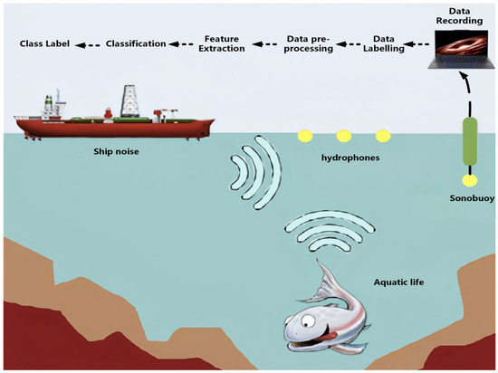
Figure 1.
The flowchart of generating labels with sonar-extracted information.
To address these interrelated issues, this study proposes a Dual Attention Parallel Residual Network Transformer (DART) framework integrated within a mean teacher semi-supervised architecture (DART-MT). The key innovations include (1) the TriFusion Block, a hierarchical feature processor that simultaneously analyzes raw, differential, and cumulative acoustic signals through complementary spectral decomposition techniques (MFCC for spectral envelope, CQT for time-frequency resolution, and FBank for energy dynamics), and (2) a synergistic combination of dual attention mechanisms with residual Transformer modules to enhance feature discriminability. This architecture systematically overcomes two critical barriers in current UATR systems: limited feature representation capacity and data annotation constraints.
The primary contributions of this study are as follows:
- A novel semi-supervised framework (DART-MT) that integrates physics-guided residual networks with dual attention transformers, specifically designed to optimize UATR performance under minimal labeling conditions;
- The TriFusion Block architecture processes complementary signal domains in parallel to establish a 3D feature tensor representation (3 × 128 × 216), which enhances the multi-scale acoustic pattern disentanglement;
- Comprehensive benchmarking across varying data-scarcity scenarios on two public UATR datasets, demonstrating statistically significant performance improvements (p < 0.01) over state-of-the-art methods;
- Theoretical analysis of differential feature processing mechanisms in underwater acoustic signal modeling, with empirical validation of zero-shot learning capabilities.
2. Related Work
This section introduces the background and related work on DART and DART-MT models in the field of underwater acoustic target recognition (UATR).
2.1. Supervised Learning Approaches
Deep learning includes paradigms such as supervised learning, which is commonly used in UATR research. It involves signal analysis and processing to derive features from the labeled samples for classifier construction. Ren et al. [29] created a learnable front-end for UATR systems. Doan et al. [30] used raw time-domain waveforms for a UATR model in low signal-to-noise ratio environments. Khishe [31] integrated wavelet networks with autoencoders using the ShipsEar [32] dataset. Feng et al. [33] applied the Transformer network to UATR, achieving better results than some CNN on the DeepShip [34] dataset. However, these models depend on comprehensive datasets, and the lack of annotated samples hinders the use of a supervised learning framework. In real UATR scenarios, the data are mostly unlabeled and imbalanced, causing challenges for model training and potentially leading to insufficient learning or overfitting issues. This limits the improvement in recognition performance, suggesting that supervised deep learning methods for UATR may be approaching their limits [35,36,37,38,39].
2.2. Unsupervised and Few-Shot Learning
Unsupervised learning methods are crucial for underwater acoustic target recognition because they learn visual representations from unlabeled data. Momentum Contrast (MoCo), introduced by He et al. [40], is one such method that learns features through contrastive learning. However, these methods often face issues such as poor stability and low accuracy in complex underwater environments. Few-shot learning approaches [41,42], which aim to learn from a small number of samples, have shown promise in this field. For instance, Ghavidel et al. [43] explored few-shot learning for sonar data classification. However, the scarcity of diverse underwater samples poses a significant challenge, making it difficult to collect extensive base class data.
In the context of underwater acoustic target recognition, the limited availability of labeled data and the complexity of the underwater environment make it difficult to apply traditional supervised learning methods. Unsupervised and few-shot learning approaches offer potential solutions; however, they need to address the issues of stability and accuracy to be more effective in real-world applications. Recent research has focused on combining these approaches with other techniques, such as semi-supervised learning, to improve the performance of underwater-acoustic target recognition models.
2.3. Semi-Supervised Learning
Semi-supervised learning bridges the gap between supervised and unsupervised techniques. It uses a small set of labeled data and a larger pool of unlabeled data. Algorithms such as FixMatch [44] and contrastive learning frameworks [45] have advanced this field by generating pseudo-labels and enhancing learning performance with limited labeled data.
However, these methods may struggle with data imbalances and zero-shot learning scenarios. The proposed DART-MT model aims to address these issues by integrating a semisupervised learning framework. Advanced network architectures, such as residual networks [46] and fusion networks [47,48] have shown exceptional performance in UATR owing to their adaptability. Attention mechanisms [49,50] are crucial for feature extraction, particularly in noisy environments.
The DART model leverages these techniques by integrating ResNeXt18 for localized feature extraction, CBAM for refined feature enhancement, and a New Transformer Encoder for comprehensive global context understanding. The dual-attention parallel residual network transformer (DART) model is a key component of this approach. The DART-MT variant uses the mean teacher mechanism and pre-trained weights to effectively address sample scarcity in imbalanced datasets. In summary, the DART and DART-MT models build upon advancements in deep learning architectures and semi-supervised learning to address the challenges of UATR, offering a more robust and effective solution for underwater acoustic target recognition.
3. Methodology
Underwater acoustic targets exhibit significant inter-class variations in their acoustic signatures owing to distinct physical generation mechanisms, leading to three primary technical challenges: (1) class imbalance issues in practical monitoring scenarios, (2) model overfitting risks caused by limited training samples, and (3) suboptimal classification performance in zero-shot learning scenarios. To address these challenges and enhance the cross-domain generalization capacity of the DART-MT architecture, we propose a Dual-Attention Representation Transfer (DART) framework specifically designed to enhance cross-domain generalization capabilities through a multi-task learning architecture. This novel mechanism achieves robust feature alignment across heterogeneous domains while maintaining task-specific discriminability using adaptive spectral attention and temporal correlation modules.
3.1. DART-MT
As illustrated in Figure 2, the Dual Attention Parallel Residual Network Transformer (DART-MT) model represents a significant advancement in underwater acoustic target recognition (UATR). It integrates the DART model with a mean teacher semi-supervised learning framework.
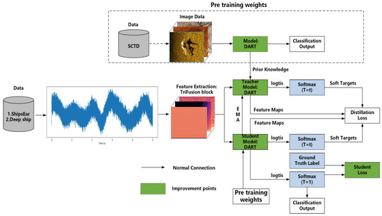
Figure 2.
The overview of the DART-MT model.
The operational workflow is initiated with the TriFusion Block, which processes underwater sonar signals by simultaneously analyzing the raw signal, its temporal derivatives (differential signal), and cumulative features. This parallel processing mechanism transforms sonar signals into a comprehensive multimodal representation, effectively capturing both the static spectral characteristics and dynamic temporal variations inherent in underwater acoustic signatures. At the core of this process, the DART model utilizes a pre-trained teacher model, which incorporates essential prior knowledge for recognizing underwater acoustic targets, to train on the SCTD [51] dataset.
The DART-MT model adopts a semi-supervised learning framework. In this framework, a limited subset of data serves as the input for both the student and teacher models, enabling the generation of soft targets and the inference of classification results. The student model then assimilates prior knowledge from the teacher model through distillation loss and cross-entropy error calculations, optimizing its performance for underwater acoustic target classification tasks.
3.2. DART Model
As illustrated in Figure 3, the Dual Attention Parallel Residual Network Transformer (DART) model represents a significant breakthrough in underwater acoustic target recognition (UATR). By seamlessly integrating state-of-the-art techniques, it optimizes feature extraction and classification accuracy, serving as the core component of the DART-MT.
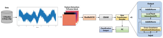
Figure 3.
DART model structure.
The DART model operational process commences with the TriFusion Block, which transforms underwater sonar signals into a feature map. Subsequently, the ResNeXt18 architecture processes the feature map. ResNeXt18, which is renowned for its efficiency in extracting localized image characteristics, acts as a fundamental feature extractor. Leveraging grouped convolution enhances feature richness and facilitates effective hierarchical representation. Through this process, ResNeXt18 extracts and refines high-level features, which are then fed into the Convolutional Block Attention Module (CBAM).
The CBAM plays a pivotal role in refining and enhancing the features output by the ResNeXt18 network. It adaptively modifies the weights of the individual channels and spatial locations. By emphasizing the essential features for classification and suppressing irrelevant data, the CBAM improves the model’s focus. Comprising two core components, channel attention and spatial attention, the CBAM mechanism functions as follows: channel attention assesses the significance of each feature channel, whereas spatial attention pinpoints critical regions within the feature map. This dual-focus approach streamlines feature extraction and strengthens the model’s data representation ability. Integrating the CBAM with ResNeXt18 enables the model to better capture important information from the input data, resulting in more accurate classifications. Additionally, the CBAM mitigates the influence of irrelevant information, allowing the model to concentrate more effectively on relevant data.
The final constituent of the DART model is the New Transformer Encoder. Utilizing its multi-head self-attention mechanism, the New Transformer Encoder captures and integrates global information. This mechanism excels at understanding global contexts and semantic interpretations, thereby significantly enhancing the model’s interpretability and recognition accuracy. By combining ResNeXt18 for localized feature extraction with the New Transformer Encoder for global sequence modeling, the DART model leverages the advantages of both approaches. The incorporation of the CBAM further refines this process, enabling the model to focus on crucial features, capture vital details, and minimize the impact of noise. This synergistic combination substantially improves the model efficiency and accuracy in image classification tasks, presenting a robust and comprehensive solution that capitalizes on the strengths of both Convolutional Neural Networks (CNN) and Transformer architectures.
In conclusion, the DART model stands out because of its integration of ResNeXt18 for localized feature extraction, CBAM for refined feature enhancement, and the New Transformer Encoder for comprehensive global context understanding. This holistic design sets a new standard for UATR, showcasing exceptional capabilities in enhancing performance and recognition accuracy for underwater target classification tasks.
3.2.1. ResNeXt18
The proposed model integrates ResNeXt18, CBAM Attention Mechanism, and Transformer Encoder for recognition classification tasks. ResNeXt18 (the structures are shown in Table 1) functions as a foundational feature extractor, using grouped convolution to enhance feature richness and promote an effective hierarchical representation. The integration of ResNeXt18 allows for the extraction and refinement of high-level features, which are then input into the CBAM. The CBAM optimizes these features by focusing on crucial spatial locations and channels, thereby enhancing the image classification accuracy of the model. Following the CBAM, these optimized features were processed by the Transformer Encoder, which aided in efficient feature transformation and categorization. Overall, ResNeXt18 serves as a critical component, boosting the performance of the model by providing refined input features to subsequent mechanisms, thereby enhancing the overall efficiency and accuracy of classification tasks.

Table 1.
ResNeXt18 structure.
3.2.2. CBAM Attention Mechanism
In the DART model, the Channel-wise Attention Mechanism (CBAM), as shown in Figure 4, is key to refining and enhancing the features from the ResNeXt18 network. The CBAM adaptively adjusts the weights of individual channels and spatial locations, focusing on the essential features for classification and discarding irrelevant data. Integrating the CBAM with ResNeXt18 improved the model’s ability to capture important information from images, leading to more precise classifications. Furthermore, the CBAM reduces the impact of irrelevant information, allowing the model to focus more effectively on pertinent data. The synergy between the CBAM and the Transformer Encoder further enhances the efficacy of the model. While the Transformer Encoder effectively processes input sequences, the CBAM refines the input features, supporting better performance in recognition and classification tasks.
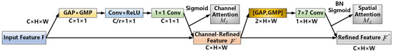
Figure 4.
Structural diagram of CBAM attention mechanism.
The CBAM consists of two core components: channel and spatial attention. Channel attention evaluates the importance of each feature channel, and spatial attention identifies the critical regions in the image. This dual focus streamlines feature extraction and enhances the model’s ability to represent data.
The CBAM attention mechanism is divided into channel and spatial attention; thus, it can be described by the following equation:
The feature map is denoted as . The channel attention feature map is , and the spatial attention feature map is . The symbol represents element-wise multiplication. Meanwhile, and represent the mean pooling and maximum pooling features, respectively. The parameters of the Multi-Layer Perceptron (MLP) are denoted as and . The sigmoid operation is represented by , and the size of the convolution kernel is indicated by .
The Convolutional Block Attention Module (CBAM) utilizes a convolution with kernel size . This convolution operation captures long-range spatial dependencies within the input feature maps. By analyzing the relationships among features that are dispersed across the input data, the CBAM can grasp the global context and understand the overall structure of the input. The relatively large convolution kernel size enables CBAM to better capture complex patterns and spatial relationships. Consequently, it achieves more effective feature optimization, ultimately enhancing the accuracy of tasks such as image classification.
The CBAM enhances feature extraction by applying channel and spatial attention mechanisms sequentially, ensuring that the model focuses on important image areas. Consequently, the CBAM is a key element in optimizing the model performance by supplying the Transformer Encoder with high-quality input features.
3.2.3. New Transformer Encoder
In the field of underwater sonar target recognition, the complex and variable underwater noise environment has always been a key factor restricting the performance of traditional Transformer Encoders. Owing to the high sensitivity of traditional Transformer Encoders to noise, when processing underwater sonar signals, they are extremely prone to the problem of target feature blurring, which in turn leads to a significant decline in model recognition accuracy. To tackle this technical bottleneck, this study proposes a novel Transformer Encoder architecture that achieves significant performance improvement by integrating two core sub-modules: XCAttention and LPI. Figure 3 demonstrates the critical role of the proposed Transformer Encoder.
As the core innovation of the novel Transformer Encoder, the XCAttention sub-module represents a revolutionary improvement over the traditional self-attention mechanism. When the traditional self-attention mechanism processes underwater sonar signals, severe noise interference makes it difficult to accurately locate and focus on the key information, resulting in low feature extraction efficiency. In contrast, the XCAttention submodule introduces a cross-covariance mechanism, enabling it to measure the correlation between features at different positions during the attention calculation process. This mechanism can be expressed as
where and are the normalized query and key vectors, and is a learnable temperature parameter. This mechanism enables XCAttention to efficiently extract the key information required for target recognition from complex underwater sonar signals. When processing sonar signals containing multiple targets, XCAttention clearly distinguishes the features of different targets through cross-covariance calculations, effectively avoiding feature confusion.
The other core component, the local patch interaction (LPI) module, promotes local patch interaction through depthwise separable convolutions. It first rearranges the input into a format suitable for convolution processing, performs two grouped convolutions with activation function operations, and then reconstructs the output into the original sequence structure. This approach captures fine-grained details and distinguishes valid information from complex signals, particularly suppressing high-frequency noise while preserving low-frequency target features.
In the novel Transformer Encoder, XCAttention and LPI form a powerful synergy through a collaborative framework of “global guidance combined with local refinement,” and their integration process can be expressed as
In the novel Transformer Encoder, the two modules, XCAttention and LPI, work closely together, generating a powerful synergistic effect that greatly improves the model’s performance in underwater sonar feature extraction and processing tasks. Together, they address challenges such as marine environmental noise and the mixing of underwater acoustic target feature information, significantly increasing the model recognition accuracy and overall performance.
3.3. Mean Teacher Semi-Supervised Learning
The proposed methodology begins with feature extraction from underwater acoustic signals, which are often characterized by small sample sizes. The numerical processing module extracts audio signal frames and converts them into a TriFusion Block, effectively capturing the original signal and its temporal dynamics. As shown in Figure 2, the DART model, which constructs the network model and its parameters, was used to train the SCTD data. The teacher model, equipped with pre-trained weights, contains essential prior knowledge for recognizing underwater acoustic targets.
Next, a small subset of data from other datasets is input into both the student and pre-trained teacher models, which then generates soft targets and infers the classification results. The soft targets were calculated using the softmax function, as expressed in Equation (7).
where logits for the class, is weight that regulates the significance of individual soft targets. This article is set to .
The student model assimilates prior knowledge from the teacher model, including response and feature information. Distillation loss, which comprises response and feature losses, quantifies the similarity between the student and teacher models. Specifically, response-based loss and feature-based loss are computed using KL divergence, quantifying the degree of similarity between the probability distributions of soft targets and feature maps, as detailed in Equations (8) and (9).
In this context, serves as a soft target for the student model output pertaining to sample , while represents the corresponding soft target for the teacher model output on the same sample. Similarly, denotes the feature maps generated by the final hidden layer of the student model when processing sample , whereas corresponds to the feature maps produced by the teacher model last hidden layer upon processing the same input.
Simultaneously, the student loss is calculated using the cross-balanced loss, as defined in Equation (10) to fine-tune the student model (DART) for the underwater-acoustic target classification task.
Here, represents the batch size, indicates the number of categories, denotes the sample of the real category label, represents the probability distribution predicted by the model, is the representative category the weight of.
The overall loss of the introduced DART-MT model constitutes a weighted combination of the two knowledge distillation losses and the student model’s own loss. For optimizing classification accuracy, parameter is systematically minimized during each training iteration. Parameters , which represent the influence of different components, are multiplied by the respective loss coefficients and , as depicted in Equation (11).
where and are the hyperparameters used to balance the importance of the three loss functions to ensure that the summed weight coefficients of the three loss functions are equal to one.
Within the mean teacher framework, the student model weights undergo updates through gradient descent, whereas the teacher model weights are adapted via the exponential moving average (EMA), as governed by Equation (12).
The parameter for the training step of the teacher network, and the parameter for the training step of the student network, and are the coefficients.
Our methodology, which integrates semi-supervised learning, distillation loss, and cross-entropy error, aims to improve the generalization capabilities of the DART–MT model and mitigate the challenges of unbalanced datasets in underwater acoustic target classification.
3.4. TriFusion Block
In sonar-based underwater acoustic target recognition, accurately extracting the features of ship-radiated noise is crucial for achieving high-precision target classification and recognition. However, current research faces several challenges. Ship-radiated noise signals possess complex high-frequency transient components (such as propeller cavitation noise) and low-frequency steady-state components (such as mechanical vibration noise). Single-feature extraction methods struggle to comprehensively capture multiscale characteristics. However, the time-variability of the underwater acoustic channel, reverberation interference, and non-stationarity of noise result in information loss or redundancy when traditional features (such as MFCC, spectrograms, etc.) are used to represent the essential features of targets. Most existing methods rely on feature extraction in a single domain (time, frequency, or time–frequency domain), making it difficult to effectively integrate information from different dimensions, thus limiting recognition accuracy. To address these issues, this study proposes a TriFusion block. Through a multi-level and multi-domain feature extraction and fusion strategy, an in-depth representation of ship-radiated noise signals is enabled.
3.4.1. TriFusion Block Structure
The TriFusion module processes the original signal, differential signal, and cumulative signal in parallel, extracting Mel-Frequency Cepstral Coefficients (MFCC), Constant-Q Transform (CQT) features, and Mel-Spectrogram (Fbank) features, respectively. Finally, a composite feature vector containing full-band information was formed through feature fusion. As shown in Figure 5, the CQT excels at extracting low-frequency subband features but has the drawback of limited frequency coverage, making it difficult to effectively capture mid-frequency subband information. Inspired by human auditory characteristics, MFCC focuses on the spectral envelope and energy distribution, highlighting the frequency components crucial for human perception and efficiently extracting key features from signals, such as speech. Fbank retains abundant original acoustic details, intuitively reflecting the energy distribution of audio in the Mel frequency bands and supplementing mid-frequency subband details. The combination of these three features overcomes the limitations of individual features, achieving comprehensive coverage of low- and mid-frequency signal information. By fusing multidimensional characteristics, such as frequency structure and energy distribution, a more complete feature representation for complex signal analysis and target recognition is provided.
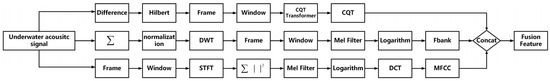
Figure 5.
TriFusion block structure diagram.
3.4.2. TriFusion Block Multi-Dimensional Feature Collaborative Extraction Mechanism
The first branch of the TriFusion block processes the raw acoustic signal using Mel-Frequency Cepstral Coefficients (MFCC). The workflow involves:
- Short-Time Fourier Transform (STFT): Convert the time-domain signal into the frequency domain, yielding spectrogram .
- Mel-Frequency Mapping: Transform linear frequency bins into the Mel scale, aligning with human auditory perception.
- Filter Bank Energy Calculation: Apply a bank of triangular filters to the Mel-scaled spectrum, generating filter bank energies .
- Logarithmic Compression and Discrete Cosine Transform (DCT): Apply logarithmic compression to and perform DCT to derive MFCC features, which emphasize spectral envelope characteristics essential for acoustic pattern discrimination.
This systematic approach ensures the robust extraction of frequency–domain features from the raw signal, laying a critical foundation for the comprehensive multimodal feature fusion framework of the TriFusion block.
Among them, is the audio information, is the Hamming window function, is the frame index, is the frequency index, is the FFT point number (This article is 2048), the number of frame shift points (this article is 512), and the number of Mell filter groups (this article is 128).
The MFCC processing in the TriFusion block captures the dynamic feature variations by emulating human auditory perception. It compresses redundant frequency information, highlights critical spectral components, and enhances steady-state features while suppressing noise interference. Differential calculations further improve sensitivity to temporal changes, providing a stable and robust foundational feature representation for underwater acoustic signals.
In the second part of the TriFusion block, for the differential signal, first, the original audio signal undergoes a first-order difference operation to obtain result . This operation magnifies the instantaneous rate of change and accentuates the high-frequency transient components. Subsequently, the Hilbert transform is applied to extract the envelope, resulting in , which enhances the amplitude variation information. Finally, the Constant-Q Transform (CQT) is employed for time–frequency analysis, generating . The amplitude of is then converted to the dB scale, obtaining .
Among them, is the analysis window function, is the specific frequency point, and ref takes the maximum value of CQT amplitude.
The CQT, with its high-resolution property in the high-frequency band, in combination with the first-order difference and Hilbert envelope, precisely depicts the time–frequency distribution of transient signals such as ship propeller cavitation, thus compensating for the deficiency of MFCC in representing high-frequency dynamic information.
In the third part, for processing the cumulative signal, first, the cumulative sum of the original signal is calculated. This operation smooths out high-frequency fluctuations and highlights the low-frequency trend. Then, the cumulative signal is normalized and subjected to wavelet decomposition to obtain . By taking the approximation coefficients, the low-frequency components are separated, suppressing high-frequency interference. Finally, Fbank features are extracted using a method similar to MFCC, converted to the dB scale to obtain , and the shape is adjusted.
Among them, is the decomposition layer number = 5, is the wavelet coefficient, and is the wavelet basis function.
The Fbank not only preserves the energy distribution and efficiently characterizes the fundamental spectral structure with minimal computational complexity but also retains abundant original acoustic details. It intuitively reflects the energy distribution of audio in the Mel frequency bands, effectively supplementing detailed information in the mid-frequency sub-bands. When integrated with the first two components, it captures full-frequency-band noise information, offering multi-scale feature support.
To visually illustrate the TriFusion block module’s processing of ship-radiated noise signals and feature extraction mechanism, this paper presents six groups of visual spectra (Figure 6). The original signal plot uses time (seconds) as the horizontal axis and amplitude as the vertical axis, intuitively depicting the audio time-domain waveform’s overall trend. The first-order differential signal plot and cumulative signal plot, respectively, show features after differentiation and integration: the former emphasizes signal instantaneous changes, while the latter highlights low-frequency trend components. At the feature spectrum level, the original signal’s MFCC plot reveals the steady-state spectral envelope via Mel-Frequency and time dimensions; the first-order differential signal’s CQT plot with logarithmic frequency and time axes precisely captures the time–frequency distribution of high-frequency transient components; the cumulative signal’s Fbank plot focuses on low-frequency features, presenting the signal’s basic spectral structure under the Mel scale. Figure 6a–f systematically demonstrate the module’s multi-dimensional, multi-level analysis of noise signals—from time-domain waveforms to frequency-domain features, and from original signals to derivative processing results—providing an intuitive basis for understanding the feature extraction mechanism and validating the method’s effectiveness.
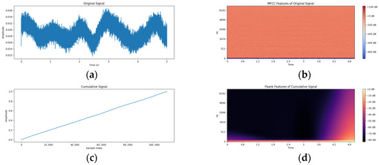

Figure 6.
The processing and feature extraction results of the TriFusion block module on one tug category in the deep ship dataset are presented from different dimensions. (a): Original signal, (b): MFCC of the original signal, (c): Cumulative signal, (d): Fbank of the cumulative signal, (e): First-order difference signal, (f): CQT of the first-order difference signal.
3.4.3. TriFusion Block Feature Fusion
Considering that the MFCC, CQT, and Fbank features extracted by each branch in the TriFusion block initially exist in single-channel forms, each capable of representing ship-radiated noise characteristics from only a single dimension such as steady-state spectral structure (MFCC), high-frequency transient changes (CQT), or low-frequency trends (Fbank), this paper innovatively introduces a multi-channel fusion strategy to expand single-channel features into multi-channel fused features.
Specifically, during the fusion process, these features are arranged in the channel dimension in the order of CQT, MFCC, and Fbank derivative features. Among them, the CQT features, sensitive to high-frequency transient components, can capture the instantaneous high-frequency signals generated by phenomena such as propeller cavitation in ship-radiated noise; the MFCC features, simulating the auditory characteristics of the human ear, effectively characterize the steady-state spectral features of the noise; and the Fbank features focus on low-frequency trends, highlighting low-frequency noise components such as ship mechanical vibrations. Through this arrangement, a fused feature tensor with a shape of 3 × 128 × 216 is finally formed. This fused feature integrates the advantages of different features, enabling collaborative representation of multi-dimensional information in the channel dimension, providing a more discriminative input for the subsequent DART-MT network, contributing to improving the accuracy of ship-radiated noise classification and underwater sonar target recognition.
After the TriFusion block completes feature extraction for the three branches, it integrates different features through a weighted fusion formula as follows:
Among them, , , is the weight coefficient and satisfies .
4. Experimentation
To assess the effectiveness of the DART-MT in real underwater settings, we employed a widely used underwater acoustic dataset to enable comprehensive qualitative and quantitative analyses. This includes comparing DART-MT with current models for underwater acoustic target recognition.
In this section, we present an experimental evaluation of the proposed solution, conducted using three publicly available benchmark datasets with diverse characteristics. We demonstrate the effectiveness of the proposed method and delve into the contributions of each module within DART-MT to gain a deeper understanding of its operational mechanisms. Additionally, we performed several in-depth analyses to address the following research questions (RQs):
RQ1: How does the performance of DART-MT compare to that of SOTA methods in real underwater settings?
RQ2: What is the contribution of the DART-MT key modules to its performance improvement?
RQ3: How effectively does our solution address the challenges described in Section 1 for different datasets?
RQ4: How do DART-MT hyperparameter settings affect recommendation performance?
Most of the comparisons in this study were made with models such as Resnet18, VIT, DenseNet121, and EfficientNetB0 for several reasons. First, these models are widely used in the field of deep learning for various tasks, including image and audio recognition. Their popularity indicates that they have demonstrated good performance in general-purpose feature extraction and classification. Second, they represent different types of neural network architectures. Resnet18 is a classic residual network that effectively addresses the vanishing gradient problem, allowing for deeper network training. VIT, on the other hand, is a Transformer-based model that has shown excellent performance in handling global context information. DenseNet121 has a unique dense connection structure that promotes feature reuse and efficient learning. EfficientNetB0 is designed to balance model complexity and performance, achieving high accuracy with relatively fewer parameters and computational resources. By comparing DART-MT with these models, we can comprehensively evaluate its performance from multiple aspects, including feature extraction ability, model complexity, and generalization performance. This comparison helps to clearly position the DART-MT model in the existing research framework and highlight its advantages and potential areas for improvement.
4.1. Dataset
4.1.1. DeepShip
To systematically evaluate the performance, this study utilized the DeepShip dataset developed by the Northwestern Polytechnical University for underwater acoustic analysis. The dataset comprises recordings of 265 different vessels operating within the Georgia Strait Delta, including cargo ships, passenger liners, oil tankers, and tugboats. These recordings were taken at depths between 141 and 147 m, focusing on vessels within a 2 km radius of the sonar.
The dataset underwent preprocessing, converting all WAV audio files to a consistent 22,050 Hz sampling rate. The underwater acoustic data were divided into 5 s segments, resulting in over 30,000 annotated audio samples. Table 2 provides a detailed description of dataset segmentation.
Table 2.
Details of the four categories in the DeepShip dataset after pre-processing.
4.1.2. ShipsEar
The ShipsEar database, which is a benchmark for underwater acoustic target recognition, is widely used in scientific research. It features noise from the Spanish Atlantic coast, including ship noise and various human-made and natural sounds. The database includes 90 WAV recordings categorized into five classes. Table 3 provides a detailed description of dataset segmentation.
Table 3.
The five classes are included in the ShipsEar database in detail.
The ShipsEar dataset has fewer samples and a more pronounced class imbalance than the DeepShip dataset. This makes ShipsEar more prone to overfitting and challenges in accurately recognizing less-represented classes. Thus, this study focuses on tackling issues of small sample size and class imbalance in the ShipsEar dataset while using the DeepShip dataset to evaluate the generalizability of the modality.
4.1.3. SCTD
To train the model pre-trained weights with a high-resolution underwater acoustic image dataset while maintaining the target confidentiality, the SCTD dataset was utilized in this study. Originally designed for target detection, the SCTD dataset required modifications to suit the underwater acoustic target recognition. These modifications included cropping images to ensure that each contained only one target, and used random cropping and image flipping to increase the sample size and balance categories. The dataset was then divided into training and validation sets in an 8:2 ratio, as shown in Table 4.
Table 4.
Details of the three categories of the SCTD dataset after pre-processing.
4.2. Experimental Settings
The DeepShip dataset encompasses recordings from 265 vessels. After preprocessing, it contains over 30,000 segmented 5 s audio segments, which were partitioned into training, validation, and testing sets at an 8:1:1 ratio. This partitioning strategy ensures a balanced distribution of vessel classes and mitigates overfitting, thereby achieving stable recognition accuracy.
The ShipsEar dataset, preprocessed by standardizing audio to a 22,050 Hz sampling rate and segmenting into 5 s clips, yielded 2223 labeled audio samples. These were split into 1778 training samples and 445 testing samples (8:2 ratio), optimized for the dataset’s class distribution and model evaluation requirements.
During model training, we employed the Lion optimizer with a momentum of 0.9 to reduce noise interference in the input data. The model was trained for 100 epochs with a cosine decay learning rate schedule, starting at 0.0004 to balance convergence speed and stability. A batch size of four was used, and the CB Loss function was applied as the primary evaluation metric. Here, the proportion of labeled samples refers specifically to the ratio of labeled training segments within the training set.
4.3. Evaluation Metrics
A meticulous approach was adopted to minimize inconsistencies across the experiments. This entailed the comprehensive training and assessment of multiple models, accompanied by both qualitative and quantitative assessments of their performance. Extensive comparative studies were conducted to gauge the efficacy of the algorithms.
The computational infrastructure consisted of a Windows 11 operating system, Intel Core i7-12700H processor, 32 gigabytes of random access memory (RAM), NVIDIA GeForce GTX 3070TI graphics processing unit (GPU), and PyTorch version 1.4.0. The subsequent sections delve into the experimental outcomes in greater detail.
The following table outlines the performance indicators used to assess the accuracy of the model. Precision refers to the proportion of genuine positive instances that the classifier accurately identified. Recall measures the fraction of correctly predicted positive cases out of all the actual positive situations. The F1-score, a critical measure in classification tasks, calculates the harmonic mean of the precision and recall. Support signifies the number of samples per class within the validation dataset.
To evaluate the network ability to recognize patterns within a given dataset, we utilized the precision, recall, and F1-score as evaluation metrics. Their mathematical formulations are as follows:
Here, represents the predict the correct answer, stands for the mistakenly predict from other classes to this class, and indicates this category of labels is predicted to be the other category of labels.
4.4. Performance Comparison (RQ1)
4.4.1. Preparation of the Pre-Training Weights
Training with a high-resolution sonar-imaging dataset, such as SCTD, offers foundational knowledge prior to UATR training. For example, sonar imaging provides a wealth of acoustic data, capturing sounds from various angles, distances, and environmental conditions. Utilizing these data to train acoustic models enhances the diversity of the dataset and strengthens the robustness and generalizability of the models. Additionally, applying pre-trained weights from sonar-imaging-trained models enables the transfer of features and knowledge to the sonar-image model. This transfer learning approach can expedite the training of the sonar image model, enhancing its convergence rate and performance. Furthermore, sonar imaging and sonar images share similar physical characteristics and data structures because both are produced through acoustic wave transmission and reception. Thus, employing the pre-trained weights of the sonar imaging model to train the sonar image model can improve its ability to correlate sound with image data. Although the UATR and sonar images in the pre-training set may differ, pre-training serves as an effective starting point for quicker adaptation to underwater sonar images.
Table 5 shows the accuracies of the various models on the SCTD dataset. However, the epoch with the highest recognition rate should not be automatically selected as the optimal pre-trained weight. This caution is due to potential fluctuations in the model recognition rate during training, which means that selecting solely based on the highest rate could result in overfitting. Therefore, we chose the weights with the highest and most stable model accuracy over several epochs as the pre-training weights for future use.
Table 5.
Details of the recognition accuracy of the model on the SCTD dataset.
Table 5 presents the recognition accuracies of different models on the SCTD dataset. The Resnet18 model achieved an accuracy of 0.6481 with a pre-training weight epoch of 56. In comparison, the VIT model achieved an accuracy of 0.8272 in 72 epochs, with an absolute accuracy improvement of 0.1791 over Resnet18. The DenseNet121 model achieved an accuracy of 0.8457 with 50 epochs, showing an absolute improvement of 0.1976 over Resnet18. The EfficientNetB0 model achieved an accuracy of 0.7407 at 25 epochs, having an absolute gain of 0.0926 compared with Resnet18. The DART model exhibited an accuracy of 0.8796 for 60 epochs, with an absolute improvement of 0.2315 over Resnet18.
Models for sonar imaging with limited samples often struggle with learning and generalization during training. Sonar imaging provides a significant amount of acoustic data. By pre-training the models with these data, they can learn essential features and representations from extensive sound datasets. Utilizing these pre-trained weights in the training of sonar-imaging models can enhance learning and generalization, even when samples are scarce. Moreover, pre-training weights offer a favorable starting point, enabling the sonar-image model to converge more quickly and improve the capture of the relationship between sound and image data. This method alleviates the zero-shot problem of models with few samples by using pre-trained knowledge to handle new classes or scenarios without prior training.
Applying pre-trained weights from the SCTD dataset model to the UATR task aids the model in comprehending and analyzing underwater sonar images more effectively. In summary, the initial training of a high-resolution sonar image model provides benefits, including improved feature representation, data augmentation, faster convergence, and parameter initialization. These benefits contribute to enhancing the performance of subsequent sonar-image classification tasks.
4.4.2. Effect of Pre-Trained Weights on Recognition Performance
We employed the pretrained SCTD dataset, a high-resolution sonar-imaging dataset featuring sunken ships, humans, and airplanes, to study model performance. With significant differences in object morphology and application contexts compared to our target UATR (underwater acoustic target recognition of Ships) task, it represents a large domain gap.
Table 6 shows the performance of various models on the ShipsEar sample set, tested with 1%, 5%, and 10% labeled training data, both with and without pre-trained weights. This data demonstrates how models perform when there is a substantial domain difference between pre-trained data and the target task. Analyzing these results reveals model limitations, clarifies their dependence on pre-trained weights, and shows their adaptability in different scenarios. These findings are valuable for improving model performance and guiding model selection in practical applications.
Table 6.
Experiments on whether to incorporate pre-trained weights under 1%, 5%, and 10% training dataset labels in the ShipsEar sample set using different models.
Table 6 demonstrates model performance and the impact of pre-trained weights, particularly under substantial domain gaps between pre-trained data (SCTD: a high-resolution sonar dataset containing sunken ships, humans, and airplanes) and the target UATR ship-recognition task. Without pre-trained weights, DART exhibits moderate performance across 1%, 5%, and 10% label ratios but shows no significant advantage over other models, highlighting limited adaptability to domain shifts in the absence of transfer learning.
Conversely, DART-MT with pre-trained weights achieves dominant performance: at 1% labeling, its accuracy reaches 80.05%, significantly surpassing ResNet18 (59.12%), VIT (56.89%), DenseNet121 (62.05%), and EfficientNetB0 (62.51%). This advantage persists at higher label ratios (89.02% at 5%, 94.86% at 10%), as pre-trained weights—derived from large, feature-rich datasets—enable effective cross-domain feature learning. These results underscore the utility of transfer learning in mitigating small-sample limitations and reducing overfitting risks in data-sparse underwater acoustic recognition tasks.
4.5. Ablation Study (RQ2)
4.5.1. Feature Ablation Experiment
The mean teacher approach is inapplicable to fully labeled data (100% labels), so feature ablation experiments were solely conducted on the DART model. Prior research has validated DART’s effectiveness via its unique architecture and innovative feature-extraction mechanisms, demonstrating its capability to handle complex data patterns and extract discriminative features essential for accurate underwater acoustic target recognition. As an extension of DART, the DART-MT model integrates the mean teacher semi-supervised framework while inheriting DART’s core advantages. DART’s proven feature-extraction capabilities provide a robust foundation for DART-MT, with the added semi-supervised components designed to leverage unlabeled data and further enhance generalization. By optimizing feature learning through the mean teacher framework, DART-MT is expected to build on DART’s strengths, and positive outcomes from DART’s ablation experiments are anticipated to validate DART-MT’s effectiveness in real-world underwater acoustic scenarios.
To assess the characterization capability of the proposed feature extraction methods for raw underwater acoustic signals, Table 7 compares performance across multiple approaches on the ShipsEar dataset: original 2D features, corresponding 3D features, and the 3D feature fusion method described in Section 3.4 of the DART model.
Table 7.
Recognition accuracy of different models with different features on ShipsEar dataset.
Experimental results demonstrate the TriFusion block’s superiority over traditional feature extraction methods across multiple deep learning architectures. When integrated with ResNet variants, TriFusion achieves the highest accuracy: 96.43% for ResNet18, 96.22% for ResNet34, 95.30% for ResNet50, and 94.81% for ResNet101—outperforming MFCC, 3D_MFCC, FBank, and CQT. This highlights TriFusion’s exceptional capability to extract discriminative features from underwater sonar signals.
Similar trends are observed in the EfficientNet series. For example, EfficientNet-B0 achieves 97.10% accuracy with TriFusion, compared to 95.74% for FBank (the second-best performer), with consistent improvements across B1, B2, and B3 variants. This indicates TriFusion’s effectiveness in enhancing feature representation for lightweight architectures.
Notably, TriFusion demonstrates remarkable synergy with the DART model, boosting accuracy to 98.66%—a significant improvement over single features. Even in DenseNet121, TriFusion achieves 97.99% accuracy, outperforming all other methods. These results underscore TriFusion’s versatility in optimizing diverse network architectures, enabling comprehensive capture of acoustic signatures and driving performance gains in underwater acoustic target recognition (UATR).
Compared with single features (e.g., MFCC, FBank, CQT) and simple extensions (e.g., 3D_MFCC), TriFusion’s fused feature design offers distinct advantages. By integrating multi-dimensional information from complementary signal domains, it provides richer, more comprehensive feature representations, thereby significantly enhancing model accuracy in UATR tasks.
While accuracy data enables preliminary assessments, deeper analysis of classification performance requires additional metrics. Confusion matrices and t-SNE plots for ResNet18, EfficientNet-B0, DenseNet121, and DART offer critical insights:
Confusion matrices visually identify misclassification patterns across target categories, exposing weaknesses in feature recognition and decision-making processes.
t-SNE plots project high-dimensional feature vectors into low-dimensional space, enabling visual evaluation of inter-class separability and feature discriminability.
Together, these analyses complement tabular data by providing multi-faceted perspectives on model behavior, facilitating comprehensive and rigorous performance evaluation in UATR tasks.
In the research of underwater acoustic target recognition, we conduct Figure 7 an in-depth analysis of the performance of different models (RESNET18, Efficientnet_B0, Densnet121, DART) on the ShipsEar training dataset through confusion matrices and t-SNE plots, with a particular focus on the superiority of the TriFusion block feature in the DART model.
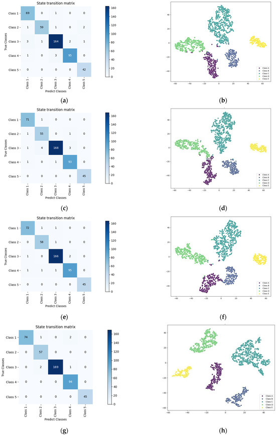
Figure 7.
Confusion matrices and t-SNE diagrams of different models on the ShipsEar training dataset. (a) RESNET18 confusion matrix, (b) t-SNE visualization for the RESNET18 model, (c) the Efficientnet_B0 confusion matrix, (d) t-SNE visualization for the Efficientnet_B0 model, (e) Densnet121 confusion matrix, (f) t-SNE visualization for the Densnet121 model, (g) DART confusion matrix, (h) t-SNE visualization for the DART model.
From the vantage point of the confusion matrix, the DART model exhibits remarkable classification prowess. For example, when examining the confusion matrix of RESNET18 (Figure 7a), while it can achieve a certain number of correct classifications for some classes, there are still instances of misclassification. Certain classes may be confused, resulting in inaccurate predictions for some samples. Similar scenarios are also evident in the confusion matrices of Efficientnet_B0 and Densnet121 (Figure 7c,e), with varying degrees of classification errors. In contrast, the confusion matrix of the DART model (Figure 7g) showcases higher accuracy. Notably, when the TriFusion block feature is employed, the diagonal elements typically have high values. This implies a larger number of correctly classified samples, as the true and predicted classes align closely for each category, significantly reducing misclassifications. Evidently, the TriFusion block feature offers a more accurate classification foundation for the DART model.
The t-SNE plot further uncovers the DART model’s advantage in feature separability. In the t-SNE plots of RESNET18, Efficientnet_B0, and Densnet121 (Figure 7b,d,f), one can observe a certain degree of overlap among different classes. This indicates that the features extracted by these models face challenges in differentiating between classes, suggesting insufficient feature separability. Conversely, in the DART model’s t-SNE plot (Figure 7h), the utilization of the TriFusion block feature leads to a more distinct separation of points belonging to different classes. Each class’s distribution becomes more concentrated, with well-defined boundaries. Visually, this demonstrates the TriFusion block feature’s stronger discriminative power, enabling the DART model to more effectively distinguish various underwater acoustic target classes within the high-dimensional feature space.
To further validate the effectiveness of the TriFusion module in capturing multi-scale acoustic features, we designed a set of quantitative experiments to analyze the contributions of individual features (MFCC from original signals, CQT from differential signals, and FBank from cumulative signals) and their fused representations. Existing studies have shown that single-modality features (such as MFCC for spectral envelopes from original signals, CQT for transient time–frequency analysis from differential signals, and FBank for low-frequency energy characterization from cumulative signals) have limited representational capabilities in complex marine environments, as marine acoustic signals exhibit multi-dimensional coupling characteristics in time-domain dynamics, frequency-domain structures, and energy distributions.
In this experiment, we first extracted MFCC features from original acoustic signals after frame processing, conducted CQT time–frequency analysis on the envelopes of first-order differential signals extracted via Hilbert transform, and extracted FBank features from cumulative signals after wavelet decomposition. These three types of features were then stacked along the channel dimension into a 3 × 128 × 216 tensor to achieve complementary information modeling of time-domain transients, frequency-domain structures, and energy distributions. Based on the DART-MT model architecture and using a semi-supervised learning setup with only 10% labeled data, we compared the performance of single-feature models (MFCC-only from original signals, CQT-only from differential signals, FBank-only from cumulative signals) against the TriFusion module on the ShipsEar dataset. Evaluation metrics included accuracy, F1-scores under class imbalance, and recall rate differences for typical targets.
Combined with the quantitative analysis results of the TriFusion module and single-feature models in Table 8, Figure 8 further presents the confusion matrices of four features (TriFusion block, MFCC-only, CQT-only, Fbank-only) in a visual way, intuitively demonstrating the prediction distribution and error patterns of each model among the five types of samples (Class A to Class E).
Table 8.
Recognition accuracy of different feature map with different features on ShipsEar dataset.
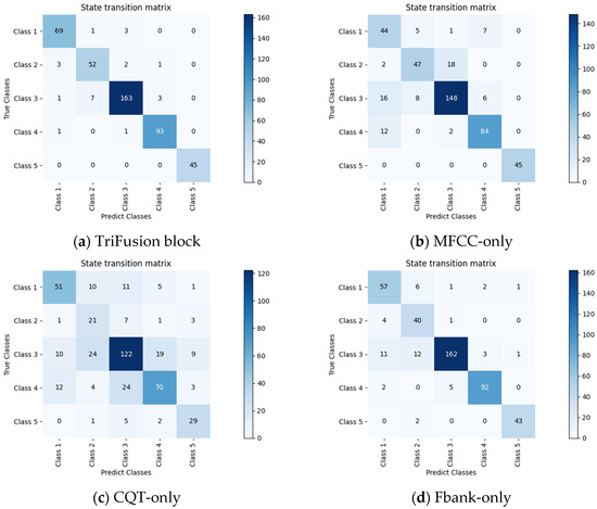
Figure 8.
Confusion Matrices of TriFusion Block, MFCC-only, CQT-only, and Fbank-only Models across Five Classes.
In terms of overall performance, the TriFusion module achieves an average precision, recall, and F1-score of 94.45%, 95.15%, and 94.78%, respectively, significantly outperforming single-feature models such as Fbank-only (85.99%, 89.63%, 87.71%), MFCC-only (82.39%, 83.24%, 82.53%), and CQT-only (62.54%, 66.81%, 63.63%). This indicates that the feature fusion strategy effectively integrates the advantages of different features, particularly demonstrating prominent superiority in complex categories like Class B. The TriFusion achieves an F1-score of 88.14% in Class B, compared to only 45.35% for CQT-only, and 74.01% and 76.19% for MFCC-only and Fbank-only, respectively.
In-depth analysis reveals that MFCC’s lower precision in Class A and Class B may be attributed to insufficient capture of temporal features or limited sensitivity to timbre changes; CQT’s mere 35.00% discriminative ability in Class B highlights its over-reliance on rhythm/pitch features, leading to weak generalization; Fbank’s coexistence of high recall and low precision in Class B indicates its poor discrimination of category boundaries. By contrast, TriFusion forms a multi-dimensional representation by fusing MFCC’s spectral envelope, CQT’s pitch features, and Fbank’s auditory perception features, achieving F1-scores exceeding 88% across all categories and significantly reducing the bias of single features, especially in difficult categories.
The confusion matrix in Figure 8 visually corroborates the above conclusions: TriFusion’s confusion matrix exhibits a higher proportion of diagonal elements, with significantly more correct predictions for each category and a more uniform distribution of off-diagonal errors. In contrast, the confusion matrix of CQT-only in Class B shows frequent errors of misclassifying other categories as Class B through numerous off-diagonal elements, while MFCC-only and Fbank-only display obvious misclassification tendencies due to false negatives and false positives, respectively. This visual analysis concretely demonstrates the practical value of multi-feature fusion in reducing classification bias and improving the accuracy of complex category recognition, providing solid evidence for the application of TriFusion in real-world scenarios.
The underlying reason for this superiority lies in the unique characteristics of the TriFusion block feature. By integrating multiple types of feature information, it can capture the features of underwater acoustic signals more comprehensively and precisely. Compared to the features utilized by other models, the TriFusion block feature can supply the DART model with richer and more representative information, thereby enhancing the model’s performance in classification and feature extraction.
4.5.2. Module Ablation Experiment
To conduct a detailed analysis of the functionality and efficiency of DART-MT, we performed ablation studies on different submodules in DART-MT.
The variant models of DART-MT consist of the following structures. Notations are used only for simplicity.
DART-MT (w/o ResNeXt18), denoted as S1, removes the feature extraction operation using ResNeXt18 in the local feature extraction part and replaces it with a standard convolutional layer for essential feature extraction.
DART-MT (w/o New Transformer Encoder), denoted as S2, removes the multi-head self-attention and related sequence processing operations in the New Transformer Encoder in all corresponding tasks.
DART-MT (w/o CBAM), denoted as S3: Remove the channel and spatial attention mechanisms in the Convolutional Block Attention Module (CBAM).
DART-MT: complete structure of DART-MT.
Table 9 presents ablation study results using precision, recall, and F1-score as evaluation metrics for training and testing on the ShipsEar dataset, with the full DART-MT architecture serving as the baseline. Key findings reveal that each submodule contributes uniquely to model performance:
Table 9.
Ablation experiments of different modules under 50% training dataset labels in the ShipsEar sample set.
ResNeXt18, as the foundational feature extractor employing grouped convolutions, is critical for hierarchical feature representation and fine-grained detail capture. Removing ResNeXt18 (DART-MT → S1) caused significant performance degradation: precision for Class B dropped from 1.00 to 0.72, recall for Class A fell from 0.97 to 0.83, and the average F1-score decreased from 0.9619 to 0.8842. Its absence weakens feature expressiveness, as it adaptively reconstructs information, learns feature interactions, and filters noise from local feature perspectives, enabling subsequent CBAM and New Transformer Encoder modules to access rich input features.
The New Transformer Encoder plays a vital role in capturing global and local sequence context, enhancing holistic semantic understanding. Without it (DART-MT → S2), the F1-score for Class C dropped from 0.96 to 0.93, and the average F1-score fell to 0.9084. While performance declines were less drastic than ResNeXt18’s removal, the module’s ability to model sequential dependencies and contextual relationships remains essential for scenarios where feature order or global structure matters, complementing ResNeXt18’s local feature extraction.
The CBAM attention module optimizes feature discrimination by adaptively weighting channels and spatial locations. In Class E of ShipsEar, CBAM removal (DART-MT → S3) led to a decrease in precision/recall from 1.00 to 0.96, with the average F1-score dropping to 0.9062. By emphasizing task-relevant features and suppressing noise, CBAM enhances representation quality for challenging or imbalanced categories, demonstrating its importance in refining feature saliency and model focus.
In summary, ResNeXt18, New Transformer Encoder, and CBAM form a synergistic architecture: ResNeXt18 excels in local feature discrimination, the New Transformer Encoder enriches global semantic modeling, and CBAM sharpens feature relevance. Their integration enables DART-MT to achieve superior accuracy and expressiveness by addressing multi-scale feature representation, contextual dependencies, and feature saliency simultaneously.
4.6. Discussion of In-Depth Studies (RQ3)
4.6.1. Analysis of Model Performance with Pre-Trained Weights in UATR Task
Although there is a large domain gap between the pre-trained data and the target UATR task, models such as DART-MT with pre-trained weights still show outstanding performance and superiority. This not only highlights the importance of pre-trained weights in improving model accuracy but also suggests that with appropriate pre-training strategies, models can better adapt to tasks with domain gaps and achieve better results.
Comparing Figure 9 and Figure 10 reveals that at 1% labeling, data imbalance causes unrecognized categories in models without pre-trained weights, leading to a zero-shot dilemma. Pretrained weights eliminate this issue: without them, dataset imbalance degrades model accuracy by biasing learning toward overrepresented categories, leaving underrepresented ones poorly recognized.

Figure 9.
Confusion matrix of each model with no pre-trained weight 1% training dataset label. (a) DART; (b) Resnet 18; (c) VIT; (d) DenseNet121; (e) EfficientNetB0.

Figure 10.
Add the confusion matrix of each model under the pre-training weight 1% training dataset label. (a) DART; (b) Resnet 18; (c) VIT; (d) DenseNet121; (e) EfficientNetB0; (f) DART-MT.
Experiments on the ShipsEar dataset with 1%, 5%, and 10% label ratios show the DART model consistently outperforms ResNet18, ViT, DenseNet121, and EfficientNetB0 in recognition accuracy. Adding pre-trained weights to any model not only improves accuracy but also resolves zero-shot issues from sample scarcity. The DART-MT model with pre-trained weights further enhances accuracy compared to the standalone DART model, highlighting its superior effectiveness.
Pre-trained weights mitigate data imbalance by providing models with prior knowledge from large-scale, balanced datasets. This enriches feature representations and optimizes initialization parameters, enabling accurate recognition of underrepresented categories. In semi-supervised UATR with imbalanced samples, pre-trained weights address zero-shot challenges, demonstrating the framework’s transferability.
In summary, DART-MT with pre-trained weights surpasses ViT, ResNet18, DenseNet121, and EfficientNetB0 in recognition accuracy. Its ability to leverage pre-trained knowledge not only resolves small-sample imbalance issues but also exhibits strong transfer learning capabilities, effectively transferring knowledge to new tasks and enhancing recognition performance.
4.6.2. Improvement and Feature Visualization of Models with Limited Labeled Samples
The experimental findings demonstrate the efficacy of the proposed learning framework in enhancing model performance across varying conditions of limited labeled samples. The model reliance on the quantity of labeled samples is significantly diminished. Furthermore, the learning architecture proposed in this study enhances model performance even in scenarios with ample training samples. The experimental results demonstrate that the learning framework can extract information beyond labels, including the essential characteristics and representations of underwater acoustic data.
Additionally, we employed the t-distributed stochastic neighbor embedding (t-SNE) technique to demonstrate enhanced recognition performance and feature separability in models trained with fewer labeled samples. We randomly selected samples from each category of the test dataset. The model was trained on a dataset comprising 10% labeled samples. The learned deep features, represented by the pre-fully connected layer outputs, are shown in Figure 11. A visual comparison of the deep features reveals that within the 10% training dataset, VIT-MT exhibits a substantial overlap in its feature space. Resnet18-MT, DenseNet121-MT, and EfficientNetB0-MT displayed reduced overlap relative to VIT-MT, while DART-MT showed even fewer overlap points and improved category separability, as demonstrated by the features it outputs.
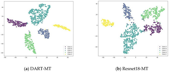
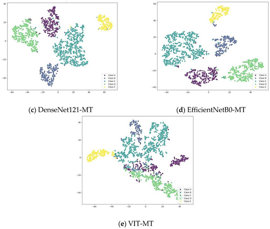
Figure 11.
t-SNE visualization of the output feature vectors of different MT models on the 10% ShipsEar training dataset.
4.6.3. Robustness Analysis and Verification of the Model
In the realm of semi-supervised learning, particularly within the research on the mean teacher framework, two critical issues demand in-depth investigation. First, the mean teacher framework exhibits a strong dependence on unlabeled data, yet the precise influence of variations in data quality and quantity on model performance remains incompletely understood. Given that low-quality data, such as those corrupted by noise, can impede the semi-supervised learning process, elucidating the model’s sensitivity to these data quality changes is of paramount importance. Second, in practical application scenarios—such as underwater environments, which are inherently noisy—existing studies lack comprehensive analyses of model robustness to noise. Understanding how models handle noise is essential for their effective deployment in real-world settings.
To address these research gaps, we employed the ShipsEar dataset with 50% data labeled, systematically introducing varying levels of Gaussian white noise (from −20 dB to 20 dB) to evaluate model performance. This choice of Gaussian white noise—serving as a foundational signal processing benchmark and proxy for underwater thermal noise—enables standardized assessment of noise intensity impacts, though it acknowledges a critical limitation: distinct noise types (e.g., impulsive, pink) may differently affect model predictions, warranting future studies to validate generalizability across diverse noise distributions.
Table 10 presents key performance metrics (accuracy, precision, recall, F1-score) for semi-supervised models—Resnet18-MT, DART-MT, Densenet-MT, EfficientNetB0-MT, VIT-MT—under varying noise levels. These results establish a foundation for analyzing model sensitivity to unlabeled data quality and noise resilience.
Table 10.
Multiple model indicators under different signal-to-noise ratios.
At −20 dB noise, DART-MT achieved 89.02% accuracy, outperforming Resnet18-MT in precision (89.48%, +0.67), recall (89.09%, +0.62), and F1-score (89.28%, +0.64), as well as DenseNet-MT and EfficientNetB0-MT. At −10 dB, DART-MT’s accuracy (80.75%) exceeded Resnet18-MT by 2.07%, with superior recall (80.74%, +1.89) and F1-score (81.86%, +0.83). At 0 dB, DART-MT’s accuracy (90.40%) and all other metrics outperformed competitors, while at 10 dB and 20 dB, it maintained consistent superiority. From −20 dB to 20 dB, DART-MT demonstrated exceptional robustness, with accuracy fluctuations of only 1.57%, far surpassing VIT-MT and other baselines. In underwater scenarios, DART-MT’s ability to mitigate noise-induced degradation and stabilize predictions underscores its superiority in handling low-quality unlabeled data within the mean teacher framework.
Although the model has been tested under different noise levels, the impacts of various types of noise, such as Gaussian noise, white noise, and impulsive noise, on the model may vary significantly. This study only used Gaussian white noise for testing. While it provides a standardized benchmark for evaluating the effects of noise intensity, it is insufficient to fully reflect the model’s robustness in complex real-world environments. For instance, impulsive noise is characterized by suddenness and high energy, which may cause misjudgments in the model. Pink noise, on the other hand, has uneven energy distribution across different frequency bands, and its interference mechanism with the model is entirely different from that of Gaussian white noise. Therefore, future research could introduce multiple types of noise to systematically explore the model’s response differences under various noise distributions, thereby enabling a more accurate assessment of the model’s adaptability to practical applications.
Overall, while our findings validate DART-MT’s robustness to Gaussian white noise, the unaddressed impact of diverse noise types highlights a critical research avenue. Explicitly characterizing noise parameters is imperative for both methodological rigor and practical deployment in noisy environments, positioning DART-MT as a robust choice for semi-supervised learning in complex acoustic settings.
4.6.4. Analysis of the Impact of Different Loss Functions on the Model
As shown in Table 3, there was a significant imbalance between the five categories of the ShipsEar dataset. To solve this problem, a category balance-loss function can be considered. For example, a dynamic category balance-loss function that can adjust the weights based on the changing characteristics of the data can enable the model to adapt to an ever-changing category distribution, thereby providing more accurate predictions. Compared to other methods, the category balance loss function has unique advantages in dealing with such imbalance issues. By reasonably allocating weights to different categories, the model pays sufficient attention to the minority categories and improves their recognition accuracy. Unlike the adaptive sampling technique, which needs to consider the balance between oversampling and undersampling and the possible noise problems introduced, as well as the data augmentation technique, which may cause the model to overfit due to excessive enhancement of the minority categories.
To study the performance of different loss functions in solving the zero-shot problem and handling the sample imbalance in the ShipsEar dataset, we conducted a comparative experiment. The experimental results are listed in Table 11. The experiment used 10% of the labeled data from the ShipsEar dataset. By constructing two new models, DART-MT-CE (using the cross-entropy function) and DART-MT-FL (using the focal loss function),and comparing them with the original DART-MT model (using CB Loss), we can clearly see the differences between different loss functions in handling the sample imbalance problem. In the data preprocessing stage, the selected 10% labeled ShipsEar dataset was processed with the standard audio sampling rate and segmented into 5 s segments. All models were trained according to the training settings of the DART-MT model in the original experiment, keeping parameters such as the momentum, optimizer, number of training epochs, learning rate adjustment strategy, and batch size unchanged. During the training process, changes in the loss value, accuracy, and other indicators of each model were recorded. After the training was completed, the same test set was used to evaluate the performance of the three models on evaluation indicators such as classification accuracy, recall rate, and F1 score. This experiment further verified the effectiveness and advantages of the category balance loss function for handling the sample imbalance problem of the ShipsEar dataset.
Table 11.
Indicators of the DART-MT model under loss functions in the ShipsEar dataset.
By comparing the DART-MT models using different loss functions, we found that DART-MT-CE (using the cross-entropy loss function) performed the worst among all indicators. Although the precision was relatively high, the recall rate was low, resulting in a relatively low F1 score, which is suitable for occasions where high precision is required but the recovery ability is not in high demand. DART-MT-FL (using the focal loss function) showed improvements in all indicators, especially the recall rate and F1 score, indicating that the focal loss function has certain advantages in addressing sample imbalance problems. However, DART-MT (using the Category Balance Loss CB Loss) performed the best for all evaluation indicators, with the highest accuracy, precision, recall, and F1 score. This demonstrates the significant advantage of CB Loss in handling zero-shot learning and solving the problem of sample imbalance. In practical applications, such as underwater acoustic target recognition, sample imbalance and zero-shot learning are common challenges, and CB Loss can better cope with these challenges and improve the performance and generalization ability of the model.
The exploration of different loss functions in this study provides crucial insights into the effectiveness of various loss functions in addressing the complex challenges of sample imbalance and zero-shot learning. The superiority of the CB Loss in the ShipsEar dataset can be attributed to several key factors. First, the CB Loss function is designed to handle the imbalanced distribution of classes by intelligently assigning appropriate weights to different classes. This mechanism ensures that the model pays more attention to minority classes, which are often overlooked in the presence of dominant classes. By doing so, it significantly improves the recognition accuracy of these underrepresented classes.
In the ShipsEar dataset, classes with fewer samples would receive higher weights, compelling the model to learn their unique features more comprehensively. This targeted approach helps balance the learning process and prevents the model from being overly influenced by majority classes. Moreover, CB Loss considers the specific nature of the data distribution and adjusts its weighting scheme to adapt to the specific challenges posed by the dataset. This adaptability makes it highly effective in handling the complex and diverse scenarios encountered in real-world applications.
4.6.5. Analysis of the Computational Complexity and Parameter Quantity of the Model
FLOPs and the number of parameters are vital in model research and evaluation. FLOPs indicate a model computational complexity, helping to assess the operational efficiency of different hardware platforms and select a suitable deployment environment. For example, in high-real-time underwater acoustic target monitoring, lower FLOPs can enhance response speed. The number of parameters is linked to a model complexity and expressiveness. While many parameters can handle complex data, they may cause overfitting with limited data. Studying this number aids in understanding the balance between learning and generalization. Analyzing parameters of various models offers a basis for model selection and improvement. We thus experimented with different models, and the results are shown in Figure 12.
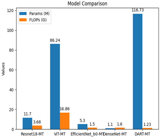
Figure 12.
Params and FLOPs for different models.
The UAPT [51] gives an important foundation and direction for our experiments. Research in underwater acoustic target recognition (UATR) emphasizes the Transformer model advantages. Although it may have more parameters and FLOPs in some cases, this does not undermine its value in marine sonar recognition.
Regarding the number of parameters, a large quantity endows the model with stronger expressiveness. In marine sonar recognition, underwater acoustic signals are complex and diverse, containing various target features and noise. Adequate parameters allow the Transformer model to learn these patterns and better distinguish targets.
DART-MT has unique benefits in terms of the parameters and FLOPs. The parameters are 116.73 M, far exceeding Resnet-18-MT, ViT-MT, EfficientNet_b0-MT, and DenseNet-MT. Despite limited data, its many parameters give strong expressiveness and the ability to learn complex patterns, like a rich “knowledge store” in a small information space, and it uses semi-supervised mean teacher and pre-training transfer methods to enhance generalization and adaptability.
In FLOPs, DART-MT is 1.23 G, lower than other models, needing fewer computing resources for inference, especially useful in resource-limited settings like mobile or edge devices.
Overall, DART-MT parameter advantage helps it handle complex patterns, and its good FLOPs performance balances resource use in training and inference. This may let it outperform others in high-capacity and efficiency-demanding scenarios, though its superiority also depends on factors like architecture, data, training methods, and application scenarios.
4.6.6. Generability Analysis of the Model
In the current field of model research, the evaluation of different model performances is vital. To explore the performance of the various models in practical applications, we conducted a comprehensive comparative experiment. This experiment mainly focused on several key indicators of the models: the accuracy rate, training time, prediction time, and model support. By testing multiple mainstream models, we obtained a set of data with significant reference values, as listed in Table 12.
Table 12.
Training and predicting time.
The DART model outperforms state-of-the-art architectures in multiple key metrics. In terms of classification accuracy, it achieved 98.57 ± 0.031, significantly surpassing ResNet18, Vision Transformer (ViT), DenseNet121, and EfficientNetB0. This high accuracy indicates that DART excels at data classification and prediction tasks, enabling precise target identification. Its performance in fully supervised generalization verification further demonstrates excellent adaptability to diverse datasets, minimizing misclassification errors.
Regarding training efficiency, DART completed training in only 3.100 h, a notable reduction compared to ViT (7.305 h) and DenseNet121 (4.892 h), and shorter than EfficientNetB0 (3.452 h). This shorter training duration accelerates model development, enhancing iteration speed while reducing time and computational costs.
In prediction speed, DART’s 47 s prediction time provides a significant edge over ViT (139 s), DenseNet121 (135 s), EfficientNetB0 (91 s), and ResNet18 (56 s). This rapid prediction capability is crucial for real-time data processing applications, as it enables faster system response and improves overall availability, thus enhancing practical utility.
Given the variability of model performance across different domains, especially in real-world underwater acoustic datasets, investigating the transferability of DART-MT to other datasets is essential. Therefore, we applied the DeepShip dataset and conducted experiments following the procedures described in Section 4.2 and Section 4.3. The detailed experimental results are summarized in Table 13.
Table 13.
Details of the models’ recognition accuracy on the DeepShip dataset.
At a 1% sample label ratio, DART-MT demonstrated a remarkable accuracy of 80.6 ± 0.005%. In contrast, Resnt18-MT achieved an accuracy of 73.2 ± 0.007%, VIT-MT had an accuracy of 66.4 ± 0.010%, DenseNet121-MT reached 69.3 ± 0.008%, and EfficientNetB0-MT obtained 75.2 ± 0.013%. These differences are not only numerically significant but also indicate DART-MT’s superior ability to learn from a minimal amount of labeled data. The asterisks (*) in the table denote that these improvements are statistically significant (p < 0.05), as determined by paired t-tests against the runner-up results. This statistical significance implies that the observed differences in accuracy are not due to random chance but rather reflect the inherent superiority of DART-MT in this low-label-data scenario.
As the sample label ratio increased to 5%, DART-MT’s accuracy rose to 88.2 ± 0.005%, again outperforming the other models. Resnt18-MT reached 82.2 ± 0.004%, VIT-MT achieved 73.4 ± 0.008%, DenseNet121-MT obtained 77.3 ± 0.008%, and EfficientNetB0-MT had an accuracy of 82.9 ± 0.013%. This continued dominance of DART-MT further validates its effectiveness in leveraging additional labeled data for performance improvement.
When the label ratio reached 10%, DART-MT maintained its lead with an accuracy of 96.2 ± 0.005%. Resnt18-MT’s accuracy was 88.9 ± 0.007%, VIT-MT achieved 80.2 ± 0.009%, DenseNet121-MT obtained 82.2 ± 0.010%, and EfficientNetB0-MT had an accuracy of 89.6 ± 0.013%. The significant gap between DART-MT and the other models at this stage indicates that DART-MT can better utilize the increased labeled data to refine its classification capabilities.
At 50% and 90% sample label ratios, DART-MT’s performance continued to excel. With a 50% label ratio, its accuracy was 97.8 ± 0.005%, and at 90%, it reached 98.8 ± 0.004%. The other models, while also showing improvements, lagged far behind. For example, at 90% label ratio, Resnt18-MT had an accuracy of 92.1 ± 0.008%, VIT-MT achieved 87.9 ± 0.010%, DenseNet121-MT obtained 87.8 ± 0.010%, and EfficientNetB0-MT had an accuracy of 93.1 ± 0.013%.
In conclusion, the data in Table 13 clearly demonstrate DART-MT’s robust generalization ability. Its consistent high accuracy across different sample label ratios, especially at lower ratios where data scarcity poses a significant challenge, showcases its effectiveness in handling limited-data scenarios. This superiority over other models in recognizing underwater acoustic targets on the DeepShip dataset positions DART-MT as a promising approach in the field of underwater acoustic target recognition.
Meanwhile, in the literature review, we found that UART [56] can provide favorable initialization for models through pretraining, reduce the risk of falling into local optimality, and demonstrate excellent few-shot classification capabilities. Based on this, we decided to compare the few-shot model with the semi-supervised model DART-MT. Since semi-supervised tasks do not require fully labeled data, Table 14 omits the 100% sample setting. To verify the performance of DART-MT, we compared it with several few-shot models in the table and conducted experiments with labeled data proportions of 1%, 10%, and 50%. These experiments not only proved the adaptability of DART-MT to semi-supervised scenarios but also deeply revealed its unique breakthroughs in improving model accuracy, fully demonstrating its innovative value and superiority over models based on UART’s few-shot capabilities.
Table 14.
Comparison between DART-MT and Few-Shot models on the DeepShip dataset.
In the experiments on the DeepShip dataset, the comparison results between DART-MT and few-shot models fully demonstrate its significant advantages. When the labeled data accounts for only 1%, the accuracy of DART-MT reaches 80.60%, far exceeding that of EncoderA pre-trained with UART (55.26%) and the UART model itself (52.67%), highlighting its outstanding ability to efficiently utilize limited labeled data in extremely data-scarce scenarios. As the proportion of labeled data increases to 10% and 50%, DART-MT still maintains the lead, with accuracies increasing to 96.20% and 97.80%, respectively, which are significantly higher than other models.
This indicates that DART-MT can not only avoid overfitting under low-labeled data but also possesses stronger generalization ability, effectively optimizing model performance by leveraging unlabeled data through semi-supervised learning. Meanwhile, the SCTD pre-trained weights adopted by DART-MT are highly compatible with the semi-supervised strategy, better matching the data distribution in underwater acoustic target recognition tasks. This successfully breaks through the performance bottleneck of few-shot models in data-scarce scenarios, providing a more optimal solution for practical applications.
4.6.7. Comparison Between Fully Supervised and DART-MT Models
From Table 15, the DART-MT model demonstrates outstanding performance in the semi-supervised learning framework, particularly when using different proportions of the training dataset. With only 10% of the training dataset, DART-MT achieves an accuracy of 94.86%, a precision of 94.45%, a recall of 95.15%, and an F1-score of 94.78%. These metrics outperform most fully supervised learning models, such as Yamnet (78.72% accuracy), VGGish (86.75% accuracy), and ADCNN (93.58% accuracy). Although models like CA_MobilenetV2 (98.16% accuracy) and BS-MSF-FAM-scSE (98.40% accuracy) show higher performance with full training data, DART-MT’s ability to leverage a small amount of labeled data combined with abundant unlabeled data in the semi-supervised framework significantly enhances model generalization. This highlights DART-MT’s effectiveness in optimizing recognition performance under limited labeled data conditions.
Table 15.
Comparison results of the evaluated classifiers on the ShipsEar dataset.
Furthermore, the stability of DART-MT is particularly noteworthy. With a standard deviation of merely 0.003 for accuracy and 0.002 for the F1-Score when using 90% of the training dataset, the model exhibits highly consistent performance across experiments, demonstrating strong reliability. Such stability is especially critical in semi-supervised learning, as the inclusion of unlabeled data may introduce noise, and DART-MT effectively addresses this challenge.
In the field of ship radiated noise classification, different models exhibit diverse performances on various datasets. As can be seen from the experimental results of the ShipsEar dataset mentioned above, the DART-MT model demonstrates excellent performance within a semi-supervised learning framework. By efficiently leveraging a small amount of labeled data and a large volume of unlabeled data, it not only outperforms a host of advanced models when using a high proportion of training data but also surpasses most fully supervised learning models when the proportion of training data is low. Moreover, it has remarkable stability. In the research of ship radiated noise, the DeepShip dataset is also an important experimental benchmark. To further explore the generalization ability and adaptability of different models, it is necessary to conduct comparative experiments on the DeepShip dataset using the models that have shown outstanding performance on the ShipsEar dataset. This allows for a more comprehensive evaluation of the actual effectiveness of each model in the task of ship radiated noise classification.
Table 16 presents the performance comparison of various classifiers on the DeepShip dataset. Notably, the DART-MT model demonstrates remarkable superiority even when trained with only 10% of the training dataset. It achieves an accuracy of 96.20%, a precision of 96.23%, a recall of 96.18%, and an F1-score of 96.16%, significantly outperforming many well-known models.
Table 16.
Comparison results of the evaluated classifiers on the DeepShip dataset.
For example, the commonly used Yamnet model only achieves an accuracy of 69.53%, with precision, recall, and F1-score all below 70%. VGGish performs even worse, with an accuracy of 66.85% and other metrics slightly lower. Compared with advanced architectures such as ADCNN (90.23% accuracy) and MobileNetV2 (90.18% accuracy), DART-MT shows a significant improvement of over 6 percentage points. Even when compared with high-performing models like VFR (93.80% accuracy), CA_MobileNetV2 (93.50% accuracy), and BAHTNet (94.57% accuracy), DART-MT surpasses them in overall performance.
This highlights DART-MT’s remarkable ability to effectively utilize limited labeled data in a semi-supervised learning context, demonstrating its strong generalization and adaptability. It serves as a highly competitive and effective solution for ship radiated noise classification on the DeepShip dataset.
In summary, the advantages of DART-MT in semi-supervised learning are multifaceted: it not only achieves performance comparable to or exceeding that of fully supervised learning models with limited labeled data but also further improves its performance as the amount of training data increases, ultimately reaching the highest level among all models. Additionally, its combined strengths in high accuracy, recall, and precision, along with low experimental standard deviations, further validate the effectiveness and robustness of DART-MT within a semi-supervised learning framework. This capability highlights the significant potential of DART-MT in practical applications, particularly in scenarios where labeled data is scarce, as it substantially reduces reliance on large amounts of labeled data while maintaining exceptional performance.
4.6.8. Research on Multi-Scenario Verification of Cross-Environment Adaptability of Marine Acoustic Models
Current research on marine acoustic models predominantly focuses on performance verification under specific environments, with insufficient discussion on adaptability across different sea areas and hydrological conditions (such as ocean currents, temperature, and salinity changes). The complexity of marine environments leads to significant differences in the spectral distribution and intensity dynamic range between inshore ship noise and offshore natural turbulent noise. To fill this research gap, this experiment is based on the ShipsEar dataset and introduces typical environmental noise collected from the South China Sea.
The noise was collected in an area with a water depth of approximately 4000 m, a nearly flat seabed, and sea state level 1 (slight sea, wind speed 1–3 levels). An omnidirectional hydrophone with a sensitivity of −170 dB re 1 V/μPa and a frequency response covering 0.1 Hz to 80 kHz was deployed at a depth of 300 m, combined with a digital acquisition instrument with a sampling frequency of 20 kHz for a high-fidelity collection. The research vessel’s engine was turned off during data collection to eliminate self-noise, ensuring that the original noise only contains natural marine signals such as wave sounds and seabed geological activity noise.
In the experiment, the signal-to-noise ratio (SNR) was systematically controlled to −15 dB, −10 dB, −5 dB, 0 dB, 5 dB, and 10 dB. After dividing the 5 min original noise into 5 s intervals, random noise segments were fused with original audio according to different SNR gradients. Multi-scenario augmented data covering strong noise to clean signals were constructed only in the training set, while the validation set retained original data to objectively evaluate model performance. By comparing the performance of models trained with different SNR augmented data on the original validation set and noise test set, the robustness of target recognition and signal restoration in strong noise scenarios were analyzed.
This study accurately simulates noise changes under typical water depths and hydrological conditions in the South China Sea, which not only systematically verifies the model’s signal extraction capability in deep-sea strong noise environments (such as −15 dB) and recognition effect in inshore complex environments (0 dB to 10 dB) with mixed ship noise and biological signals but also provides key technical support for practical applications of marine acoustic models in cross-sea area acoustic monitoring and underwater target recognition.
Table 17 the DART-MT model demonstrates regular performance changes in South China Sea noise environments with different signal-to-noise ratios (SNRs). When the SNR gradually increases from −15 dB to 5 dB, the model’s accuracy rises from 91.49% to 93.53%, with the F1-Score peaking at 93.62% at 5 dB, indicating the most balanced signal extraction and recognition under moderate noise conditions. However, when the SNR further increases to 10 dB, the accuracy drops to 92.39%, possibly due to differences in noise spectral characteristics and training data distribution at high SNRs, leading to fluctuations in generalization ability. It is worth noting that the model still maintains an accuracy of over 91% in the strong noise environment of −15 dB, and the standard deviation of all indicators is less than 0.02, verifying its stability under extreme noise. In the noise-free scenario, the model’s accuracy reaches 94.86%, with a difference of only 1.33% from the 5 dB scenario, indicating strong noise resistance.
Table 17.
The accuracy, precision, recall, and F1-score of DART-MT in the signal-to-noise ratio range from −15 dB to 10 dB.
To deeply analyze the model’s classification performance across different categories and noise conditions, Figure 13 presents the confusion matrices of the DART-MT model under various signal-to-noise ratio (SNR) scenarios. In contrast to the macro statistics of overall accuracy, precision, recall, and F1-score in the previous table, these matrices offer a fine-grained perspective on the model’s classification details for each category—clearly revealing which acoustic signal categories are more prone to misjudgment in specific noise environments.
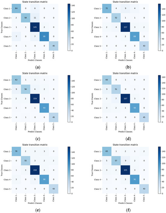
Figure 13.
The confusion matrices of the DART-MT model under the training dataset with 10% labeled data from pre-trained weights and mixed South China Sea noise at different signal-to-noise ratios (SNRs). (a) −15 dB; (b) −10 dB; (c) −5 dB; (d) 0 dB; (e) 5 dB; (f) 10 dB.
Although the current experiment covers a wide range of SNRs, there are still limitations in the research on marine environmental adaptability. On the one hand, it only simulates environmental changes by controlling noise intensity, without involving the impact of different sea areas (such as inshore and offshore), seabed topography (reef areas and plains), or hydrological parameters (ocean currents, salinity) on noise characteristics. For example, the spectral differences between low-frequency turbulent noise in the deep South China Sea and high-frequency ship noise in inshore areas are not distinguished. On the other hand, the noise source is single, lacking the simulation of mixed scenarios of multi-source noise such as biological sonar and industrial noise, making it difficult to fully reflect the complexity of the real marine environment.
Future research can be expanded from multiple dimensions: introducing noise data from different sea areas and water depths to build a cross-environment database, and analyzing the model’s adaptability in scenarios with significant spectral feature differences; combining the physical impact of parameters such as temperature and salinity on sound propagation, and simulating signal transmission under different hydrological conditions through data augmentation; designing multi-source noise mixing experiments, such as superimposing ship, biological, and geological activity noise in proportion, to evaluate the model’s target recognition ability in complex scenarios such as inshore ports and offshore fishing grounds. These studies will significantly enhance the model’s cross-environment adaptability in practical applications such as deep-sea detection and inshore monitoring, providing more transferable technical solutions for global marine acoustic monitoring networks.
4.7. Hyper-Parameter Analysis (RQ4)
This study compares the proposed training framework with typical Resnet, VIT, DenseNet121, and EfficientNetB0 models for underwater target recognition using the mean teacher learning framework. During the self-supervised learning phase, all samples were treated as unlabeled, without using label information. In the supervised fine-tuning phase, the model loads the previously trained weights and fine-tunes various sample sizes. The training parameters during the supervised fine-tuning phase were aligned with those in the baseline experiment. Following supervised fine-tuning, training progressed to the semi-supervised fine-tuning phase with label ratios of 1%, 5%, 10%, 50%, and 90% in the training set. Ultimately, all models underwent training on all unlabeled samples using unsupervised self-distillation. The training process ensures that the model accesses only partial label information specified by the training dataset.
Table 18 shows that across all label ratios, the models employing the mean teacher learning strategy significantly outperformed those that did not. This suggests that the mean teacher training strategy effectively enhanced model performance. Under the mean teacher-training strategy, the student model boosts its generalization performance by jointly training with the teacher model through a blend of supervised and unsupervised learning. The teacher model created pseudo-labels for unlabeled data, which were then used to train the student model. Consistency constraints between student and teacher models allow for a better understanding of data characteristics and patterns, thus enhancing performance. Models leveraging the mean teacher strategy attained a higher accuracy across different label ratios. Notably, at lower label ratios, the DART-MT model showed a more significant performance improvement than the other models. Consequently, by integrating the mean teacher strategy, the DART-MT model makes better use of limited labeled data to enhance performance and allows the student model to leverage the teacher model knowledge for improved generalization.
Table 18.
Recognition accuracy of different training dataset label ratios and different models in the ShipsEar dataset.
Figure 14 shows that model accuracy increases with the training label ratio, as models can learn from more labeled samples to optimize performance. For instance, the DART-MT model accuracy goes from 0.800 at a 1% ratio to 0.8907 at 5%, indicating that severely limited labeled samples impede comprehensive learning and generalization, thus restricting performance. When the ratio rises from 10% to 50%, DART-MT accuracy improves from 0.9486 to 0.9645, thanks to better utilization of labeled-sample information. Notably, from 50% to 90%, DART-MT accuracy sees a 2.4% increase, from 0.9645 to 0.9885. This relatively modest rise might be due to the model already having sufficient labeled data at higher ratios, where additional increases yield only marginal performance gains. Overall, the training label ratio significantly affects model accuracy: increasing it within a certain range enhances performance, but beyond that point, improvements are minimal, and low ratios constrain performance. Therefore, choosing an appropriate label ratio requires balancing data-collection costs and potential performance enhancements.
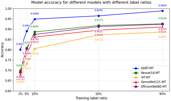
Figure 14.
Precision plots of different models in different ShipsEar training dataset label proportions.
Figure 15 illustrates that with 10% training labels, both training and validation losses decreased notably within the initial 12 epochs, suggesting effective feature and pattern learning by the model. Subsequently, both the training and validation losses stabilized without further decrease and fluctuated within a defined range. Observing the evolution of the training and validation losses reveals a relatively small gap between them, signifying the model’s strong generalization capability. Consequently, with such a small gap, the generalization ability of the model can be deemed acceptable.

Figure 15.
Changes in the loss function during the 10% ShipsEar training dataset label DART-MT training process.
Figure 16 presents the changes in the model precision, recall rate, and accuracy with the number of training epochs. When the training was about 10 epochs, the fluctuations of the three metric curves decreased and tended to stabilize. The model began to converge and its performance became stable. After convergence, the precision was nearly 0.95, with few misjudgments; the recall rate was about 0.95, with few positive examples missed; and the accuracy also remained high, indicating a good classification effect on both positive and negative samples. The model could converge in about 10 epochs, thanks to the good parameter initialization starting point provided by the pre-trained weights, avoiding the long-term oscillations and convergence difficulties that might be caused by random initialization. Moreover, the precision, recall rate, and accuracy remained at a high level after convergence, indicating that the pre-trained weights enabled the model to utilize the general features obtained from large-scale pre-training to capture the data patterns of the current task more quickly. Judging from the convergence speed and the final metric performance, the pre-trained weights most likely played a positive role.
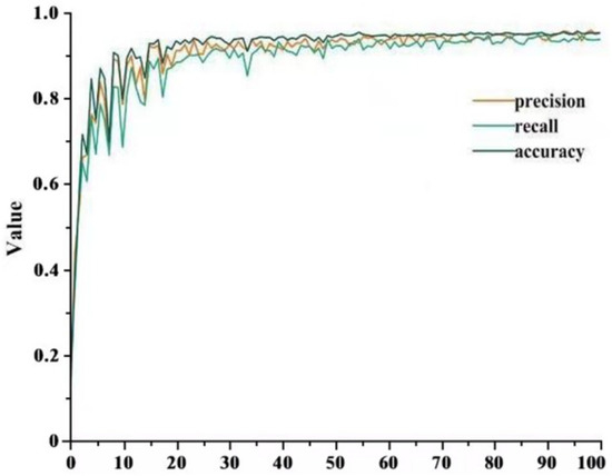
Figure 16.
Variation plot of precision, recall, and accuracy during the training process of DART-MT with 10% of the ShipsEar training dataset labels.
4.8. Discussions and Analysis
The learning framework proposed in this study effectively enhances the model performance, even with few labeled and many unlabeled samples. We attribute this improvement to the comprehensive use of an extensive unlabeled sample set. The mean teacher model utilizes unlabeled data for self-training, thus playing a vital role in semi-supervised learning to enhance the model generalization and performance. A major advantage of incorporating unlabeled data is the expansion of the training dataset compared with the use of solely labeled data. Unlabeled data serve as additional training samples that offer informative signals. Leveraging unlabeled data enables the model to learn robust feature representations and improve prediction accuracy. Furthermore, unlabeled data help stabilize the training process. In the mean teacher model, there is a distinction between the teacher and student networks. The teacher network generates stable targets by averaging the predictions across various perturbations, such as data augmentation. The use of unlabeled data diversifies these perturbations, boosting the robustness and generalizability of the model. By harnessing unlabeled data for self-supervision and semi-supervision, the mean teacher model achieved superior performance, generalization, and predictive outcomes with few labeled samples.
A poorly performing teacher network inevitably limits the student network performance, aligning with the no-free-lunch theorem. Without sufficient information to guide the learning, the model struggles to perform well. The suggested learning framework and semi-supervised fine-tuning method somewhat enhance the constraints on the model learning. Introducing pre-trained weights to the mean teacher model helps it converge more quickly to the optimal solution during training. This efficiency is due to the pre-trained weights being developed on large-scale datasets, which endow them with robust feature representation abilities. Utilizing pre-trained weights, the teacher model learns general or advanced features from prior tasks and fine-tunes them for specific tasks, thereby enhancing its performance. With limited training data, pre-trained weights leverage existing knowledge and mitigate the risk of overfitting owing to data scarcity. Additionally, the multistage learning framework extends the total training duration beyond that of traditional supervised training. However, the time investment in this learning framework is minimal compared with the extensive effort required to annotate large datasets manually. Labeling the entire dataset typically requires months. The proposed learning framework saves significant time in labeling and reduces the likelihood of errors in dataset annotations. For instance, the DART-MT model achieved comparable or superior results to fully supervised models with only 10% of the labeled dataset.
5. Conclusions
This study addresses the challenges in the field of underwater acoustic target recognition (UATR), such as difficult data annotation, sample imbalance, and insufficient traditional feature extraction, especially in complex scenarios with a large number of unlabeled samples and a small number of labeled samples. A DART-MT model is proposed. This model uses an innovative semi-supervised pre-training method to transfer knowledge from a pre-trained “teacher” model to a “student” model, significantly alleviates the zero-shot recognition problem in imbalanced and small-sample scenarios.
In the DART-MT model, the TriFusion Block plays a crucial role. It is a novel feature fusion architecture that simultaneously processes raw, differential, and cumulative acoustic signals to extract MFCC, CQT, and FBank features, respectively. This process constructs a 3 × 128 × 216 tensor that comprehensively captures the multi-scale characteristics of underwater acoustic signals. Compared with traditional single-feature extraction methods, the TriFusion Block can obtain signal information from different dimensions, effectively compensating for the limitations of conventional approaches. It provides a richer and more representative feature foundation for subsequent feature analysis and classification, thereby significantly enhancing the model’s ability to understand and process complex underwater acoustic signals. This makes a key contribution to improving the overall performance of the DART-MT model.
The experimental results strongly demonstrate the excellent performance of the DART-MT model. Tests on the DeepShip and ShipsEar datasets show that when 10% labeled data are used, the accuracy of the DART-MT model reaches 96.20% on the DeepShip dataset and 94.86% on the ShipsEar dataset. When the labeled data are increased to 90%, the accuracy on the DeepShip dataset is as high as 98.8%, and on the ShipsEar dataset it reaches 98.85%. Its performance is comparable to or even better than fully supervised models, fully demonstrating its ability to overcome the limitations of scarce annotation resources and perform stably under different labeling ratios.
Ablation experiments further verify the effectiveness and wide applicability of the proposed semi-supervised learning method. By optimizing the loss function of the student model, especially when dealing with the sample imbalance problem in the ShipsEar dataset, the CB Loss function used has significant advantages over other loss functions, significantly improving the recognition accuracy of minority classes and enhancing the model performance.
In terms of noise resistance, taking the ShipsEar dataset as an example, under different noise levels from −20 dB to 20 dB, the DART-MT model significantly outperforms other comparative models in terms of accuracy, precision, recall, and F1-score. Moreover, its performance fluctuations are minimal, showing strong noise-resistant robustness and enabling stable and accurate results in complex noisy environments. In addition, the DART-MT model has unique advantages in terms of parameters and computational complexity. Its 116.73M parameters endow the model with a strong ability to learn complex patterns, while its 1.23G FLOPs ensure low computational resource requirements during inference, making it suitable for resource-constrained application scenarios.
Looking ahead, the research will focus on leveraging unlabeled data to impose more constraints during training, further reducing the model’s dependence on labeled samples and enhancing its performance in data-scarce scenarios. At the same time, different architectures of the teacher and student models will be explored, and in-depth research on the impact of network configurations on the behavior and effectiveness of the DART-MT model will be conducted to continuously optimize semi-supervised learning in underwater acoustics and enable it to better address various challenges in the real world.
Author Contributions
G.X.: Writing—original draft, Software, Validation, Formal analysis. Z.C.: Methodology, Project administration, Resources, Supervision, Writing—review and editing. Y.L.: Writing—review and editing, Supervision. M.C.: Formal analysis, Investigation, Software, Validation. F.C.: Formal analysis, Investigation. Y.Z.: Supervision, Project administration. H.J.: Funding acquisition, Visualization. H.Q.: Resources, Funding acquisition. All authors have read and agreed to the published version of the manuscript.
Funding
This work is supported by the Guangxi Special Program for Technological Innovation Guidance under Grant No. GuiKeAC25069006, and Guangxi Natural Science Foundation under Grant No. 2024GXNSFBA010144.
Data Availability Statement
Data will be made available on request.
Conflicts of Interest
The authors declare that they have no known competing financial interests or personal relationships that could have appeared to influence the work reported in this paper.
References
- Talaei Khoei, T.; Ould Slimane, H.; Kaabouch, N. Deep learning: Systematic review, models, challenges, and research directions. Neural Comput. Appl. 2023, 35, 23103–23124. [Google Scholar] [CrossRef]
- Mu, R.; Zeng, X. A review of deep learning research. KSII Trans. Internet Inf. Syst. (TIIS) 2019, 13, 1738–1764. [Google Scholar] [CrossRef]
- Lei, Z.; Lei, X.; Wang, N.; Zhang, Q. Present status and challenges of underwater acoustic target recognition technology: A review. Front. Phys. 2022, 10, 1044890. [Google Scholar] [CrossRef]
- Feng, S.; Ma, S.; Zhu, X.; Yan, M. Artificial Intelligence-Based Underwater Acoustic Target Recognition: A Survey. Remote Sens. 2024, 16, 3333. [Google Scholar] [CrossRef]
- Luo, X.; Chen, L.; Zhou, H.; Cao, H. A survey of underwater acoustic target recognition methods based on machine learning. J. Mar. Sci. Eng. 2023, 11, 384. [Google Scholar] [CrossRef]
- Wang, J.; Li, J.; Yan, S.; Shi, W.; Yang, X.; Guo, Y.; Gulliver, T.A. A Novel Underwater Acoustic Signal Denoising Algorithm for Gaussian/Non-Gaussian Impulsive Noise. IEEE Trans. Veh. Technol. 2021, 70, 429–445. [Google Scholar] [CrossRef]
- Domingos, L.C.; Santos, P.E.; Skelton, P.S.; Brinkworth, R.S.; Sammut, K. A survey of underwater acoustic data classification methods using deep learning for shoreline surveillance. Sensors 2022, 22, 2181. [Google Scholar] [CrossRef]
- Tian, S.; Chen, D.; Wang, H.; Liu, J. Deep convolution stack for waveform in underwater acoustic target recognition. Sci. Rep. 2021, 11, 9614. [Google Scholar] [CrossRef] [PubMed]
- Neupane, D.; Seok, J. A Review on Deep Learning-Based Approaches for Automatic Sonar Target Recognition. Electronics 2020, 9, 1972. [Google Scholar] [CrossRef]
- Zhu, C.; Cao, T.; Chen, L.; Dai, X.; Ge, Q.; Zhao, X. High-order domain feature extraction technology for ocean acoustic observation signals: A review. IEEE Access 2023, 11, 17665–17683. [Google Scholar] [CrossRef]
- Yao, Q.; Wang, Y.; Yang, Y. Underwater acoustic target recognition based on data augmentation and residual CNN. Electronics 2023, 12, 1206. [Google Scholar] [CrossRef]
- Zhu, X.; Dong, H.; Rossi, P.S.; Landrø, M. Time-frequency fused underwater acoustic source localization based on contrastive predictive coding. IEEE Sens. J. 2022, 22, 13299–13308. [Google Scholar] [CrossRef]
- Han, R.; Jia, N.; Huang, J.; Guo, S. Joint time-frequency domain equalization of MSK signal over underwater acoustic channel. Appl. Acoust. 2022, 189, 108597. [Google Scholar] [CrossRef]
- Liu, Z.; Peng, D.; Zuo, M.J.; Xia, J.; Qin, Y. Improved Hilbert–Huang transform with soft sifting stopping criterion and its application to fault diagnosis of wheelset bearings. ISA Trans. 2022, 125, 426–444. [Google Scholar] [CrossRef]
- Tian, C.; Zheng, M.; Zuo, W.; Zhang, B.; Zhang, Y.; Zhang, D. Multi-stage image denoising with the wavelet transform. Pattern Recognit. 2023, 134, 109050. [Google Scholar] [CrossRef]
- Di, N.; Sharif, M.Z.; Hu, Z.; Xue, R.; Yu, B. Applicability of VGGish embedding in bee colony monitoring: Comparison with MFCC in colony sound classification. PeerJ 2023, 11, e14696. [Google Scholar] [CrossRef]
- Zhou, C.; Wu, Y.; Fan, Z.; Zhang, X.; Wu, D.; Tao, Z. Gammatone spectral latitude features extraction for pathological voice detection and classification. Appl. Acoust. 2022, 185, 108417. [Google Scholar] [CrossRef]
- Ali, S.; Iqbal, N.; Hafeez, Y. Towards requirement change management for global software development using case base reasoning. Mehran Univ. Res. J. Eng. Technol. 2018, 37, 639–652. [Google Scholar] [CrossRef]
- Linka, K.; Kuhl, E. A new family of Constitutive Artificial Neural Networks towards automated model discovery. Comput. Methods Appl. Mech. Eng. 2023, 403, 115731. [Google Scholar] [CrossRef]
- Xiao, X.; Wang, W.; Ren, Q.; Gerstoft, P.; Ma, L. Underwater acoustic target recognition using attention-based deep neural network. JASA Express Lett. 2021, 1, 106001. [Google Scholar] [CrossRef]
- Li, J.; Wang, B.; Cui, X.; Li, S.; Liu, J. Underwater acoustic target recognition based on attention residual network. Entropy 2022, 24, 1657. [Google Scholar] [CrossRef]
- Yang, S.; Xue, L.; Hong, X.; Zeng, X. A lightweight network model based on an attention mechanism for ship-radiated noise classification. J. Mar. Sci. Eng. 2023, 11, 432. [Google Scholar] [CrossRef]
- Qi, Z.; Li, T.; Chen, J.; Yam, J.C.; Wen, Y.; Huang, G.; Zhong, H.; He, M.; Zhu, D.; Dai, R.; et al. A deep learning system for myopia onset prediction and intervention effectiveness evaluation in children. npj Digit. Med. 2024, 7, 206. [Google Scholar] [CrossRef]
- Sheng, B.; Pushpanathan, K.; Guan, Z.; Lim, Q.H.; Lim, Z.W.; Yew, S.M.E.; Goh, J.H.L.; Bee, Y.M.; Sabanayagam, C.; Sevdalis, N.; et al. Artificial intelligence for diabetes care: Current and future prospects. Lancet Diabetes Endocrinol. 2024, 12, 569–595. [Google Scholar] [CrossRef]
- Li, J.; Guan, Z.; Wang, J.; Cheung, C.Y.; Zheng, Y.; Lim, L.L.; Lim, C.C.; Ruamviboonsuk, P.; Raman, R.; Corsino, L.; et al. Integrated image-based deep learning and language models for primary diabetes care. Nat. Med. 2024, 30, 2886–2896. [Google Scholar] [CrossRef] [PubMed]
- Ali, S.G.; Wang, X.; Li, P.; Li, H.; Yang, P.; Jung, Y.; Qin, J.; Kim, J.; Sheng, B. EGDNet: An efficient glomerular detection network for multiple anomalous pathological feature in glomerulonephritis. Vis. Comput. 2024, 41, 2817–2834. [Google Scholar] [CrossRef]
- Dai, L.; Wu, L.; Li, H.; Cai, C.; Wu, Q.; Kong, H.; Liu, R.; Wang, X.; Hou, X.; Liu, Y.; et al. A deep learning system for detecting diabetic retinopathy across the disease spectrum. Nat. Commun. 2021, 12, 3242. [Google Scholar] [CrossRef]
- Zhang, W.; Yu, P.; Wang, Z.; Wang, Z.; Xu, M. A hybrid offline-online method for sound event localization and detection. Appl. Intell. 2024, 54, 11357–11372. [Google Scholar] [CrossRef]
- Ren, J.; Xie, Y.; Zhang, X.; Xu, J. UALF: A learnable frontend for intelligent underwater acoustic classification system. Ocean Eng. 2022, 264, 112394. [Google Scholar] [CrossRef]
- Doan, V.-S.; Huynh-The, T.; Kim, D.-S. Underwater Acoustic Target Classification Based on Dense Convolutional Neural Network. IEEE Geosci. Remote Sens. Lett. 2020, 19, 1500905. [Google Scholar] [CrossRef]
- Khishe, M. DRW-AE: A Deep Recurrent-Wavelet Autoencoder for Underwater Target Recognition. IEEE J. Ocean. Eng. 2022, 47, 1083–1098. [Google Scholar] [CrossRef]
- Santos-Domínguez, D.; Torres-Guijarro, S.; Cardenal-López, A.; Pena-Gimenez, A. ShipsEar: An underwater vessel noise database. Appl. Acoust. 2016, 113, 64–69. [Google Scholar] [CrossRef]
- Feng, S.; Zhu, X. A transformer-based deep learning network for underwater acoustic target recognition. IEEE Geosci. Remote Sens. Lett. 2022, 19, 1–5. [Google Scholar] [CrossRef]
- Irfan, M.; Zheng, J.; Ali, S.; Iqbal, M.; Masood, Z.; Hamid, U. DeepShip: An underwater acoustic benchmark dataset and a separable convolution based autoencoder for classification. Expert Syst. Appl. 2021, 183, 115270. [Google Scholar] [CrossRef]
- Wang, Q.; Wang, L.; Zeng, X.Y. An improved deep clustering model for underwater acoustical targets. Neural Process. Lett. 2018, 48, 1633–1644. [Google Scholar] [CrossRef]
- Hu, G.; Wang, K.J.; Peng, Y. Deep learning methods for underwater target feature extraction and recognition. Comput. Intell. Neurosci. 2018, 2018, 1214301. [Google Scholar] [CrossRef] [PubMed]
- Hu, G.; Wang, K.J.; Liu, L.L. Underwater acoustic target recognition based on depthwise separable convolution neural networks. Sensors 2021, 21, 1429. [Google Scholar] [CrossRef]
- Testolin, A.; Diamant, R. Combining denoising autoencoders and dynamic programming for acoustic detection and tracking of underwater moving targets. Sensors 2020, 20, 2945. [Google Scholar] [CrossRef]
- Xue, L.Z.; Zeng, X.Y. Underwater acoustic target classification based on u-shaped network. In Proceedings of the INTER-NOISE and NOISE-CON Congress and Conference Proceedings, InterNoise21, Washington, DC, USA, 1–5 August 2021; pp. 970–1944, 1338–1345. [Google Scholar] [CrossRef]
- He, K.; Fan, H.; Wu, Y.; Xie, S.; Girshick, R. Momentum contrast for unsupervised visual representation learning. In Proceedings of the IEEE Conference on Computer Vision and Pattern Recognition, Seattle, WA, USA, 13–19 June 2020; pp. 9729–9738. [Google Scholar] [CrossRef]
- Wang, H.; Tian, S.Z.; Fu, Y.; Zhou, J.L.; Liu, J.F.; Chen, D.B. Feature augmentation based on information fusion rectification for few-shot image classification. Sci. Rep. 2023, 13, 3607. [Google Scholar] [CrossRef]
- Tian, S.Z.; Bai, D.; Zhou, J.L.; Fu, Y.; Chen, D.B. Few-shot learning for joint model in underwater acoustic target recognition. Sci. Rep. 2023, 13, 17502. [Google Scholar] [CrossRef]
- Ghavidel, M.; Azhdari, S.M.H.; Khishe, M.; Kazemirad, M. Sonar data classification by using few-shot learning and concept extraction. Appl. Acoust. 2022, 195, 108856. [Google Scholar] [CrossRef]
- Sohn, K.; Berthelot, D.; Carlini, N.; Zhang, Z.; Zhang, H.; Raffel, C.A.; Li, C.L. Fixmatch: Simplifying semi-supervised learning with consistency and confidence. Adv. Neural Inf. Process. Syst. 2020, 33, 596–608. [Google Scholar] [CrossRef]
- Li, J.; Wu, X. Simple framework for the contrastive learning of visual representations-based data-driven tight frame for seismic denoising and interpolation. GEOPHYSICS 2022, 87, V467–V480. [Google Scholar] [CrossRef]
- Hong, F.; Liu, C.W.; Guo, L.J.; Chen, F.; Feng, H. Underwater acoustic target recognition with a residual network and the optimized feature extraction method. Appl. Sci. 2021, 11, 1442. [Google Scholar] [CrossRef]
- Li, J.H.; Yang, H.H. The underwater acoustic target timbre perception and recognition based on the auditory inspired deep convolutional neural network. Appl. Acoust. 2022, 182, 108210. [Google Scholar] [CrossRef]
- Jia, H.L.; Khishe, M.; Mohammadi, M.; Rashidi, S. Deep cepstrum-wavelet autoencoder: A novel intelligent sonar classifier. Expert Syst. Appl. 2022, 202, 117295. [Google Scholar] [CrossRef]
- Zhou, T.F.; Bredell, G.; Li, L.L.; Li, J.; Unkelbach, J.; Konukoglu, E. Volumetric memory network for interactive medical image segmentation. Med. Image Anal. 2023, 83, 102599. [Google Scholar] [CrossRef]
- Fayaz, S.; Parah, S.A.; Qureshi, G.J. Underwater object detection: Architectures and algorithms—A comprehensive review. Multimed. Tools Appl. 2022, 81, 20871–20916. [Google Scholar] [CrossRef]
- Tang, J.; Ma, E.; Qu, Y.; Gao, W.; Zhang, Y.; Gan, L. UAPT: An Underwater Acoustic Target Recognition Method Based on Pre-trained Transformer. Res. Sq. 2024. preprint. [Google Scholar] [CrossRef]
- He, K.; Zhang, X.; Ren, S.; Sun, J. Deep residual learning for image recognition. In Proceedings of the IEEE Conference on Computer Vision and Pattern Recognition, Las Vegas, NV, USA, 27–30 June 2016; pp. 770–778. [Google Scholar] [CrossRef]
- Dosovitskiy, A.; Beyer, L.; Kolesnikov, A.; Weissenborn, D.; Zhai, X.; Unterthiner, T.; Dehghani, M.; Minderer, M.; Heigold, G.; Gelly, S.; et al. An image is worth 16x16 words: Transformers for image recognition at scale. arXiv 2020, arXiv:2010.11929. [Google Scholar] [CrossRef]
- Iandola, F.; Moskewicz, M.; Karayev, S.; Girshick, R.; Darrell, T.; Keutzer, K. Densenet: Implementing efficient convnet descriptor pyramids. arXiv 2014, arXiv:1404.1869. [Google Scholar] [CrossRef]
- Koonce, B. Convolutional Neural Networks with Swift for Tensorflow: Image Recognition and Dataset Categorization; Apress: Berkeley, CA, USA, 2021. [Google Scholar] [CrossRef]
- Xie, Y.; Ren, J.; Xu, J. Underwater-art: Expanding information perspectives with text templates for underwater acoustic target recognition. J. Acoust. Soc. Am. 2022, 152, 2641–2651. [Google Scholar] [CrossRef] [PubMed]
- Tsai, Y.S.; Fang, Y.Y.; Chen, C.F.; Tsai, M.F.; Weng, S.H.; Kuo, T.J. Recognition and classification of ship noise in underwater soundscape based on yet another mobile network and unmanned surface vehicle. In Proceedings of the 2025 IEEE Underwater Technology (UT), Taipei, Taiwan, 2–5 March 2025. [Google Scholar] [CrossRef]
- Yu, X.; Li, S.; Ning, J.; Li, D. A target recognition method of underwater acoustic signal based on VGGis h neural network model. Tech. Acoust. 2024, 43, 30–37. [Google Scholar] [CrossRef]
- Yang, H.H.; Li, J.H.; Shen, S.; Xu, G.H. A deep convolutional neural network inspired by auditory perception for underwater acoustic target recognition. Sensors 2019, 19, 1104. [Google Scholar] [CrossRef]
- Liu, F.; Shen, T.; Luo, Z. Underwater target recognition using convolutional recurrent neural networks with 3-D Mel-spectrogram and data augmentation. Appl. Acoust. 2021, 178, 107989. [Google Scholar] [CrossRef]
- Han, X.C.; Ren, C.; Wang, L.; Bai, Y. Underwater acoustic target recognition method based on a joint neural network. PLoS ONE 2022, 17, e0266425. [Google Scholar] [CrossRef]
- Li, M.; Li, J.; Feng, H. Detection and recognition of underwater acoustic communication signal under ocean back ground noise. IEEE Access 2024, 12, 149432–149446. [Google Scholar] [CrossRef]
- Huang, Y.; Guo, T.; Wang, H.; Wu, Y.; Chen, X. Mobile_ViT: Underwater Acoustic Target Recognition Method Based on Local–Global Feature Fusion. J. Mar. Sci. Eng. 2024, 12, 589. [Google Scholar] [CrossRef]
- Li, G.H.; Liu, B.; Yang, H. Research on feature extraction method for underwater acoustic signal using secondary decomposition. Ocean Eng. 2024, 306, 117974. [Google Scholar] [CrossRef]
- Zhuang, L.; Yang, A.; Ma, Y.; Li, D.D.-U. Multi-Scale Frequency-Adaptive-Network-Based Underwater Target Recognition. J. Mar. Sci. Eng. 2024, 12, 1766. [Google Scholar] [CrossRef]
- Pan, X.Y.; Sun, J.; Feng, T.H.; Lei, M.Z.; Wang, H.; Zhang, W.X. Underwater target recognition based on adaptive multi-feature fusion network. Multimed. Tools Appl. 2024, 1–23. [Google Scholar] [CrossRef]
- Guo, H.; Wang, B.; Fang, T.; Liu, B. A novel ViT model with wavelet convolution and SLAttention modules for underwater acoustic target recognition. J. Mar. Sci. Eng. 2025, 13, 634. [Google Scholar] [CrossRef]
- Li, Y.; Zhang, X.; Wang, L.; Chen, J. Research on underwater acoustic target recognition based on a 3D fusion feature joint neural network. J. Mar. Sci. Eng. 2023, 12, 2063. [Google Scholar] [CrossRef]
- Xie, Y.; Ren, J.; Li, J.; Xu, J. Advancing robust underwater acoustic target recognition through multitask learning and multi-gate mixture of experts. J. Acoust. Soc. Am. 2024, 156, 244–255. [Google Scholar] [CrossRef] [PubMed]
- Zhao, Y.; Xie, G.; Chen, H.; Chen, M.; Huang, L. Enhancing Underwater Acoustic Target Recognition Through Advanced Feature Fusion and Deep Learning. J. Mar. Sci. Eng. 2025, 13, 278. [Google Scholar] [CrossRef]
Disclaimer/Publisher’s Note: The statements, opinions and data contained in all publications are solely those of the individual author(s) and contributor(s) and not of MDPI and/or the editor(s). MDPI and/or the editor(s) disclaim responsibility for any injury to people or property resulting from any ideas, methods, instructions or products referred to in the content. |
© 2025 by the authors. Licensee MDPI, Basel, Switzerland. This article is an open access article distributed under the terms and conditions of the Creative Commons Attribution (CC BY) license (https://creativecommons.org/licenses/by/4.0/).