Author Contributions
Conceptualization, B.X., B.L. and K.D.; methodology, B.X. and B.L.; software, B.X., Y.J. and Y.Z.; validation, B.X., B.L. and Y.K.; formal analysis, B.X.; investigation, B.X.; resources, B.X. and K.D.; data curation, B.X.; writing—original draft preparation, B.X., B.L. and K.D.; writing—review and editing, B.X., B.L., K.D. and W.-C.L.; visualization, B.X. and W.-C.L.; supervision, B.L. and K.D.; project administration, B.L.; funding acquisition, K.D. All authors have read and agreed to the published version of the manuscript.
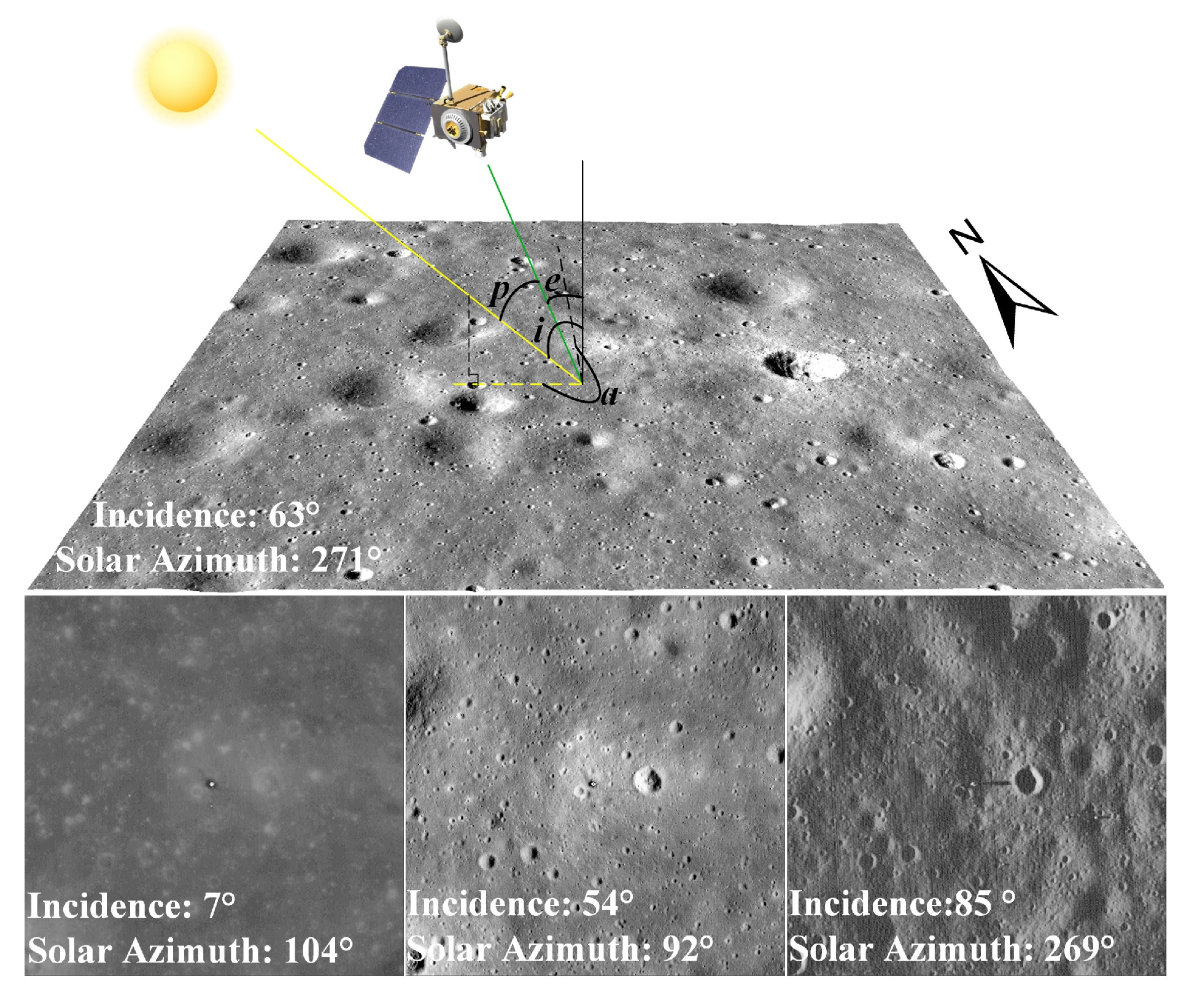
Figure 1.
Schematic of illumination angles and examples of lunar orbiter images captured under different illumination conditions. i.e., p are the solar incidence, emission and phase angles respectively. α is the solar azimuth angle defined as the angle between the direction of sunlight and the north direction on the lunar surface. The image blocks are sourced from Lunar Reconnaissance Orbiter Camera (LROC), which are centered on the Apollo 11 lander. The corresponding image product IDs are M150361817RE, M1134046721RE, M113799518RE, and M1277607697LE, respectively.
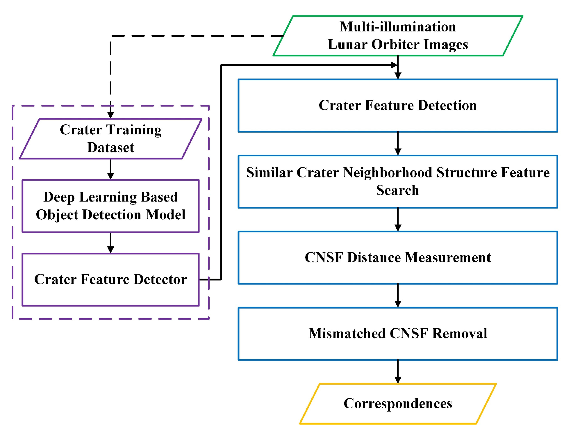
Figure 2.
Framework of the proposed CNSFM method.
Figure 2.
Framework of the proposed CNSFM method.
Figure 3.
Similarity invariants. are the corresponding locations of after similarity transformation . are the diameters of features . Side length represents the distance between points and . Angle represents the angle formed at point in the clockwise direction, from to . Other side lengths and angles follow the same definitions.
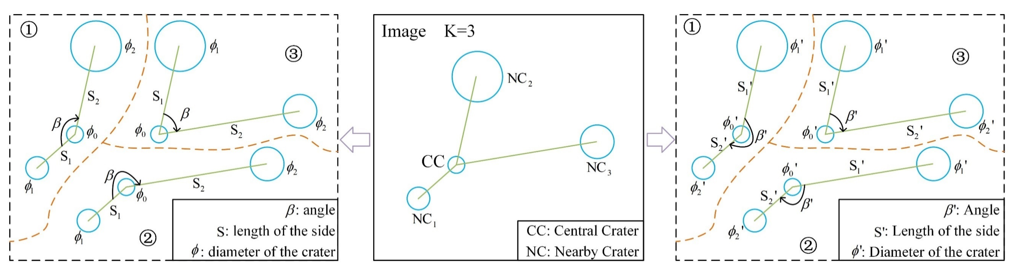
Figure 4.
Angle structures within a CNSF as K = 3. The angle structures on the left are divided with CC-NC1 as the starting edge, while the angle structures on the right are divided with CC-NC2 as the starting edge. The corresponding angles on the left and right of the diagram may be equal or may add up to 360°.
Figure 5.
CNSFs when the K value is set to 10. The craters indicated by the yellow lines have no corresponding features on the other side, whereas those indicated by the green lines exhibit corresponding features on both sides.
Figure 5.
CNSFs when the K value is set to 10. The craters indicated by the yellow lines have no corresponding features on the other side, whereas those indicated by the green lines exhibit corresponding features on both sides.
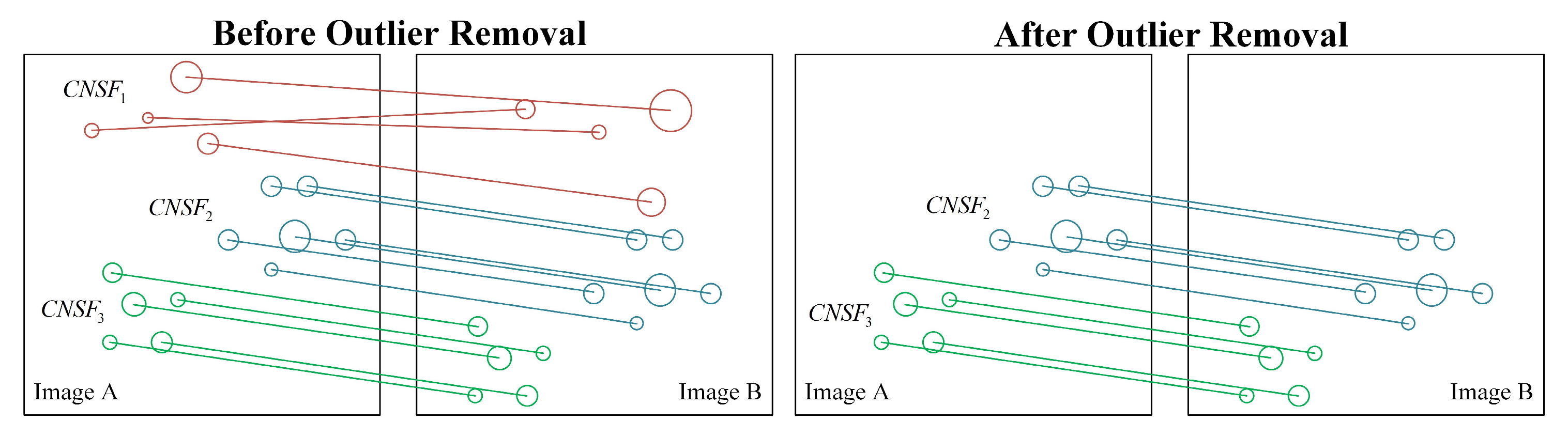
Figure 6.
Outlier removal for CNSFs.
Figure 6.
Outlier removal for CNSFs.
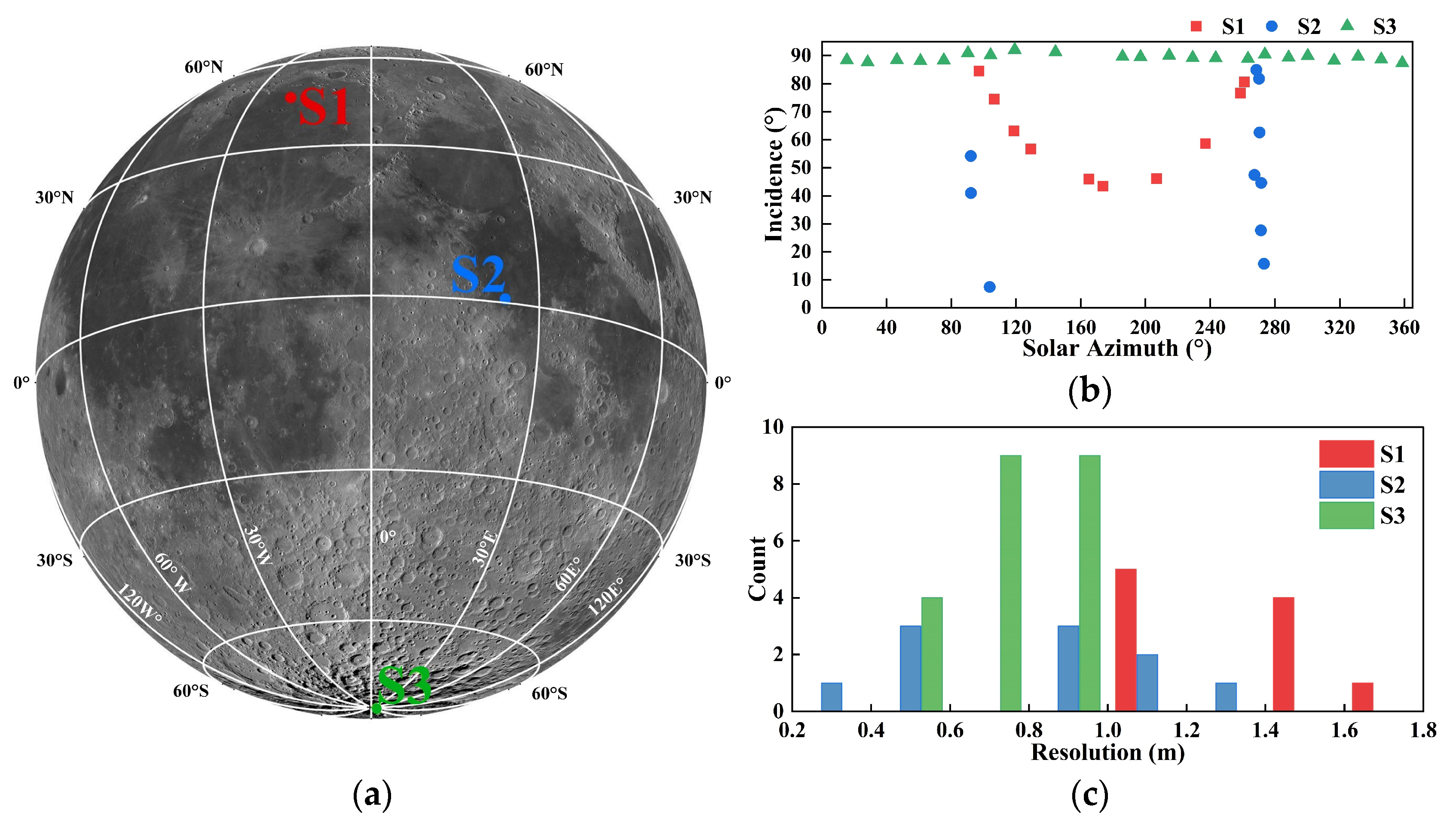
Figure 7.
The spatial distribution of the selected regions in the lunar surface within the evaluation dataset (a). The distribution of the solar azimuth and incidence for all selected images (b). The resolution histogram for all selected images (c).
Figure 7.
The spatial distribution of the selected regions in the lunar surface within the evaluation dataset (a). The distribution of the solar azimuth and incidence for all selected images (b). The resolution histogram for all selected images (c).
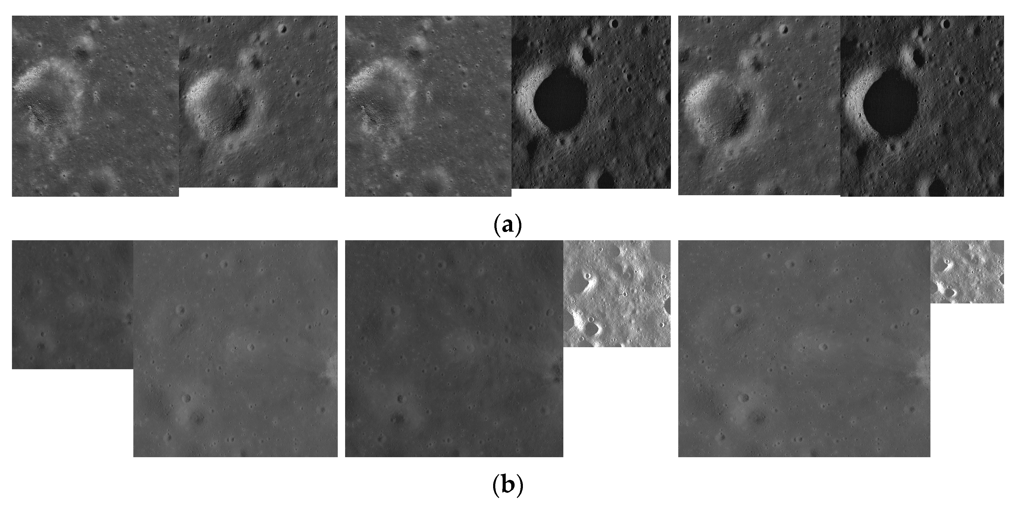
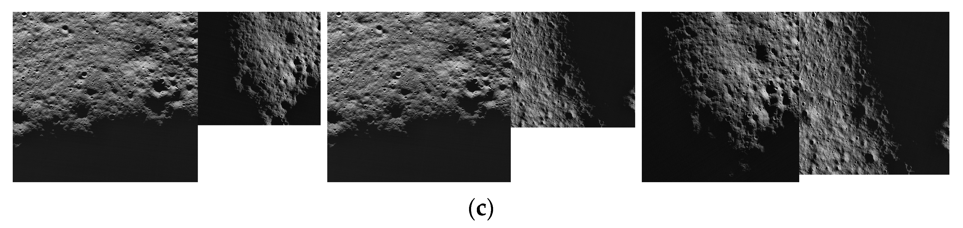
Figure 8.
Sample image pairs of the evaluation dataset. S1 (a), S2 (b), S3 (c).
Figure 8.
Sample image pairs of the evaluation dataset. S1 (a), S2 (b), S3 (c).
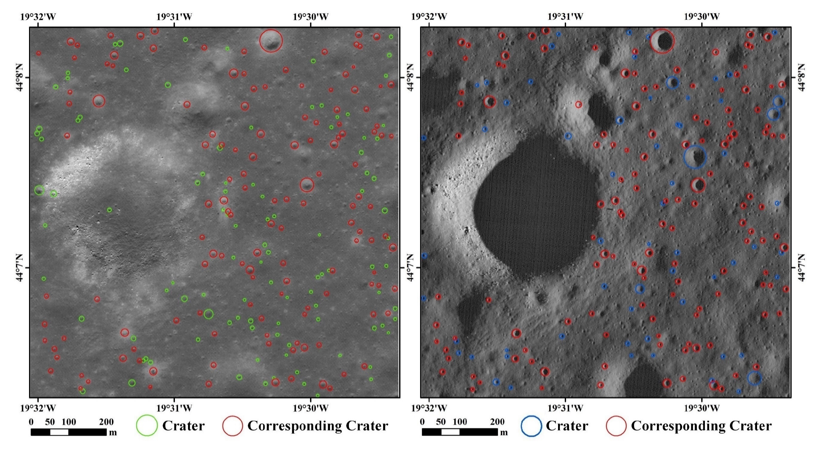
Figure 9.
Crater detection results for a pair of MiLOIs. The image product IDs are M1389516184R and M1276733320L, respectively. The images are centered on the Chang’e 3 lander. Their incidence angles are 43.4° and 84.5°, solar azimuth angles are 173.6° and 97.1°, respectively.
Figure 9.
Crater detection results for a pair of MiLOIs. The image product IDs are M1389516184R and M1276733320L, respectively. The images are centered on the Chang’e 3 lander. Their incidence angles are 43.4° and 84.5°, solar azimuth angles are 173.6° and 97.1°, respectively.
Figure 10.
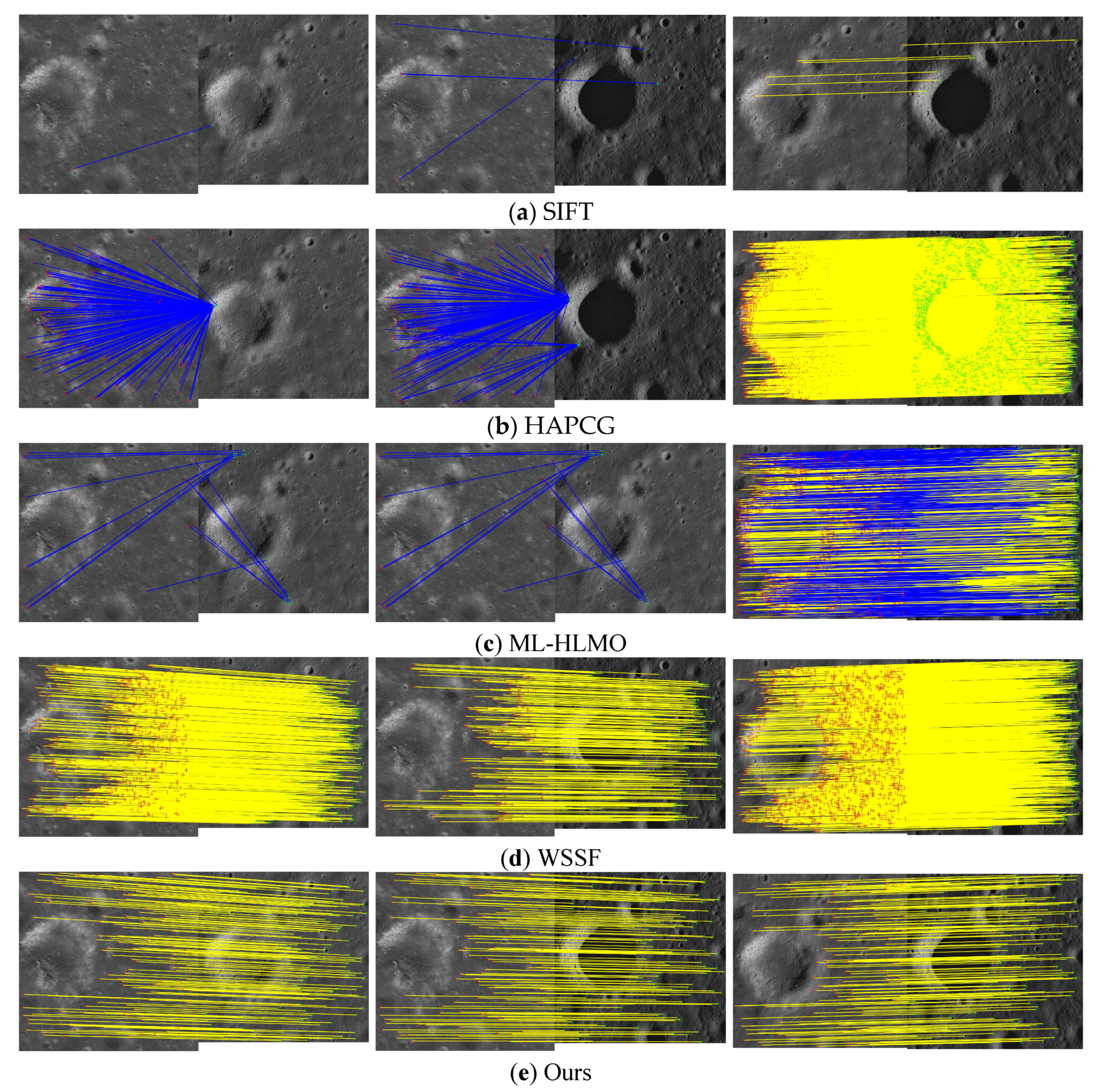
Matching results of sample data from Scene S1. The columns correspond to pairs of images, while rows the correspond to methods. Blue lines indicate incorrect matches, while yellow lines indicate correct matches. SIFT (a), HAPCG (b), ML-HLMO (c), WSSF (d), and CNSFM (e).
Figure 10.
Matching results of sample data from Scene S1. The columns correspond to pairs of images, while rows the correspond to methods. Blue lines indicate incorrect matches, while yellow lines indicate correct matches. SIFT (a), HAPCG (b), ML-HLMO (c), WSSF (d), and CNSFM (e).
Figure 11.
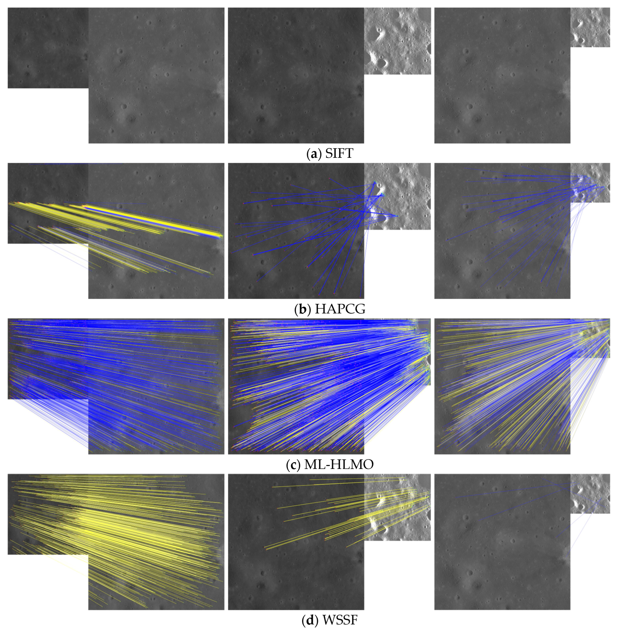
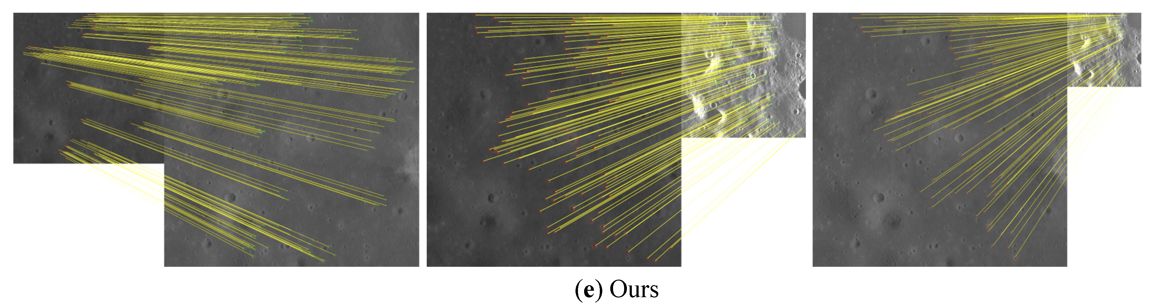
Matching results of sample data from Scene S2. The columns correspond to pairs of images, while rows the correspond to methods. Blue lines indicate incorrect matches, while yellow lines indicate correct matches. SIFT (a), HAPCG (b), ML-HLMO (c), WSSF (d), and CNSFM (e).
Figure 11.
Matching results of sample data from Scene S2. The columns correspond to pairs of images, while rows the correspond to methods. Blue lines indicate incorrect matches, while yellow lines indicate correct matches. SIFT (a), HAPCG (b), ML-HLMO (c), WSSF (d), and CNSFM (e).
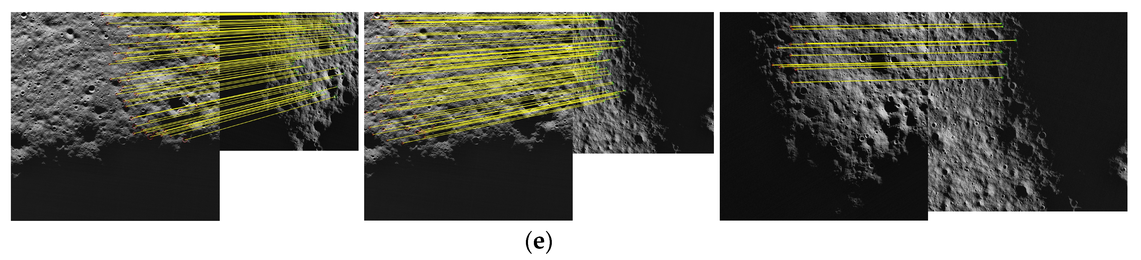
Figure 12.
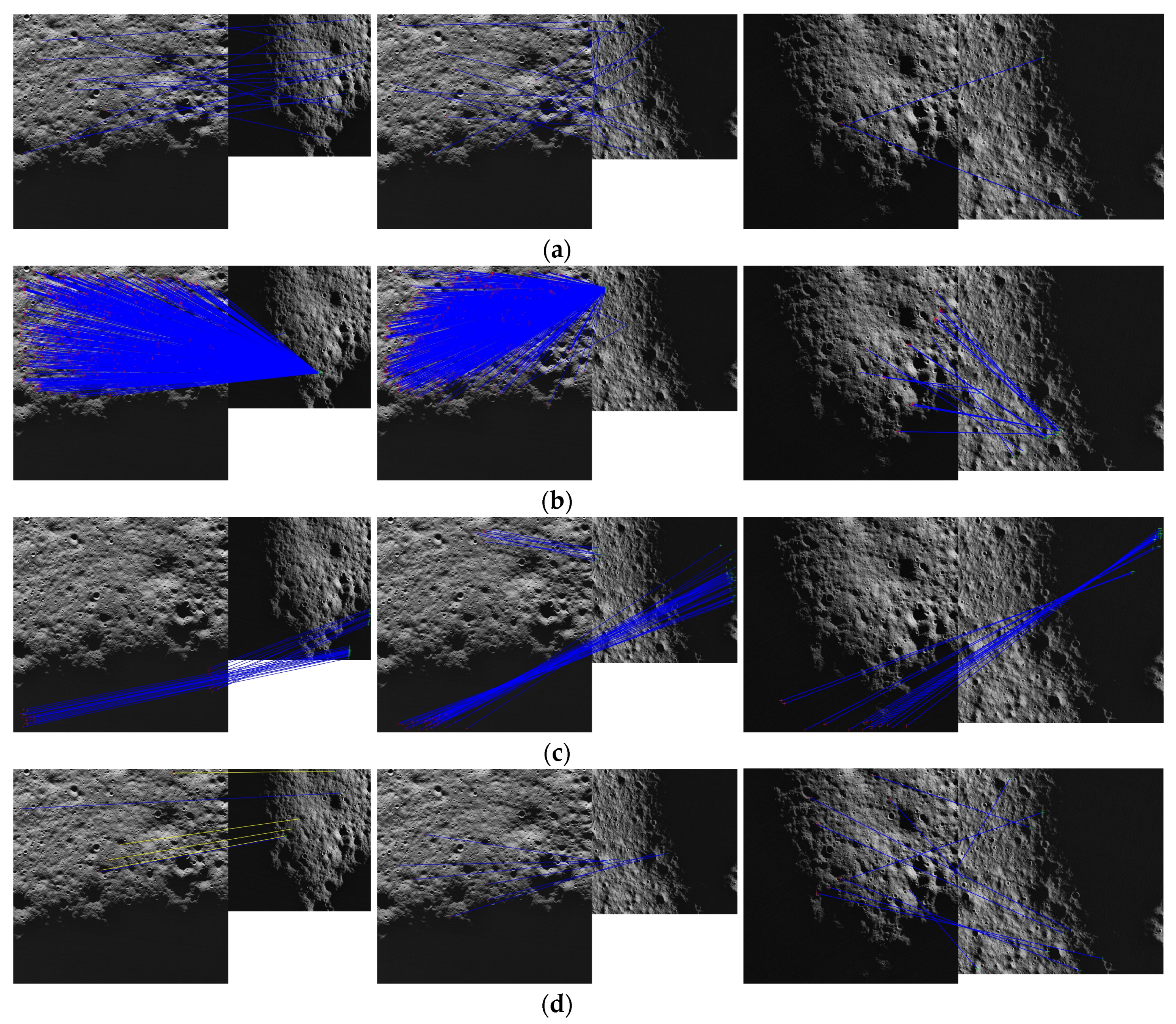
Matching results of sample data from Scene S3. The columns correspond to pairs of images, while rows the correspond to methods. Blue lines indicate incorrect matches, while yellow lines indicate correct matches. SIFT (a), HAPCG (b), ML-HLMO (c), WSSF (d), CNSFM (e).
Figure 12.
Matching results of sample data from Scene S3. The columns correspond to pairs of images, while rows the correspond to methods. Blue lines indicate incorrect matches, while yellow lines indicate correct matches. SIFT (a), HAPCG (b), ML-HLMO (c), WSSF (d), CNSFM (e).
Figure 13.
The frequency distribution of RMSE, with different colors representing different methods.
Figure 13.
The frequency distribution of RMSE, with different colors representing different methods.
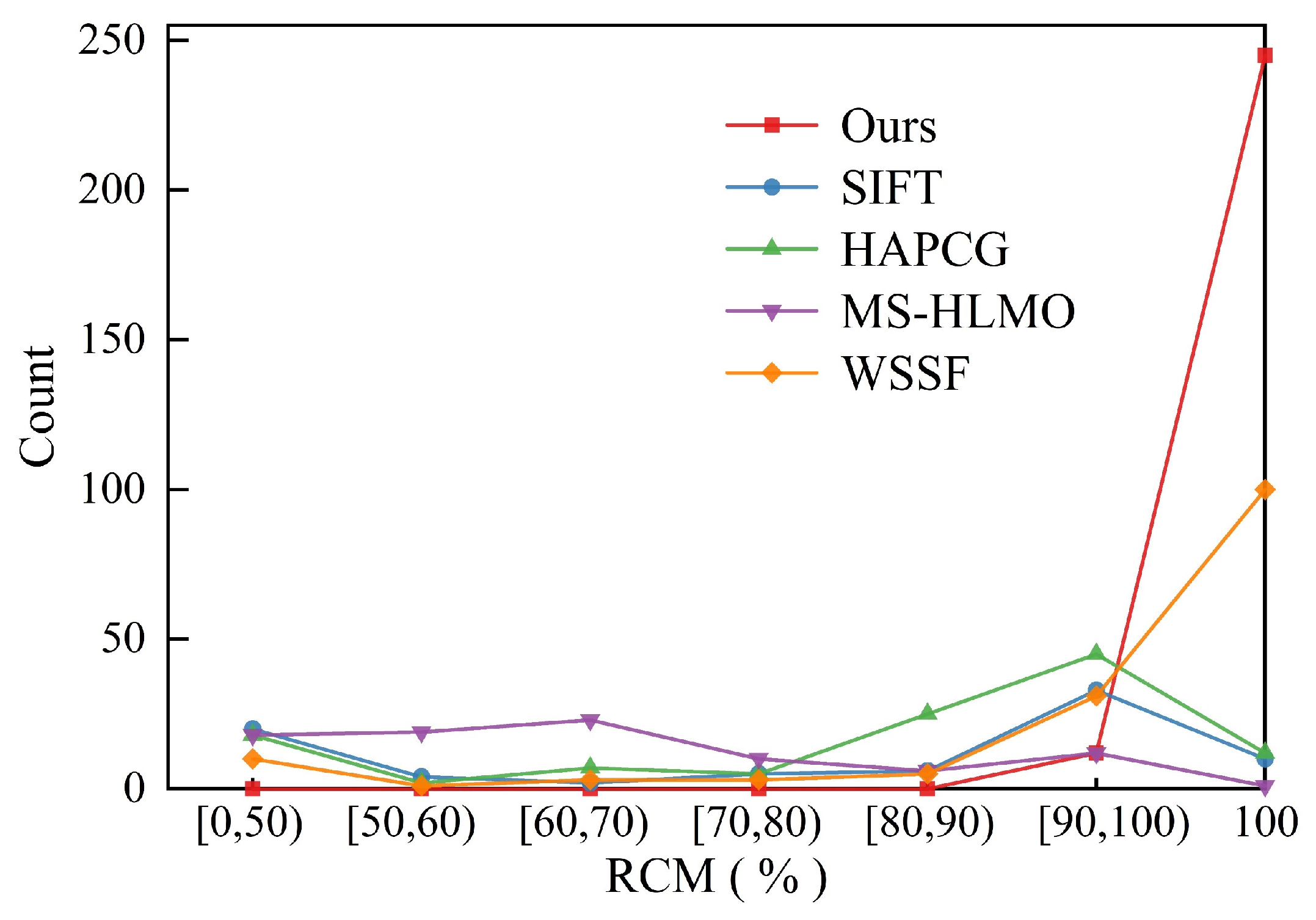
Figure 14.
The frequency distribution of RCM. The horizontal axis represents RCM (in percentage), while the vertical axis represents the number of image pairs within different RCM ranges; different colors correspond to different methods.
Figure 14.
The frequency distribution of RCM. The horizontal axis represents RCM (in percentage), while the vertical axis represents the number of image pairs within different RCM ranges; different colors correspond to different methods.
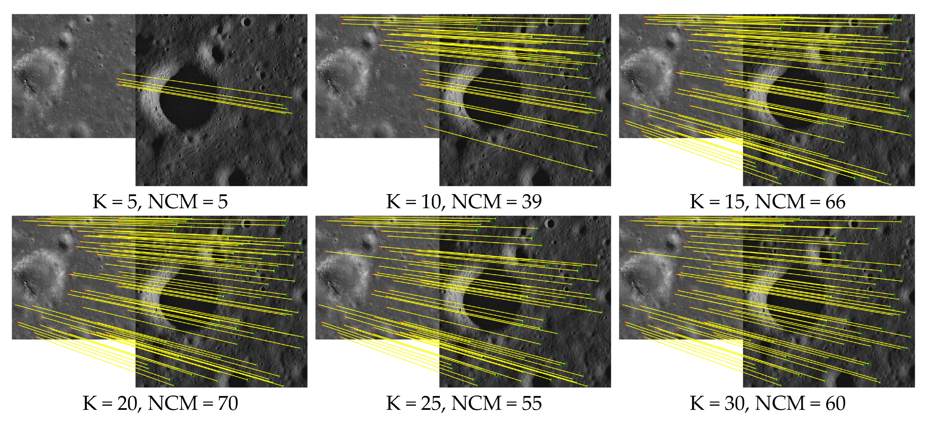
Figure 15.
The matching results of a sample image pair for different K values.
Figure 15.
The matching results of a sample image pair for different K values.
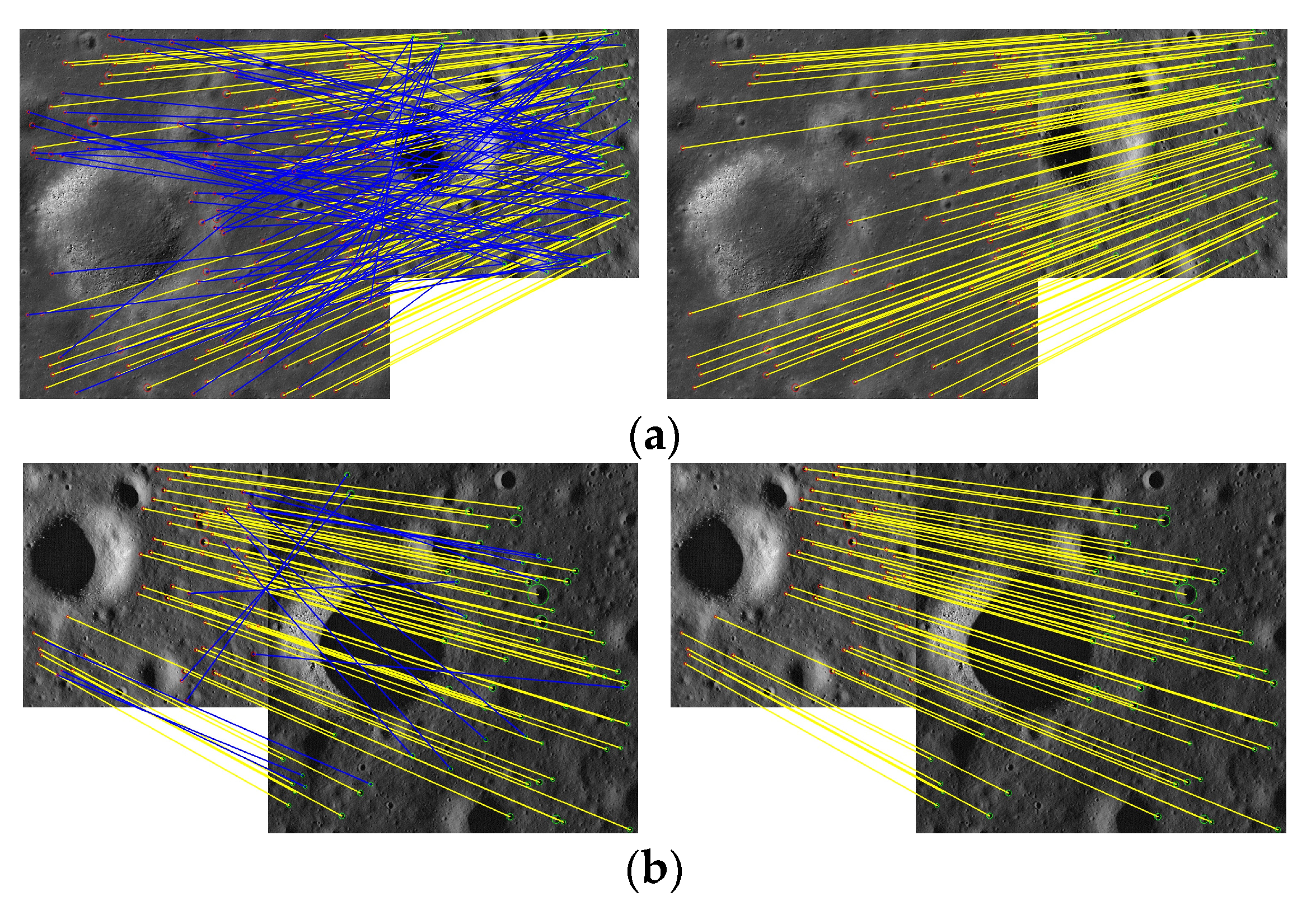
Figure 16.
(a,b) Matching results of two sample image pairs without (left) and with (right) mismatched CNSF removal. Blue lines indicate incorrect matches, while yellow lines indicate correct matches.
Figure 16.
(a,b) Matching results of two sample image pairs without (left) and with (right) mismatched CNSF removal. Blue lines indicate incorrect matches, while yellow lines indicate correct matches.
Figure 17.
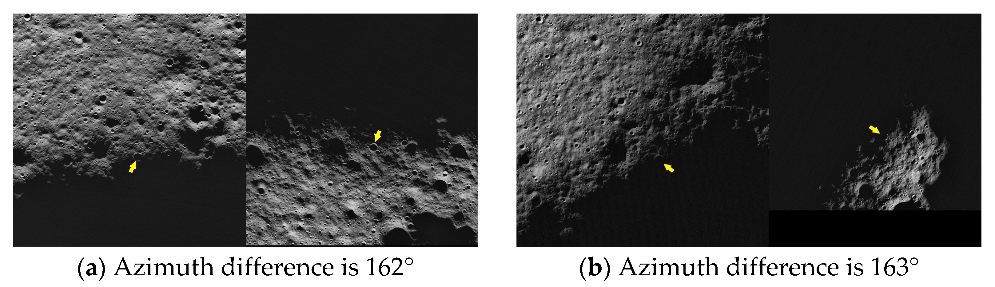
Two image pairs with failed matches in region S3. The yellow arrows point to corresponding impact craters located along the shadow boundaries.
Figure 17.
Two image pairs with failed matches in region S3. The yellow arrows point to corresponding impact craters located along the shadow boundaries.
Figure 18.
The relationship between successful matching and Solar Azimuth differences. Each point represents a successful match, with different colors representing different matching methods.
Figure 18.
The relationship between successful matching and Solar Azimuth differences. Each point represents a successful match, with different colors representing different matching methods.
Table 1.
Comparisons on SR Metric (%).
Table 1.
Comparisons on SR Metric (%).
| Region | SIFT | HAPCG | ML-HLMO | WSSF | Ours |
|---|
| S1 | 33.3 | 66.7 | 33.3 | 100 | 100 |
| S2 | 24.4 | 48.9 | 88.9 | 66.7 | 100 |
| S3 | 17.3 | 22.1 | 13.9 | 31.2 | 72.3 |
Table 2.
The average value of RMSE (pixel).
Table 2.
The average value of RMSE (pixel).
| Region | SIFT | HAPCG | ML-HLMO | WSSF | Ours |
|---|
| S1 | 3.8 | 3.2 | 4.1 | 1.9 | 1.0 |
| S2 | 4.2 | 3.8 | 3.1 | 3.0 | 1.5 |
| S3 | 4.3 | 4.4 | 4.7 | 4.1 | 2.2 |
Table 3.
The average value of RCM (%).
Table 3.
The average value of RCM (%).
| Region | SIFT | HAPCG | ML-HLMO | WSSF | Ours |
|---|
| S1 | 93.3 | 93.8 | 90.7 | 98.8 | 100 |
| S2 | 93.2 | 88.1 | 62.5 | 98.6 | 99.3 |
| S3 | 71.0 | 79.4 | 52.0 | 92.2 | 100 |
Table 4.
The average value of NCM.
Table 4.
The average value of NCM.
| Region | SIFT | HAPCG | ML-HLMO | WSSF | Ours |
|---|
| S1 | 47 | 942 | 930 | 877 | 93 |
| S2 | 65 | 2267 | 1332 | 567 | 150 |
| S3 | 108 | 564 | 112 | 233 | 57 |
Table 5.
Matching results with difference value of parameter K.
Table 5.
Matching results with difference value of parameter K.
| Metric | Values of Parameter K |
|---|
| 5 | 10 | 15 | 20 | 25 | 30 |
|---|
| Average NCM | 25 | 82 | 93 | 93 | 89 | 80 |
| SR (%) | 93.3 | 100 | 100 | 100 | 100 | 100 |
| Average MT(s) | 1.3 | 3.5 | 23.8 | 91.1 | 239.6 | 530.0 |
Table 6.
Results of ablation experiment.
Table 6.
Results of ablation experiment.
| Metric | CNSFM Without MCR | Full CNSFM |
|---|
| Average RCM (%) | 62.2 | 100 |


 ,
, 


