
Synergic Lidar Observations of Ozone Episodes and Transport During 2023 Summer AGES+ Campaign in NYC Region


Abstract

1. Introduction
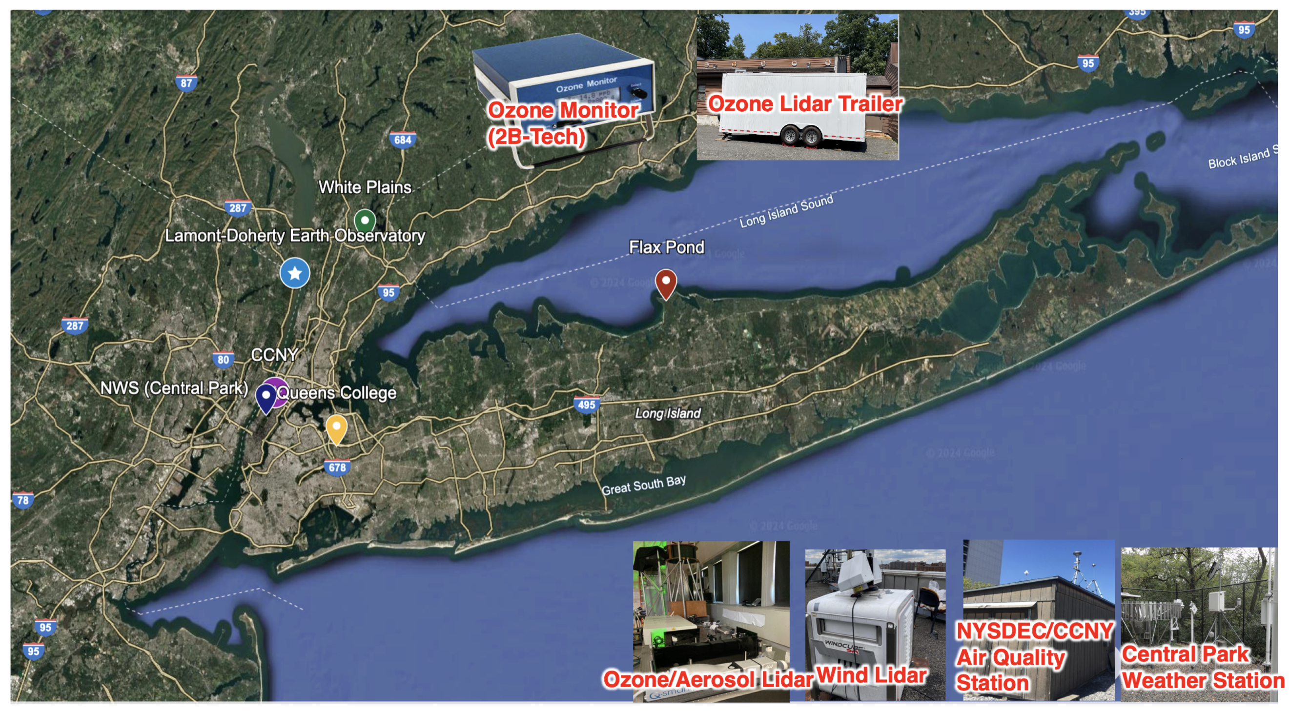
2. Materials and Methods
3. Results
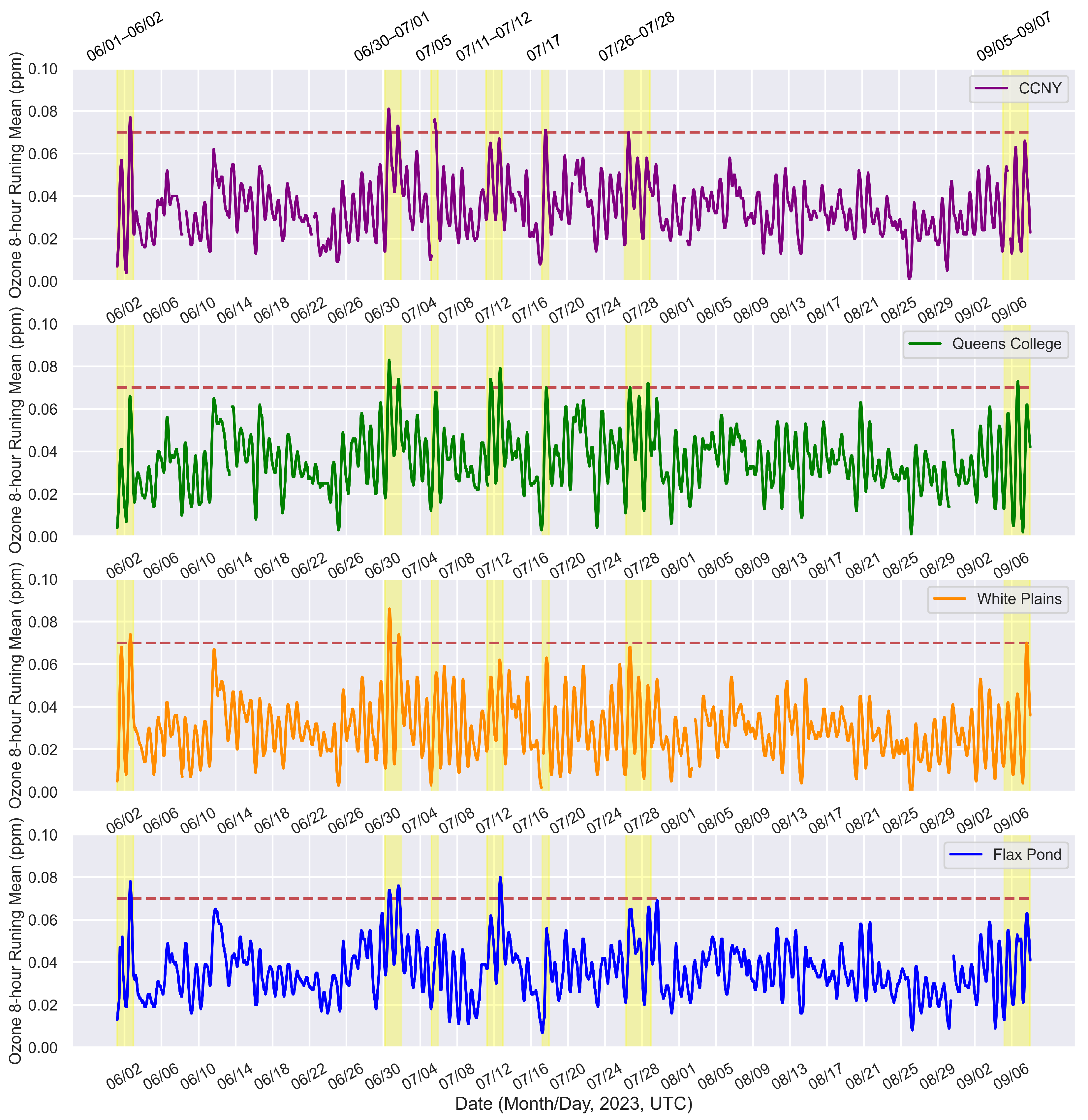
3.1. Overview
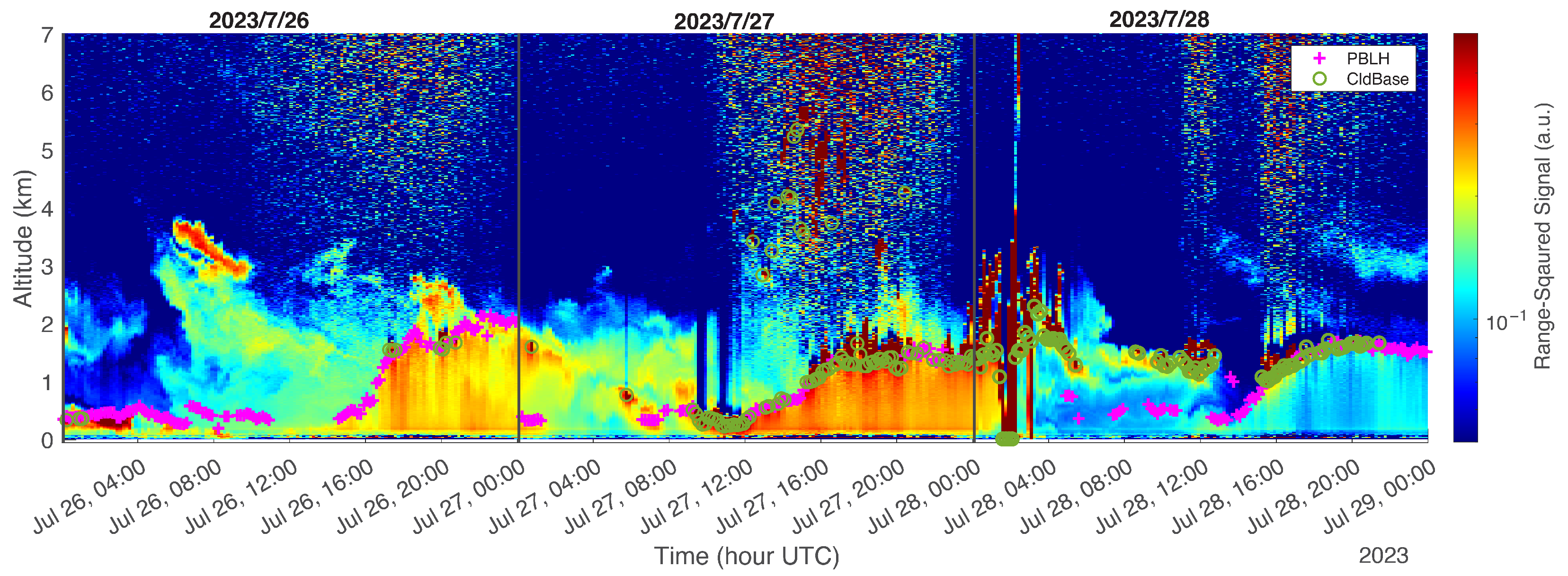
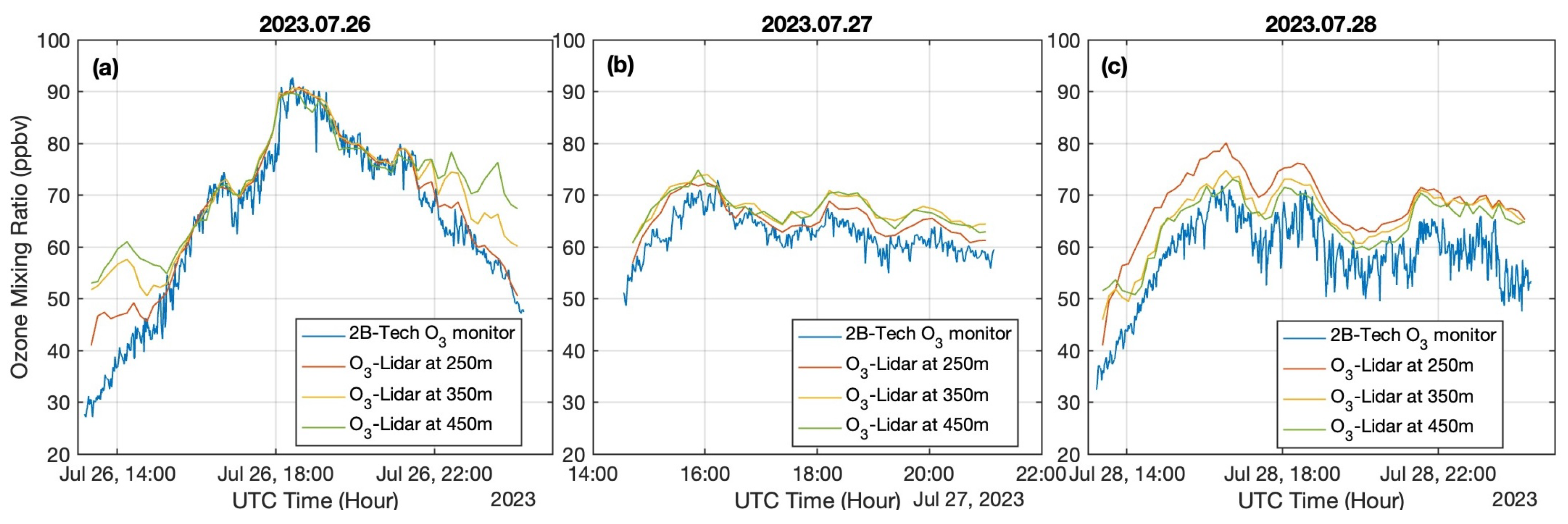
3.2. Case Study 1: Ozone Formation and Aloft Ozone/Aerosol Plume Transport and Mixing into the PBL (26–28 July 2023)
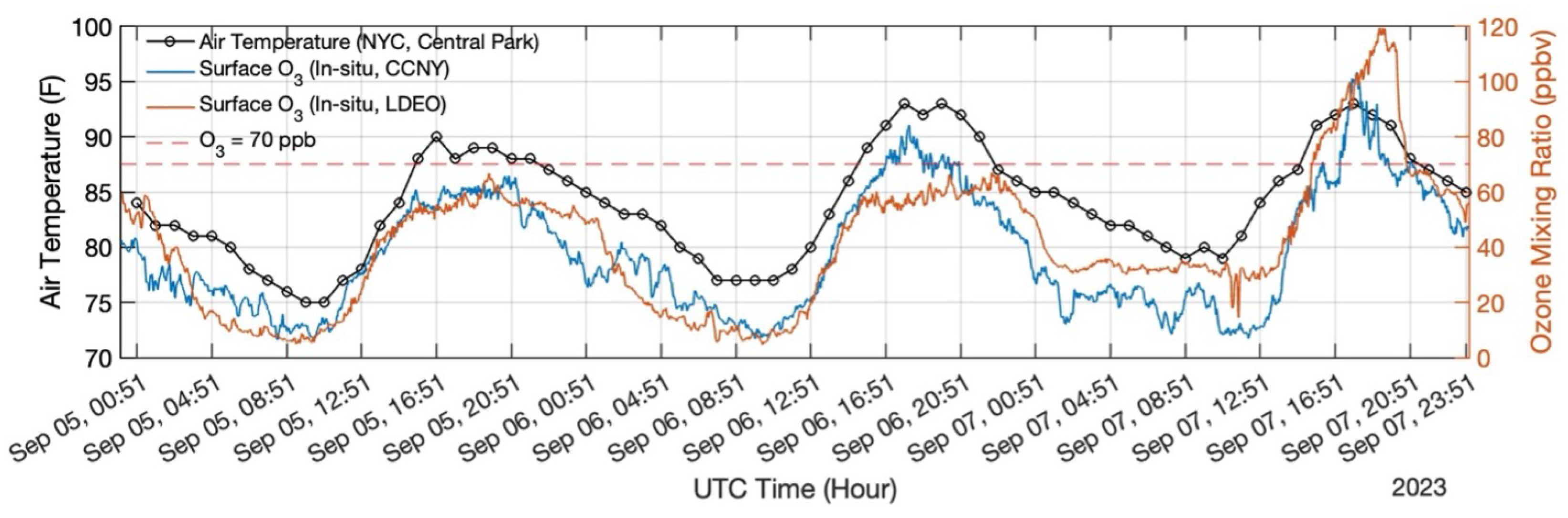
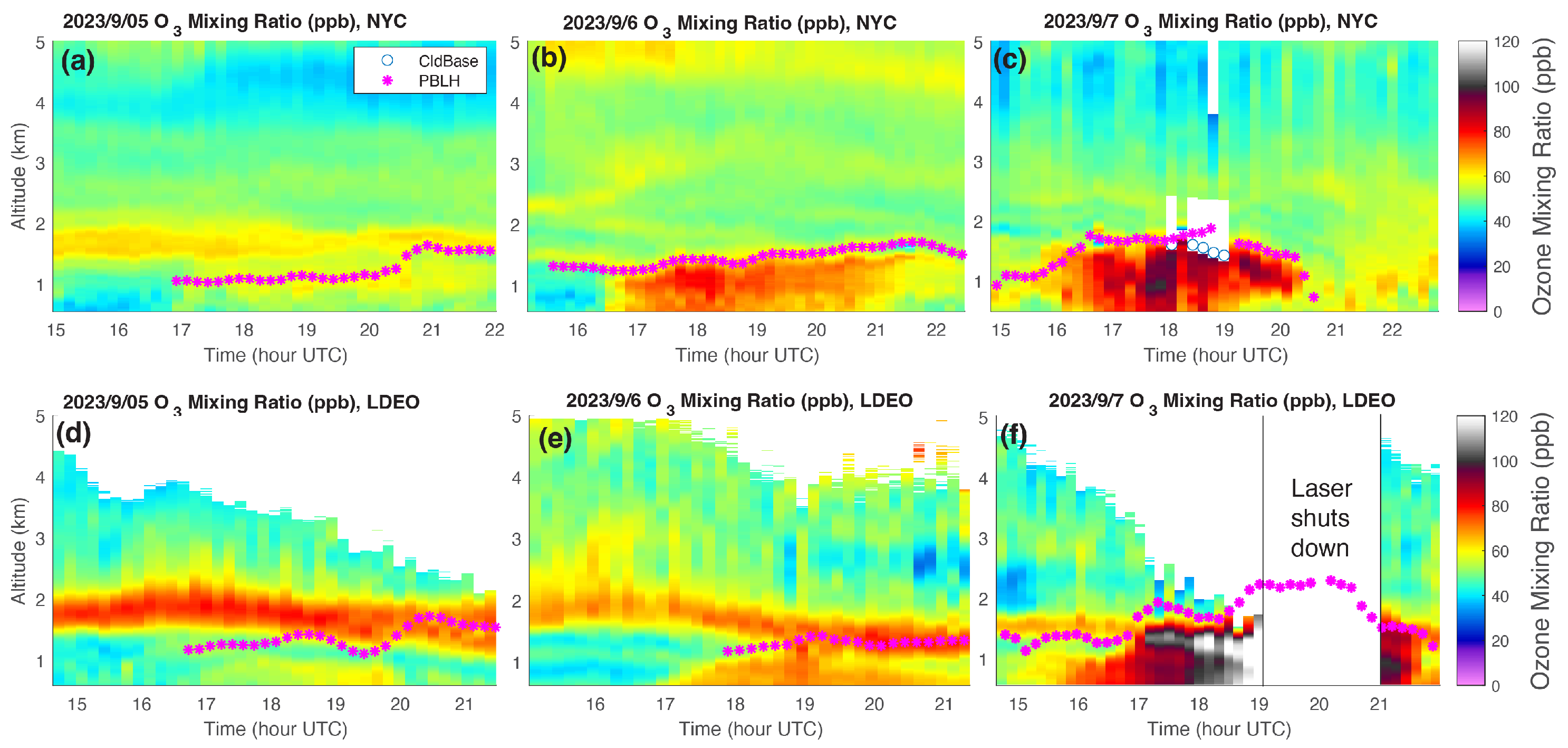
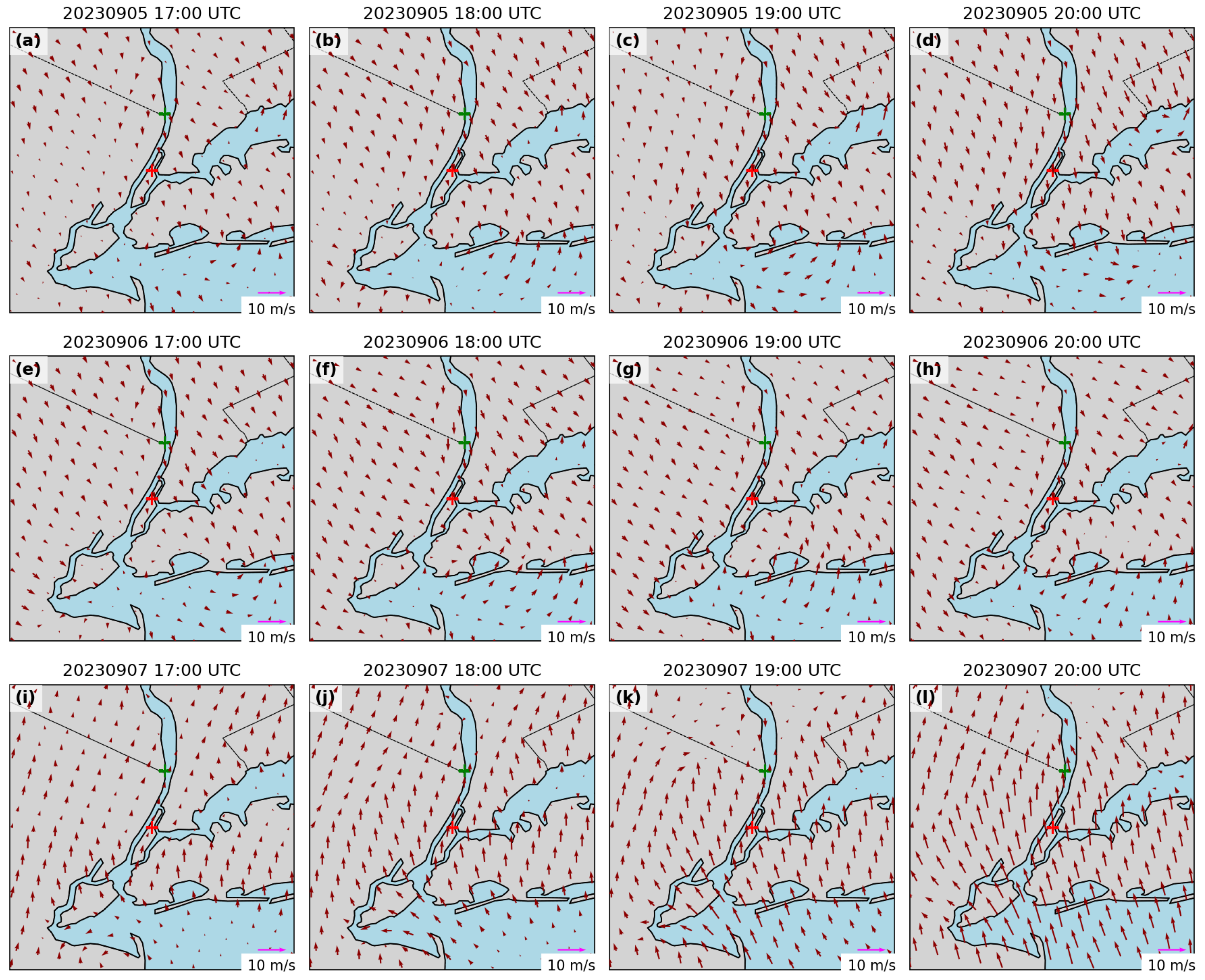
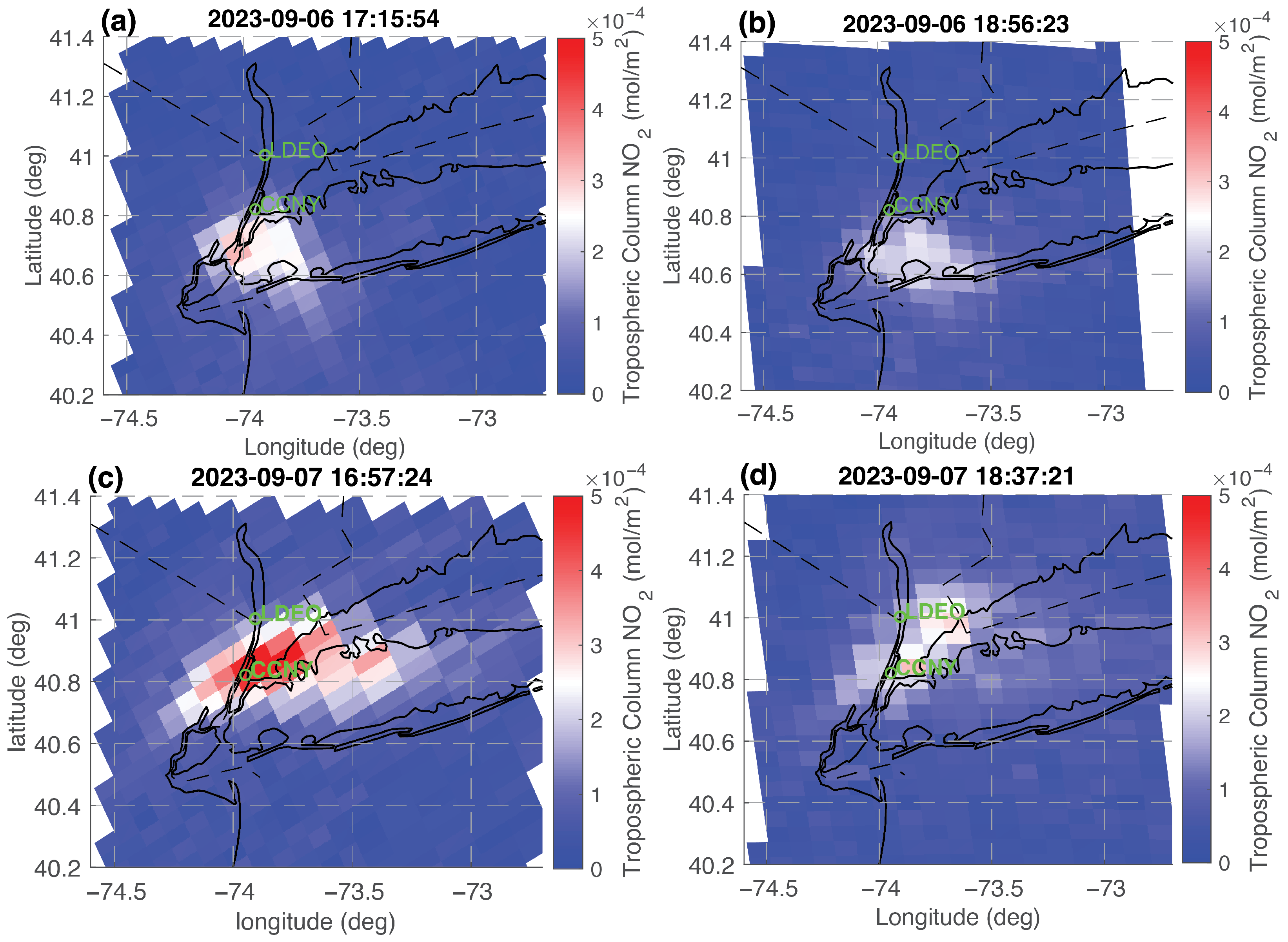
3.3. Case Study 2: Ozone Urban Plume Transport to Downwind Suburban Area (5–7 September 2023)
4. Discussion
5. Conclusions
Author Contributions
Funding
Data Availability Statement
Acknowledgments
Conflicts of Interest
Abbreviations
| DIAL | Differential Absorption Lidar |
| CCNY | City College of New York |
| PBL | Planetary Boundary Layer |
| LDEO | Lamont–Doherty Earth Observatory |
| HRRR | High-Resolution Rapid Refresh |
| TROPOMI | TROPOspheric Monitoring Instrument |
| NOx | Nitrogen Oxide |
| NO2 | Nitrogen Dioxide |
| NO | Nitrogen Monoxide |
| VOC | Volatile Organic Compound |
| CH4 | Methane |
| CO | Carbon Monoxide |
| EPA | Environmental Protection Agency |
| NAAQS | National Ambient Air Quality Standards |
| MDA8O3 | Maximum Daily 8 h Average Ozone Level |
| NYC | New York City |
| NY Metro | New York Metropolitan Area |
| LIS | Long Island Sound |
| NJ | New Jersey |
| PA | Philadelphia |
| AGES+ | AEROMMA+CUPiDS, GOTHAAM, EPCAPE, STAQS, and others |
| AEROMMA | Atmospheric Emissions and Reactions Observed from Megacities to Marine Areas |
| CUPiDS | Coastal Urban Plume Dynamics Study |
| NOAA | National Atmospheric and Oceanic Administration |
| STAQS | Synergistic TEMPO Air Quality Science Mission |
| NASA | National Aeronautics and Space Administration |
| TOLNet | Tropospheric Ozone Lidar Network |
| FWHM | Full Width at Half Maximum |
| PMT | Photomultiplier Tube |
| PBLH | Planetary Boundary Layer Height |
| DBS | Doppler-Beam Swing |
| SNR | Signal-to-Noise Ratio |
| NYSDEC | New York State Department of Environment Conservation |
| AQ | Air Quality |
| UTC | Coordinated Universal Time |
| EDT | Eastern Daylight Time |
References
- Ebi, K.L.; McGregor, G. Climate change, tropospheric ozone and particulate matter, and health impacts. Environ. Health Perspect. 2008, 116, 1449–1455. [Google Scholar] [CrossRef]
- Wang, Y.; Wild, O.; Chen, X.; Wu, Q.; Gao, M.; Chen, H.; Qi, Y.; Wang, Z. Health impacts of long-term ozone exposure in China over 2013–2017. Environ. Int. 2020, 144, 106030. [Google Scholar] [CrossRef]
- Zhang, J.; Wei, Y.; Fang, Z. Ozone pollution: A major health hazard worldwide. Front. Immunol. 2019, 10, 2518. [Google Scholar] [CrossRef]
- Anenberg, S.C.; Horowitz, L.W.; Tong, D.Q.; West, J.J. An estimate of the global burden of anthropogenic ozone and fine particulate matter on premature human mortality using atmospheric modeling. Environ. Health Perspect. 2010, 118, 1189–1195. [Google Scholar] [CrossRef]
- Kleinman, L.I.; Daum, P.H.; Lee, Y.N.; Nunnermacker, L.J.; Springston, S.R.; Weinstein-Lloyd, J.; Rudolph, J. A comparative study of ozone production in five US metropolitan areas. J. Geophys. Res. Atmos. 2005, 110, D02301. [Google Scholar] [CrossRef]
- Martins, D.; Stauffer, R.; Thompson, A.; Knepp, T.; Pippin, M. Surface ozone at a coastal suburban site in 2009 and 2010: Relationships to chemical and meteorological processes. J. Geophys. Res. Atmos. 2012, 117, D05306. [Google Scholar] [CrossRef]
- Zhao, K.; Bao, Y.; Huang, J.; Wu, Y.; Moshary, F.; Arend, M.; Wang, Y.; Lee, X. A high-resolution modeling study of a heat wave-driven ozone exceedance event in New York City and surrounding regions. Atmos. Environ. 2019, 199, 368–379. [Google Scholar] [CrossRef]
- Ma, S.; Tong, D.; Lamsal, L.; Wang, J.; Zhang, X.; Tang, Y.; Saylor, R.; Chai, T.; Lee, P.; Campbell, P.; et al. Improving predictability of high-ozone episodes through dynamic boundary conditions, emission refresh and chemical data assimilation during the Long Island Sound Tropospheric Ozone Study (LISTOS) field campaign. Atmos. Chem. Phys. 2021, 21, 16531–16553. [Google Scholar] [CrossRef]
- Torres-Vazquez, A.; Pleim, J.; Gilliam, R.; Pouliot, G. Performance Evaluation of the Meteorology and Air Quality Conditions From Multiscale WRF-CMAQ Simulations for the Long Island Sound Tropospheric Ozone Study (LISTOS). J. Geophys. Res. Atmos. 2022, 127, e2021JD035890. [Google Scholar] [CrossRef]
- Kleinman, L.I.; Daum, P.H.; Imre, D.G.; Lee, J.H.; Lee, Y.N.; Nunnermacker, L.J.; Springston, S.R.; Weinstein-Lloyd, J.; Newman, L. Ozone production in the New York City urban plume. J. Geophys. Res. Atmos. 2000, 105, 14495–14511. [Google Scholar] [CrossRef]
- Zhang, J.; Mak, J.; Wei, Z.; Cao, C.; Ninneman, M.; Marto, J.; Schwab, J.J. Long Island enhanced aerosol event during 2018 LISTOS: Association with heatwave and marine influences. Environ. Pollut. 2021, 270, 116299. [Google Scholar] [CrossRef]
- Darby, L.S.; McKeen, S.A.; Senff, C.J.; White, A.B.; Banta, R.M.; Post, M.J.; Brewer, W.A.; Marchbanks, R.; Alvarez, R.J.; Peckham, S.E.; et al. Ozone differences between near-coastal and offshore sites in New England: Role of meteorology. J. Geophys. Res. Atmos. 2007, 112, D16S91. [Google Scholar] [CrossRef]
- Solberg, S.; Hov, Ø.; Søvde, A.; Isaksen, I.; Coddeville, P.; De Backer, H.; Forster, C.; Orsolini, Y.; Uhse, K. European surface ozone in the extreme summer 2003. J. Geophys. Res. Atmos. 2008, 113, D07307. [Google Scholar] [CrossRef]
- Masiol, M.; Hopke, P.; Felton, H.; Frank, B.; Rattigan, O.; Wurth, M.; LaDuke, G. Analysis of major air pollutants and submicron particles in New York City and Long Island. Atmos. Environ. 2017, 148, 203–214. [Google Scholar] [CrossRef]
- Tzortziou, M.; Kwong, C.F.; Goldberg, D.; Schiferl, L.; Commane, R.; Abuhassan, N.; Szykman, J.J.; Valin, L.C. Declines and peaks in NO2 pollution during the multiple waves of the COVID-19 pandemic in the New York metropolitan area. Atmos. Chem. Phys. 2022, 22, 2399–2417. [Google Scholar] [CrossRef]
- Rubino, R.; Bruckman, L.; Magyar, J. Ozone transport. J. Air Pollut. Control Assoc. 1976, 26, 972–975. [Google Scholar] [CrossRef]
- Godowitch, J.; Hogrefe, C.; Rao, S. Diagnostic analyses of a regional air quality model: Changes in modeled processes affecting ozone and chemical-transport indicators from NOx point source emission reductions. J. Geophys. Res. Atmos. 2008, 113, D19303. [Google Scholar] [CrossRef]
- Ninneman, M.; Demerjian, K.; Schwab, J. Ozone production efficiencies at rural New York state locations: Relationship to oxides of nitrogen concentrations. J. Geophys. Res. Atmos. 2019, 124, 2363–2376. [Google Scholar] [CrossRef]
- Han, Z.; González-Cruz, J.; Liu, H.; Melecio-Vázquez, D.; Gamarro, H.; Wu, Y.; Moshary, F.; Bornstein, R. Observed sea breeze life cycle in and around NYC: Impacts on UHI and ozone patterns. Urban Clim. 2022, 42, 101109. [Google Scholar] [CrossRef]
- Zhang, J.; Catena, A.; Shrestha, B.; Freedman, J.; McCabe, E.; Schwab, M.J.; Felton, D.; Kent, J.; Gaza, B.; Schwab, J.J. Unraveling the interaction of urban emission plumes and marine breezes involved in the formation of summertime coastal high ozone on Long Island. Environ. Sci. Atmos. 2022, 2, 1438–1449. [Google Scholar] [CrossRef]
- Couillard, M.H.; Schwab, M.J.; Schwab, J.J.; Lu, C.H.; Joseph, E.; Stutsrim, B.; Shrestha, B.; Zhang, J.; Knepp, T.N.; Gronoff, G.P. Vertical profiles of ozone concentrations in the lower troposphere downwind of New York City during LISTOS 2018–2019. J. Geophys. Res. Atmos. 2021, 126, e2021JD035108. [Google Scholar] [CrossRef]
- Nakazato, M.; Nagai, T.; Sakai, T.; Hirose, Y. Tropospheric ozone differential-absorption Lidar using stimulated Raman scattering in carbon dioxide. Appl. Opt. 2007, 46, 2269–2279. [Google Scholar] [CrossRef]
- Strawbridge, K.B.; Travis, M.S.; Firanski, B.J.; Brook, J.R.; Staebler, R.; Leblanc, T. A fully autonomous ozone, aerosol and nighttime water vapor Lidar: A synergistic approach to profiling the atmosphere in the Canadian oil sands region. Atmos. Meas. Tech. 2018, 11, 6735–6759. [Google Scholar] [CrossRef]
- Li, D.; Wu, Y.; Legbandt, T.; Arend, M.; Liang, M.; Moshary, F. Tropospheric Ozone Differential Absorption Lidar (DIAL) Development at New York City. In Proceedings of the International Laser Radar Conference, Virtual, 27 June–1 July 2022; pp. 547–553. [Google Scholar] [CrossRef]
- Li, D. Lidar Remote Sensing of Aerosol and Ozone Profiles and Application to Air Quality Studies in New York City Area. Ph.D. Thesis, The City College of New York, New York, NY, USA, 2023. Available online: https://academicworks.cuny.edu/cc_etds_theses/1145 (accessed on 29 April 2025).
- Sullivan, J.; McGee, T.; Sumnicht, G.; Twigg, L.; Hoff, R. A mobile differential absorption lidar to measure sub-hourly fluctuation of tropospheric ozone profiles in the Baltimore–Washington, DC region. Atmos. Meas. Tech. 2014, 7, 3529–3548. [Google Scholar] [CrossRef]
- Leblanc, T.; Sica, R.J.; Van Gijsel, J.A.; Godin-Beekmann, S.; Haefele, A.; Trickl, T.; Payen, G.; Gabarrot, F. Proposed standardized definitions for vertical resolution and uncertainty in the NDACC lidar ozone and temperature algorithms–Part 1: Vertical resolution. Atmos. Meas. Tech. 2016, 9, 4029–4049. [Google Scholar] [CrossRef]
- Kuang, S.; Burris, J.F.; Newchurch, M.J.; Johnson, S.; Long, S. Differential absorption lidar to measure subhourly variation of tropospheric ozone profiles. IEEE Trans. Geosci. Remote Sens. 2010, 49, 557–571. [Google Scholar] [CrossRef]
- Wu, Y.; Cordero, L.; Gross, B.; Moshary, F.; Ahmed, S. Assessment of CALIPSO attenuated backscatter and aerosol retrievals with a combined ground-based multi-wavelength lidar and sunphotometer measurement. Atmos. Environ. 2014, 84, 44–53. [Google Scholar] [CrossRef]
- Wu, Y.; Nehrir, A.R.; Ren, X.; Dickerson, R.R.; Huang, J.; Stratton, P.R.; Gronoff, G.; Kooi, S.A.; Collins, J.E.; Berkoff, T.A.; et al. Synergistic aircraft and ground observations of transported wildfire smoke and its impact on air quality in New York City during the summer 2018 LISTOS campaign. Sci. Total Environ. 2021, 773, 145030. [Google Scholar] [CrossRef]
- Fernald, F.G. Analysis of atmospheric lidar observations: Some comments. Appl. Opt. 1984, 23, 652–653. [Google Scholar] [CrossRef]
- Li, D.; Wu, Y.; Gross, B.; Moshary, F. Capabilities of an automatic lidar ceilometer to retrieve aerosol characteristics within the planetary boundary layer. Remote Sens. 2021, 13, 3626. [Google Scholar] [CrossRef]
- Ely, T.; Li, D.; Legbandt, T.; Wu, Y.; Arend, M.; Moshary, F. Design of a Mobile Tropospheric Ozone Lidar and Ozone Profiling in New York During Summer 2023. In Proceedings of the 104th AMS Annual Meeting, Baltimore, MD, USA, 28 January–1 February 2024. [Google Scholar]
- Dowell, D.C.; Alexander, C.R.; James, E.P.; Weygandt, S.S.; Benjamin, S.G.; Manikin, G.S.; Blake, B.T.; Brown, J.M.; Olson, J.B.; Hu, M.; et al. The High-Resolution Rapid Refresh (HRRR): An hourly updating convection-allowing forecast model. Part I: Motivation and system description. Weather Forecast. 2022, 37, 1371–1395. [Google Scholar] [CrossRef]
- Blaylock, B.K.; Horel, J.D.; Liston, S.T. Cloud archiving and data mining of High-Resolution Rapid Refresh forecast model output. Comput. Geosci. 2017, 109, 43–50. [Google Scholar] [CrossRef]
- Luo, H.; Lu, C.H. Impacts of local circulations on ozone pollution in the New York metropolitan area: Evidence from three summers of observations. J. Geophys. Res. Atmos. 2024, 129, e2023JD039206. [Google Scholar] [CrossRef]
- Sillman, S. The relation between ozone, NOx and hydrocarbons in urban and polluted rural environments. Atmos. Environ. 1999, 33, 1821–1845. [Google Scholar] [CrossRef]
- Marr, L.C.; Harley, R.A. Spectral analysis of weekday–weekend differences in ambient ozone, nitrogen oxide, and non-methane hydrocarbon time series in California. Atmos. Environ. 2002, 36, 2327–2335. [Google Scholar] [CrossRef]
- Simon, H.; Reff, A.; Wells, B.; Xing, J.; Frank, N. Ozone trends across the United States over a period of decreasing NOx and VOC emissions. Environ. Sci. Technol. 2015, 49, 186–195. [Google Scholar] [CrossRef]
- Li, J.; Wang, Y.; Qu, H. Dependence of summertime surface ozone on NOx and VOC emissions over the United States: Peak time and value. Geophys. Res. Lett. 2019, 46, 3540–3550. [Google Scholar] [CrossRef]
- Wu, Y.; Zhao, K.; Huang, J.; Arend, M.; Gross, B.; Moshary, F. Observation of heat wave effects on the urban air quality and PBL in New York City area. Atmos. Environ. 2019, 218, 117024. [Google Scholar] [CrossRef]
- Singh, S.; Kavouras, I.G. Trends of ground-level ozone in New York city area during 2007–2017. Atmosphere 2022, 13, 114. [Google Scholar] [CrossRef]
- Pan, Y.; Xiang, Y.; Pei, C.; Lv, L.; Chen, Z.; Liu, W.; Zhang, T. Vertical distribution and transport characteristics of ozone pollution based on Lidar observation network and data assimilation over the Pearl River Delta, China. Atmos. Res. 2024, 310, 107643. [Google Scholar] [CrossRef]
- Johnson, M.S.; Rozanov, A.; Weber, M.; Mettig, N.; Sullivan, J.; Newchurch, M.J.; Kuang, S.; Leblanc, T.; Chouza, F.; Berkoff, T.A.; et al. TOLNet validation of satellite ozone profiles in the troposphere: Impact of retrieval wavelengths. Atmos. Meas. Tech. 2024, 17, 2559–2582. [Google Scholar] [CrossRef]
- Johnson, M.S.; Liu, X.; Zoogman, P.; Sullivan, J.; Newchurch, M.J.; Kuang, S.; Leblanc, T.; McGee, T. Evaluation of potential sources of a priori ozone profiles for TEMPO tropospheric ozone retrievals. Atmos. Meas. Tech. 2018, 11, 3457–3477. [Google Scholar] [CrossRef]
- Naeger, A.R.; Newchurch, M.J.; Moore, T.; Chance, K.; Liu, X.; Alexander, S.; Murphy, K.; Wang, B. Revolutionary air-pollution applications from future tropospheric emissions: Monitoring of pollution (TEMPO) observations. Bull. Am. Meteorol. Soc. 2021, 102, E1735–E1741. [Google Scholar] [CrossRef]


Disclaimer/Publisher’s Note: The statements, opinions and data contained in all publications are solely those of the individual author(s) and contributor(s) and not of MDPI and/or the editor(s). MDPI and/or the editor(s) disclaim responsibility for any injury to people or property resulting from any ideas, methods, instructions or products referred to in the content. |
© 2025 by the authors. Licensee MDPI, Basel, Switzerland. This article is an open access article distributed under the terms and conditions of the Creative Commons Attribution (CC BY) license (https://creativecommons.org/licenses/by/4.0/).
Share and Cite
Li, D.; Wu, Y.; Ely, T.; Legbandt, T.; Moshary, F. Synergic Lidar Observations of Ozone Episodes and Transport During 2023 Summer AGES+ Campaign in NYC Region. Remote Sens. 2025, 17, 2303. https://doi.org/10.3390/rs17132303
Li D, Wu Y, Ely T, Legbandt T, Moshary F. Synergic Lidar Observations of Ozone Episodes and Transport During 2023 Summer AGES+ Campaign in NYC Region. Remote Sensing. 2025; 17(13):2303. https://doi.org/10.3390/rs17132303
Chicago/Turabian StyleLi, Dingdong, Yonghua Wu, Thomas Ely, Thomas Legbandt, and Fred Moshary. 2025. "Synergic Lidar Observations of Ozone Episodes and Transport During 2023 Summer AGES+ Campaign in NYC Region" Remote Sensing 17, no. 13: 2303. https://doi.org/10.3390/rs17132303
APA StyleLi, D., Wu, Y., Ely, T., Legbandt, T., & Moshary, F. (2025). Synergic Lidar Observations of Ozone Episodes and Transport During 2023 Summer AGES+ Campaign in NYC Region. Remote Sensing, 17(13), 2303. https://doi.org/10.3390/rs17132303