From Clusters to Communities: Enhancing Wetland Vegetation Mapping Using Unsupervised and Supervised Synergy

Abstract

High thematic resolution vegetation mapping is essential for monitoring wetland ecosystems, supporting conservation, and guiding water management. However, producing accurate, fine-scale vegetation maps in large, heterogeneous floodplain wetlands remains challenging due to complex hydrology, spectral similarity among vegetation types, and the high cost of extensive field surveys. This study addresses these challenges by developing a scalable vegetation classification framework that integrates cluster-guided sample selection, Random Forest modelling, and multi-source remote-sensing data. The approach combines multi-temporal Sentinel-1 SAR, Sentinel-2 optical imagery, and hydro-morphological predictors derived from LiDAR and hydrologically enforced SRTM DEMs. Applied to the Great Cumbung Swamp, a structurally and hydrologically complex terminal wetland in the lower Lachlan River floodplain of Australia, the framework produced vegetation maps at three hierarchical levels: formations (9 classes), functional groups (14 classes), and plant community types (PCTs; 23 classes). The PCT-level classification achieved an overall accuracy of 93.2%, a kappa coefficient of 0.91, and a Matthews correlation coefficient (MCC) of 0.89, with broader classification levels exceeding 95% accuracy. These results demonstrate that, through targeted sample selection and integration of spectral, structural, and terrain-derived data, high-accuracy, high-resolution wetland vegetation mapping is achievable with reduced field data requirements. The hierarchical structure further enables broader vegetation categories to be efficiently derived from detailed PCT outputs, providing a practical, transferable tool for wetland monitoring, habitat assessment, and conservation planning.

1. Introduction

Wetlands, covering approximately 5–10% of Earth’s surface, are among the planet’s most ecologically valuable ecosystems, supporting biodiversity, hydrological regulation, and climate resilience [1,2]. They provide a wide range of ecosystem services, including water purification, carbon sequestration, flood mitigation, and nutrient cycling [3,4]. However, wetlands are increasingly under threat: 30–90% of wetland areas have already been lost or degraded in many parts of the world, primarily due to agricultural conversion, water resource development, urbanization, pollution, and the effects of climate change [2,5]. These pressures are particularly acute in inland wetlands, where flow regulation and land use change can lead to rapid and often irreversible ecological transitions [1,6].

Given these vulnerabilities, the conservation and sustainable management of wetland ecosystems are critical global priorities [7]. Achieving these goals requires timely, accurate, and spatially detailed information on wetland vegetation composition, structure, and dynamics [8]. Vegetation is a key integrator of ecological processes, reflecting both long-term environmental conditions and recent hydrological changes [9]. Therefore, reliable vegetation mapping and monitoring play central roles in wetland conservation efforts—informing restoration planning, evaluating ecosystem responses to water management, and guiding biodiversity assessments [10,11]. However, the complex hydrology and spatial heterogeneity of these wetlands pose persistent challenges for vegetation monitoring, especially across remote inland floodplain systems.

Recent advances in remote sensing and ecological modeling have substantially improved the potential of large-scale wetland vegetation mapping [12]. A number of technological and methodological developments are enabling more accurate and thematically detailed classifications. These developments can be broadly grouped into four key areas. First, the emergence of high-resolution satellite platforms such as Sentinel-2, PlanetScope, and Landsat 8 has enhanced the spectral, spatial, and temporal resolutions available for ecological applications [13]. For example, Sentinel-2 offers 10 m resolution with a 2–5-day revisit frequency and includes red-edge and shortwave infrared bands that are particularly sensitive to vegetation properties (https://s2.pages.eopf.copernicus.eu/pdfs-adfs/MSI/, accessed on 25 May 2025). PlanetScope imagery provides near-daily coverage at 3.1 m resolution, enabling detailed monitoring of phenological patterns [14]. The integration of optical data with Synthetic Aperture Radar (SAR) from sensors like Sentinel-1 and ALOS-2, and with structural information from LiDAR, has further improved the classification of complex wetland environments by capturing vegetation height, moisture status, and subcanopy structure [15,16].

Second, the use of time-series analysis has allowed researchers to track vegetation dynamics over seasonal and interannual cycles. Phenological modeling using harmonic functions or curve fitting on vegetation indices such as NDVI and EVI helps distinguish vegetation types that appear similar in static imagery but differ in growth timing or seasonal behavior [17,18].

Third, advanced machine learning algorithms, particularly Random Forest (RF), Support Vector Machines (SVM), and ensemble methods like Bagged Trees and deep learning models, have become widely used in wetland classification [19]. These approaches handle complex, nonlinear relationships and are resilient to noise and imbalanced training data [20]. Many recent studies report classification accuracies above 85–95% when using such methods across wide ranges of wetland systems [15,16].

Finally, there has been a shift toward higher thematic resolution in classification outputs. Rather than mapping wetlands by broad land-cover categories, many recent studies have focused on identifying individual vegetation communities or functional groups. For example, Lane et al. [21] mapped 22 plant communities in the Selenga River Delta using WorldView-2 and NDVI-based texture features, achieving an accuracy of 86.5%. Similarly, Bhatnagar et al. [18] mapped 18 wetland vegetation types in Irish peatlands using Sentinel-2 and Bagged Tree classifiers, with accuracies reaching up to 87%. These studies illustrate the growing feasibility—but also the complexity—of multi-class wetland vegetation mapping.

Alongside these technological advances, cluster-guided and semi-supervised sampling strategies have been increasingly applied to improve data efficiency and model performance in ecological remote sensing. Cluster-guided approaches, such as K-means clustering [22], group similar observations based on spectral or environmental characteristics, enabling targeted, representative sample selection across heterogeneous landscapes [23]. Semi-supervised methods combine small amounts of labeled data with larger pools of unlabeled data to reduce field sampling effort while capturing complex ecological patterns [24,25]. Together, these approaches offer practical solutions for improving vegetation classification and biodiversity assessment, particularly in remote or data-limited regions [26,27].

These technological advances have collectively enabled more detailed, accurate, and scalable vegetation mapping, particularly in challenging environments like large, heterogeneous floodplain wetlands. However, key challenges persist, including within-class spectral similarity, data scarcity for model training, and difficulties in mapping spectrally mixed or hydrologically dynamic systems [26,28]. The Great Cumbung Swamp, a vast terminal wetland in the lower Lachlan River floodplain, Australia, exemplifies these challenges [28] and serves as the focal site for this study.

Building on these advances, this study integrates multi-source remote-sensing data (Sentinel-1, Sentinel-2, and hydro-morphological variables), time-series information, and a machine learning framework incorporating unsupervised clustering for targeted sample selection. This approach directly addresses the remaining limitations in training data availability, classification complexity, and mapping performance for floodplain wetlands.

The specific objectives of the study were to (1) develop and evaluate a classification framework for inland floodplain wetlands using multi-temporal Sentinel-1 and Sentinel-2 imagery combined with hydro-morphological predictors derived from high-resolution LiDAR and SRTM DEMs; (2) compare model performance across three classification levels—vegetation formation (9), functional group (14), and detailed plant community type (PCT) (23)—to assess the framework’s applicability in fine-resolution vegetation mapping in heterogeneous wetland environments; (3) test the relative contributions of different predictor sets, including (a) Sentinel-1 and Sentinel-2 only, (b) Sentinel-1 only, and (c) hydro-morphological variables alone, and determine whether the integration of spectral, structural, and terrain-derived features improves classification accuracy; and (4) demonstrate the effectiveness of unsupervised clustering in identifying ecologically meaningful training samples, thereby reducing the reliance on field-based data collection and improving the efficiency and scalability of vegetation mapping in remote or data-scarce wetland systems.

The high-resolution vegetation maps generated through this study offer critical benefits for wetland conservation and land management [9]. By providing spatially explicit information on vegetation composition, distribution, and structural diversity, these maps can support restoration planning, inform environmental water allocations, track ecological responses to hydrological interventions, and contribute to long-term monitoring programs across inland wetland landscapes.

2. Materials and Methods

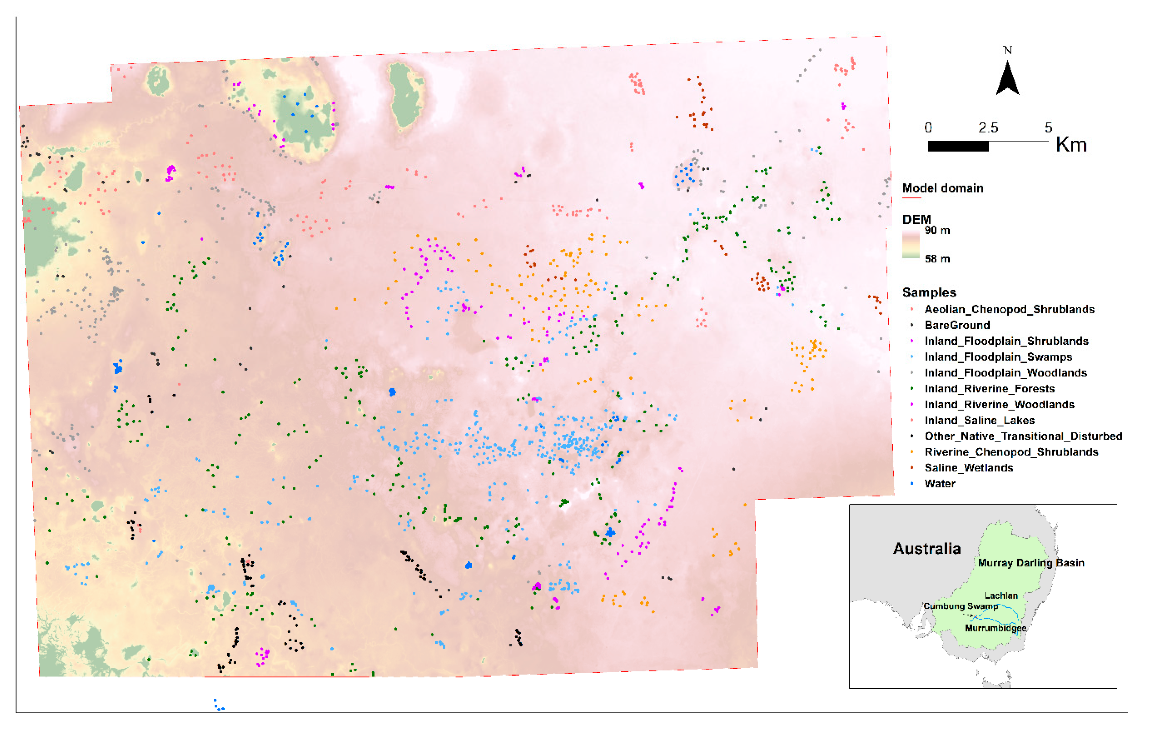
2.1. Study Site

The Great Cumbung Swamp (Figure 1) is a large terminal wetland situated at the lower end of the Lachlan River floodplain in New South Wales, Australia. It spans approximately 14,000 hectares under dry conditions and can expand to 15,000–20,000 hectares during major flooding. The wetland is hydrologically dynamic, influenced by both regulated and unregulated flows, and plays a key role in regional flood attenuation and water quality regulation [28,29] However, the Great Cumbung Swamp is vulnerable to a range of modern environmental pressures, with altered hydrology from water resource development being the most significant [29,30]. Extensive water extraction and river regulation along the Lachlan River have reduced the frequency, extent, and duration of natural flood events, directly affecting the composition and distribution of flood-dependent vegetation communities within the swamp. These hydrological modifications contribute to the decline of critical wetland habitats, underscoring the need for accurate, high-resolution vegetation mapping to support targeted management and restoration efforts.

Recognized for its high conservation value, the Great Cumbung supports a diverse mosaic of habitats, including sedge swamps, reed beds, mixed marshes, and riparian forests. These environments provide critical refuge for a wide range of wetland-dependent fauna, including several threatened species. Conservation efforts emphasize maintaining natural hydrological regimes and protecting the site’s rich vegetation assemblages from degradation [23].

The vegetation of the Lachlan wetlands is highly heterogeneous. Mixed marshes consist of a range of aquatic herbs and grasses that form diverse transitional habitats. Extensive reed beds dominated by Phragmites australis offer structurally complex environments important for waterbird habitat. Zones dominated by Typha spp. are also common and often interspersed within the broader marshland. River red gum (Eucalyptus camaldulensis) forests are primarily found in riparian zones, where they respond strongly to flood pulses. In contrast, black box (E. largiflorens) woodlands occupy higher, less frequently inundated areas of the floodplain, adding further to the structural and compositional diversity of the vegetation mosaic.

Mapping these vegetation communities presents considerable challenges. The close spatial intermingling of plant communities—particularly among marshes, reed beds, Typha-dominated zones, and floodplain woodlands—makes it difficult to delineate clear ecological boundaries. Moreover, the swamp undergoes significant seasonal and interannual variability in water availability, leading to dynamic shifts in vegetation structure and composition. These changes complicate vegetation mapping based on static or single-date imagery. The challenge is further compounded by the presence of spectrally active grassy understory vegetation within forested areas, particularly under river red gum and black box canopies. These understory components often dominate the spectral signals in satellite imagery, confounding efforts to distinguish between overstorey vegetation types and ground layer species while using moderate-resolution sensors. While remote-sensing tools offer broad spatial coverage, they often fall short in capturing the vertical complexity and fine-scale heterogeneity of such mixed vegetation systems [10,31].

To develop a classification framework for detailed vegetation mapping in the Great Cumbung Swamp, we integrated multi-source remote-sensing data with advanced machine learning techniques. We combined Sentinel-2 optical imagery, Sentinel-1 radar data, and hydro-morphological predictors from LiDAR and SRTM DEMs to capture vegetation structure and moisture regimes. An unsupervised clustering approach was used to create an efficient training dataset, enhancing the model’s ability to distinguish between similar vegetation types.

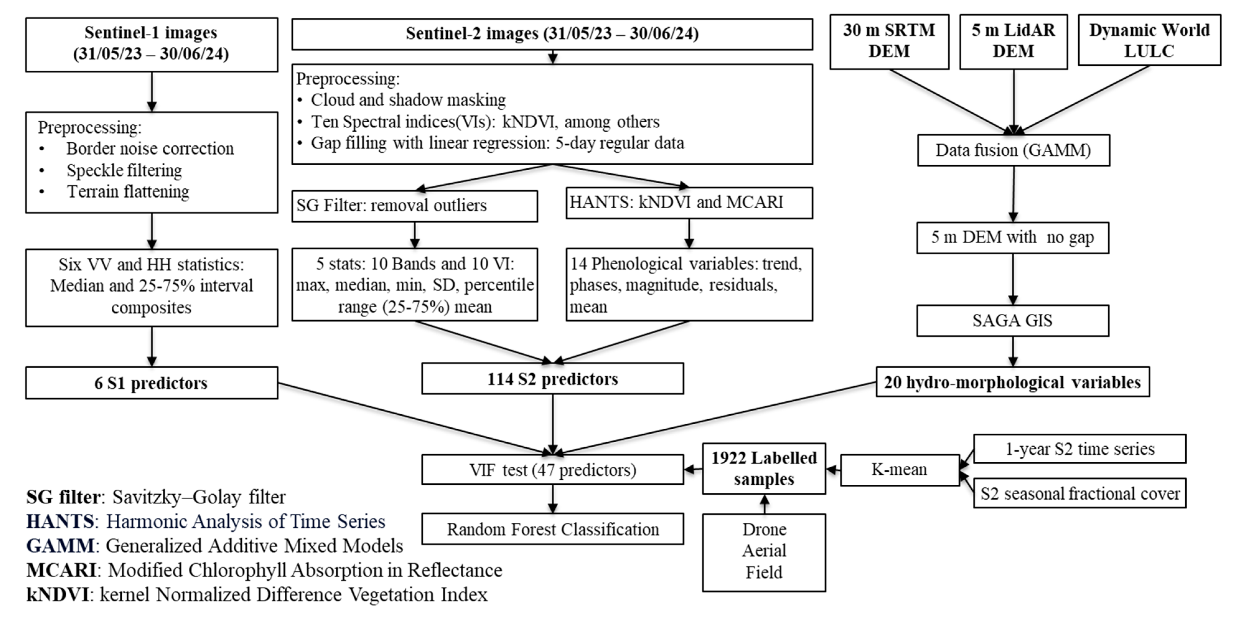
2.2. Data Source and Processing

The classification framework developed in this study integrated multi-source remote-sensing data with terrain-derived variables to produce high-resolution vegetation maps for the Great Cumbung Swamp. Data preprocessing, feature extraction, and modelling were carried out within the Google Earth Engine platform and R statistical environment, allowing for scalable processing of multi-temporal satellite data and extensive predictor variable generation (Figure 2).

2.2.1. Satellite Image Preparation

Sentinel-1 and Sentinel-2 imagery formed the primary satellite data sources. Sentinel-1 C-band SAR data were processed to derive backscatter coefficients (VV and VH), while Sentinel-2 optical imagery was atmospherically corrected using the Surface Reflectance product. To reduce noise and enhance the interpretability of temporal signals, time series from Sentinel-2 were smoothed using the Savitzky–Golay filter [32] and further analyzed using the Harmonic Analysis of Time Series (HANTS) method [33]. This approach allowed for the extraction of seasonal trends, phenological metrics, and vegetation index dynamics across the annual cycle.

Vegetation indices (Supplementary Material S1) were calculated using the Awesome Spectral Indices for Google Earth Engine [34], which includes over 150 indices tailored to vegetation physiology and structure. Nine indices such as the Modified Chlorophyll Absorption in Reflectance Index (MCARI), kernel NDVI (kNDVI), and red-edge-based indices were selected for their ability to capture subtle differences in canopy structure and health. These spectral features were generated for all available Sentinel-2 scenes within the target time period, allowing for the derivation of both static and temporally aggregated variables.

2.2.2. Hydro-Morphological Data

The 5 m LiDAR-derived DEM (digital elevation model) was obtained from Geoscience Australia [35] (https://elevation.fsdf.org.au/) on 15 January 2025. As there are parts of the Great Cumbung Swamp that are not covered by the LiDAR DEM, the LiDAR DEM model was specifically processed in order to eliminate gaps and ensure hydrological consistency. We used the generalized additive mix model (GAMM [36]) to fuse the 5 m LiDAR DEM and the 1 s hydrologically enforced digital elevation model (DEM-H) derived from the SRTM data [37]. In the GAMM, the Dynamic World land cover [38] was used as a random term to account for the effect of land cover on the relationship between LiDAR and DEM-H. The GAMM was implemented using the “mgcv” [39] and “caret” [40] packages in R version 4.3.2 [41], with repeated 20-fold cross-validation (five repeats) to ensure robust model performance. The final model achieved a high R² of 0.89, indicating strong agreement between predicted and actual LiDAR elevations.

With the gap-filled 5 m DEM, 20 hydro-morphological predictors (Supplementary Material S2) were calculated using SAGA GIS (Version: 7.8.2), including relative elevation, plan and profile curvature, terrain ruggedness, slope, and flow accumulation metrics. These variables were designed to capture fine-scale microtopographic variation and hydrological flow pathways that influence wetland vegetation zonation.

2.2.3. Unsupervised Clustering and Training Data Generation

To efficiently generate a high-quality training dataset without extensive field surveys, we adopted a semi-automated approach guided by unsupervised clustering. K-means clustering [22] was applied to a time series of Sentinel-2 spectral indices (NDVI, NDWI, NDMI, and NDRE) and the texture metrics derived from 3 × 3 GLCM NDVI entropy layers, spanning August 2022 to July 2023. Monthly composites (median, standard deviation, and range) were generated in Google Earth Engine from Level-2A surface reflectance images filtered for <30% cloud cover.

A stratified sample of 8000 pixels was used to train a Weka K-means model (K = 30), informed by expert knowledge of vegetation diversity in the region. The clustering captured spectral–temporal variation associated with different vegetation types. Each resulting cluster was manually reviewed by an expert vegetation ecologist, integrating topographic context, high-resolution aerial and drone imagery, and existing ground data to assign clusters to specific plant community types (PCTs) when appropriate. Clusters were retained as training candidates only if they consistently exhibited all of the following:

1.

Visually dominant and identifiable canopy or ground cover species,

2.

Structural characteristics matching known vegetation types,

3.

A landscape position consistent with the ecological descriptions of those types.

Clusters that failed to meet these criteria or represented intra-type variability were either merged or discarded. From verified clusters, random training points were generated and subjected to a secondary expert review to ensure ecological representativeness and spatial precision. Points located near ecotones, boundaries, or anomalies were combined or removed.

This process resulted in a robust, ecologically meaningful training dataset with a total of 1922 samples, enabling the classification of 19 wetland PCTs and 4 other land-cover types (

Table 1. The three vegetation classification themes tested in this study. The inundation gradient decreases within each vegetation formation.

Map ID	Formation	Map ID	Functional Group	Map ID	Plant Community Type	No of Samples
1	Riverine Forest	1	Riverine Forest	1	River Red Gum—sedge open forest	120
		2	Riverine Forest/Woodland	2	River Red Gum—Lignum open forest/woodland	80
2	Riverine Woodland	3	Riverine Woodland	3	River Red Gum—Black Box woodland	145
		3	Floodplain Woodland	4	Black Box—Lignum woodland	90
				5	Black Box—chenopod open woodland	103
				6	Black Box grassy open woodland	52
3	Grassy Wetland	5	(Semi-)permanent Shallow Water	7	(Semi-) permanent freshwater lake	71
		6	Grassy Wetland	8	Tall reedland	53
				9	Cumbung rushland	79
				10	Shallow sedgeland	50
				11	Swamp grassland wetland	155
4	Floodplain Shrubland	7	Floodplain Shrubland	12	Lignum shrubland	124
				13	Canegrass wetland	80
				14	Nitre Goosefoot shrubland	34
		8	Riverine Chenopod Shrubland	15	Bladder Saltbush shrubland	78
				16	Dillon Bush shrubland	38
				17	Old Man Saltbush shrubland	37
5	Saline Wetland	9	Saline Wetland	18	Slender Glasswort low shrubland	135
		10	Saline Lake	19	Disturbed annual saltbush forbland	113
6	Aeolian Shrubland	11	Aeolian Shrubland	20	Black Bluebush shrubland	34
7	Open Water	12	Open Water	21	Open water	110
8	Bare Ground	13	Bare Ground	22	Bare ground	49
9	Other *	14	Other	23	Other	92

* Terrestrial grasslands that were Chenopod Shrubland or Woodland prior to clearing/grazing.

). These were hierarchically grouped into 10 functional vegetation groups and five broader vegetation formations for model evaluation at multiple thematic levels (Table 1). The resulting dataset supported the training of Random Forest models for foundational types, functional groups, and detailed community-level classification, with the models being tailored to the complexity of inland floodplain wetland systems.

2.3. Model Development

The final vegetation classification was implemented using the Random Forest (RF) algorithm, selected for its high performance in multi-class ecological classification tasks and its robustness to non-linear relationships and noise [19]. Prior to model training, predictor variables were screened for multicollinearity. Highly correlated variables were identified and removed using the Variance Inflation Factor (VIF), retaining only predictors with VIF values below the conventional threshold (typically <10) to ensure model interpretability and reduce redundancy [39].

Model tuning and training were conducted using the caret 6.0-94 package in R [41], which provides a unified interface for machine learning workflows. A repeated k-fold cross-validation approach (repeatedcv) was employed with 10 folds and 3 repeats to optimize model stability and avoid overfitting. Three key hyperparameters were tuned: the number of predictors randomly selected at each split (mtry), the node splitting rule (splitrule), and the minimum number of samples required in a terminal node (min.node.size). A grid search strategy was applied to identify the optimal combination of these parameters, based on overall accuracy and kappa statistics from the cross-validation results.

To evaluate the relative contribution of different predictor groups, four RF model configurations were developed: (1) a full model using all 48 predictors, (2) a model using only Sentinel-1 and Sentinel-2 variables (n = 31), (3) a Sentinel-1 (SAR-only) model (n = 25), and (4) a model using only hydro-morphological predictors (n = 19). All models were trained using 75% of the high-confidence, manually validated training dataset derived from the cluster-guided sampling process. The remaining 25% of the dataset was preserved as an independent test set used for evaluating model performance.

2.4. Model Evaluation

Model performance was evaluated using an independent test set comprising 25% of the available training data, withheld during model fitting. The remaining 75% was used for training. Evaluation focused on both global and class-specific metrics to comprehensively assess the accuracy and robustness of the classification outputs across multiple vegetation classes. The following four metrics were used [42,43,44,45].

2.4.1. Overall Accuracy (OA)

Overall accuracy is the proportion of correctly classified observations among all validation samples. It is the most basic measure of classification success [43].

$$OA={\displaystyle \frac{{\sum }_{i=1}^k{n}_{ii} }{N}}$$

(1)

where n_ii is the number of correctly classified instances for class i, k is the total number of classes, and N is the total number of test samples.

2.4.2. Cohen’s Kappa (κ)

Kappa accounts for the possibility of agreement occurring by chance [42]. It provides a chance-corrected measure of agreement between predicted and observed classifications.

$$\kappa ={\displaystyle \frac{(p_o-p_e)}{1-p_e}}$$

(2)

where p_o is the observed agreement (i.e., OA), and p_e is the expected agreement by chance, calculated as

$$p_e=\sum _{i=1}^k{\displaystyle \frac{n_{i+}\times n_{+i}}{N^2}}$$

where n_i+ and n_+i represent the marginal totals for predicted and actual classes, respectively.

2.4.3. Weighted F1 Score

The F1 score is the harmonic mean of precision and recall, and the weighted F1 score accounts for class imbalance by weighting each class’s F1 score by its support (i.e., number of instances). It is especially useful when evaluating models with many unbalanced classes [46].

$$F1\_weighted=\sum _{i=1}^k{\displaystyle \frac{2\times P_i\times R_i}{P_i+R_i}}\times {\displaystyle \frac{n_i}{N}}$$

(3)

where P_i is the precision for class i, R_i is the recall for class i, n_i is the number of test samples in class i, and N is the total number of test samples.

2.4.4. Matthews Correlation Coefficient (MCC)

MCC is a balanced metric that evaluates classification performance even when class sizes are unequal. It considers true and false positives and negatives and is regarded as a reliable measure for multi-class classification performance [47].

$$MCC={\displaystyle \frac{(c\times s-{\sum }_i{P}_i\times t_i) }{\sqrt{(S^2-\sum _i{P_i}^2)\times (S^2-\sum _i{t_i}^2)}}}$$

(4)

where c = Σ n_ii is the total number of correctly classified instances; s = Σ n_ij is the total number of samples; and P_i = Σ n_ij is the total predicted for class i, t_i = Σ n_ji is the total actual for class i, and n_ij is the count of instances with true class i and predicted class j.

Each metric was computed using the caret 6.0-94 and MLmetrics 1.1.1 [48] packages in R. Together, these metrics provide a comprehensive view of model performance, capturing overall accuracy, chance-corrected agreement, class-weighted balance between precision and recall, and general robustness across all vegetation classes.

The full model consistently outperformed reduced models across all classification levels and was therefore selected for generating the final vegetation maps. Validation was conducted using an independent set of reference samples derived from aerial imagery and drone data, confirming the model’s strong generalization capacity in capturing the structural and compositional heterogeneity of floodplain vegetation.

3. Results

3.1. Classification Accuracy

3.1.1. Performance Across Predictor Sets

Model performance improved consistently with the inclusion of more groups of predictor variables (Figure 3). Across all three classification levels—foundational vegetation types (L1), functional groups (L2), and plant community types (L3)—the full model, which incorporated Sentinel-1, Sentinel-2, and hydro-morphological predictors, outperformed models based on partial or single-source inputs. The Random Forest classifier using this full feature set (the importance of predictor variables is in Supplementary Material S4) achieved the highest scores across all four evaluation metrics: overall accuracy, Cohen’s kappa, weighted F1 score, and multiclass Matthews correlation coefficient (MCC).

In the training phase, the full model showed superior mean accuracy with low variance (Figure 3). Models relying solely on hydro-morphological variables (Topo model, M4) performed substantially worse, with no metric exceeding 0.57 (Figure 3). These models were excluded from further analysis due to consistently poor classification results.

In the testing phase, the full model again outperformed models based on Sentinel-1 and Sentinel-2 alone (S1S2), Sentinel-2 alone (S2), or topography alone (Topo). As shown in

Table 2. The testing performance of the Random Forest models.

Metric	Full_Model			S1S2_Model			S2_Model			Topo_Model
	L1	L2	L3	L1	L2	L3	L1	L2	L3	L1	L2	L3
Overall Accuracy	0.97	0.94	0.93	0.94	0.92	0.90	0.94	0.91	0.89	0.57	0.50	0.53
Cohen’s Kappa	0.96	0.93	0.92	0.93	0.91	0.89	0.93	0.89	0.88	0.50	0.44	0.51
Macro F1 Score	0.97	0.92	0.92	0.94	0.90	0.89	0.93	0.88	0.88	0.53	0.47	0.53
Weighted F1 Score	0.97	0.93	0.93	0.94	0.92	0.90	0.94	0.91	0.89	0.57	0.50	0.54
Multiclass MCC	0.96	0.93	0.92	0.93	0.91	0.89	0.93	0.90	0.88	0.50	0.44	0.51

, at L1, the full model achieved an overall accuracy of 0.97 and an MCC of 0.96. These values were modestly reduced in the S1S2 and S2-only models, and dropped considerably in the Topo model. This pattern held consistently across all classification levels, reinforcing the conclusion that model performance benefits substantially from integrating spectral, structural, and terrain-based predictors. The classification results demonstrated that model performance consistently improved with the inclusion of a broader set of predictor variables. Across all three classification levels—vegetation formations (L1), functional groups (L2), and detailed plant community types (L3)—the Random Forest model that incorporated all three predictor categories (Sentinel-1, Sentinel-2, and hydro-morphological variables; hereinafter, the full model) achieved the highest performance across all evaluation metrics (Figure 3).

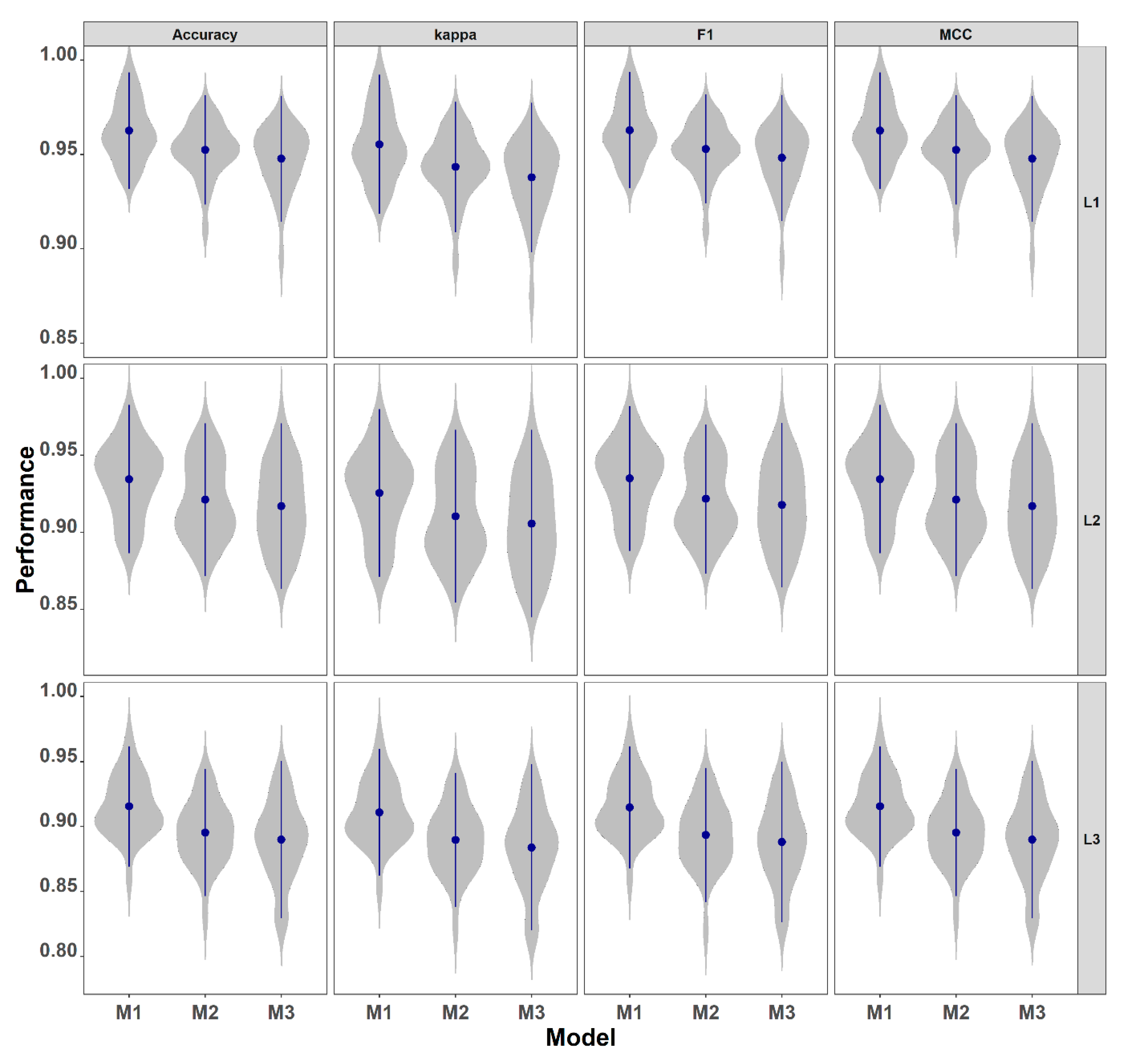
3.1.2. Effect of Classification Complexity

A second major pattern was the decrease in model performance with increasing thematic resolution. Across all model types, classification accuracy declined from L1 (9 classes) to L2 (14 classes), and further to L3 (23 classes) (Table 2). For the full model, overall accuracy decreased from 0.97 at L1 to 0.94 at L2, and 0.93 at L3. Similar declines were observed for kappa, weighted F1, and MCC. This trend reflects the increasing spectral and ecological similarity among classes at a higher classification detail, which presents greater challenges for model discrimination.

Despite this expected reduction in performance, the full model maintained high accuracy, even at the most detailed level. At L3, it achieved a kappa score of 0.92 and MCC of 0.92 (based on the testing confusion matrix in Supplementary Material S5), indicating reliable differentiation among vegetation types with overlapping spectral signatures and dynamic seasonal behaviors.

3.1.3. Statistical Comparison of Model Variants

Significance testing (

Table 3. Significance test results of the pairwise comparison between Random Forest classifiers with different levels of model complexity. Non-significant comparisons are in bold.

Levels	Pairs	Overall Accuracy		Kappa		Weigted F1		MCC
		Difference	p_Value	Difference	p_Value	Difference	p_Value	Difference	p_Value
L1	M1~M2	0.010	0.011	0.012	0.012	0.010	0.012	0.012	0.013
	M1~M3	0.015	0.001	0.018	0.001	0.015	0.001	0.017	0.001
	M1~M4	0.400	0.000	0.468	0.000	0.399	0.000	0.465	0.000
	M2~M3	0.005	0.240	0.006	0.244	0.005	0.235	0.005	0.258
	M2~M4	0.389	0.000	0.456	0.000	0.389	0.000	0.453	0.000
	M3~M4	0.385	0.000	0.450	0.000	0.384	0.000	0.448	0.000
L2	M1~M2	0.013	0.039	0.015	0.037	0.013	0.034	0.015	0.038
	M1~M3	0.018	0.010	0.020	0.009	0.017	0.012	0.020	0.010
	M1~M4	0.410	0.000	0.458	0.000	0.408	0.000	0.455	0.000
	M2~M3	0.004	0.521	0.005	0.523	0.004	0.533	0.005	0.537
	M2~M4	0.397	0.000	0.443	0.000	0.395	0.000	0.440	0.000
	M3~M4	0.393	0.000	0.438	0.000	0.391	0.000	0.436	0.000
L3	M1~M2	0.020	0.002	0.021	0.002	0.021	0.001	0.021	0.002
	M1~M3	0.026	0.001	0.027	0.001	0.027	0.001	0.027	0.001
	M1~M4	0.381	0.000	0.399	0.000	0.396	0.000	0.397	0.000
	M2~M3	0.005	0.429	0.006	0.436	0.005	0.453	0.006	0.437
	M2~M4	0.361	0.000	0.378	0.000	0.374	0.000	0.375	0.000
	M3~M4	0.356	0.000	0.372	0.000	0.369	0.000	0.370	0.000

) confirmed the superiority of the full model over more limited models. Pairwise comparisons showed that the full model (M1) significantly outperformed both the S1S2 (M2) and S2-only (M3) models across all metrics and classification levels, with p-values < 0.05 in most cases. Differences between M2 and M3 were generally not significant, indicating similar performance when excluding SAR data. The topography-only model (M4) was significantly inferior to all other models, with p-values < 0.001.

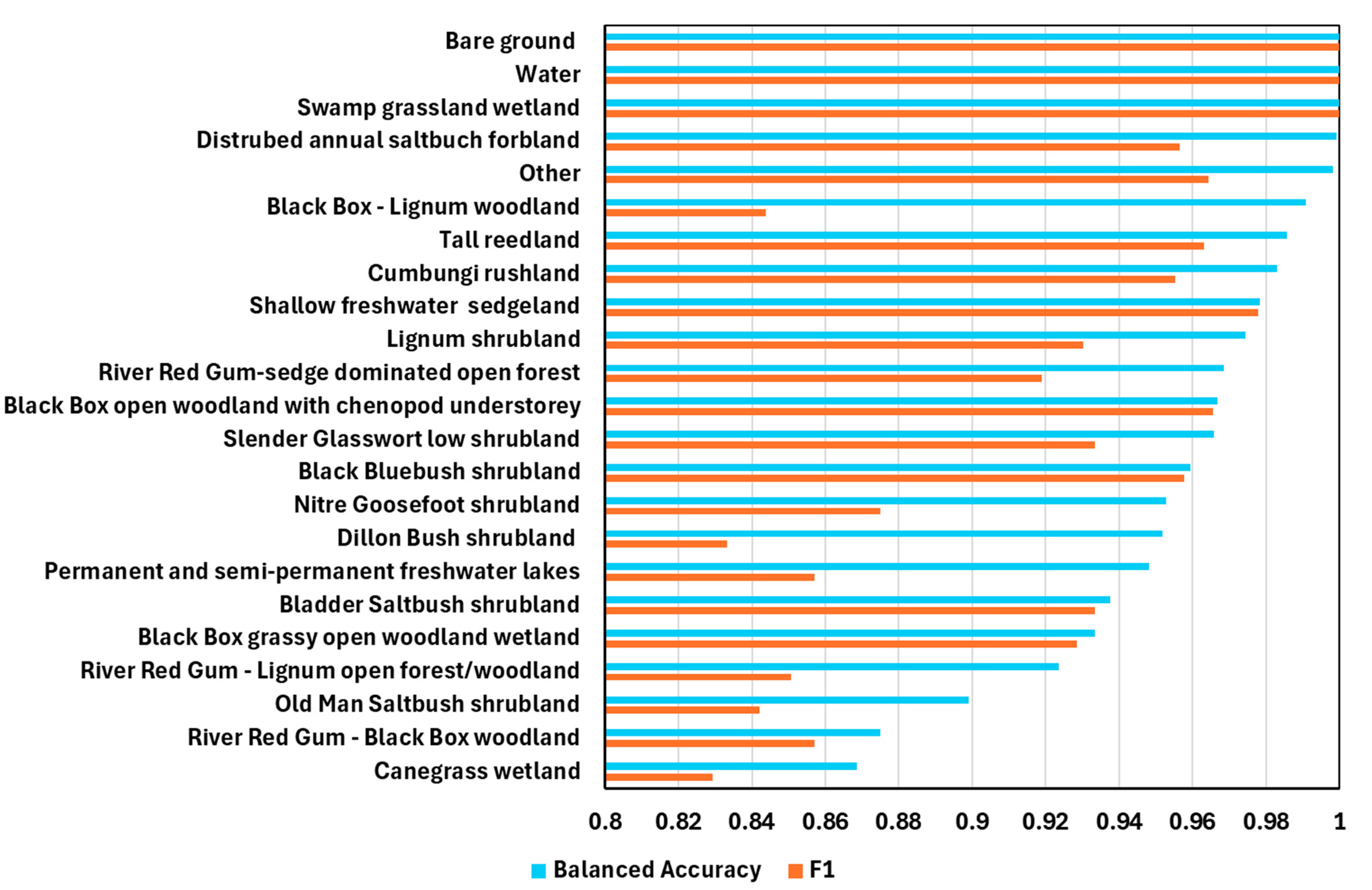
3.1.4. Model Assessment for Plant Community Types (PCTs)

The classification accuracy of the full model was further assessed at the most detailed level—plant community types (PCTs)—to evaluate its ability to resolve fine-scale vegetation patterns in a complex floodplain wetland. The results based on the independent test dataset showed that the model performed strongly across nearly all PCTs, with high balanced-accuracy and F1 scores observed even for the most challenging classes.

Several PCTs achieved near-perfect classification. Swamp Grassland Wetland, Water, and Bare Ground were classified with 100% balanced accuracy and F1 scores of 1.00 (Figure 4). These outcomes reflect the distinct spectral and temporal signatures of these categories. For example, water and bare ground have well-established separability in both SAR and optical reflectance domains, while Swamp Grassland Wetland likely exhibited stable seasonal phenology and minimal structural confusion.

The Cane-grass Wetland class had the lowest classification performance among the 23 PCTs, with a balanced accuracy of 0.87 and an F1 score of 0.83. However, even this represents a high level of classification accuracy when compared with similar studies in wetland environments, where class-specific F1 scores for detailed vegetation types often range between 0.70 and 0.85 [16,18]. The moderate reduction in accuracy for Cane-grass Wetland may be attributed to its spectral and structural similarity with adjacent communities such as Tall Marsh or Mixed Wetlands, as well as potential seasonal overlap in phenological characteristics. Misclassification may also be more likely where vegetation occurs in transitional zones or exhibits subdominant growth forms within mixed patches.

Despite this, the overall model performance at the PCT level remains robust. Most classes achieved F1 scores above 0.90, underscoring the model’s capacity to differentiate among ecologically and structurally similar vegetation communities. The consistently high accuracy across a large number of classes (n = 23) highlights the strength of combining SAR and optical time series data with hydro-morphological predictors and cluster-guided training. This approach not only captures spectral–temporal variation but also addresses structural and topographic differences that influence vegetation composition across the floodplain.

These findings reinforce that the proposed classification framework is capable of delivering fine-resolution vegetation maps with accuracy levels that meet or exceed those reported in comparable studies, even under challenging conditions of high class diversity, spatial complexity, and phenological variability.

Together, these results confirm that increasing the diversity of input features—particularly the inclusion of SAR and hydro-morphological variables—substantially improves classification accuracy. The combination of multi-platform data, phenological metrics, and terrain structure is especially valuable in heterogeneous floodplain systems, where subtle variations in vegetation are difficult to capture using spectral data alone.

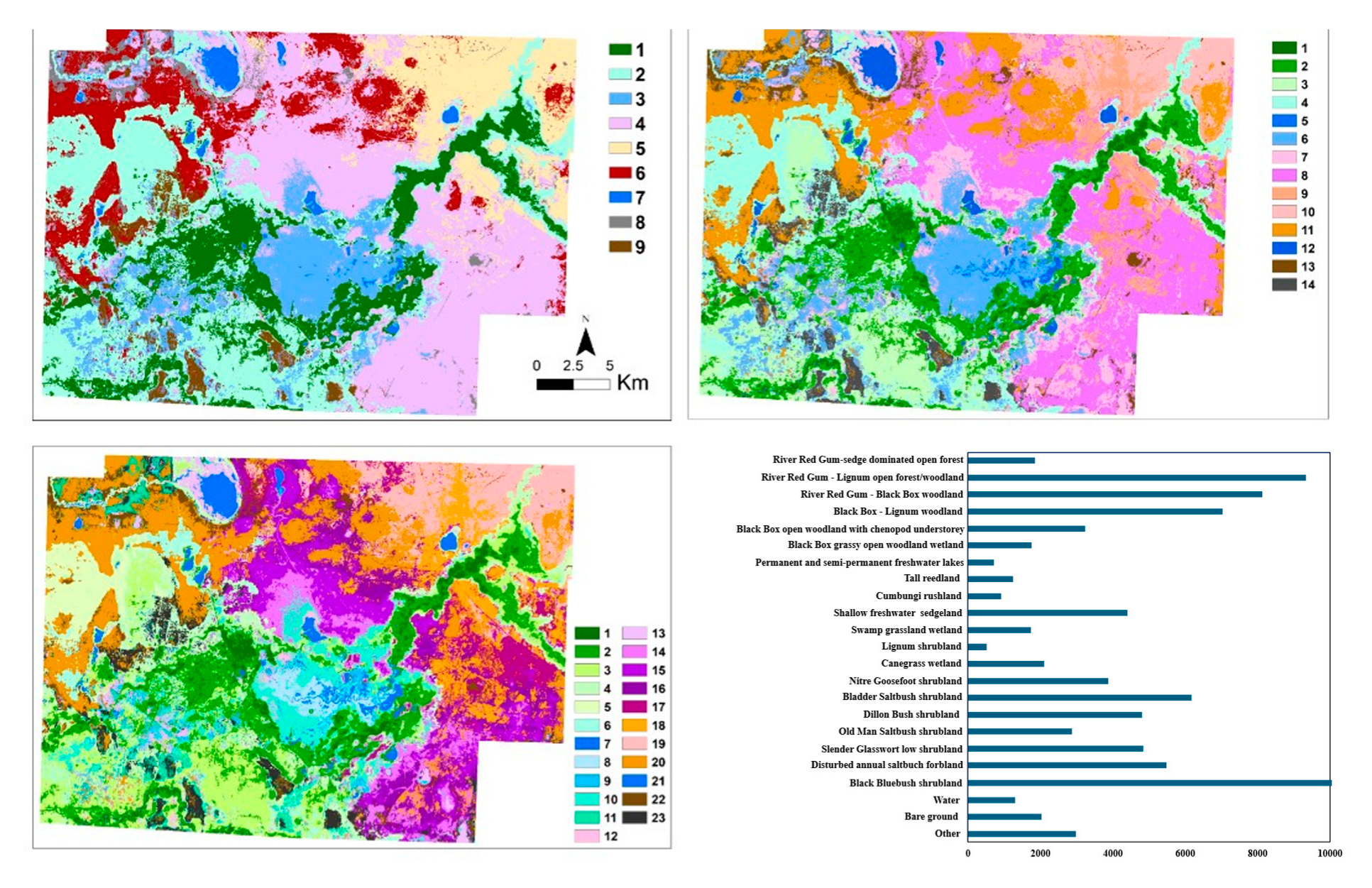
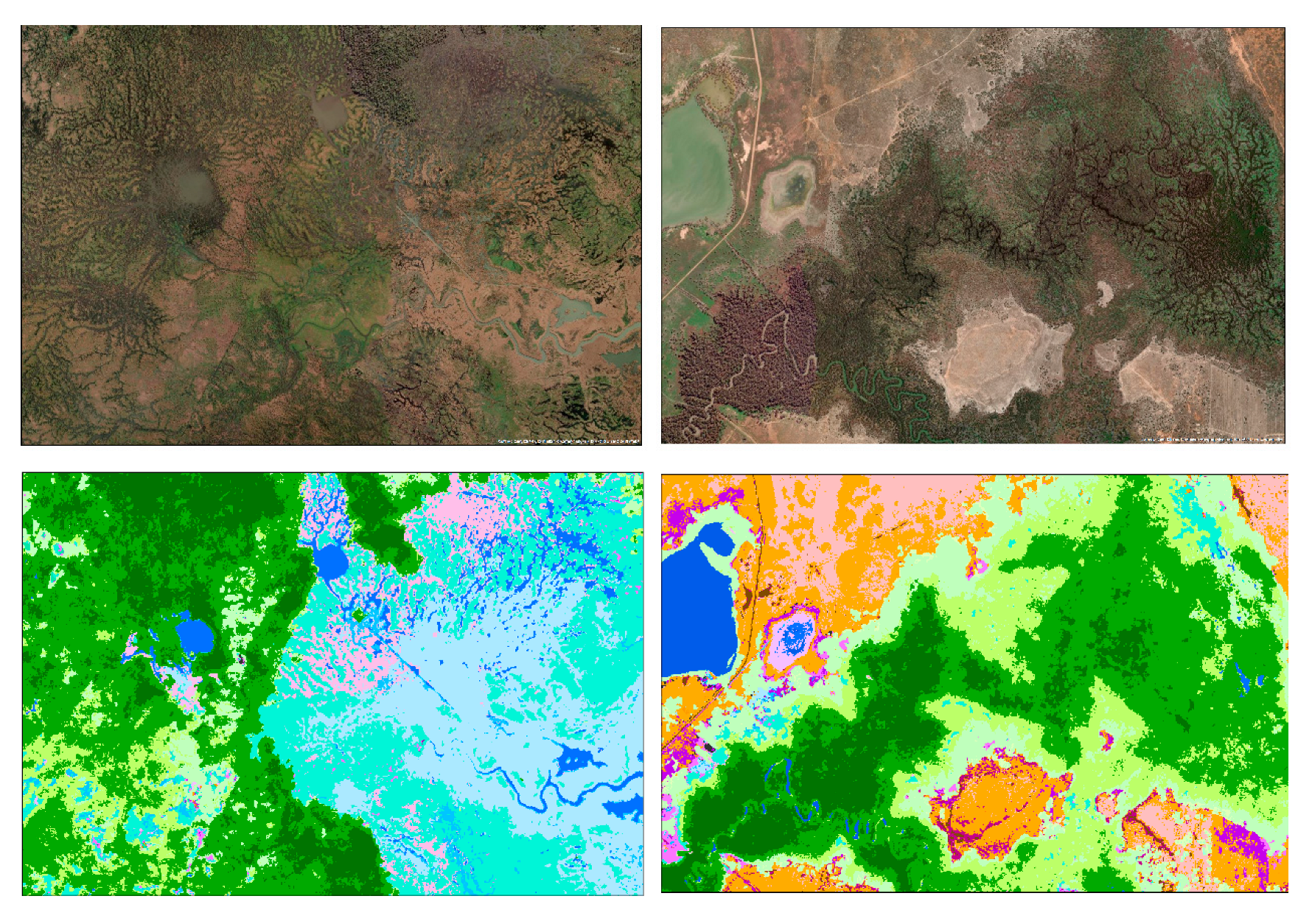
3.2. Vegetation Maps

The classification framework produced high-resolution vegetation maps at three ecological levels: foundational vegetation types (L1), functional groups (L2), and plant community types (PCTs; L3). These maps are presented in Figure 5. The total areas of the wetlands mapped in the Great Cumbung Swamp were 72,122 ha, 71,149 ha, and 71,078 ha under the Level 1, Level 2, and Level 3 classification schemes, respectively. Minor differences in total area reflect classification uncertainties at the margins and transitions between classes.

At the most detailed level (Level 3), 23 PCTs were delineated. The largest mapped vegetation assemblage was River Red Gum–Lignum open forest/woodland (9344 ha), followed by River Red Gum–Black Box woodland (8136 ha). In contrast, Lignum shrubland covered the smallest area, at 507 ha. The spatial distributions of these communities closely matched ecological expectations and available reference data.

The mapped vegetation classes at Level 3 aggregated well into broader categories at Level 2, which in turn aligned with Level 1 formations. For example, six Level 3 PCTs—River Red Gum–sedge dominated open forest, River Red Gum–Lignum open forest/woodland, River Red Gum–Black Box woodland, Black Box–Lignum woodland, Black Box open woodland with chenopod understorey, and Black Box grassy open woodland—together accounted for 31,374 ha. This was closely aligned with the 31,790 ha of woody wetlands (including forests and woodlands) mapped at Level 1. Such hierarchical consistency supports the ecological validity of the classification framework and demonstrates its scalability across multiple thematic resolutions.

Key wetland communities, which are also conservation targets, such as Phragmites australis-dominated reedbeds and Typha-dominated swamps were clearly distinguished and spatially coherent. Field validation and visual comparison with high-resolution aerial imagery confirmed the accuracy of mapped boundaries, particularly for complex or transitional habitats. Figure 6 illustrates a comparison between the predicted vegetation types and the 30 cm resolution aerial photographs captured on 8 November 2023, showing strong correspondence in both downstream and upstream zones of the Great Cumbung Swamp. The model successfully resolved subtle differences among grassy wetlands and riparian woodlands, including between spectrally similar classes such as Phragmites and Typha stands.

The Random Forest model achieved strong classification performance across all levels, with the full model (incorporating all 50 predictors) attaining over 90% overall accuracy even at the PCT level. This high accuracy is particularly notable given the spectral similarity and ecological overlap among many wetland vegetation classes. The combination of Sentinel-1 SAR, Sentinel-2 optical time series, terrain variables, and ecologically representative training data—selected through unsupervised clustering—proved highly effective for resolving these complexities. The integration of temporal and structural information, along with a cluster-guided sampling strategy, enabled the model to distinguish between ecologically distinct but spectrally confounded vegetation types that might otherwise be misclassified using conventional approaches.

4. Discussion

This study presents a robust and scalable framework for inland floodplain vegetation mapping that achieves high thematic resolution and classification accuracy while substantially reducing the need for costly field-based sampling. By leveraging unsupervised clustering for sample targeting [49] and integrating multi-source data—including Sentinel-1 SAR, Sentinel-2 optical time series, and hydro-morphological terrain metrics—our approach addresses several key limitations reported in the wetland remote-sensing literature [15,16,18,21].

4.1. Performance in the Context of Recent Studies

Accurate, high-resolution wetland vegetation mapping remains a persistent challenge due to complex landscape heterogeneity, hydrological variability, and spectral overlap among vegetation types. Numerous studies have made progress in this space, yet notable limitations persist when scaling to large floodplain systems or achieving high thematic resolution.

In terms of data sources, many previous wetland mapping studies have relied primarily on single-sensor optical data. For example, Lane et al. [21] used WorldView-2 imagery to map 22 vegetation types in freshwater wetlands, with an overall accuracy of 86.5%, while Bhatnagar et al. [18] achieved up to 87% accuracy for 18 wetland communities in Ireland, using Sentinel-2 data alone. Although these studies demonstrated the potential of high-resolution optical imagery, reliance on optical data limits performance in areas with persistent cloud cover, coarse vegetation structure, or subtle spectral differences between classes.

The approach presented in this study improves upon these limitations by integrating multi-temporal Sentinel-1 SAR, Sentinel-2 optical data, and hydro-morphological predictors derived from LiDAR and a SRTM-fused high-resolution DEM. This multi-source data fusion enhances the ability to discriminate vegetation types, using not only spectral and phenological properties but also structural and topographic characteristics, which are particularly important in hydrologically dynamic floodplain environments like the Great Cumbung Swamp.

Methodologically, traditional supervised classification approaches in wetland studies often rely heavily on extensive, well-distributed field data for model training [16,19,20]. In contrast, this study introduces an unsupervised cluster-guided sample selection strategy, which, when combined with expert labeling, significantly reduces dependence on large-scale field campaigns. This addresses a key logistical constraint relevant to remote or inaccessible wetland landscapes, while still producing high-quality, representative training data for classification.

In terms of classification accuracy, the framework achieved overall accuracies exceeding 90% across all three hierarchical levels, with the detailed plant community type (PCT) classification reaching an overall accuracy of 93.2%, a kappa coefficient of 0.91, and a Matthews correlation coefficient (MCC) of 0.89. These results surpass many previously published wetland vegetation mapping efforts, particularly those involving complex, multi-class classifications exceeding 20 vegetation types.

Collectively, the combination of multi-source data fusion, reduced field data requirements, and high classification accuracy demonstrated in this study represents a significant advancement for scalable, high-resolution wetland vegetation mapping. The methodological innovations improve the practicality and cost-effectiveness of applying detailed vegetation mapping to large, heterogeneous inland floodplain systems, providing critical tools for conservation planning, ecological monitoring, and wetland management.

4.2. Advantages of the Sequential Clustering–Labeling–Classification Approach

A key innovation of this study is the sequential use of clustering, expert-guided labeling, and supervised classification. This framework provides several distinct advantages.

4.2.1. Refining Training Data Quality

Clustering—especially using unsupervised K-means—allows for refinement of training data by grouping spectrally and temporally consistent pixels. This reduces the inclusion of ambiguous or misclassified pixels, which is especially important when training data are derived from legacy LULC datasets or limited field data [49]. The result is a cleaner and more representative training dataset that enhances classification performance.

4.2.2. Reducing Intra-Class Variability and Spectral Noise

Grouping similar pixels before classification reduces within-class spectral variability. This helps overcome the “salt-and-pepper” noise often observed in pixel-based classifications [50]. When combined with segmentation techniques in object-based image analysis (OBIA) [51,52], clusters can be used to define ecologically meaningful spatial units that capture texture, shape, and contextual information [53].

4.2.3. Improving Delineation of Vegetation Boundaries

The use of image objects or spectral-temporal clusters improves the detection of vegetation transitions and boundary accuracy. Integrating segmentation with deep learning architectures like DeepLabV3+ has been shown to correct misclassifications at edges and reduce spatial fragmentation [54,55], further supporting the value of this workflow.

While deep learning approaches such as U-Net and other convolutional neural networks (CNNs) have shown great promise for vegetation classification and boundary delineation, they typically require large, well-labeled training datasets and substantial computational resources [56]. This can present significant challenges for wetland mapping in remote or data-scarce regions. Although deep learning models may offer enhanced boundary precision under optimal conditions, our framework provides a more accessible and scalable alternative, one particularly suited to heterogeneous landscapes where field data collection is logistically or financially constrained. Moreover, the cluster-guided sample selection used in this study addresses a key limitation of many machine learning and deep learning applications by improving training data quality while minimizing ground survey demands. Future research could explore the integration of object-based segmentation with deep learning to combine the strengths of both approaches, enhancing boundary accuracy while maintaining efficiency in training data requirements.

4.3. Implications and Transferability

This approach is especially valuable for ecological monitoring in remote, heterogeneous, or data-scarce landscapes. The framework is readily transferable to other wetland systems with similar challenges, such as seasonal flooding, spectral overlap, and limited ground-truth data. Its compatibility with cloud-based platforms like Google Earth Engine enables efficient implementation across large regions and time periods, allowing for cost-effective repeat monitoring [57].

The cluster-guided sampling method is particularly suited to conservation applications, as it enables high-quality map outputs with minimal field effort. This supports land managers and policymakers seeking to identify priority areas for restoration, monitor compliance with environmental water delivery, or assess changes in wetland condition.

An important practical consideration is whether classification at the highest thematic resolution—the plant community type (PCT) level—offers a more efficient workflow, even though its accuracy is lower than those found in broader categories such as functional groups or formations. Given the nested, hierarchical structure of the classification system, accurate prediction at the PCT level intrinsically provides the corresponding functional group and formation information. This approach would allow for all three classification levels to be derived in a single processing step, reducing computational effort and simplifying model implementation.

While classification accuracy typically declines as thematic detail increases, the PCT-level accuracy achieved in this study remains high, exceeding those of many comparable multi-class wetland mapping efforts. Future work could formally test this hierarchical workflow by comparing derived functional group and formation maps from PCT predictions against independently generated models at each level, providing practical insights into trade-offs between accuracy, efficiency, and thematic resolution.

Although this study focused on the Great Cumbung Swamp, the proposed framework is designed to be broadly transferable to other wetland or floodplain systems. The integration of multi-temporal satellite data, hydro-morphological predictors, and cluster-guided sample selection does not rely on site-specific conditions, making the approach adaptable to landscapes with varying geomorphology, vegetation complexity, or climate regimes. However, transferability is likely to depend on the availability and quality of input data, particularly high-resolution terrain information and appropriately calibrated remote-sensing imagery. In environments that are more topographically complex or hydrologically distinct, adjustments to predictor selection or model tuning may be required to account for local ecological drivers. Future research applying this framework across contrasting wetland types—such as arid-zone floodplains, coastal marshes, or peatlands—would help to further assess its generalizability and refine best practices for scalable wetland vegetation mapping [56].

4.4. Future Directions in Wetland Vegetation Classification

Future advances in wetland vegetation classification will be shaped by the integration of artificial intelligence, multi-source data, and scalable computing platforms. Deep learning methods, particularly convolutional neural networks (CNNs) and segmentation models like U-Net, have shown strong potential for automating feature extraction and improving boundary accuracy [57,58,59]. When combined with object-based image analysis (OBIA), these approaches can reduce classification noise and improve spatial coherence, especially in structurally complex wetlands [50,57].

Leveraging time-series data to capture phenological variation [27,60] is another promising direction. Seasonal dynamics in wetland vegetation can be exploited through harmonic analysis and temporal kernels, enhancing the discrimination of spectrally similar species [18]. High-revisit sensors such as PlanetScope and Sentinel-2 provide the temporal resolution needed to detect key phenological phases, offering improved classification accuracy during optimal seasonal windows.

Model transparency remains a challenge, particularly with deep learning models. Tools such as Shapley Additive Explanations (SHAP) can improve interpretability by identifying the contribution of individual features to model predictions [61], making AI outputs more accessible to ecologists and resource managers [56,62].

Scaling models across different regions and vegetation types will require advances in transfer learning and semi-supervised approaches, especially in data-scarce areas. Continued improvements in remote-sensing technology—including hyperspectral and LiDAR sensors—will further support species- and trait-level classification [63], while cloud platforms like Google Earth Engine will facilitate efficient, large-scale processing [55].

Looking forward, integrating classification outputs with ecosystem function metrics—such as biomass, evapotranspiration, and responses to hydrological variability—will be essential for tracking long-term wetland dynamics under climate change. Together, these innovations point toward a future of more accurate, interpretable, and scalable wetland vegetation monitoring.

5. Conclusions

This study presents a robust and scalable framework for inland floodplain vegetation mapping that achieves high thematic resolution and classification accuracy, while reducing reliance on extensive field-based sampling for model training. Nonetheless, field data remain essential for defining classification schemes, guiding sample selection, and providing independent validation. By combining unsupervised clustering, expert-guided sample refinement, and multi-source remote-sensing data, the framework achieved high classification accuracy across more than 20 vegetation classes, surpassing the performance reported in many recent studies. The approach not only enhances classification performance but also reduces the dependency on extensive field data collection, making it especially valuable in remote or under-surveyed regions.

The resulting high-resolution vegetation maps provide critical insights for wetland conservation and management. These maps can inform environmental water allocations, support the design of ecological monitoring programs, guide restoration planning, and contribute to the protection of wetland-dependent biodiversity. More broadly, they enable adaptive management by offering spatially explicit data on vegetation structure, composition, and dynamics—key indicators of wetland condition and ecological integrity.

As satellite data availability, computational capacity, and AI capabilities continue to expand, frameworks such as the one presented here will become increasingly important for ecosystem-scale monitoring. Future work should focus on integrating structural, phenological, and functional data to move beyond static classification and toward dynamic, continuous monitoring systems that support long-term conservation and sustainable wetland management.

References

1. Kingsford, R.T.; Basset, A.; Jackson, L. Wetlands: Conservation’s poor cousins. Aquat. Conserv. Mar. Freshw. Ecosyst. 2016, 26, 892–916. [Google Scholar] [CrossRef]
2. Junk, W.J.; An, S.; Finlayson, C.M.; Gopal, B.; Květ, J.; Mitchell, S.A.; Mitsch, W.J.; Robarts, R.D. Current state of knowledge regarding the world’s wetlands and their future under global climate change: A synthesis. Aquat. Sci. 2013, 75, 151–167. [Google Scholar] [CrossRef]
3. Bhowmik, S. Ecological and economic importance of wetlands and their vulnerability: A review. In Research Anthology on Ecosystem Conservation and Preserving Biodiversity; IGI Publication: Hershey, PA, USA, 2022; pp. 11–27. [Google Scholar]
4. Dar, S.A.; Bhat, S.U.; Rashid, I.; Dar, S.A. Current status of wetlands in Srinagar City: Threats, management strategies, and future perspectives. Front. Environ. Sci. 2020, 7, 199. [Google Scholar] [CrossRef]
5. Newton, A.; Icely, J.; Cristina, S.; Perillo, G.M.; Turner, R.E.; Ashan, D.; Cragg, S.; Luo, Y.; Tu, C.; Li, Y.; et al. Anthropogenic, direct pressures on coastal wetlands. Front. Ecol. Evol. 2020, 8, 144. [Google Scholar] [CrossRef]
6. Doody, T.M.; McInerney, P.J.; Thoms, M.C.; Gao, S. Resilience and adaptive cycles in water-dependent ecosystems: Can panarchy explain trajectories of change among floodplain trees? In Resilience and Riverine Landscapes; Elsevier: Amsterdam, The Netherlands, 2024; pp. 97–115. [Google Scholar]
7. Keddy, P.A.; Fraser, L.H.; Solomeshch, A.I.; Junk, W.J.; Campbell, D.R.; Arroyo, M.T.; Alho, C.J. Wet and wonderful: The world’s largest wetlands are conservation priorities. BioScience 2009, 59, 39–51. [Google Scholar] [CrossRef]
8. Thamaga, K.H.; Dube, T.; Shoko, C. Advances in satellite remote sensing of the wetland ecosystems in Sub-Saharan Africa. Geocarto Int. 2022, 37, 5891–5913. [Google Scholar] [CrossRef]
9. Sun, W.; Chen, D.; Li, Z.; Li, S.; Cheng, S.; Niu, X.; Cai, Y.; Shi, Z.; Wu, C.; Yang, G.; et al. Monitoring wetland plant diversity from space: Progress and perspective. Int. J. Appl. Earth Obs. Geoinf. 2024, 130, 103943. [Google Scholar] [CrossRef]
10. Jones, H.G.; Vaughan, R.A. Remote Sensing of Vegetation: Principles, Techniques, and Applications; Oxford University Press: Oxford, UK, 2010. [Google Scholar]
11. Wang, Y.; Gong, Z.; Zhou, H. Long-term monitoring and phenological analysis of submerged aquatic vegetation in a shallow lake using time-series imagery. Ecol. Indic. 2023, 154, 110646. [Google Scholar] [CrossRef]
12. McCarthy, M.J.; Radabaugh, K.R.; Moyer, R.P.; Muller-Karger, F.E. Enabling efficient, large-scale high-spatial resolution wetland mapping using satellites. Remote Sens. Environ. 2018, 208, 189–201. [Google Scholar] [CrossRef]
13. Mansaray, A.S.; Dzialowski, A.R.; Martin, M.E.; Wagner, K.L.; Gholizadeh, H.; Stoodley, S.H. Comparing PlanetScope to Landsat-8 and Sentinel-2 for sensing water quality in reservoirs in agricultural watersheds. Remote Sens. 2021, 13, 1847. [Google Scholar] [CrossRef]
14. Pan, B.; Xiao, X.; Luo, S.; Pan, L.; Yao, Y.; Zhang, C.; Meng, C.; Qin, Y. Identify and track white flower and leaf phenology of deciduous broadleaf trees in spring with time series PlanetScope images. ISPRS J. Photogramm. Remote Sens. 2025, 226, 127–145. [Google Scholar] [CrossRef]
15. Lamb, B.T.; Tzortziou, M.A.; McDonald, K.C. Evaluation of approaches for mapping tidal wetlands of the Chesapeake and Delaware Bays. Remote Sens. 2019, 11, 2366. [Google Scholar] [CrossRef]
16. Niculescu, S.; Boissonnat, J.B.; Lardeux, C.; Roberts, D.; Hanganu, J.; Billey, A.; Constantinescu, A.; Doroftei, M. Synergy of high-resolution radar and optical images satellite for identification and mapping of wetland macrophytes on the Danube Delta. Remote Sens. 2020, 12, 2188. [Google Scholar] [CrossRef]
17. Hubert-Moy, L.; Fabre, E.; Rapinel, S. Contribution of SPOT-7 multi-temporal imagery for mapping wetland vegetation. Eur. J. Remote Sens. 2020, 53, 201–210. [Google Scholar] [CrossRef]
18. Bhatnagar, S.; Gill, L.; Regan, S.; Naughton, O.; Johnston, P.; Waldren, S.; Ghosh, B. Mapping vegetation communities inside wetlands using sentinel-2 imagery in Ireland. Int. J. Appl. Earth Obs. Geoinf. 2020, 88, 102083. [Google Scholar] [CrossRef]
19. Wen, L.; Hughes, M. Coastal wetland mapping using ensemble learning algorithms: A comparative study of bagging, boosting and stacking techniques. Remote Sens. 2020, 12, 1683. [Google Scholar] [CrossRef]
20. Mutanga, O.; Adam, E.; Cho, M.A. High density biomass estimation for wetland vegetation using WorldView-2 imagery and random forest regression algorithm. Int. J. Appl. Earth Obs. Geoinf. 2012, 18, 399–406. [Google Scholar] [CrossRef]
21. Lane, C.; Liu, H.; Autrey, B.; Anenkhonov, O.; Chepinoga, V.; Wu, Q. Improved Wetland Classification Using Eight-Band High Resolution Satellite Imagery and a Hybrid Approach. Remote Sens. 2014, 6, 12187–12216. [Google Scholar] [CrossRef]
22. MacQueen, J. Some Methods for Classification and Analysis of Multivariate Observations. In Proceedings of the Fifth Berkeley Symposium on Mathematical Statistics and Probability; University of California Press: Berkeley, CA, USA, 1967; Volume 1, pp. 281–297. [Google Scholar]
23. Hastie, T.; Tibshirani, R.; Friedman, J. The Elements of Statistical Learning: Data Mining, Inference, and Prediction; Springer: Berlin/Heidelberg, Germany, 2009. [Google Scholar]
24. Zhu, X. Semi-Supervised Learning Literature Survey. In Computer Sciences Technical Report 1530; University of Wisconsin-Madison: Madison, WI, USA, 2005. [Google Scholar]
25. Chapelle, O.; Scholkopf, B.; Zien, A. Semi-Supervised Learning; MIT Press: Cambridge, MA, USA, 2006. [Google Scholar]
26. Dronova, I.; Gong, P.; Wang, L. Object-based analysis and change detection of major wetland cover types and their classification uncertainty during the low water period at Poyang Lake, China. Remote Sens. Environ. 2011, 115, 3220–3236. [Google Scholar] [CrossRef]
27. Viana, C.M.; Girão, I.; Rocha, J. Long-term satellite image time-series for land use/land cover change detection using refined open source data in a rural region. Remote Sens. 2019, 11, 1104. [Google Scholar] [CrossRef]
28. Higgisson, W.; Cobb, A.; Tschierschke, A.; Dyer, F. The role of environmental water and reedbed condition on the response of Phragmites australis reedbeds to flooding. Remote Sens. 2022, 14, 1868. [Google Scholar] [CrossRef]
29. Dyer, F.; Broadhurst, B.; Tschierschke, A.; Higgisson, W.; Allan, H.; Thiem, J.; Wright, D.; Thompson, R. Commonwealth Environmental Water Office Long Term Intervention Monitoring Project: Lachlan River System Selected Area 2018-19 Monitoring and Evaluation Summary Report; Commonwealth Environmental Water Holder: Canberra, Australia, 2019. [Google Scholar]
30. DEECCW. Plan to Protect the Great Cumbung Swamp. 2023. Available online: https://www.dcceew.gov.au/cewh/resources-media/news/plan-to-protect-the-great-cumbung-swamp (accessed on 12 February 2025).
31. Pfitzner, K.; Bartolo, R.; Whiteside, T.; Loewensteiner, D.; Esparon, A. Multi-temporal spectral reflectance of tropical savanna understorey species and implications for hyperspectral remote sensing. Int. J. Appl. Earth Obs. Geoinf. 2022, 112, 102870. [Google Scholar] [CrossRef]
32. Chen, Y.; Cao, R.; Chen, J.; Liu, L.; Matsushita, B. A practical approach to reconstruct high-quality Landsat NDVI time-series data by gap filling and the Savitzky–Golay filter. ISPRS J. Photogramm. Remote Sens. 2021, 180, 174–190. [Google Scholar] [CrossRef]
33. Liu, X.; Zhai, H.; Shen, Y.; Lou, B.; Jiang, C.; Li, T.; Hussain, S.B.; Shen, G. Large-scale crop mapping from multisource remote sensing images in google earth engine. IEEE J. Sel. Top. Appl. Earth Obs. Remote Sens. 2020, 13, 414–427. [Google Scholar] [CrossRef]
34. Montero, D.; Aybar, C.; Mahecha, M.D.; Martinuzzi, F.; Söchting, M.; Wieneke, S. A standardized catalogue of spectral indices to advance the use of remote sensing in Earth system research. Sci. Data 2023, 10, 197. [Google Scholar] [CrossRef]
35. Geoscience Australia. Digital Elevation Model (DEM) of Australia Derived from LiDAR 5 Metre Grid; Geoscience Australia: Canberra, Australia, 2015.
36. Pedersen, E.J.; Miller, D.L.; Simpson, G.L.; Ross, N. Hierarchical generalized additive models in ecology: An introduction with mgcv. PeerJ 2019, 7, e6876. [Google Scholar] [CrossRef]
37. Gallant, J.C.; Dowling, T.I.; Read, A.M.; Wilson, N.; Tickle, P.K.; Inskeep, C. 1 Second SRTM-Derived Digital Elevation Models User Guide. Geoscience Australia. 2011. Available online: www.ga.gov.au/topographic-mapping/digital-elevation-data.html (accessed on 2 June 2025).
38. Brown, C.F.; Brumby, S.P.; Guzder-Williams, B.; Birch, T.; Hyde, S.B.; Mazzariello, J.; Czerwinski, W.; Pasquarella, V.J.; Haertel, R.; Ilyushchenko, S.; et al. Dynamic World, Near real-time global 10 m land use land cover mapping. Sci. Data 2022, 9, 251. [Google Scholar] [CrossRef]
39. Shrestha, N. Detecting multicollinearity in regression analysis. Am. J. Appl. Math. Stat. 2020, 8, 39–42. [Google Scholar] [CrossRef]
40. Kuhn, M. Building predictive models in R using the caret package. J. Stat. Softw. 2008, 28, 1–26. [Google Scholar] [CrossRef]
41. R Development Core Team. R: A Language and Environment for Statistical Computing; R Foundation for Statistical Computing: Vienna, Austria, 2023; ISBN 3-900051-07-0. [Google Scholar]
42. Baldi, P.; Brunak, S.; Chauvin, Y.; Andersen, C.A.; Nielsen, H. Assessing the accuracy of prediction algorithms for classification: An overview. Bioinformatics 2000, 16, 412–424. [Google Scholar] [CrossRef]
43. Chicco, D.; Jurman, G. The advantages of the Matthews correlation coefficient (MCC) over F1 score and accuracy in binary classification evaluation. BMC Genom. 2020, 21, 6. [Google Scholar] [CrossRef]
44. Janssen, L.L.; Vanderwel, F.J. Accuracy assessment of satellite derived land-cover data: A review. Photogramm. Eng. Remote Sens. 1994, 60, 419–426. [Google Scholar]
45. Liu, C.; Frazier, P.; Kumar, L. Comparative assessment of the measures of thematic classification accuracy. Remote Sens. Environ. 2007, 107, 606–616. [Google Scholar] [CrossRef]
46. Harbecke, D.; Chen, Y.; Hennig, L.; Alt, C. Why only micro-f1? class weighting of measures for relation classification. arXiv 2022, arXiv:2205.09460. [Google Scholar]
47. Chicco, D.; Tötsch, N.; Jurman, G. The Matthews correlation coefficient (MCC) is more reliable than balanced accuracy, bookmaker informedness, and markedness in two-class confusion matrix evaluation. BioData Min. 2021, 14, 13. [Google Scholar] [CrossRef]
48. Yan, Y. MLmetrics: Machine Learning Evaluation Metrics; R Package Version 1.1.1; R Foundation for Statistical Computing: Vienna, Austria, 2016. [Google Scholar]
49. Böge, M.; Bulatov, D.; Debroize, D.; Häufel, G.; Lucks, L. Efficient training data generation by clustering-based classification. ISPRS Annals of the Photogrammetry. Remote Sens. Spat. Inf. Sci. 2022, 3, 179–186. [Google Scholar]
50. Blaschke, T. Object based image analysis for remote sensing. ISPRS J. Photogramm. Remote Sens. 2010, 65, 2–16. [Google Scholar] [CrossRef]
51. Phiri, D.; Simwanda, M.; Salekin, S.; Nyirenda, V.R.; Murayama, Y.; Ranagalage, M. Sentinel-2 data for land cover/use mapping: A review. Remote Sens. 2020, 12, 2291. [Google Scholar] [CrossRef]
52. Dronova, I.; Gong, P.; Wang, L.; Zhong, L. Mapping dynamic cover types in a large seasonally flooded wetland using extended principal component analysis and object-based classification. Remote Sens. Environ. 2015, 158, 193–206. [Google Scholar] [CrossRef]
53. Ma, L.; Liu, Y.; Zhang, X.; Ye, Y.; Yin, G.; Johnson, B.A. Deep learning in remote sensing applications: A meta-analysis and review. ISPRS J. Photogramm. Remote Sens. 2019, 152, 166–177. [Google Scholar] [CrossRef]
54. Du, S.; Du, S.; Liu, B.; Zhang, X. Incorporating DeepLabv3+ and object-based image analysis for semantic segmentation of very high resolution remote sensing images. Int. J. Digit. Earth 2021, 14, 357–378. [Google Scholar] [CrossRef]
55. Gonçalves, J.; Pôças, I.; Marcos, B.; Mücher, C.A.; Honrado, J.P. SegOptim—A new R package for optimizing object-based image analyses of high-spatial resolution remotely-sensed data. Int. J. Appl. Earth Obs. Geoinf. 2019, 76, 218–230. [Google Scholar] [CrossRef]
56. Gorelick, N.; Hancher, M.; Dixon, M.; Ilyushchenko, S.; Thau, D.; Moore, R. Google Earth Engine: Planetary-scale geospatial analysis for everyone. Remote Sens. Environ. 2017, 202, 18–27. [Google Scholar] [CrossRef]
57. Li, X.; Tian, J.; Li, X.; Yu, Y.; Ou, Y.; Zhu, L.; Zhu, X.; Zhou, B.; Gong, H. Annual mapping of Spartina alterniflora with deep learning and spectral-phenological features from 2017 to 2021 in the mainland of China. Int. J. Remote Sens. 2024, 45, 3172–3199. [Google Scholar] [CrossRef]
58. Zhu, X.X.; Tuia, D.; Mou, L.; Xia, G.S.; Zhang, L.; Xu, F.; Fraundorfer, F. Deep learning in remote sensing: A comprehensive review and list of resources. IEEE Geosci. Remote Sens. Mag. 2017, 5, 8–36. [Google Scholar] [CrossRef]
59. Sakamoto, T.; Yokozawa, M.; Toritani, H.; Shibayama, M.; Ishitsuka, N.; Ohno, H. A crop phenology detection method using time-series MODIS data. Remote Sens. Environ. 2005, 96, 366–374. [Google Scholar] [CrossRef]
60. Zhang, Y.; Wu, Y.; Tong, K.; Chen, H.; Yuan, Y. Review of visual simultaneous localization and mapping based on deep learning. Remote Sens. 2023, 15, 2740. [Google Scholar] [CrossRef]
61. Zhou, Y.; Wu, W.; Wang, H.; Zhang, X.; Yang, C.; Liu, H. Identification of soil texture classes under vegetation cover based on Sentinel-2 data with SVM and SHAP techniques. IEEE J. Sel. Top. Appl. Earth Obs. Remote Sens. 2022, 15, 3758–3770. [Google Scholar] [CrossRef]
62. Lundberg, S.M.; Lee, S.I. A unified approach to interpreting model predictions. In Advances in Neural Information Processing Systems 30, Proceedings of the 31st Annual Conference on Neural Information Processing Systems (NIPS 2017), Long Beach, CA, USA, 4–9 December2017; Curran Associates Inc.: Red Hook, NY, USA, 2018. [Google Scholar]
63. Fu, B.; Deng, L.; Sun, W.; He, H.; Li, H.; Wang, Y.; Wang, Y. Quantifying vegetation species functional traits along hydrologic gradients in karst wetland based on 3D mapping with UAV hyperspectral point cloud. Remote Sens. Environ. 2024, 307, 114160. [Google Scholar] [CrossRef]
Figure 1. Vegetation samples in the Great Cumbung Swamp, located in the lower Lachlan River. The background features a gap-filled 5 m DEM, used to calculate 20 hydro-geomorphic variables. The inset map highlights the study site at the confluence of the Lachlan and Murrumbidgee Rivers, two major river systems in the Murray–Darling Basin, Australia.
Remotesensing 17 02279 g001
Figure 2. Modelling framework for wetland vegetation community classification. Vegetation indices and hydro-morphological variables used in this study are listed in Supplementary Material S1 and S2, respectively.
Remotesensing 17 02279 g002
Figure 3. Violin plots of the training performance distribution of the Random Forest classifiers. The dots and vertical bars are the mean and standard deviation of the 30 final models (3 repeats and 10 times). The performance results of the models with topographic variables only were much inferior (Table 2) and are excluded from the plots.
Remotesensing 17 02279 g003
Figure 4. Model performance for each plant community type. Data only shows the full model, which has the highest accuracy.
Remotesensing 17 02279 g004
Figure 5. Predicted vegetation maps for the Great Cumbung Swamp. From top right: vegetation formation (9 classes), functional groups (14 classes), PCT (23 classes), and the mapped area of each PCT. Refer to Table 1 for the names of vegetation classes.
Remotesensing 17 02279 g005
Figure 6. Comparison of aerial photographs (30 cm resolution, taken on 8 November 2023) and detailed VCT classifications of downstream (left) and upstream (right) of the Great Cumbung Swamp. The fitted RF model is capable of discriminating the subtle differences in grassy wetlands (e.g., Typha-dominated and Phragmites-dominated) and forests and woodland.
Remotesensing 17 02279 g006