Spatial Variation and Uncertainty Analysis of Black Sea Level Change from Virtual Altimetry Stations over 1993–2020

Abstract

Global mean sea level has been rising steadily since the early 1990s, yet regional sea level changes exhibit complex spatial variability that frequently contrasts with global trends. Investigating sea level variations in semi-enclosed basins such as the Black Sea is crucial for elucidating regional responses to climate change and characterizing its unique spatiotemporal evolution patterns. In this study, we employ satellite altimetry (SA) data to study sea level changes, spatial variability, and seasonal patterns in the Black Sea over eight distinct time periods with temporally correlated noise, and our results show good consistency with existing studies. The results show that sea level changes are non-linear over time and exhibit spatial variability in the Black Sea. The estimated sea level trend fluctuates over brief intervals, but extended time series provide reduced uncertainty in the trend and more precise estimation over a 28-year time series. The annual amplitude and phase derived from virtual altimetry data (1993–2020) exhibit a distinct seasonal pattern, with peak sea levels typically occurring between November and February. Furthermore, to reduce the uncertainty induced by noise in the sea surface height (SSH) time series, principal component analysis (PCA) was utilized to denoise the SSH data from 1993 to 2020, yielding a sea level trend of 1.76 ± 0.56 mm/yr. Denoising reduced the trend uncertainty by 57%, decreased the root mean square error of the SSH series by 5.06 mm, and decreased the annual amplitude by 23.35%.

1. Introduction

Sea levels exhibit temporal variations due to natural and anthropogenic factors. The primary factors influencing the current sea level change include glacier mass, tectonic activity, and geoid deformation, as well as greenhouse gas emissions [1,2,3,4]. Rising sea levels have emerged as an increasingly critical global issue owing to persistent global warming [5,6,7]. Since the 1990s, the global mean sea level has been increasing at an average rate of approximately 3.1 mm/yr [8,9,10]. The increase in sea levels has submerged low-lying coastal zones, amplified storm surge intensity, and accelerated coastal erosion and flood frequency, significantly threatening the long-term sustainability of coastal nations and communities [11,12].

The global trend of sea level rise frequently obscures the complexity of regional sea level variations, which exhibit spatial and temporal disparities. Consequently, while evaluating the possible effects of sea level rise on coastal areas, it is essential to concentrate on regional variations in sea level. The Black Sea (Figure 1), located in the southwestern region of Eurasia, represents the world’s largest inland marine basin by surface area. This semi-enclosed sea is bounded by six littoral states—Bulgaria, Romania, Ukraine, Russia, Georgia, and Turkey—serving as a strategic maritime nexus [13]. The Black Sea is fed by numerous significant river systems in Eastern Europe, namely the Danube, Dnieper, and Dniester rivers. In contrast to open ocean basins, it is hydrologically linked to the Sea of Azov through the Kerch Strait to the north and exchanges water with the global ocean via the narrow Turkish Straits in the southwest [14,15]. The Black Sea has a total coastline of around 4090 km. Coastal erosion and saltwater intrusion constitute significant environmental threats to adjacent regions. Prolonged alterations in water levels within the Black Sea have led to significant coastal transgression and regression. As marine forces increasingly affect low-lying coastal zones, the progressing erosional processes lead to the loss of beach areas, a landward displacement of the coastline, and the degradation of coastal ecosystems [16,17].

The Black Sea, a semi-enclosed body of water, experiences changes in sea level influenced by global warming, its distinct water exchange processes, atmospheric circulation, and regional hydrological factors, leading to sea level variations that display distinct spatial distributions and temporal evolution, differing from those of open seas. It is essential to investigate the spatiotemporal variations in sea level to provide significant insights about the region’s response to climate change in the Black Sea. Previous studies employed climate models to elucidate the seasonal evolution of circulation patterns and mesoscale eddies in the Black Sea [18]. The subsequent integration of multi-source observational techniques significantly improved measurement accuracy. Synergistic analysis of SA and tide gauge records provided baseline estimates of sea level trend [19,20,21,22]. Numerous studies have investigated the physical mechanisms driving sea level variability, including the joint effects of river discharge and atmospheric forcing [23], non-seasonal mass redistribution processes [24], and the role of basin-scale dynamics in shaping spatial heterogeneity [25], as well as the spatiotemporal variability of wave climate [26]. These studies provide critical theoretical and observational foundations for enhancing the comprehension of the mechanisms driving sea level change in the Black Sea. However, it is essential to more accurately capture variability across various temporal scales and to clarify spatial heterogeneity in future research.

This study utilizes satellite altimetry-derived SSH data alongside four unique noise models to characterize sea level variability in the Black Sea over multiple temporal scales. The annual amplitude, sea level trend, and its uncertainty are estimated from the SSH time series using an optimal noise model. Furthermore, the analysis includes assessments of long-term trends, spatiotemporal dynamics, and seasonal variations in sea level. PCA was utilized to reduce the noise effect in the SSH time series, thereby improving the precision of sea level change estimation.

2. Materials and Methods

2.1. Satellite Altimetry Products

The Copernicus Marine Environment Monitoring Service (CMEMS) provides high-precision, multi-satellite merged altimetry products that encompass both global and regional oceanic domains [27,28]. These datasets have been extensively utilized in scientific research and operational ocean forecasting. By integrating observations from multiple satellite missions and implementing rigorous quality control and data assimilation procedures, CMEMS altimetry products ensure both temporal consistency and spatial reliability. In this work, we utilized the GLOB-AL_MULTIYEAR_PHY_001_030 dataset (https://doi.org/10.48670/moi-00021, accessed on 7 October 2024), a reanalysis product generated through numerical modeling combined with data assimilation of satellite altimetry and in situ observations, covering the period from January 1993 to December 2020. This dataset offers a daily temporal resolution and a horizontal spatial resolution of 0.083° × 0.083°. Its high spatiotemporal fidelity renders it particularly suitable for studies of ocean circulation, assessments of climate variability, and analyses of long-term sea level trends. The dataset provides a reliable foundation for investigating a range of physical oceanographic processes.

2.2. Noise Model Theory

SA time series are characterized by the presence of long-term trends, seasonal components, and stochastic variability. Precise identification of the underlying noise structure is essential for producing robust trend estimates and for quantifying parameter uncertainties with statistical confidence. To enhance the accuracy of trend estimation, we introduce appropriate noise models. In this study, four distinct noise models are evaluated, and data modeled under the optimal noise structure are employed for subsequent analyses.

2.2.1. Autoregressive Fractionally Integrated Moving Average

The autoregressive fractionally integrated moving average (ARFIMA) noise model is an extension of the classical ARIMA framework. The key feature of ARFIMA lies in its generalization of the differencing order $d$ to non-integer values, enabling a more accurate representation of long-range dependence in time series data [29,30]. The definition of the ARFIMA noise model is [31]:

$$\mathsf{\Phi }(L){(1-L)}^d{z}_t=\theta (L){ϵ}_t$$

(1)

where $L$ is the backshift operator ($L{x}_i=x_{i-1}$); $L{x}_i=x_{i-1}$ means the backshift operator gives the previous value in a time series; $\mathsf{\Phi }(L)$ is the autoregressive polynomial; ${(1-L)}^d$ is the fractional difference operator; $z_t$ is the residual at time $t$ (observation minus modeled signal); $\theta (L)$ is the moving average polynomial; and ${ϵ}_t$ is a white noise signal.

2.2.2. Autoregressive Moving Average

The autoregressive moving average (ARMA) noise model is widely used for modeling stationary time series, incorporating both autoregressive and moving average components. By combining the autoregressive (AR) and moving average (MA) processes, the ARMA model effectively captures the autocorrelation structure inherent in time series data [32].

$$X_t-{\displaystyle \sum _{i=1}^n{\varphi }_i}{X}_{t-i}=a_t-{\displaystyle \sum _{j=1}^m{\theta }_j}{a}_{t-j}$$

(2)

$$a_t-NID(0,{\sigma }_a^2)$$

(3)

where $X_t$ is the observed value of the time series at time $\mathrm{t}$; $n$ and $m$ are model order parameters; ${\varphi }_1,{\varphi }_2,\dots ,{\varphi }_n$ are autoregressive parameters; $X_{t-i}$ is the ith lag value of $X_t$; ${\theta }_1,{\theta }_2,\dots ,{\theta }_m$ are moving average parameters; $a_{t-j}$ is the jth-order lag value of the white noise; and $\left\{a_t\right\}$ satisfies the white noise assumption.

2.2.3. Generalized Gauss–Markov

Sea level time series errors often exhibit temporal correlation [33,34]. The generalized Gauss–Markov (GGM) framework accommodates temporal correlations by permitting the error terms to exhibit a structured, typically non-diagonal, covariance matrix. Within this context, the generalized least squares method can be employed to derive statistically efficient and unbiased parameter estimates [35]. The analytical expression for the autocovariance vector (with $\sigma$ = 1) for this noise model is [36]:

$${\gamma }_i={\displaystyle \frac{\mathsf{\Gamma }(d+i){(1-\varphi )}^i}{\mathsf{\Gamma }(d)\mathsf{\Gamma }(1+i)}}{}_{2}F_1(d,d+i;1+i;{(1-\varphi )}^2)$$

(4)

where $i$ denotes the time lag order; ${\gamma }_i$ is the autocovariance function of at lag $i$; $d$ is the fractional differencing order; $\varphi$ represents the autoregressive coefficient; $\mathsf{\Gamma }(\cdot )$ denotes the gamma function; and ${}_{2}F_1(\cdot )$ represents the Gauss hypergeometric function.

2.2.4. White Noise

White noise (WN) is a sequence of uncorrelated and identically distributed random variables, used to represent random perturbations with zero mean, constant variance, and no correlation across time. It can be expressed as ${ϵ}_t~N(0,{\sigma }^2)$, where ${ϵ}_t$ is the noise at time $t$. In the case of white noise with unit variance ($\sigma$ = 1), the covariance matrix $C$ reduces to the identity matrix [37].

$${\gamma }_i=\left\{\begin{array}{lll}1,\hfill & \mathrm{if}i=0\hfill & \hfill \\ 0,\hfill & \mathrm{if}i\ne 0\hfill & \hfill \end{array}\right.$$

(5)

where $i$ represents the time lag and ${\gamma }_i$ represents the autocovariance between lag i.

2.3. Principal Component Analysis Denoising Method

PCA is a linear transformation-based technique widely used for data dimensionality reduction and noise mitigation [38]. Its core principle involves projecting high-dimensional data onto a new orthogonal coordinate system via eigen decomposition, such that the variance along each principal component is maximized [39]. In ocean remote sensing applications, this characteristic is particularly effective for noise suppression: principal components associated with larger eigenvalues typically capture large-scale signal variations, whereas those corresponding to smaller eigenvalues predominantly contain noise-related features [40,41]. The mathematical implementation involves:

• The raw SSH data are subjected to standard preprocessing, including mean centering and variance normalization.

  $$X_c=X-\overline{X}$$

  (6)

  where $X$ is the original sequence matrix; $\overline{X}$ is the average sea level at each time point; and $X_c$ is the outlier matrix after removing the mean.
• Constructing the covariance matrix and performing eigenvalue decomposition.

  $$C={\displaystyle \frac{1}{n-1}}{X}_c{X}_c^T$$

  (7)

  where $C$ is the covariance matrix; $n$ is the number of time points; and $X_c^T$ is the transposed abnormal matrix.
• Eigenvalue decomposition is performed to decompose the covariance matrix of the standardized SSH data into its eigenvalues and corresponding eigenvectors [42,43].

  $$C{V}_i={\lambda }_i{V}_i$$

  (8)
  The eigenvalue ${\lambda }_i$ represents the contribution of the corresponding principal component, while the eigenvector $V_i$ defines its orientation in the original variable space; $C{V}_i$ is the projection of the covariance matrix onto the eigenvector.
• The standardized data are projected onto the principal component space by multiplying the original anomaly matrix with a subset of leading eigenvectors [44]. This step retains only the principal components associated with the largest eigenvalues, which capture the dominant modes of variability, while effectively filtering out high-frequency noise and less significant variations.

  $$T=V_k^T{X}_c$$

  (9)

  where $V_k^T$ is the transposed matrix of the first K eigenvectors, and $T$ is the principal component coefficient matrix.
• The data are reconstructed by retaining the principal components associated with the largest eigenvalues. The reconstruction is carried out using the following equation:

  $$X=V_{k}T+\overline{X}$$

  (10)

  where $V_k$ contains the directions of the first $k$ principal components; $\overline{X}$ is the original mean of the SSH time series matrix; and $X$ is the SSH time series matrix reconstructed after retaining the principal components.

PCA is employed to decompose multivariate time series into orthogonal spatial modes and their corresponding temporal coefficients. By constructing the covariance matrix of detrended and demeaned data and performing eigen-decomposition, PCA effectively isolates the dominant spatially correlated noise components. In this study, PCA is applied to suppress temporally correlated noise (TCN) in the SA time series, which may otherwise bias the estimation of long-term trends. PCA facilitates the separation of large-scale spatiotemporal patterns shared across stations, thereby mitigating such noise. We applied the regularized expectation-maximization (RegEM) method to interpolate the SA time series. Residuals were then computed by fitting and removing the trend and seasonal components using least squares fitting, followed by standardization. Subsequently, eigenvalue analysis was performed on the covariance matrix of these residuals. The number of principal components (PCs) associated with TCN was determined based on their eigenvalues and the proportion of standardized spatial responses. Specifically, a component was identified as TCN if it exhibited spatial responses greater than 0.25 at more than 50% of the stations and accounted for more than 1% of the total eigenvalue variance [42].

To further illustrate the spatial characteristics of these components, Figure 2 presents the spatial response maps of PCs identified as associated with temporally correlated noise TCN.

These maps distinctly demonstrate the spatial imprint of each component, substantiating their attribution to TCN. The leading three principal components account for 78.86%, 4.13%, and 2.55% of the total variance, respectively. The pronounced dominance of PC1 indicates that it encapsulates the bulk of the variance structure within the dataset. PC1 displays a coherent, basin-wide spatial pattern, indicative of a large-scale, spatially homogeneous mode of variability. In contrast, PC2 and PC3 exhibit more localized or higher-frequency spatial structures, suggestive of regional processes or stochastic noise.

PCA can effectively project the SSH time series into a low-dimensional signal subspace, thereby suppressing TCN and filtering out small-scale fluctuations. This significantly enhances the signal-to-noise ratio and improves the reliability of the observed data.

3. Results

3.1. Impact of Time Series Length on Black Sea Level Change Estimation

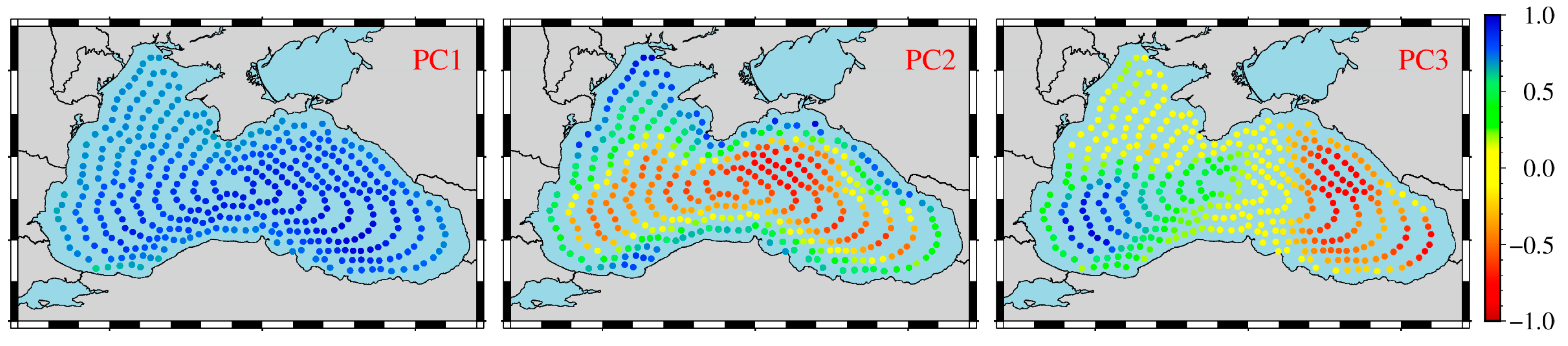
Since 1993, SA has been extensively utilized for monitoring global sea level changes [10,45,46]. To investigate the effects of coastal proximity and spatial heterogeneity on regional sea level estimation, this study employs a virtual altimetry station methodology [47]; a ring of stations positioned along the outer margin of the Black Sea coastline, then incrementally extended inward toward the basin’s interior until the entire sea area was adequately covered. Ultimately, a total of 406 virtual altimetry stations were identified for analysis (Figure 1).

Previous studies have demonstrated that SA observations are affected by various types of noise, which can degrade the precision of sea level trend estimations and increase the uncertainty in estimates of sea level change [48,49]. To mitigate the impact of such noise and more accurately extract long-term trends, this study employed four noise models—ARFIMA (1, d, 1), ARMA (1, 1), GGM, and WN. The characteristics of sea level change for each time period were determined based on the optimal model selected according to the BIC_tp with Hector software version 2.1 [50].

Table 1. Sea level trend and uncertainty at representative virtual altimetry stations under different noise models.

Noise Model	Station 001 (mm/yr)		Station 011 (mm/yr)		Station 122 (mm/yr)
	Trend	Uncertainty	Trend	Uncertainty	Trend	Uncertainty
ARFIMA (1, d, 1)	2.57	1.81	2.39	1.54	2.68	2.25
ARMA (1, 1)	2.10	0.42	1.99	0.46	2.10	0.45
GGM	2.10	0.28	2.00	0.26	2.11	0.56
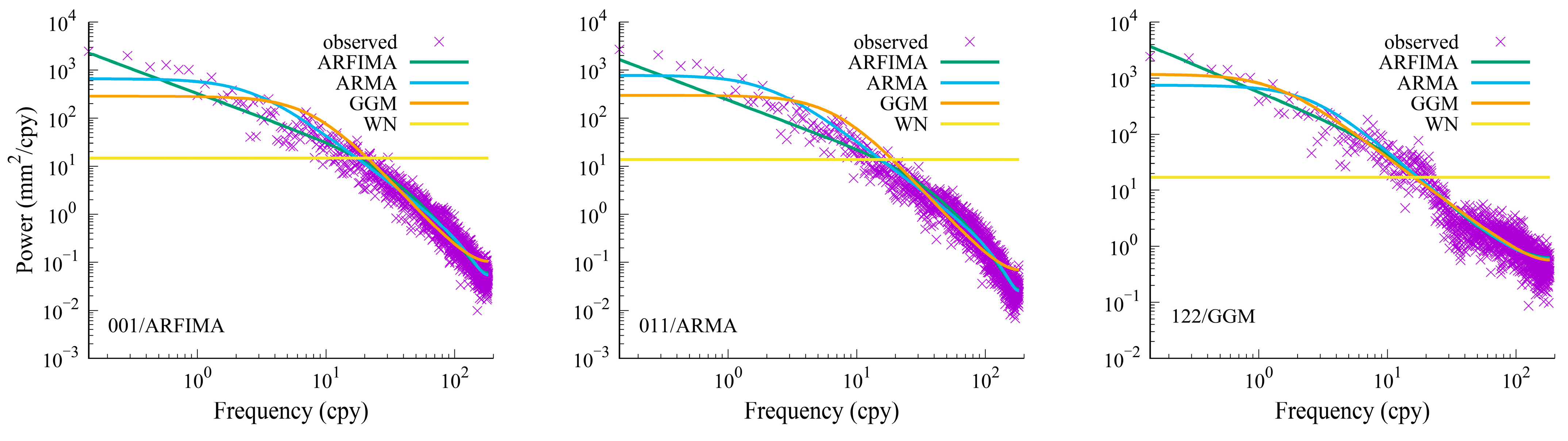
WN	2.09	0.06	2.00	0.06	2.07	0.07

illustrates representative stations selected under the optimal noise models based on the BIC_tp criterion (001/ARFIMA; 011/ARMA; 122/GGM), alongside sea level trend estimates and their associated uncertainties derived from four different noise models.

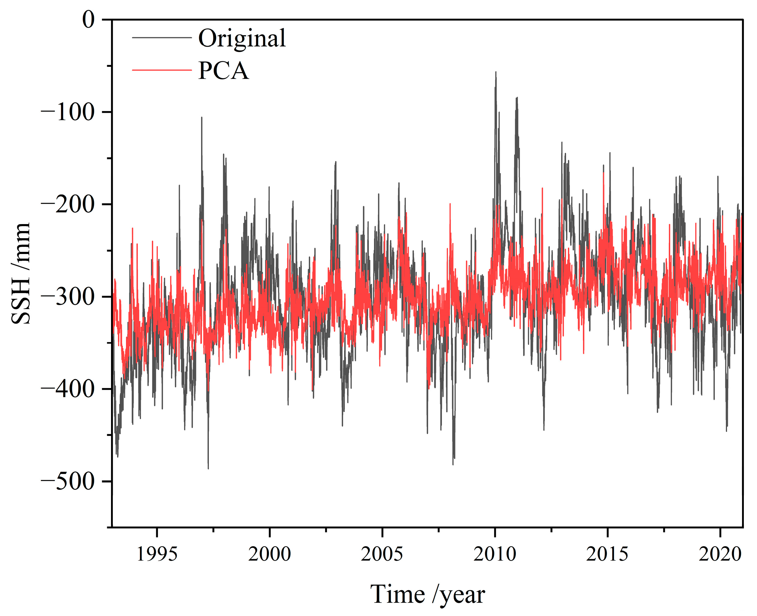
Under different noise models, long-term sea level trend estimates exhibit significant variation. These results highlight that neglecting colored noise or applying an inappropriate noise model can introduce systematic biases into trend estimation. Figure 3 presents the power spectral densities (PSDs) of the SSH residuals at stations 001, 011, and 122, obtained under four different noise models. The PSDs provide a frequency perspective, enabling a visual assessment of each model’s ability to fit the observed data and evaluate whether the noise structure within the time series is adequately captured.

The PSDs of sea level residuals under different stochastic models highlight the presence of colored noise in sea level time series and reveal variations in model performance across stations. These findings underscore the importance of selecting an appropriate noise model to ensure reliable trend estimation and accurate uncertainty quantification. Previous studies have also demonstrated that the duration of the observational time series exerts a substantial influence on the accuracy of sea level trend estimations [51]. To investigate the temporal evolution of sea level in the Black Sea and evaluate the effect of time period on trend estimation, sea level change and their associated uncertainties were estimated for eight different time periods. To assess the robustness of the results, the derived sea level trends were compared with those reported in the previous literature over comparable periods, and both consistencies and discrepancies were examined (

Table 2. Sea level trends in the Black Sea across different time periods, as estimated under the optimal noise model (the number after the ± sign represents the standard deviation in this work).

This Work		Existed Research
Time Span (Year)	Trend (mm/yr)	Authors	Results (mm/yr)	Time Span (Year)
1993–2000	21.68 ± 4.05	Cazenave et al. [52]	27.3 ± 2.50	1993–1998
1993–2003	10.61 ± 1.61	-	-	-
1993–2005	8.84 ± 1.62	Kubryakov et al. [20]	7.60 ± 0.30	1993–2005
1993–2008	3.68 ± 0.89	-	-	-
1993–2011	6.74 ± 0.83	-	-	-
1993–2013	4.14 ± 0.69	Kubryakov et al. [25]	3.15 ± 0.13	1993–2014
1993–2017	3.07 ± 0.61	Avsar et al. [53]	2.50 ± 0.50	1993–2017
1993–2020	2.34 ± 0.59	CMEMS	1.40 ± 0.83	1993–2022
1993–2020PCA	1. 76 ± 0.56

).

The results of this study indicate that the Black Sea experienced a significant upward trend in sea level during 1993–2000, with an estimated trend of 21.68 ± 4.05 mm/yr. This finding is consistent with a previous study based on CNES/AVISO satellite altimetry data, which reported a trend of 27.30 ± 2.50 mm/yr for 1993–1998 [52]. Cazenave et al. pointed out that the abnormal sea level rise during this period may be driven by multiple factors, including the expansion of the surface water body due to heating and the reduction of the runoff of major rivers into the sea, which led to a positive water balance and weakened the seasonal sea level fluctuations.

This study shows that the sea level trend in the Black Sea during 1993–2005 was 8.84 ± 1.62 mm/yr, which is consistent within the uncertainty range with the estimate of 7.6 ± 0.3 mm/yr reported by Kubryakov [20] based on tide gauge records and satellite altimetry data from the Division for Space Oceanography of Collecte Localisation Satellites, and this elevated rate has been attributed to decadal-scale variability and the spatially non-uniform nature of sea level changes in the region.

During the period 1993–2013, the sea level trend in the Black Sea was estimated in this study to be 4.14 ± 0.69 mm/yr. This estimate is in reasonable agreement with the result reported by a previous study [25], which derived a rate of 3.15 ± 0.13 mm/yr for the period 1993–2014 using daily sea level anomaly data from AVISO altimetry. Kubryakov et al. indicated that variations in the mean sea level of the Black Sea are primarily governed by its water balance. Moreover, the observed spatial heterogeneity in sea level is closely linked to the basin’s internal dynamical processes.

This study estimated a sea level rise rate of 3.07 ± 0.61 mm/yr in the Black Sea during the period 1993–2017. Avsar and Kutoğlu [53], based on daily SSH data provided by CMEMS, estimated the mean sea level rise in the Black Sea to be 2.50 ± 0.50 mm/yr after removing seasonal cycles from the SSH time series. The study also highlighted the significant interannual variability in the non-seasonal sea level changes in the Black Sea.

The estimated sea level trend in this study is 2.34 ± 0.59 mm/yr for 1993–2020, and CMEMS reported a sea level trend of 1.40 ± 0.83 mm/yr in the Black Sea, based on the OMI_CLIMATE_SL_BLKSEA_area_averaged_anomalies product (https://doi.org/10.48670/moi-00215, accessed on 7 October 2024). The CMEMS estimate was corrected for TOPEX-A instrumental drift and basin-averaged glacial isostatic adjustment (GIA), and further processed by removing seasonal, annual, and semi-annual signals, followed by low-pass filtering to isolate long-term trends.

A comparative analysis reveals that the characteristics of sea level change exhibit temporal variability across different periods. During the same time period, our estimates generally align with those reported in existing studies, although some discrepancies are evident. These differences may be attributed to variations in the SA data products and the methods used for station selection. For instance, Kubryakov and Stanichnyi [20] utilized a dataset specifically tailored for the Black Sea, characterized by a temporal resolution of 10 days and a spatial resolution of 7 km, to estimate sea level trend over 1993–2005, based on station data located along satellite altimetry tracks. Kubryakov et al. [25] used regional grid data of sea level anomalies to estimate sea level change over the period 1993–2014. The sea level trend data for the Black Sea provided by CMEMS during 1993–2022 are based on a dedicated satellite altimetry dataset for the Black Sea and account for the effects of GIA. In general, sea level change in the Black Sea does not follow a strictly linear pattern. While the long-term trend indicates an upward trajectory, the rate of change exhibits variability across different time periods. During the period 1993–2000, the sea level trend was as high as 21.68 mm/yr, but this trend slowed afterward, with the rate of change fluctuating between 2 and 8 mm/yr after 2005.

3.2. Analysis of Sea Level Trend Uncertainty in the Black Sea

To evaluate the impact of time series length on the accuracy of sea level trend estimation, this study investigates the uncertainties in sea level trend across eight distinct time periods (

Table 3. Uncertainties of sea level trend in the Black Sea under the optimal noise model across different time periods (1993–2020_dnoise reflects the uncertainty in the estimated sea level trend following the application of PCA-based denoising).

Time Span (Year)	Uncertainty (mm/yr)
1993–2000	12.41
1993–2003	8.70
1993–2005	7.16
1993–2008	5.72
1993–2011	5.07
1993–2013	4.57
1993–2017	3.75
1993–2020	3.20
1993–2020dnoise	1.27

). By analyzing trend estimates derived from time series spanning short (1993–2000) to extended (1993–2020) periods, this study highlights the sensitivity of trend calculations to the length of the observational record and provides a detailed assessment of the robustness and reliability of trend detection in the Black Sea.

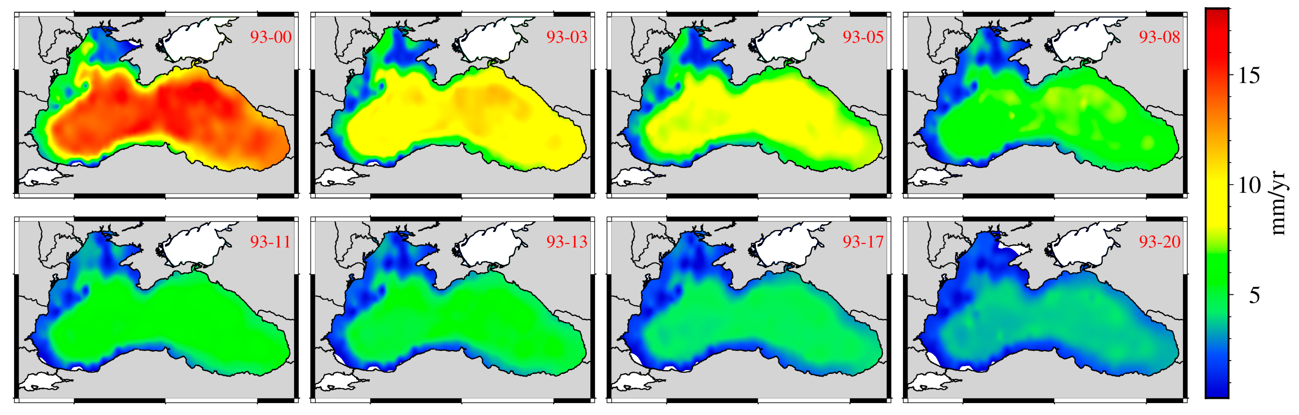
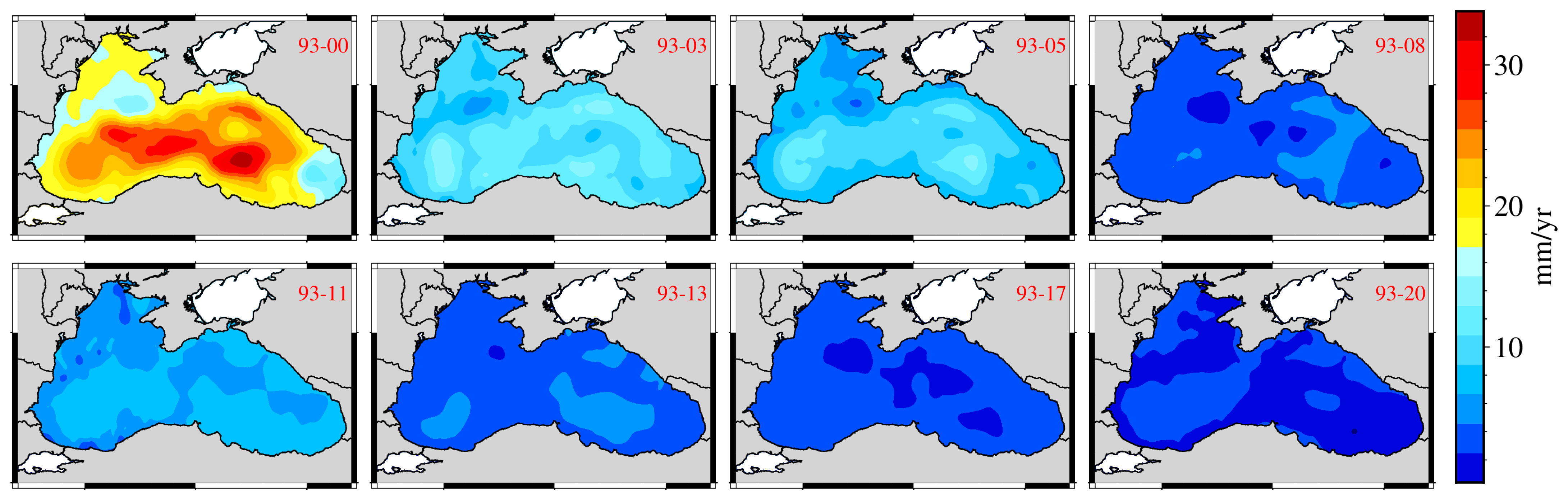
The uncertainty of the trend is influenced by both the duration of the observational time series and the presence of noise, with its magnitude serving as an indicator of the stability and reliability of the estimated trend. Figure 4 shows the spatial variability in the trend of uncertainty over different periods.

It can be observed from Figure 4 that the uncertainty of sea level trend estimation for the Black Sea gradually decreases with increasing time span (7, 10, 12, 15, 18, 20, 24, and 28 years). Sea level variability in the Black Sea is thought to be influenced by both large-scale and mesoscale dynamical processes. In particular, the deep-water regions are characterized by more complex oceanic dynamics, including mesoscale eddies and deep circulation. These processes are likely to introduce significant spatial and temporal variability in SSH, which may in turn contribute to regional differences in sea level trends and to the comparatively higher uncertainty observed in the central basin. Further research is needed to fully understand the mechanisms responsible for these uncertainties.

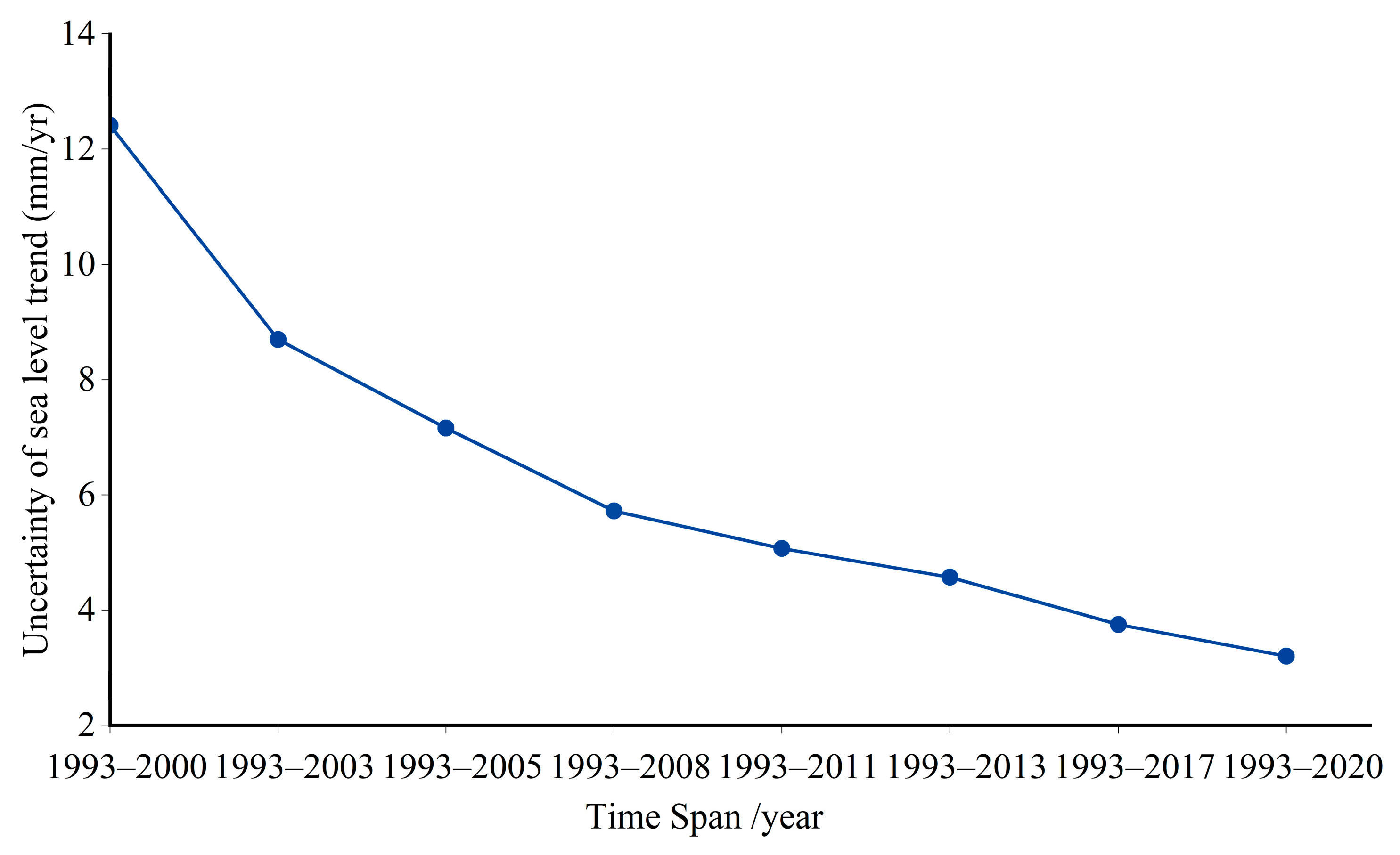
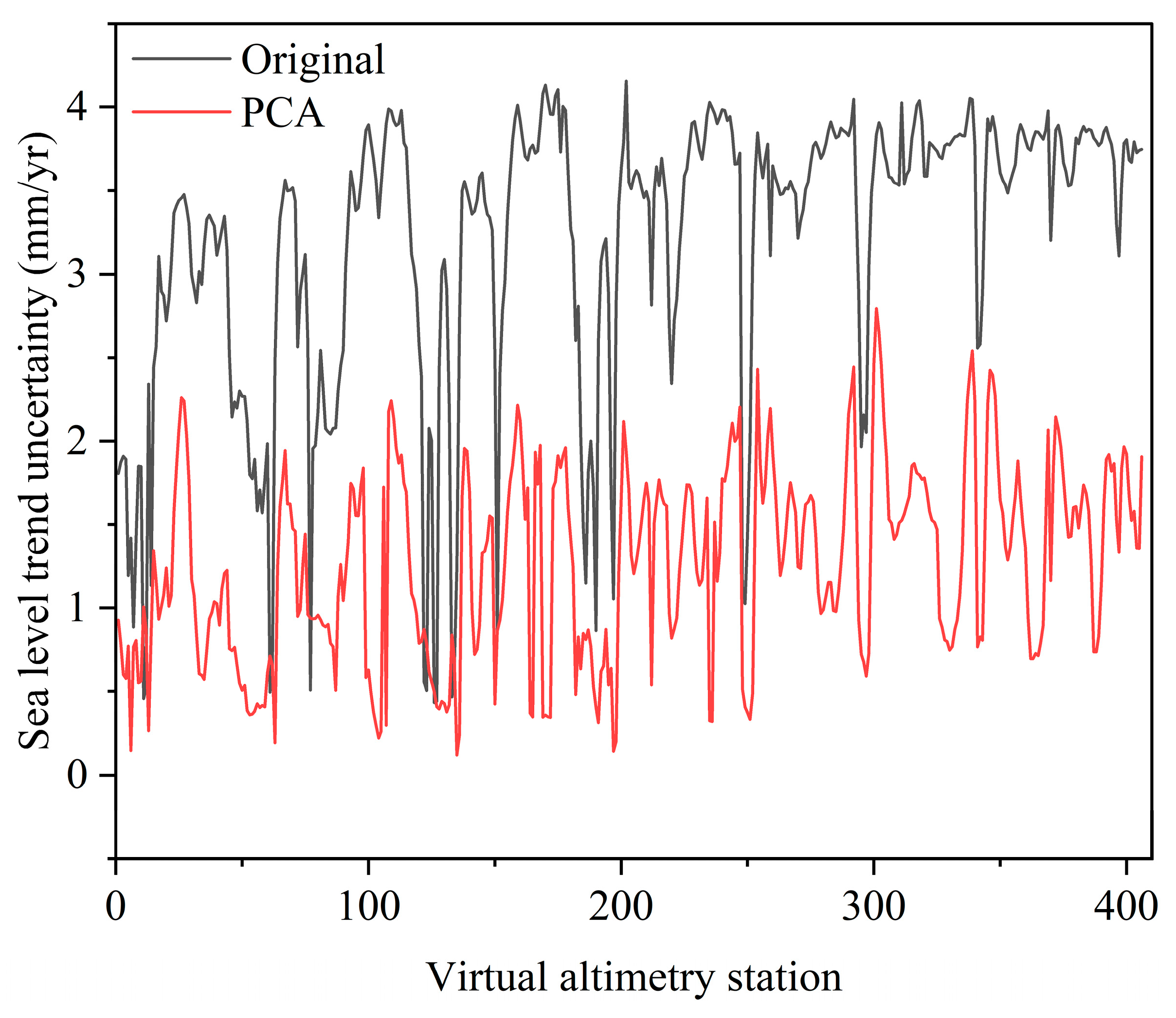
The uncertainty of sea level trend estimation exhibits a clear time-dependent behavior, decreasing progressively with the extension of the observation period (Figure 5). For the period 1993–2000, the uncertainty in sea level trend estimates reaches 12.41 mm/yr, whereas it substantially reduces to 3.20 mm/yr over the 1993–2020 interval. This uncertainty decline follows a non-linear decay pattern: within the first 15 years (1993–2008), it drops by 54% (from 12.41 mm/yr to 5.72 mm/yr), while achieving similar improvements in precision over subsequent decades requires increasingly longer observation records. This is largely due to the high sensitivity of sea level trends to interannual and decadal variability, which limits the ability of short-term records to distinguish long-term signals from short-term fluctuations, thereby amplifying trend uncertainty [48].

In the semi-enclosed Black Sea, sea level variability is further influenced by regional climate conditions and ocean circulation. Short time series may fail to capture the full range of such variability, and reliance on a limited number of SA observations can introduce substantial uncertainty in trend estimation [20]. In contrast, long-term time series are more effective in identifying interannual and decadal variability and isolating the long-term trend through improved noise reduction, resulting in more robust and reliable estimates [54]. By analyzing sea level trends and their associated uncertainties across different temporal scales, our results demonstrate that the uncertainty of the estimated sea level trend decreases notably with increasing observational period. Over the 28-year period from 1993 to 2020, the uncertainty is approximately 3.20 mm/yr, indicating a substantial improvement in trend stability compared to shorter periods. Based on our results, we recommend using time series longer than 28 years to enhance the robustness and accuracy of sea level trend estimation.

3.3. Spatial Variation of Sea Level Trend in the Black Sea

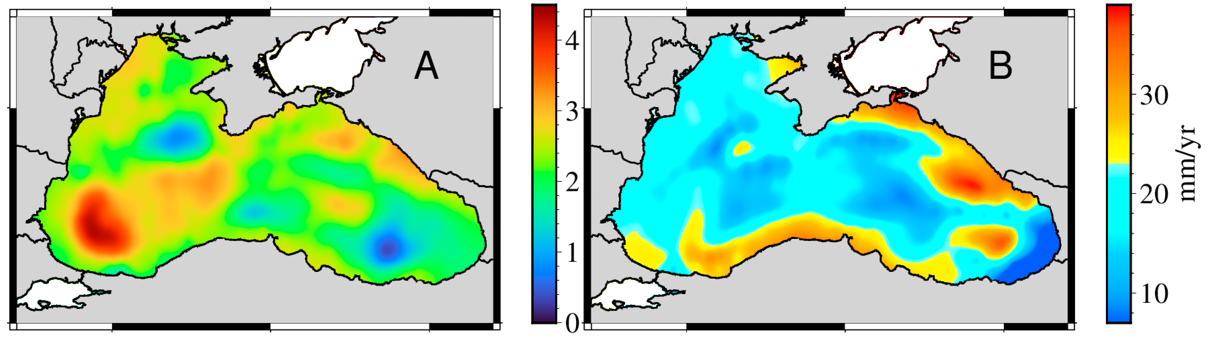
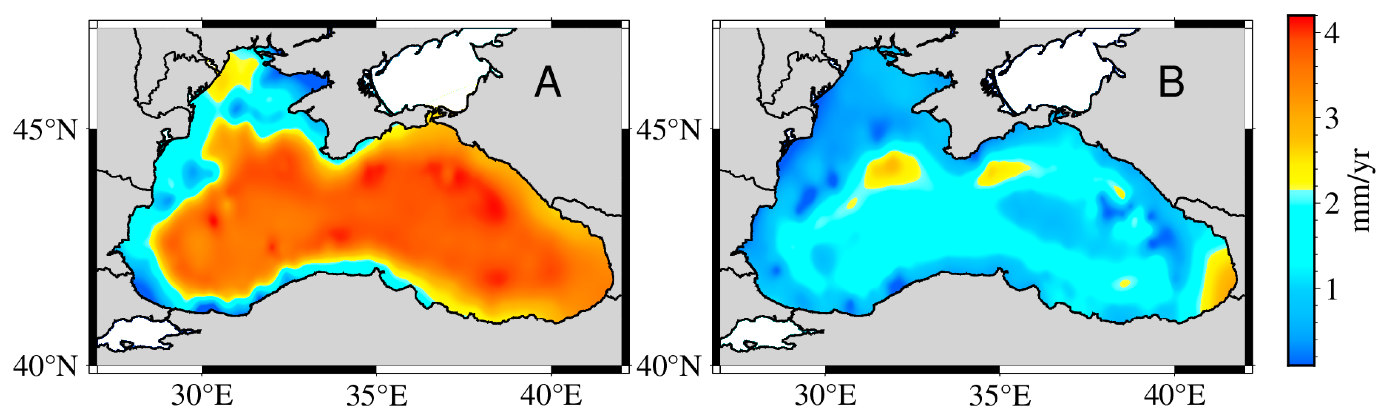
To further investigate the spatial distribution characteristics of sea level change in the Black Sea, this study utilizes SA data spanning the period 1993–2020, using sea level trends estimated from 406 virtual altimetry stations under their respective optimal noise models, a spatial distribution map of sea level trends in the Black Sea region was generated through geospatial interpolation techniques (Figure 6A).

Figure 6A shows the spatial variation of mean sea level trends in the Black Sea from 1993 to 2020, with an average basin-wide trend of approximately 2.34 mm/yr. Long-term changes in the dynamic regime of the Black Sea have a significant impact on the spatial variability of sea level trends [25]. Previous studies have identified water balance as the dominant driver of long-term sea level change in the Black Sea [55]. Along the western coast, inflows from major rivers such as the Danube and Dnieper affect local sea levels, primarily through variations in river discharge. The maximum sea level trend of 4.22 mm/yr is observed in the southwestern sector of the basin, adjacent to the Turkish Straits, highlighting the region’s vulnerability to climate-induced hydrological changes. This region is subject to dynamic influences from water exchange through the straits and is modulated by the topographic constraints of the continental shelf; strong wind events can alter the net flow through the straits, subsequently impacting sea level [56]. Furthermore, studies have shown that the highest average significant wave heights also occur in this southwestern zone near the Turkish coast [57], indicating that the sea level change in this area is more significant due to the influence of dynamic factors. In contrast, the southeastern Black Sea displays a lower sea level trend compared to other regions, which may be associated with the presence of anticyclonic gyres. Cyclonic and anticyclonic gyres can induce regional water accumulation or depletion, thereby modulating sea level variability in the area [58].

3.4. Seasonal Change in the Black Sea

Due to localized oceanographic processes, sea level changes across different regions of the Black Sea basin exhibit marked spatial heterogeneity. In semi-enclosed basins such as the Black Sea, sea level variability is neither temporally linear nor spatially uniform [59]. Sea level changes are influenced not only by long-term trends but also by short-term variability, including seasonal climatic fluctuations, ocean circulation patterns, wind stress, and thermohaline structure [60]. This study investigates the characteristics of seasonal variability in the Black Sea by analyzing annual amplitude across eight different time periods. According to the statistical results (

Table 4. Temporal evolution of annual sea level amplitude in the Black Sea across eight time periods.

Time Span (Year)	Annual Amplitude (mm)	Uncertainty (mm)
1993–2000	26.45	10.57
1993–2003	22.95	8.83
1993–2005	24.22	8.30
1993–2008	21.08	7.32
1993–2011	21.45	7.13
1993–2013	21.74	6.90
1993–2017	20.06	6.18
1993–2020	19.23	5.69
1993–2020PCA	14.74	2.68

), the annual amplitudes remain relatively stable over time, with only minor fluctuations between intervals. A slight decreasing trend in amplitude is observed with increasing temporal coverage, which may be associated with evolving climate patterns, adjustments in ocean circulation, or interannual variability.

To further explore the spatial characteristics of seasonal oscillations, a spatial distribution map of annual amplitudes for the period 1993–2020 was generated (Figure 6B), highlighting regional disparities in seasonal sea level variability across the basin.

The annual amplitude of sea level variation of the Black Sea is not uniformly distributed. Higher amplitudes are observed along the northeastern and southern coasts compared to the central basin. This spatial pattern may be attributed to the cyclonic boundary currents and basin-scale dynamics, which tend to elevate coastal sea levels [61,62]. Seasonal amplitude is further enhanced by local storm surges and Ekman transport, both of which are influenced by prevailing wind patterns [25]. In contrast, the interior basin, constrained by the semi-enclosed nature of the Black Sea, exhibits relatively lower amplitudes. Seasonal sea level variations are modulated by multiple factors, including atmospheric pressure fluctuations, wind stress, river discharge, water balance, and oceanic dynamics. To further investigate the characteristics of seasonal variability and the timing of sea level maxima, this study analyzed SA-derived SSH time series at 406 virtual altimetry stations over the 28-year period from 1993 to 2020, identifying the months in which peak sea levels occur. For each station, we extracted the month corresponding to the maximum SSH value in each year, and obtained a total of 28 “maximum months”. Then, we counted the number of times each Gregorian calendar month (January to December) was marked as the “month of maximum sea level height “ in all stations and years, and finally obtained the frequency of the maximum sea level in the year corresponding to each month (

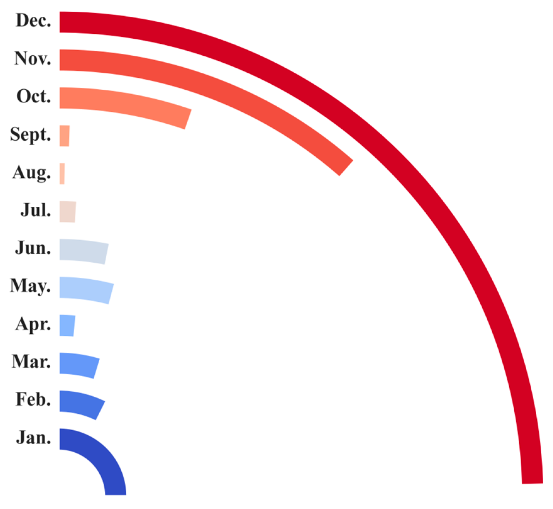
Table 5. Month of maximum sea level height at 406 virtual altimetry stations over the period 1993–2020.

Month	Stations Count	Percentage (%)
January	3190	28.06
February	942	8.28
March	600	5.28
April	195	1.72
May	524	4.61
June	404	3.55
July	125	1.10
August	41	0.36
September	64	0.56
October	676	5.95
November	1466	12.90
December	3141	27.63

).

Statistical analysis reveals that peak sea levels at most stations occur predominantly in December and January, comprising 27.63% and 28.06% of occurrences, respectively (Figure 7). This seasonal pattern aligns with the dynamics of freshwater inflow, as the Black Sea basin typically experiences the highest precipitation during the winter months, coupled with peak river discharge in the spring. The combined effects of increased winter precipitation and intensified river inflow during spring likely contribute to elevated sea levels observed in December and January. Aydın and Beşiktepe [63] reported that the highest sea levels generally occur between spring and summer, while the lowest levels are observed during autumn when river discharge is minimal. Sea level variability in the Black Sea has also been shown to be influenced by the North Atlantic Oscillation (NAO), which regulates terrestrial water storage and indirectly contributes to sea level fluctuations [23,64]. Sea level fluctuations in the Black Sea exhibit a negative correlation with the NAO index, with elevated sea levels typically occurring during negative NAO phases [65]. During these phases, increased precipitation and river runoff enhance freshwater input into the basin, while intensified wind forcing can reduce outflow through the Bosphorus Strait, further amplifying sea level rise.

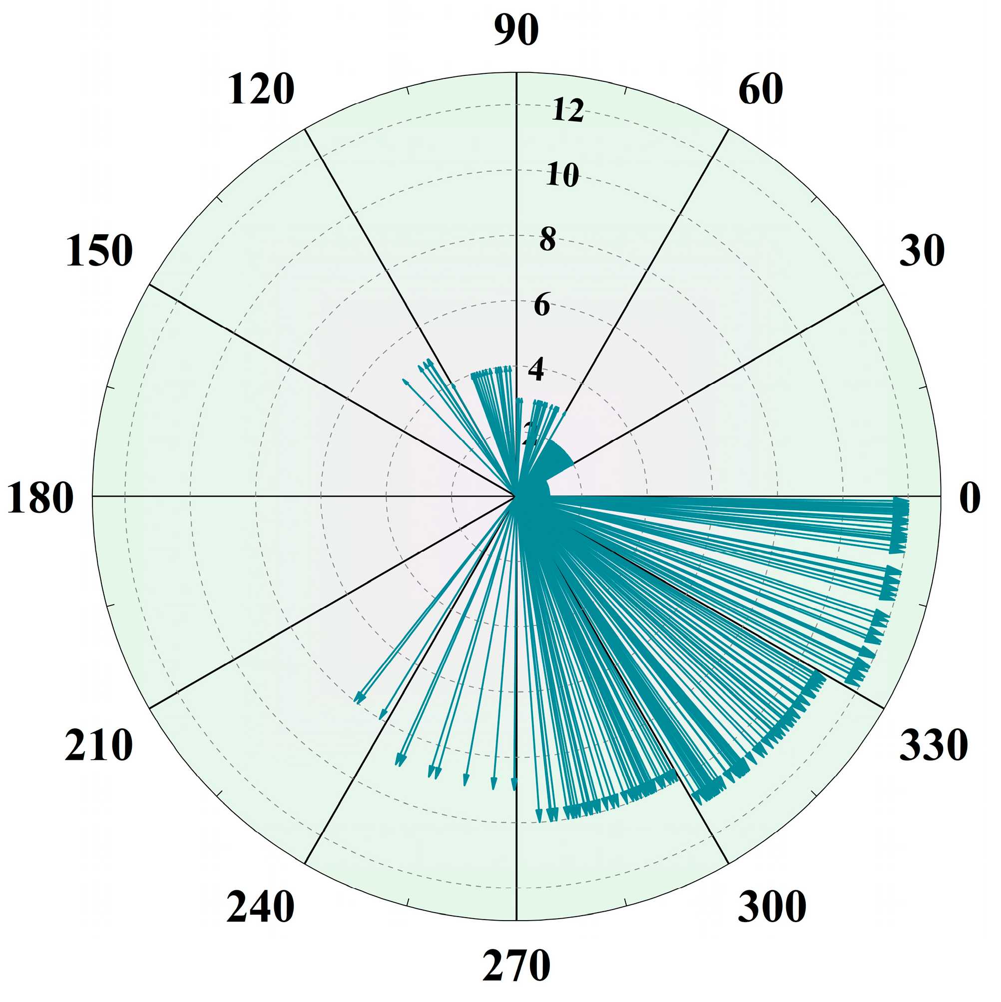
To investigate the spatiotemporal characteristics, dynamic evolution, and seasonal patterns of the annual amplitude of sea level variability in the Black Sea, this study analyzes the phase values derived from 406 virtual altimetry stations for the period 1993–2020. To identify the calendar month associated with the peak of the annual cycle, the phase angle is first normalized over the full 360-degree annual period and then linearly mapped onto a 12-month calendar scale, with 30 degrees representing one month. Statistical analysis identifies the calendar month corresponding to the maximum annual amplitude at each station (

Table 6. Maximum annual amplitude occurrence month for 406 virtual altimetry stations in the Black Sea over the period 1993–2020.

Month	Stations Count	Percentage (%)
January	117	28.82
February	89	21.92
March	18	4.43
April	17	4.19
May	5	1.23
June	0	0.00
July	0	0.00
August	3	0.74
September	8	1.97
October	40	9.85
November	62	15.27
December	47	11.58

), revealing the temporal distribution pattern of peak annual sea level variability across the Black Sea.

Table 6 summarizes the distribution of months in which the maximum annual amplitude of sea level occurs at 406 virtual altimetry stations across the Black Sea from 1993 to 2020. The results reveal a pronounced seasonal pattern, with peak amplitudes predominantly occurring between November and February (Figure 8). Specifically, January and February together account for nearly 51% of all stations (28.82% and 21.92%, respectively), while secondary peaks are observed in November (15.27%) and December (11.58%). In contrast, the number of stations exhibiting peak amplitudes during the summer months (June to August) is negligible. No stations reach their maximum in June or July, and only 0.74% do so in August. This suggests that winter-driven processes dominate in shaping the annual cycle of sea level.

4. Discussion

SA has provided a reliable means of detecting sea level changes since the early 1990s. However, when the observational period is relatively short, it becomes difficult to directly distinguish regional sea level changes associated with climate change from those associated with natural climate variability [66]. To assess the influence of time series length on sea level change, we analyzed the spatial characteristics of sea level trend in the Black Sea over eight different periods. The results reveal notable differences in the trend patterns across these periods, underscoring the non-stationary and regionally heterogeneous nature of sea level change within the basin (Figure 9).

During the period 1993–2000, the Black Sea exhibited relatively large fluctuations in sea level trends. After 2005, the sea level trend exhibited a decline. Previous studies have indicated that sea level variations in this region are closely linked to the discharge of the Danube River during the same period [15]. In contrast, the trend observed over the longer intervals of 1993–2013, 1993–2017, and 1993–2020 displays a more stable pattern, further reinforcing the conclusion that longer time series provide more reliable and consistent estimates of sea level trends. Since sea level estimation is often influenced by noise interference, regional variability, and measurement uncertainties, the SSH time series derived from SA data typically contain colored noise, which compromises the accuracy of the estimates [67]. Seasonal changes in sea level will also affect the accurate estimation of sea level trend; short time series estimation, especially, is more affected. To improve the accuracy of sea level change estimation in the Black Sea, this study applies PCA to denoise the SSH time series over the period 1993–2020. Figure 10 provides an example of virtual altimetry Station 001, illustrating the differences in the sea surface height SSH time series before and after denoising, which demonstrates the effectiveness of the noise reduction method.

As illustrated in the time series plots (Figure 10), the SSH data subjected to PCA-based denoising exhibit a smoother temporal evolution with diminished short-term variability, thereby facilitating a more robust identification of long-term sea level trend. The denoised time series were subsequently utilized to estimate the sea level trend over the Black Sea. To evaluate the impact of PCA-based denoising on trend estimation, we constructed spatial distribution maps of sea level trend for the period 1993–2020 (Figure 11), along with a station comparison of trend estimates before and after denoising (Figure 12).

Figure 11 illustrates the spatial distribution of sea level trends in the Black Sea during the period 1993–2020. After denoising, the sea level trend retains the original spatial characteristics, indicating that the application of PCA effectively attenuates localized noise while preserving the main component of the trend. The resulting spatial pattern shows improved consistency with previously published estimates, reinforcing the robustness and reliability of the trend assessment.

To assess the impact of noise reduction on sea level trend estimation, we applied PCA to the original SSH data from 406 virtual altimetry stations. As shown in Figure 12, the denoised results (red) closely follow the original trends (black), with minimal changes in magnitude. This demonstrates that the PCA-based approach effectively reduces noise while maintaining the integrity of the original spatial trend structure.

Accurate estimation of sea level trends depends critically on the stability of long-term signals. To further assess the effectiveness of PCA-based denoising, we investigated its influence on the uncertainty of sea level trend estimates (Figure 13).

Figure 13 shows the spatial distribution of sea level trend uncertainties in the Black Sea over the period 1993–2020. In panel A, the uncertainties exhibit generally high values across much of the basin, particularly in the central region. After PCA denoising (Figure 13B), the uncertainty levels are significantly reduced throughout the basin, highlighting the effectiveness of the method in enhancing the confidence of sea level trend estimates. The denoised results offer a more reliable spatial representation of long-term sea level changes.

As illustrated in Figure 14, the application of PCA-based denoising to the SSH time series substantially reduces the uncertainty associated with sea level trend estimates across the 406 virtual altimetry stations in the Black Sea. Trend uncertainties derived from the original (black) time series are generally higher, often exceeding 3–4 mm/yr at numerous stations. In contrast, the PCA-denoised series (red) exhibits significantly lower uncertainties at the majority of stations. This widespread reduction demonstrates that PCA effectively mitigates noise that can bias trend estimation, while retaining the underlying long-term sea level signal. Consequently, the statistical robustness of the results is notably enhanced.

PCA was applied to denoise the SSH time series at 406 virtual altimetry stations across the Black Sea for the period 1993–2020. The mean sea level trend after PCA processing was 1.76 ± 0.56 mm/yr (Table 2), showing good consistency with the CMEMS reported of 1.40 ± 0.83 mm/yr for the period 1993–2022. After noise reduction, the original temporal and spatial characteristics of the trend are effectively preserved. Notably, the sea level trend uncertainty was reduced to 1.27 mm/yr after noise reduction (Table 3), with 96.8% of the altimetry stations showing a decrease in uncertainty and an average reduction of 1.92 mm/yr. Furthermore, the root means square error of SSH decreased by an average of 5.06 mm after PCA denoising. Additionally, the mean annual amplitude was reduced from 19.23 mm to 14.74 mm, reflecting a 23.35% reduction (Table 4). These confirm that PCA effectively reduces TCN while preserving the underlying trend, thus enhancing the reliability of sea level estimates in the Black Sea.

5. Conclusions

This study explores the temporal and spatial variability of sea level change in the Black Sea using SA data. By examining sea level trends, associated uncertainties, and annual amplitudes under an optimized noise model across multiple time periods, the analysis reveals notable spatial heterogeneity and seasonal patterns. To mitigate the high uncertainty in trend estimates, PCA was employed to denoise the SSH time series.

(1)

The study estimated sea level trend in the Black Sea over eight progressively longer time periods: 1993–2000, 1993–2003, 1993–2005, 1993–2008, 1993–2011, 1993–2013, 1993–2017, and 1993–2020, with corresponding rates of 21.68 ± 4.05 mm/yr, 10.61 ± 1.61 mm/yr, 8.84 ± 1.62 mm/yr, 3.68 ± 0.89 mm/yr, 6.74 ± 0.83 mm/yr, 4.14 ± 0.69 mm/yr, 3.07 ± 0.61 mm/yr, and 2.34 ± 0.59 mm/yr, respectively. The results indicate a consistent decrease in trend uncertainty as the time series length increases. Consequently, it is recommended that time series of at least 28 years be utilized for sea level trend estimation in the Black Sea to improve the accuracy and reliability of the results. Spatial analyses reveal a heterogeneous sea level response across the basin, likely governed by its semi-enclosed configuration, cyclonic boundary currents, and regional climate forcing, all of which jointly modulate the water balance and regional sea level variability.

(2)

An analysis of the phase values from 406 virtual altimetry stations over the period 1993–2020 revealed that the months of peak annual amplitude predominantly occur between November and February, which is consistent with the finding of the maximum sea level height at the virtual altimetry stations. This seasonal peak is primarily driven by increased winter precipitation and cumulative freshwater input, including enhanced spring river runoff.

(3)

After noise reduction, the sea level trend in the Black Sea for the period 1993–2020 was estimated at 1.76 ± 0.56 mm/yr. PCA effectively preserved the original temporal and spatial trend patterns while significantly reducing uncertainty to 1.27 mm/yr (96.8% stations improved) and lowering SSH root mean square error by 5.06 mm. The mean annual amplitude decreased by 23.35%, confirming that PCA efficiently removes noise and enhances the accuracy of sea level trend estimates.

Although this study evaluates sea level trends in the Black Sea using virtual altimetry stations, several limitations remain. The analysis primarily relies on SA data, and future research would benefit from integrating multi-source observations to enhance robustness and accuracy. PCA effectively reduces trend uncertainty, but as a linear method, it may fail to fully capture non-linear features or abrupt changes in the SSH time series. Moreover, sea level variability in the Black Sea is strongly influenced by regional atmospheric forcing; future studies should integrate climate indices and wind stress data to further investigate the mechanisms driving sea level changes in this semi-enclosed basin. With ongoing improvements in the temporal resolution and accuracy of SA missions, finer-scale and previously unresolved spatiotemporal sea level variations are expected to become increasingly accessible. Building on these perspectives, future research will focus on the physical drivers of sea level change in the Black Sea through multi-scale decomposition and modal analysis of sea level time series. Physics-informed neural networks and other AI techniques will be incorporated to identify key dynamic factors and internal couplings by integrating data-driven methods with physical constraints [68,69,70]. This integrated framework—combining data processing, signal decomposition, and physical modeling—is expected to improve understanding of sea level variability and support regional environmental assessments and early warning efforts.

References

1. Stammer, D.; Cazenave, A.; Ponte, R.M.; Tamisiea, M.E. Causes for contemporary regional sea level changes. Annu. Rev. Mar. Sci. 2013, 5, 21–46. [Google Scholar] [CrossRef] [PubMed]
2. Carson, M.; Köhl, A.; Stammer, D.; A. Slangen, A.B.; Kat sman, C.A.; van de Wal, R.S.W.; Church, J.; White, N. Coastal sea level changes, observed and projected during the 20th and 21st century. Clim. Change 2016, 134, 269–281. [Google Scholar] [CrossRef]
3. Huang, J.; Feng, W.; Yang, Y.; Xiong, Y.; Yang, M.; Zhong, M. Significant impact of non-tidal oceanic and atmospheric mass variations on regional ocean mass budgets: A comparative analysis across 19 representative regions. J. Geophys. Res. Ocean. 2025, 130, e2024JC021477. [Google Scholar] [CrossRef]
4. Griggs, D.J.; Noguer, M. Climate change 2001: The scientific basis. Contribution of working group I to the third assessment report of the intergovernmental panel on climate change. Weather 2002, 57, 267–269. [Google Scholar] [CrossRef]
5. Dasgupta, S.; Laplante, B.; Meisner, C.; Wheeler, D.; Yan, J. The impact of sea level rise on developing countries: A comparative analysis. Clim. Change 2009, 93, 379–388. [Google Scholar] [CrossRef]
6. Nerem, R.S.; Chambers, D.P.; Choe, C.; Mitchum, G.T. Estimating mean sea level change from the TOPEX and Jason altimeter missions. Mar. Geod. 2010, 33, 435–446. [Google Scholar] [CrossRef]
7. Roy, P.; Pal, S.C.; Chakrabortty, R.; Chowdhuri, I.; Saha, A.; Shit, M. Effects of climate change and sea-level rise on coastal habitat: Vulnerability assessment, adaptation strategies and policy recommendations. J. Environ. Manag. 2023, 330, 117187. [Google Scholar] [CrossRef]
8. Church, J.A.; White, N.J. Sea-level rise from the late 19th to the early 21st century. Surv. Geophys. 2011, 32, 585–602. [Google Scholar] [CrossRef]
9. Ablain, M.; Legeais, J.F.; Prandi, P.; Marcos, M.; Fenoglio-Marc, L.; Dieng, H.B.; Benveniste, J.; Cazenave, A. Satellite Altimetry-based Sea Level at Global and Regional Scales. In Integrative Study of the Mean Sea Level and Its Components; Springer International Publishing: Cham, Switzerland, 2017; pp. 9–33. [Google Scholar]
10. Cazenave, A.; Moreira, L. Contemporary sea-level changes from global to local scales: A review. Proc. R. Soc. A 2022, 478, 20220049. [Google Scholar] [CrossRef]
11. Nicholls, R.J.; Lincke, D.; Hinkel, J.; Brown, S.; Vafeidis, A.T.; Meyssignac, B.; Hanson, S.E.; Merkens, J.-L.; Fang, J. A global analysis of subsidence, relative sea-level change and coastal flood exposure. Nat. Clim. Change 2021, 11, 338–342. [Google Scholar] [CrossRef]
12. Khojasteh, D.; Glamore, W.; Heimhuber, V.; Felder, S. Sea level rise impacts on estuarine dynamics: A review. Sci. Total Environ. 2021, 780, 146470. [Google Scholar] [CrossRef]
13. Poulos, S.E. The Mediterranean and Black Sea Marine System: An overview of its physico-geographic and oceanographic characteristics. Earth-Sci. Rev. 2020, 200, 103004. [Google Scholar] [CrossRef]
14. Bakan, G.; Büyükgüngör, H. The black sea. Mar. Pollut. Bull. 2000, 41, 24–43. [Google Scholar] [CrossRef]
15. Kostianoy, A.G.; Kosarev, A.N. (Eds.) The Black Sea Environment. In The Handbook of Environmental Chemistry; Springer: Berlin/Heidelberg, Germany, 2008; 457p. [Google Scholar]
16. Demirkesen, A.C.; Evrendilek, F.; Berberoglu, S. Quantifying coastal inundation vulnerability of Turkey to sea-level rise. Environ. Monit. Assess. 2008, 138, 101–106. [Google Scholar] [CrossRef] [PubMed]
17. Görmüş, T.; Ayat, B.; Aydoğan, B.; Tătui, F. Basin scale spatiotemporal analysis of shoreline change in the Black Sea. Estuar. Coast. Shelf Sci. 2021, 252, 107247. [Google Scholar] [CrossRef]
18. Stanev, E.V.; Peneva, E.L. Regional sea level response to global climatic change: Black Sea examples. Glob. Planet. Change 2001, 32, 33–47. [Google Scholar] [CrossRef]
19. Korotaev, G.K.; Saenko, O.A.; Koblinsky, C.J. Satellite altimetry observations of the Black Sea level. J. Geophys. Res. Ocean. 2001, 106, 917–933. [Google Scholar] [CrossRef]
20. Kubryakov, A.A.; Stanichnyi, S.V. The Black Sea level trends from tide gages and satellite altimetry. Russ. Meteorol. Hydrol. 2013, 38, 329–333. [Google Scholar] [CrossRef]
21. Avsar, N.B.; Kutoglu, S.H.; Jin, S.; Erol, B. Investigaton of sea level change along the Black Sea coast from tide gauge and satellite altimetry. Int. Arch. Photogramm. Remote Sens. Spat. Inf. Sci. 2015, 40, 67–71. [Google Scholar] [CrossRef]
22. Avsar, N.B.; Jin, S.; Kutoglu, H.; Gurbuz, G. Sea level change along the Black Sea coast from satellite altimetry, tide gauge and GPS observations. Geod. Geodyn. 2016, 7, 50–55. [Google Scholar] [CrossRef]
23. Volkov, D.L.; Landerer, F.W. Internal and external forcing of sea level variability in the Black Sea. Clim. Dyn. 2015, 45, 2633–2646. [Google Scholar] [CrossRef]
24. Volkov, D.L.; Johns, W.E.; Belonenko, T.V. Dynamic response of the Black Sea elevation to intraseasonal fluctuations of the Mediterranean sea level. Geophys. Res. Lett. 2016, 43, 283–290. [Google Scholar] [CrossRef]
25. Kubryakov, A.A.; Stanichny, S.V.; Volkov, D.L. Quantifying the impact of basin dynamics on the regional sea level rise in the Black Sea. Ocean Sci. 2017, 13, 443–452. [Google Scholar] [CrossRef]
26. Causio, S.; Federico, I.; Jansen, E.; Mentaschi, L.; Ciliberti, S.A.; Coppini, G.; Lionello, P. The Black Sea near-past wave climate and its variability: A hindcast study. Front. Mar. Sci. 2024, 11, 1406855. [Google Scholar] [CrossRef]
27. Law-Chune, S.; Aouf, L.; Dalphinet, A.; Levier, B.; Drillet, Y.; Drevillon, M. WAVERYS: A CMEMS global wave reanalysis during the altimetry period. Ocean Dyn. 2021, 71, 357–378. [Google Scholar] [CrossRef]
28. Sun, X.; Lu, T.; Wang, Z. Comparative Analysis of Different Deep Learning Algorithms for the Prediction of Marine Environmental Parameters Based on Cmems Products. Acta Geodyn. Geomater. 2024, 21, 343–363. [Google Scholar] [CrossRef]
29. Granger, C.W.; Joyeux, R. An introduction to long-memory time series models and fractional differencing. J. Time Ser. Anal. 1980, 1, 15–29. [Google Scholar] [CrossRef]
30. Beran, J. Maximum likelihood estimation of the differencing parameter for invertible short and long memory autoregressive integrated moving average models. J. R. Stat. Soc. Ser. B (Methodol.) 1995, 57, 659–672. [Google Scholar] [CrossRef]
31. Sowell, F. Maximum likelihood estimation of stationary univariate fractionally integrated time series models. J. Econom. 1992, 53, 165–188. [Google Scholar] [CrossRef]
32. Shumway, R.H.; Stoffer, D.S.; Stoffer, D.S. Time Series Analysis and Its Applications; Springer: Berlin/Heidelberg, Germany, 2000; Volume 3. [Google Scholar]
33. Feng, X.; Schulteis, J. Identification of high noise time series signals using hybrid ARMA modeling and neural network approach. In Proceedings of the IEEE International Conference on Neural Networks, San Francisco, CA, USA, 28 March–1 April 1993; pp. 1780–1785. [Google Scholar]
34. Harville, D. Extension of the Gauss-Markov theorem to include the estimation of random effects. Ann. Stat. 1976, 4, 384–395. [Google Scholar] [CrossRef]
35. Williams, S. The effect of coloured noise on the uncertainties of rates estimated from geodetic time series. J. Geod. 2003, 76, 483–494. [Google Scholar] [CrossRef]
36. Langbein, J. Noise in two-color electronic distance meter measurements revisited. J. Geophys. Res. Solid Earth 2004, 109, B04406. [Google Scholar] [CrossRef]
37. Moffat, I.U.; Akpan, E.A. White noise analysis: A measure of time series model adequacy. Appl. Math. 2019, 10, 989–1003. [Google Scholar] [CrossRef]
38. Roweis, S. EM algorithms for PCA and SPCA. Adv. Neural Inf. Process. Syst. 1997, 626–632. [Google Scholar]
39. Ringnér, M. What is principal component analysis? Nat. Biotechnol. 2008, 26, 303–304. [Google Scholar] [CrossRef]
40. He, X.; Hua, X.; Yu, K.; Xuan, W.; Lu, T.; Zhang, W.; Chen, X. Accuracy enhancement of GPS time series using principal component analysis and block spatial filtering. Adv. Space Res. 2015, 55, 1316–1327. [Google Scholar] [CrossRef]
41. Abdi, H.; Williams, L.J. Principal component analysis. Wiley Interdiscip. Rev. Comput. Stat. 2010, 2, 433–459. [Google Scholar] [CrossRef]
42. Dong, D.; Fang, P.; Bock, Y.; Webb, F.; Prawirodirdjo, L.; Kedar, S.; Jamason, P. Spatiotemporal filtering using principal component analysis and Karhunen-Loeve expansion approaches for regional GPS network analysis. J. Geophys. Res. Solid Earth 2006, 111, B03405. [Google Scholar] [CrossRef]
43. Greenacre, M.; Groenen, P.J.; Hastie, T.; d’Enza, A.I.; Markos, A.; Tuzhilina, E. Principal component analysis. Nat. Rev. Methods Primers 2022, 2, 100. [Google Scholar] [CrossRef]
44. Maćkiewicz, A.; Ratajczak, W. Principal components analysis (PCA). Comput. Geosci. 1993, 19, 303–342. [Google Scholar] [CrossRef]
45. Guérou, A.; Meyssignac, B.; Prandi, P.; Ablain, M.; Ribes, A.; Bignalet-Cazalet, F. Current observed global mean sea level rise and acceleration estimated from satellite altimetry and the associated measurement uncertainty. Ocean Sci. 2023, 19, 431–451. [Google Scholar] [CrossRef]
46. Adebisi, N.; Balogun, A.-L.; Min, T.H.; Tella, A. Advances in estimating Sea Level Rise: A review of tide gauge, satellite altimetry and spatial data science approaches. Ocean Coast. Manag. 2021, 208, 105632. [Google Scholar] [CrossRef]
47. Cazenave, A.; Gouzenes, Y.; Birol, F.; Leger, F.; Passaro, M.; Calafat, F.M.; Shaw, A.; Nino, F.; Legeais, J.F.; Oelsmann, J. Sea level along the world’s coastlines can be measured by a network of virtual altimetry stations. Commun. Earth Environ. 2022, 3, 117. [Google Scholar] [CrossRef]
48. Bos, M.S.; Williams, S.D.P.; Araújo, I.B.; Bastos, L. The effect of temporal correlated noise on the sea level rate and acceleration uncertainty. Geophys. J. Int. 2014, 196, 1423–1430. [Google Scholar] [CrossRef]
49. Royston, S.; Watson, C.S.; Legrésy, B.; King, M.A.; Church, J.A.; Bos, M.S. Sea-level trend uncertainty with Pacific climatic variability and temporally-correlated noise. J. Geophys. Res. Ocean. 2018, 123, 1978–1993. [Google Scholar] [CrossRef]
50. He, X.; Bos, M.; Montillet, J.P.; Fernandes, R.M.S. Investigation of the noise properties at low frequencies in long GNSS time series. J. Geod. 2019, 93, 1271–1282. [Google Scholar] [CrossRef]
51. Huang, J.; He, X.; Hu, S.; Ming, F. Impact of offsets on GNSS time series stochastic noise properties and velocity estimation. Adv. Space Res. 2025, 75, 3397–3413. [Google Scholar] [CrossRef]
52. Cazenave, A.; Bonnefond, P.; Mercier, F.; Dominh, K.; Toumazou, V. Sea level variations in the Mediterranean Sea and Black Sea from satellite altimetry and tide gauges. Glob. Planet. Change 2002, 34, 59–86. [Google Scholar] [CrossRef]
53. Avşar, N.B.; Kutoğlu, Ş.H. Recent sea level change in the Black Sea from satellite altimetry and tide gauge observations. ISPRS Int. J. Geo-Inf. 2020, 9, 185. [Google Scholar] [CrossRef]
54. Zhang, X.; Church, J.A. Sea level trends, interannual and decadal variability in the Pacific Ocean. Geophys. Res. Lett. 2012, 39, L21701. [Google Scholar] [CrossRef]
55. Medvedev, I.P. Numerical Modeling of Meteorological Sea Level Oscillations in the Black Sea. Oceanology 2022, 62, 471–481. [Google Scholar] [CrossRef]
56. Jarosz, E.; Teague, W.J.; Book, J.W.; Beşiktepe, Ş.T. Observations on the characteristics of the exchange flow in the Dardanelles Strait. J. Geophys. Res. Ocean. 2012, 117, C11012. [Google Scholar] [CrossRef]
57. Rusu, L. The wave and wind power potential in the western Black Sea. Renew. Energy 2019, 139, 1146–1158. [Google Scholar] [CrossRef]
58. Kubryakov, A.A.; Stanichny, S.V. Mean Dynamic Topography of the Black Sea, computed from altimetry, drifter measurements and hydrology data. Ocean Sci. 2011, 7, 745–753. [Google Scholar] [CrossRef]
59. Meli, M.; Camargo, C.M.; Olivieri, M.; Slangen, A.B.; Romagnoli, C. Sea-level trend variability in the Mediterranean during the 1993–2019 period. Front. Mar. Sci. 2023, 10, 1150488. [Google Scholar] [CrossRef]
60. Chen, J.L.; Wilson, C.R.; Tapley, B.D.; Famiglietti, J.S.; Rodell, M. Seasonal global mean sea level change from satellite altimeter, GRACE, and geophysical models. J. Geod. 2005, 79, 532–539. [Google Scholar] [CrossRef]
61. Blatov, A.S.; Bulgakov, N.P.; Ivanov, V.A.; Kosarev, A.N.; Tujilkin, V.S. Variability of Hydrophysical Fields in the Black Sea; Gidrometeoizdat: Leningrad, Russia, 1984; p. 240. (In Russian) [Google Scholar]
62. Stanev, E.V. On the mechanisms of the Black Sea circulation. Earth-Sci. Rev. 1990, 28, 285–319. [Google Scholar] [CrossRef]
63. Aydın, M.; Beşiktepe, Ş.T. Mechanism of generation and propagation characteristics of coastal trapped waves in the Black Sea. Ocean Sci. 2022, 18, 1081–1091. [Google Scholar] [CrossRef]
64. Wegwerth, A.; Plessen, B.; Kleinhanns, I.C.; Arz, H.W. Black Sea hydroclimate and coupled hydrology was strongly controlled by high-latitude glacial climate dynamics. Commun. Earth Environ. 2021, 2, 63. [Google Scholar] [CrossRef]
65. Ozgenc Aksoy, A. Investigation of sea level trends and the effect of the north atlantic oscillation (NAO) on the black sea and the eastern mediterranean sea. Theor. Appl. Climatol. 2017, 129, 129–137. [Google Scholar] [CrossRef]
66. Jordá, G. Detection time for global and regional sea level trends and accelerations. J. Geophys. Res. Ocean. 2014, 119, 7164–7174. [Google Scholar] [CrossRef]
67. Ablain, M.; Meyssignac, B.; Zawadzki, L.; Jugier, R.; Ribes, A.; Spada, G.; Benveniste, J.; Cazenave, A.; Picot, N. Uncertainty in satellite estimates of global mean sea-level changes, trend and acceleration. Earth Syst. Sci. Data 2019, 11, 1189–1202. [Google Scholar] [CrossRef]
68. Wallace, B.A.; Si, J. A New, Physics-Informed Continuous-Time Reinforcement Learning Algorithm with Performance Guarantees. J. Mach. Learn. Res. 2024, 25, 1–35. [Google Scholar]
69. Karniadakis, G.E.; Kevrekidis, I.G.; Lu, L.; Perdikaris, P.; Wang, S.; Yang, L. Physics-informed machine learning. Nat. Rev. Phys. 2021, 3, 422–440. [Google Scholar] [CrossRef]
70. Zhou, Y.; He, X.; Montillet, J.-P.; Wang, S.; Hu, S.; Sun, X.; Huang, J.; Ma, X. An improved ICEEMDAN-MPA-GRU model for GNSS height time series prediction with weighted quality evaluation index. GPS Solut. 2025, 29, 113. [Google Scholar] [CrossRef]
Figure 1. Geographical location of the Black Sea. Each marker denotes the position of a virtual altimetry station employed in the analysis of regional sea level variability.
Remotesensing 17 02228 g001
Figure 2. Spatial response of the first three principal components (Left: the spatial response for PC1. Middle: the spatial response for PC2. Right: the spatial response for PC3.)
Remotesensing 17 02228 g002
Figure 3. PSD of SSH time series at three stations with various stochastic models. The optimal noise model for each station is indicated in the lower-left corner of each panel.
Remotesensing 17 02228 g003
Figure 4. Uncertainties of sea level trend over different periods.
Remotesensing 17 02228 g004
Figure 5. Temporal evolution of uncertainty in sea level trend estimates.
Remotesensing 17 02228 g005
Figure 6. Spatial variation of sea level change in the Black Sea over the period 1993–2020. (A) Spatial variation of sea level trends. (B) Spatial distribution of annual amplitude.
Remotesensing 17 02228 g006
Figure 7. Seasonal distribution of peak monthly observation coverage at virtual altimetry stations in the Black Sea.
Remotesensing 17 02228 g007
Figure 8. Seasonal phase distribution of sea level variations at 406 virtual altimetry stations in the Black Sea. (The green arrows represent the 406 virtual altimetry stations. The circular distribution of the arrows is the degree of the phase, and the number pointed by the arrow is the month with the largest annual amplitude.)
Remotesensing 17 02228 g008
Figure 9. Spatial distribution of sea level trend in the Black Sea over different time periods.
Remotesensing 17 02228 g009
Figure 10. Comparison of SSH time series before and after noise reduction at virtual altimetry station 001 (the black line represents the original SSH time series, while the red line shows the time series after noise reduction using PCA).
Remotesensing 17 02228 g010
Figure 11. Spatial distribution of sea level trend in the Black Sea over the period 1993–2020, before and after PCA processing (where panel (A) is the sea level trend before PCA denoising, panel (B) is after PCA denoising).
Remotesensing 17 02228 g011
Figure 12. Comparison of sea level trend at 406 virtual altimetry stations in the Black Sea before (black) and after (red) applying PCA for noise reduction (the number on the horizontal axis represents the index of each of the 406 virtual altimetry stations).
Remotesensing 17 02228 g012
Figure 13. Spatial distribution of sea level trend uncertainties in the Black Sea over the period 1993–2020, before and after PCA processing (where panel (A) shows the uncertainties before PCA denoising, and panel (B) represents the uncertainties after denoising).
Remotesensing 17 02228 g013
Figure 14. Comparison of sea level trend uncertainties at 406 virtual altimetry stations in the Black Sea before (black) and after (red) applying PCA for noise reduction (the number on the horizontal axis represents the index of each of the 406 virtual altimetry stations).
Remotesensing 17 02228 g014