Abstract
As an essential part of terrestrial ecosystems, forests are key to sustaining ecological balance, supporting the carbon cycle, and offering various ecosystem services. In recent years, forests in Southwest China have experienced notable greening. However, the rising occurrence and severity of droughts present a significant threat to the stability of forest ecosystems in this region. This study adopted the near-infrared reflectance of vegetation (NIRv) and the lag-1 autocorrelation of NIRv as indicators to assess the dynamics and resilience of forests in Southwest China. We identified a progressive decline in forest resilience since 2008 despite a dominant greening trend in Southwest China’s forests during the last 20 years. By developing the eXtreme Gradient Boosting (XGBoost) model and Shapley additive explanation framework (SHAP), we classified forests in Southwest China into coniferous and broadleaf types to evaluate the driving factors influencing changes in forest resilience and mapped the spatial distribution of dominant drivers. The results showed that the resilience of coniferous forests was mainly driven by variations in elevation and land surface temperature (LST), with mean absolute SHAP values of 0.045 and 0.038, respectively. In contrast, the resilience of broadleaf forests was primarily influenced by changes in photosynthetically active radiation (PAR) and soil moisture (SM), with mean absolute SHAP values of 0.032 and 0.028, respectively. Regions where elevation and LST were identified as dominant drivers were mainly distributed in coniferous forest areas across central, eastern, and northern Yunnan Province as well as western Sichuan Province, accounting for 32.9% and 20.0% of the coniferous forest area, respectively. Meanwhile, areas where PAR and SM were dominant drivers were mainly located in broadleaf forest regions in Sichuan and eastern Guizhou, accounting for 29.9% and 27.7% of the broadleaf forest area, respectively. Our study revealed that the forest greening does not necessarily accompany an enhancement in resilience in Southwest China, identifying the driving factors behind the decline in forest resilience and highlighting the necessity of differentiated restoration strategies for forest ecosystems in this region.
1. Introduction
Southwest China exhibits a profound abundance of natural ecological resources, The region boasts the most diverse forests in the world, supporting tens of thousands plant species and serving as the habitat for over 80% of China’s endangered species [1]. The forests in Southwest China provide excellent habitats for numerous wildlife species. They play a crucial role in water conservation, windbreaks, sand fixation, soil and water conservation, and air purification for China and Southeast Asia [2]. Therefore, they are one of the most important ecological barriers in the country. However, the Southwest China region features complex topography and diverse climate types, encompassing plateaus, mountains, and hills. It is also the most continuously distributed karst region in China, with high population pressure and an underdeveloped economy, making it one of the most ecologically fragile areas. The region has low environmental carrying capacity and weak self-recovery ability, making it highly susceptible to climate change [3,4,5].
Since the early 21st century, numerous ecological projects have been implemented in Southwest China. Brandt et al. [6] observed that these efforts greatly increased vegetation cover in the South China Karst area, ranking it among the regions with the highest biomass growth worldwide. Generally, as vegetation biomass and cover increase, physiological functions improve accordingly, and the ability to resist disturbances and recover from them is correspondingly enhanced [7]. However, increased forest cover can accelerate soil moisture depletion, limiting tree growth, particularly in afforestation areas of Southwest China. Furthermore, several studies have reported a gradual decline in forest resilience both globally and within China [8,9]. Therefore, although forests in Southwest China have undergone greening, it remains uncertain whether their resilience has also increased.
The resilience of forest ecosystems is a critical determinant of their stability and functionality. The ability to recover from disturbances, known as resilience, is closely associated with changes in system states [10,11,12]. When forest ecosystems are unable or slow to respond to stochastic disturbances, their state may change, leading to a decline in resilience and an increased vulnerability of the ecosystem. This can result in a shift from a relatively stable state to a markedly different, unstable, or irreversible state due to stochastic disturbances [13,14]. Resilience can be characterized by the speed at which an ecosystem recovers from disturbances and returns to its original state. At the plot scale, Lloret et al. proposed a tree-level resilience index based on tree-ring width data in dendroecological analyses [15]. By calculating the ratios of tree performance indicators before, during, and after drought events, they quantified three dimensionless metrics: resistance, recovery, and resilience. This approach has been widely applied in studies of forest resilience across different forest types [16,17,18]. Similarly, Isbell et al. proposed a comparable method for quantifying vegetation resistance and resilience at the regional scale [19]. Regional changes in vegetation state are reflected in notable shifts in leaf size, vegetation cover, and species structure [20]. Traditional methods for indicating vegetation dynamism primarily rely on smoothly and monotonically evolving changes. These methods can only represent the system’s mean state, but the mean state and resilience of the system are not necessarily correlated [7]. Therefore, to better understand changes in system resilience, it is essential to consider statistical characteristics at higher orders, as they are more sensitive to instability than the mean. Ecosystem state changes due to stochastic disturbances are reflected in higher temporal autocorrelation and variance in system variables’ time series, with the current state becoming more similar to the previous one as autocorrelation increases. Previous studies indicate that lag-1 autocorrelation (AR(1)), which quantifies the correlation between consecutive time periods in a time series, can assess vegetation resilience [8,21,22,23,24,25].
Currently, Southwest China has experienced a rise in high-temperature and drought events [26]. Since the early 21st century, this region has been subjected to multiple extreme droughts. For instance, Sichuan Province and Chongqing have experienced the most severe heatwave and drought since meteorological records began in 2006. From 2009 to 2012, Yunnan Province and Guizhou Province experienced an unprecedented multi-year extreme drought [27]. Droughts directly cause the closure of tree stomata, thereby reducing photosynthesis and transpiration rates, which in turn affects water transport and carbon cycling in forests, leading to continuous decline in forest productivity and severely impacting regional carbon budgets [28]. Moreover, extreme drought events can result in tree mortality, posing a threat to forest biodiversity and altering species composition within forest communities [29,30]. Future climate scenarios predict a continued rise in global extreme climate events [31], posing significant challenges to the stability of forest ecosystems in Southwest China. This makes it especially important to clarify the resilience of forests in Southwest China under the current climatic conditions and to understand the mechanisms driving that resilience. At the global scale, water availability is a key factor influencing forest resilience. Forzieri et al. found that the decline in resilience of temperate and tropical forests worldwide is closely related to limited water resources and climatic variability [8]. Smith et al. reported that humid regions generally exhibit higher resilience due to relatively stable water supply, while increased interannual precipitation variability significantly reduces ecosystem stability in arid and semi-arid regions [32]. The impact of temperature on forest resilience in temperate regions also shows marked seasonal variation [33]. In China’s subtropical forests, climatic factors such as solar radiation and vapor pressure deficit have been identified as major predictors of resilience [24]. Wang et al. showed that human disturbances exacerbate resilience loss in the Amazon [23]. In addition, topography and forest type have been shown to significantly influence resilience [34,35,36]. However, studies on the drivers of forest resilience specifically in Southwest China remain relatively scarce.
This study used monthly near-infrared reflectance of vegetation (NIRv) datasets to estimate AR(1) and analyzed the characteristics of forest ecosystem resilience and dynamics in Southwest China from 2001 to 2020. By applying a 4-year (48 months) sliding window, AR(1) and mean NIRv values were calculated to assess whether greening correlated with increased resilience. Furthermore, this study classified forests in Southwest China into coniferous and broadleaf types and established two separate eXtreme Gradient Boosting (XGBoost) models with 14 predictor variables to simulate the multi-year mean monthly AR(1) values of coniferous and broadleaf forests, respectively. The Shapley additive explanation (SHAP) method was then used to examine the nonlinear dependencies of AR(1) on potential driving factors. We also spatially depicted the dominant drivers of forest resilience at the pixel level across Southwest China. Our study endeavors to provide a comprehensive understanding of the dynamic shift in forest greenness and resilience in Southwest China, thereby providing scientific evidence to inform ecological conservation efforts and forest management strategies.
2. Materials and Methods
2.1. Study Area
Southwest China primarily includes Sichuan Province, Yunnan Province, Guizhou Province, and Chongqing Municipality, situated between 97°E to 112°E and 21°N to 35°N. Precipitation distribution is uneven throughout the year, with most rainfall occurring in summer and autumn, ranging between 1000 and 1300 mm annually. This region is rich in forest resources and strong in carbon sequestration capacity. The study area’s western side borders the southeastern Tibetan Plateau through the Hengduan Mountains, the southern side spans the Yunnan–Guizhou Plateau, and the northern side includes the Sichuan Basin and eastern Sichuan hills. The overall terrain slopes from west to east, encompassing mountains, plateaus, basins, plains, and hilly areas, with an elevation difference exceeding 5000 m (Figure 1). The Southwest region has a rich variety of regional vegetation types and a relatively complete vertical spectrum due to its diverse climate and complex terrain. The occurrence of extreme droughts in Southwest China has shown an upward trend over recent decades, with abrupt shifts between drought and flood events occurring frequently. Over the past half-century, this region has emerged as one of China’s areas most vulnerable to drought [37].
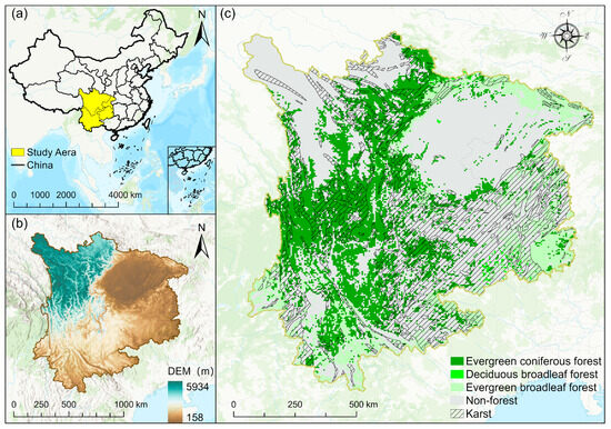
Figure 1.
(a) Geographic location of study area; (b) elevation distribution; (c) karst regions and forest type distribution; the various colors indicate the different types of forests.
2.2. Data and Pre-Processing
2.2.1. MODIS Reflectance Dataset
The MCD43C4 product was used to calculate NIRv, providing nadir BRDF-adjusted reflectance (NBAR) data, corrected by the BRDF (Bidirectional Reflectance Distribution Function). NBAR normalizes reflectance by accounting for BRDF effects using data over a 16-day period. The MCD43C4 product provides daily Level 3 gridded data for reflectance data visibility, using a sinusoidal projection with a 0.05° spatial resolution [38]. Pixels with low BRDF inversion quality (more than 50% fill values) were excluded based on quality indices [25]. NIRv for the study area was then derived through band calculations, and missing data were filled using the mean seasonal cycle, which was calculated by averaging the same calendar month across all available years [39]. NIRv is a vegetation index, calculated by multiplying the normalized difference vegetation index (NDVI) with near-infrared reflectance. It reflects vegetation photosynthesis to a certain extent, effectively isolating vegetation signals while reducing soil noise in the spectral data [40].
2.2.2. Solar-Induced Chlorophyll Fluorescence (SIF) Dataset
SIF data originated from the GOSIF global fluorescence dataset, which integrates OCO-2 SIF measurements with MODIS and meteorological reanalysis inputs. GOSIF provides a high spatiotemporal resolution global SIF dataset, offering 8-day or monthly SIF retrievals between 2000 and 2023 at 0.05° spatial resolution [41].
2.2.3. Forest Cover Dataset
This study used the European Space Agency (ESA) Climate Change Initiative (CCI) annual land cover dataset at a 300 m resolution. The CCI dataset, based on the Land Cover Classification System (LCCS) developed by the United Nations Food and Agriculture Organization (UN FAO), divides the Earth’s surface into 22 classes, among which five represent forest types: evergreen needleleaf forest, deciduous needleleaf forest, evergreen broadleaf forest, deciduous broadleaf forest, and mixed forest. Using the forest distribution information provided by the dataset, we first delineated forest pixels in Southwest China and resampled the original data to 0.005° (approximately 500 m). Then, through spatial aggregation, we obtained the dominant forest type (mode) within each 0.05° pixel and calculated the proportion of forest pixels to determine the forest cover percentage for each 0.05° pixel. To align with the AR(1) variable, we averaged the forest cover percentages from 2001 to 2020 as input for the model.
2.2.4. Forest Loss Dataset
Forest loss data were sourced from the Hansen Global Forest Change V1.10 dataset [42], which provides global forest cover, loss, and gain data at a 30 m resolution since 2000. This dataset utilizes high-resolution satellite imagery and machine learning algorithms for fine classification and change detection. In this study, we considered any pixel that experienced forest loss during the period 2001–2020 as a forest loss pixel. The forest loss fraction at 0.05° resolution was obtained by resampling the 30 m resolution data and calculating the proportion of such loss pixels within each grid cell.
2.2.5. Canopy Height Dataset
For canopy structure, this study utilized the ratio γ (RH25/RH100), where RH25 and RH100 denote the 25% and 100% energy return heights (i.e., the canopy top height), both derived from the ATL08 data product of ICESat-2. The canopy height metrics RH25 and RH100 in the ATL08 product were estimated based on measurements from the Advanced Topographic Laser Altimeter System (ATLAS) on the ICESat-2 satellite. We acquired all ICESat-2 ATL08 products from 2018 to 2022, extracted the RH100 and RH25 metrics, obtained the spatial distribution of RH100 and γ data, and finally processed the data to generate complete RH100 and γ datasets of forest in Southwest China at a 0.05° resolution. In fully developed forests, a high γ value may indicate dense understory vegetation that restricts the penetration of lidar photons [43].
2.2.6. Forest Age Dataset
Forest age data were sourced from a global forest age dataset with a 1 km resolution, which provides estimates of forest age distribution around 2010. This dataset was generated using machine learning methods trained on over 40,000 forest inventory plots along with biomass and climate data. The assessment showed that the dataset has relatively strong predictive power, distinguishing between old-growth and non-old-growth forests while estimating their respective ages [44]. To match the spatial resolution of AR(1), the data were resampled to 0.05° through spatial aggregation.
2.2.7. Standardized Precipitation Evapotranspiration Index (SPEI) Dataset
Drought patterns were determined using the SPEI dataset, considering time scales between 1 and 48 months [45]. SPEI across different time scales reflects varying drought patterns; typically, a longer time interval reduces discrepancies observed in monthly data while emphasizing features at seasonal and annual levels. SPEI integrates both precipitation and evaporation, two key determinants of drought, and is well-suited for characterizing droughts at seasonal, semi-annual, and annual scales in the Southwest China. In this study, data at a 3-month scale were selected, with a spatial resolution of 0.5°. To minimize potential errors arising from incompatible spatial resolutions with different datasets, the dataset was resampled to 0.05° through bilinear interpolation.
SPEI serves as a measure of moisture conditions, where monthly water deficits indicate either surplus or shortage of moisture. The methodology for calculating SPEI involves several steps: initially, the potential evapotranspiration (PET) is assessed on a monthly basis, followed by determining the difference between monthly precipitation and evapotranspiration. Subsequently, a cumulative series of water deficits is formulated across various timescales, and the probability distribution is analyzed. Ultimately, this cumulative series is standardized for each month to yield the corresponding SPEI value [46]. These SPEI values are classified into five distinct levels that denote varying degrees of drought severity (Table 1).

Table 1.
SPEI drought classification table.
2.2.8. Meteorological Dataset
This study utilized meteorological data including photosynthetically active radiation (PAR), precipitation, and vapor pressure deficit (VPD). The PAR data were derived from the Global Land Surface Satellite (GLASS) PAR product, which is calculated based on MODIS spectral data, cloud products, and the GLASS albedo product. The dataset offers global PAR information spanning 2000 to 2020 with a spatial resolution of 0.05°. VPD (hPa) was calculated based on temperature (T) and dew point temperature (Td) [47], with the T and Td data obtained from the monthly summaries of ERA5 Land hourly data with a 0.1° resolution. Precipitation data were obtained from the Global Precipitation Measurement (GPM) precipitation dataset with a 0.1° resolution and were used to generate monthly precipitation distributions for the Southwest region. Precipitation, as well as the T and Td used for calculating VPD, were all provided by the Google Earth Engine (GEE) platform. To ensure consistency in spatial resolution, these datasets were resampled to 0.05°. The PAR and precipitation data have daily and hourly temporal resolutions, respectively. They were first temporally aggregated by calculating monthly means for PAR and monthly sums for precipitation, followed by spatial resampling.
2.2.9. Land Surface Temperature (LST) Dataset
The LST data for this study were sourced from the MODIS MOD11A1 product, offering a 1-day temporal resolution and 1 km spatial resolution. MOD11A1 has undergone radiometric, atmospheric, and geometric corrections. After applying quality control to the MOD11A1 data, resampling was performed to obtain LST data for the forested areas of Southwest China at a 0.05° resolution for the period from 2001 to 2020 [48]. Similarly, to maintain temporal consistency with the AR(1) timescale, the LST data were temporally aggregated to obtain monthly-scale data.
2.2.10. Soil Moisture Dataset
Soil moisture (SM) data were obtained from the TerraClimate dataset, a global monthly high-resolution (1/24°, ~4 km) climate dataset that includes variables such as temperature, precipitation, wind speed, and derived hydrological metrics. The soil moisture values are generated using a modified Thornthwaite–Mather one-layer water balance model, which integrates precipitation, reference evapotranspiration (calculated using the Penman–Monteith method), remotely sensed plant-extractable water capacity, and snow water equivalent to simulate end-of-month soil water storage. A lower threshold of 10 mm was applied to ensure ecological relevance [49]. The TerraClimate SM data from 2001 to 2020 were obtained via the GEE platform. To match the spatial resolution of AR(1), the data were resampled to 0.05° using nearest-neighbor interpolation.
2.2.11. Topographic Dataset
Considering the target spatial resolution, topographic data were derived from the 90 m resolution SRTM Digital Elevation Model (DEM). Slope, aspect, and the Topographic Wetness Index (TWI) were calculated based on the DEM using ArcGIS10 .7. These topographic variables were then resampled and spatially aggregated by averaging to obtain their distribution at a 0.05° resolution.
2.3. Methods
2.3.1. Calculation of the Resilience Indicator AR(1)
Experimental designs under the framework of low-dimensional dynamical systems have demonstrated that as a system approaches a critical threshold, lag-1 autocorrelation increase. Once this threshold is surpassed, a bifurcation-induced transition occurs, referred to as Critical Slowing Down (CSD) [11,50]: As the system’s current equilibrium state becomes less stable, its response to short-term perturbations becomes more sluggish. This loss of resilience is generally characterized by the rate at which a system returns to its initial state after a disturbance, reflecting a weakening of the negative feedback maintaining the stability of forest ecosystems [51]. It may also manifest as an increase in variance over time. However, unlike AR(1), variance is more susceptible to other mechanisms, which may cause it to either increase or decrease as the system approaches a critical threshold [52]. In this study, we used a first-order autoregressive model to calculate the AR(1) of the time series within each pixel. Scheffer et al. clarified the direct correspondence between AR(1) and the principle of CSD through the derivation of system dynamics equations [11]. Smith et al. further validated the theoretical link between AR(1) and empirical recovery rates using global satellite data, suggesting that AR(1) can serve as an early warning indicator of declining ecosystem resilience [22]. In many fields, including climate and ecology, increases in AR(1) have been used to detect CSD and provide early warning signals before a bifurcation-induced state shift occurs [24,32]. Generally, a high AR(1) value indicates low resilience and is strongly correlated with forest mortality rates [53].
is the time series of the NIRv, and is the time series at moment t + 1, which corresponds to the NIRv time series lagged by one month. is the autoregressive coefficient, and the error term.
Before estimating AR(1), the NIRv time series was decomposed into seasonal, trend, and residual components using the Seasonal and Trend decomposition using the Loess (STL) method. The decomposition involves an iterative smoothing process of the trend and seasonal components, which are subsequently removed from the original series to derive the residuals. This process was executed using the STL function from the “stats” package (v4.2.1) in R (v4.3.2) [54]. In this function, we evaluated AR(1) time series by adjusting trend window lengths and using different datasets to assess the robustness of the detrending method (Figure A1).
The ar.ols() function from R’s “stats” package (v4.2.1) was applied to the NIRv time series’ residual component to estimate AR(1), using a four-year (48 months) sliding window to construct the AR(1) time series for each pixel. The determination of trend and statistical significance of both the AR(1) and the mean NIRv time series was determined using Kendall τ and p-values. Kendall τ evaluates the correlation between two random variables based on the ranks of data objects. The target objects for analysis should be ordered categorical variables. Before conducting Kendall’s correlation analysis, it is essential to check that the data meet two assumptions: the variable data should be ordinal or continuous, and there should be a monotonic relationship should exist between them. In this study, one of the variables is time. Kendall τ values were calculated using the cor.test() function from R’s “stats” package (v4.2.1), with a 0.95 confidence level to evaluate trends in AR(1) and NIRv. A positive Kendall τ (p < 0.05) signifies a significant increase in AR(1) and mean NIRv, whereas a negative τ (p < 0.05) indicates a significant decrease in these values.
2.3.2. Definition of ALR
We obtained long-term AR(1) using NIRv and SIF data, which are closely related to photosynthesis. By combining SPEI and prolonged periods of exceptionally high AR(1) values, we identified abnormally low resilience (ALR) caused by drought (ALR_NIRv, ALR_SIF) (Figure A2). ALR is determined when AR(1) exceeds the threshold (the 80th percentile) and persists for at least three months. Abnormally low NIRv and SIF(AL_NIRv, AL_SIF) are defined as values below the threshold (the 20th percentile) that last for at least three months.
2.3.3. XGBoost Model and Shapley Explanation Framework
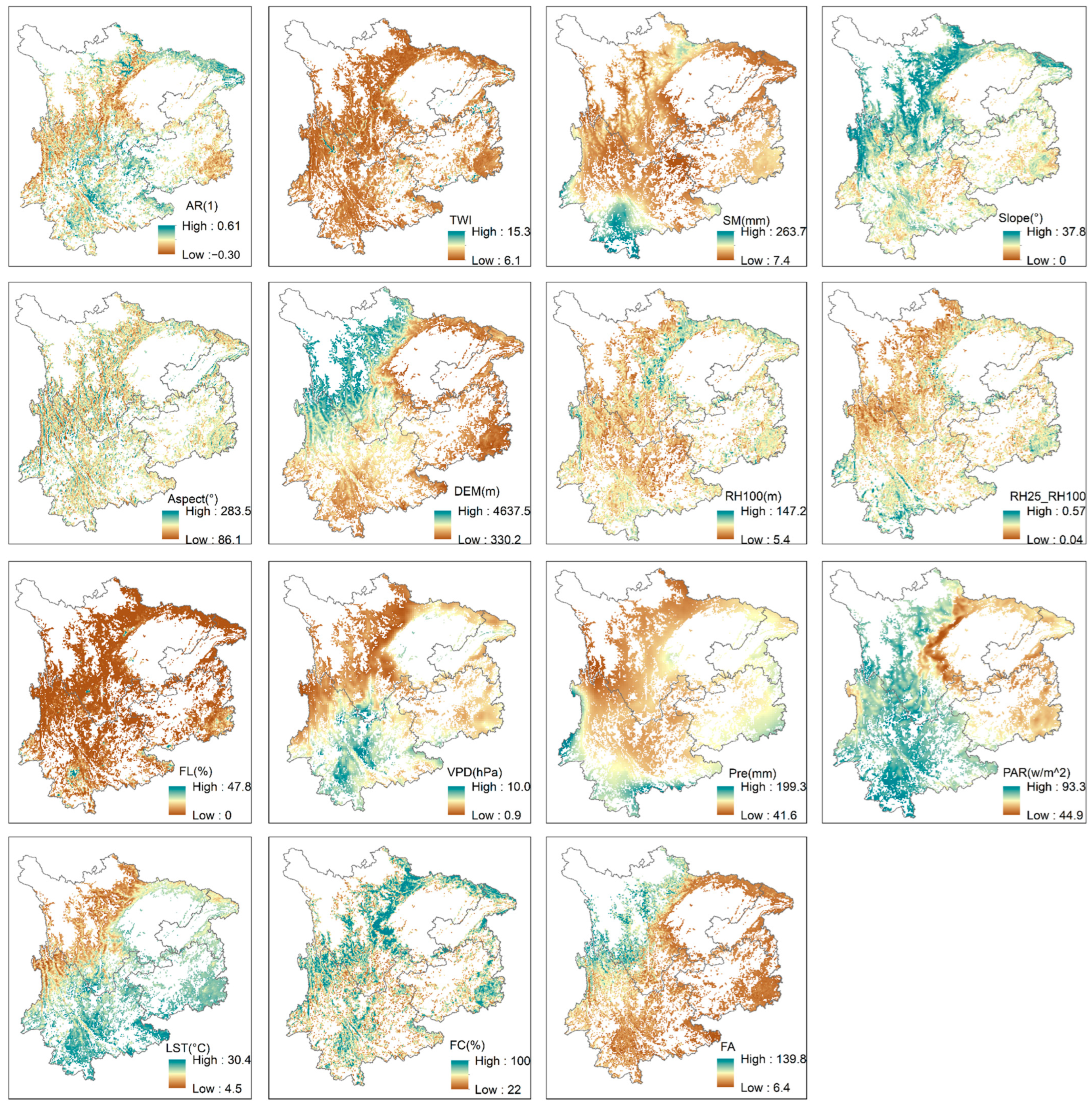
Extreme Gradient Boosting (XGB) enhances the Gradient Boosting Decision Tree (GBDT) algorithm through the Boosting ensemble approach. XGB applies regularization methods, including shrinkage, to manage model complexity and prevent overfitting by adjusting the weights of newly added trees at each enhancement step [55]. Previous studies have shown that XGBoost can deliver more stable results and more efficient training when dealing with large and structurally complex datasets, while effectively preventing overfitting [56]. As a boosting method, XGBoost offers strong interpretability of variables; when combined with SHAP analysis, it enables clear, individual-level explanations of variable influence. This is particularly suitable for exploring interactions and nonlinear relationships among variables. The use of XGBoost and SHAP to investigate nonlinear relationships between driving factors and response variables has become well established and has been widely applied across various fields [57,58,59]. In this study, we classified forests in Southwest China into coniferous and broadleaved types and developed two separate nonlinear XGBoost models. Using 14 variables—including climate factors, tree age, topography, forest cover, and forest loss (Table A1)—we simulated multi-year mean monthly AR(1) values. The full names of the variables and their corresponding abbreviations are listed in Table 2. Regarding the treatment of missing values during modeling, any pixel with a missing value in any input variable was excluded from the modeling process.
Table 2.
Driving factors and their abbreviations used in the XGBoost model.
We employed the SHAP framework to assess the impact of drivers on forest resilience in Southwest China [60]. This approach quantifies the individual contribution of each factor to the predicted outcome. Specifically, the SHAP value for each feature reflects its marginal effect on the prediction, isolating its influence while holding all other factors constant. The SHAP value is calculated as the sum of differences between the baseline value (the mean of all predicted values) and the current prediction, similar to the method used in partial dependence regressions. Rather than modeling AR(1) directly, this method focuses on the difference between predicted and expected AR(1) values. Higher SHAP values indicate a greater contribution of a particular feature to AR(1). In this study, SHAP values were used to examine the marginal effects of potential driving factors to AR(1), with positive SHAP values indicating an increase in AR(1) driven by a specific variable. SHAP is a model interpretability method based on cooperative game theory [61], which approximates the original black-box model f(x) by constructing an interpretable surrogate model g(z′). Its mathematical formulation can be expressed as
where represents the number of features; is the mean prediction for all samples; indicates whether the j-th feature is included (1) or excluded (0) from the coalition; is the SHAP value for feature.
To derive the SHAP values , the method considers all possible feature subsets that exclude the target feature j. The marginal contribution of adding feature j to subset S is given by the difference in model outputs . Here, is the expected model output conditional on the features in subset S. The SHAP value is then calculated as the weighted average over all such subsets:
This formulation satisfies three key properties: local accuracy (the sum of SHAP values equals the model output), missingness (missing features receive zero attribution), and consistency (increased model dependence on a feature leads to a non-decreasing SHAP value) [62].
A visual inspection of the SHAP value plots reveals that there may be inflection points where the relationship between a driving factor and its associated SHAP value (i.e., the slope or intercept) changed abruptly. To quantitatively validate this, we used the R package “chngpt” (v2023.06.14) to identify the points where the relationship between SHAP values and driving factors shifts [63].
3. Results
3.1. Spatio-Temporal Patterns of Forest Greening and Resilience in Southwest China
We found that the greening of forests and the decline in resilience across Southwest China occurred simultaneously since 2008. From 2001 to 2008, the NIRv time series exhibited a significant upward trend (τ = 0.97), with 85.97% of the region showing increased NIRv (Figure 2d). This trend became more pronounced from 2009 to 2020, with the proportion of pixels exhibiting increased NIRv rising to 92.95% (Figure 2e), suggesting that forests in Southwest China have undergone sustained greening over the past two decades. However, the AR(1) time series identified a critical breakpoint in September 2008. During 2001–2008, AR(1) displayed a significant negative trend (τ = −0.84, p < 0.001), indicative of increasing resilience, which shifted to a positive trend from 2009 to 2020 (τ = 0.66, p < 0.001), reflecting a transition to declining resilience (Figure 2a). Notably, 69.01% of forest pixels experienced enhanced resilience between 2001 and 2008 (Figure 2d). In contrast, only 32.60% of pixels exhibited increased resilience during the period from 2009 to 2020 (Figure 2e).
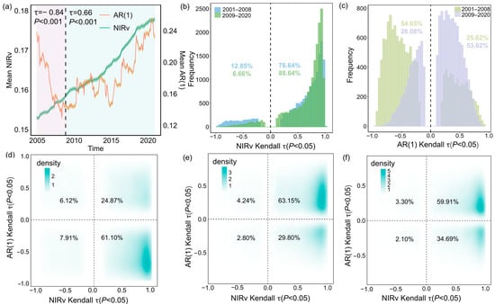
Figure 2.
Long-term changes in forest dynamics and resilience in Southwest China from 2001 to 2008, 2009 to 2020, and 2001 to 2020. The solid lines in (a) represent the regionally mean NIRv (green) and AR(1) (red), with shaded areas denoting the respective 95% confidence intervals. Mean values of NIRv and AR(1) are plotted at the conclusion of each sliding window. The black dashed line marks the breakpoint in the time series. (b,c) Histograms of Kendall τ values for the NIRv and AR(1) time series, contrasting the periods 2001–2008 and 2009–2020. (d–f) Cumulative density distributions of Kendall τ relationships between NIRv and AR(1) shown for 2001–2008 (d), 2009–2020 (e), and 2001–2020 (f). Numeric labels within the four quadrants indicate the percentage of pixels in each quadrant. For visual clarity, raster data with non-significant Kendall τ values (p > 0.05) are excluded from the figure. N = 17,754.
Our findings remained consistent when using different sliding window length and trend window for AR(1) calculations (Figure A3 and Figure A4). Notably, when resilience was measured by variance instead of AR(1), a similar pattern was observed, with resilience first increasing and then declining (Figure A5). These consistent patterns offer robust evidence of notable changes in forest resilience, which have profound implications for the persistence of forest ecosystems in Southwest China.
The spatial patterns of forest dynamics and resilience changes also exhibited regional differences. From 2001 to 2008, Sichuan and most areas of Guizhou showed a trend of simultaneous enhancement in forest greenness and resilience. However, in central Yunnan, despite the increase in forest greenness, resilience declined. A few areas in northern Yunnan experienced both forest browning and loss of resilience (Figure 3a). During the period from 2009 to 2020, although forest greenness continued to increase in most areas of the Sichuan Basin and Guizhou, resilience in these regions showed a declining trend (Figure 3b). Overall, over the two decades, except for a small portion of northern Yunnan and western Sichuan that experienced browning, more than half of the forests exhibited greening with a decline in resilience (59.91%). In contrast, only around one-third of forests showed signs of both greening and increased resilience (34.69%) (Figure 3c). This pattern highlights the complex relationship between greenness and resilience in the forest ecosystems of Southwest China.

Figure 3.
Spatial patterns of forest dynamics and resilience changes over the two decades. (a) 2001–2008, (b) 2009–2020, and (c) 2001–2020. Similarly, for visual clarity, raster pixels with non-significant Kendall τ values (p > 0.05) are excluded from the figure. ↑ indicate an increase, ↓ indicate a decrease.
3.2. Determination of the Dominant Factors Affecting Forest Resilience
3.2.1. Factors Affecting Forest Resilience
We used machine learning models to identify the key drivers of changes in forest resilience for coniferous and broadleaf forests in Southwest China and to evaluate their relative contributions. The coniferous forest dataset contained 11,523 samples, while the broadleaf forest dataset included 6231 samples. Both datasets were split into training and testing sets at a ratio of 75% to 25%. Hyperparameter tuning was performed using Bayesian optimization combined with five-fold cross-validation. Ultimately, the models achieved R2 values of 0.66 and 0.61 for predicting AR(1) on the test sets of coniferous and broadleaf forests, respectively (Figure A6). Based on permutation-based variable importance rankings (Figure 4), the key drivers significantly affecting AR(1) differed between the two forest types. For coniferous forests, the top five drivers were elevation, LST, PAR, Pre, and VPD, while for broadleaf forests, the top five were PAR, SM, Pre, elevation, and LST. Notably, climate factors dominated the main drivers of AR(1) in both forest types, highlighting the critical influence of climate on forest resilience in Southwest China.
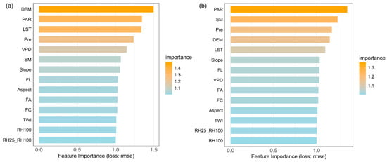
Figure 4.
Importance ranking of potential drivers affecting resilience in coniferous and broadleaf forests. Variable importance was calculated using a permutation-based method, which measures the change in model prediction error after randomly shuffling each variable’s values. A ratio of 1 indicates no significant change in prediction error before and after permutation; the larger the ratio, the greater the variable’s impact on model predictions, and thus the higher its importance. (a) Coniferous forests. (b) Broadleaf forests.
To evaluate the relationship between changes in forest resilience and various driving factors, this study used SHAP values to quantify the impact of each driver on model outputs (Figure 5, Figure 6 and Figure 7). The results showed that LST had different effects on the resilience of coniferous and broad-leaved forests. In coniferous forests, forest resilience gradually decreased with increasing LST, a trend reflected by the increasing SHAP values. When LST exceeded 16.8 °C, its negative impact on resilience became more pronounced, and the extent of resilience loss further intensified. In broad-leaved forests, resilience gradually increased with rising LST; however, when LST exceeded 21.3 °C, its effect on resilience turned negative. With increasing elevation, resilience improved progressively in both coniferous and broad-leaved forests. A similar trend was also observed for Pre. PAR exerted a significant negative effect on the resilience of both forest types, but in broad-leaved forests, the impact exhibited a phased pattern: when PAR exceeded 66 w/m2, its negative effect on resilience weakened. Increased SM helped enhance resilience in coniferous forests, while in broad-leaved forests, SM values below 93 mm were beneficial to resilience. However, once this threshold was exceeded, its effect turned negative. VPD had a similar influence on the resilience of both coniferous and broad-leaved forests, with a turning point at a certain threshold. Below this value, the effect was positive, while above it, the effect became negative.
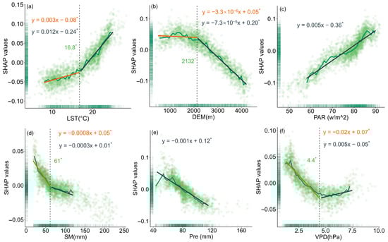
Figure 5.
The impact of key drivers on resilience in coniferous forests based on SHAP values: (a) LST, (b) DEM, (c) PAR, (d) SM, (e) Pre, and (f) VPD. The black dashed line represents the change point detected using the “chngpt” package, and the green number indicates the value of the change point. Asterisks denote statistically significant change points (p < 0.05). The green solid line represents the median SHAP values for 50 bins of the data. The orange and gray solid lines represent the linear regressions before and after the change point, respectively, with corresponding regression equations provided. The slope units correspond to the variables on each x-axis. Asterisks also indicate statistically significant regression slopes (p < 0.05).
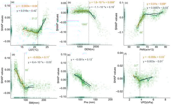
Figure 6.
The impact of key drivers on resilience in broadleaf forests based on SHAP values: (a) LST, (b) DEM, (c) PAR, (d) SM, (e) Pre, and (f) VPD. Asterisks also indicate statistically significant regression slopes (p < 0.05).
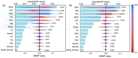
Figure 7.
Relative importance and marginal contributions of driving factors to AR(1) in coniferous and broadleaf forests. The blue bar plots on the left show the mean absolute SHAP values of each variable, which quantify the average magnitude of each factor’s contribution to the model predictions across all samples. Larger values indicate greater overall explanatory power for AR(1), with specific values labeled in black. The scatter plots on the right display the normalized SHAP values for each sample, representing the marginal contributions of each factor—i.e., the direction and magnitude of their influence on AR(1) at the individual level. Point colors indicate the original value of the corresponding variable. (a) Coniferous forests; (b) Broadleaf forests.
3.2.2. Spatial Distribution of the Main Factors for Forest Resilience
DEM had the most significant influence on coniferous forest areas, accounting for 32.9%, and was mainly distributed in western Sichuan (Figure 8a). This was followed by LST and PAR, with contribution rates of 26.8% and 20.0%, respectively, mainly affecting most areas of Yunnan Province and central Sichuan. The impacts of Pre and VPD accounted for 9.0% and 6.0%, respectively. The regions dominated by Pre were mainly located in northern Yunnan and northern Sichuan, while those dominated by VPD were primarily in central Yunnan and parts of northern Sichuan. In broadleaf forests, PAR was the most dominant driving factor, accounting for 29.9%, and was mainly distributed in eastern Guizhou and central Sichuan. This was followed by SM and Pre, with contribution rates of 27.7% and 20.9%, mainly concentrated in northeastern Sichuan and eastern Guizhou. DEM and LST had relatively smaller impacts in broadleaf forests, accounting for 9.7% and 9.2%, respectively.

Figure 8.
Spatial distribution of key drivers influencing forest resilience in Southwest China. (a) Spatial distribution of the dominant driving factor influencing forest resilience: for each pixel, the driving factor with the highest SHAP value is identified as the dominant factor. (b) Spatial distribution of SHAP values of the dominant driving factor: representing the SHAP value of the most influential factor in each pixel. (c) Proportions of the dominant driving factors in coniferous forests, and (d) proportions of the primary driving factors in broadleaf forests.
It is worth noting that in coniferous forests, DEM and PAR had negative contributions to AR(1), while LST and Pre showed positive contributions, indicating higher resilience in the regions associated with the former. In broadleaf forests, PAR and Pre mainly showed negative contributions, while SM had a positive effect on AR(1) in eastern Sichuan and a negative effect in eastern Guizhou. Among the negative factors, PAR had the most significant negative impact, while among the positive factors, LST had the strongest positive effect (Figure 8b).
3.3. Responses of Forest Resilience to Drought Events in Southwest China
3.3.1. Dynamic Changes in ALR Area Fraction
The significant decline in forest resilience, along with the notable reduction in SIF and NIRv indices, indicates a weakening of forest vitality and productivity. The area fraction of ALR calculated from SIF and NIRv satellite indices exhibited a consistent trend over the time series. During the extreme drought event of 2009–2010, Southwest China saw an exacerbation of drought conditions, resulting in increases in area fractions of ALR_SIF, ALR_NIRv, AL_SIF, and AL_NIRv. Notably, the increases in the area fractions of AL_SIF and AL_NIRv were more pronounced compared to those of ALR_NIRv and ALR_SIF (Figure 9a,c). For the prolonged drought from 2011 to 2013, all four indices reflected the impacts of drought, showing an upward trend. In contrast, during the drought event in 2006, while area fractions of AL_NIRv and ALR_SIF increased, the magnitude of this increase was relatively limited, and the changes in ALR_SIF and ALR_NIRv were not significant, even showing a declining trend during the drought.
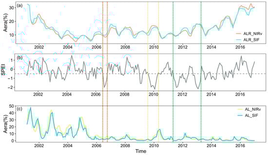
Figure 9.
Time series of drought severity and ALR_NIRv, ALR_SIF, AL_NIRv, and AL_SIF areas. (a) Proportions of ALR_NIRv and ALR_SIF areas. (b) Long-term variation of SPEI-03, with the gray dashed line indicating SPEI = −0.5, and drought severity classified according to Table 1. The colored dashed lines represent drought events in the Southwest China forest from 2001 to 2020, specifically in 2006, 2009/2010, and 2011–2013. (c) Proportions of AL_NIRv and AL_SIF areas.
Compared to the severe drought event of 2009/2010, forests exhibited a milder response to the drought in 2006, as evidenced by the changes in the area fractions of ALR_NIRv, ALR_SIF, AL_NIRv, and AL_SIF. Between 2009 and spring 2010, Yunnan and Guizhou experienced nearly eight consecutive months of severe drought, whereas the 2006 drought was shorter in duration and less intense. Moreover, the similar temporal trends observed in ALR_SIF, ALR_NIRv, AL_SIF, and AL_NIRv during the drought highlight their potential for detecting the gradual temporal dynamics of forest recovery under drought conditions.
3.3.2. Spatial Patterns of ALR
We focused on the extreme drought event of 2009/2010 in the study to assess the spatial response of ALR_NIRv, ALR_SIF, AL_NIRv, and AL_SIF to drought. The drought event began in September 2009, originating in eastern and northwestern Yunnan, southwestern Guizhou, and eastern Chongqing. It gradually expanded, eventually reaching eastern and northwestern Sichuan by February 2010. Southwestern Guizhou, eastern Yunnan, and most of Chongqing experienced the longest drought (over 10 months) and the most severe conditions (Mean SPEI−03 < −1.5). In contrast, Sichuan and western Yunnan faced shorter, less intense droughts (Figure 10a,d). By 2010, extensive areas of ALR_NIRv, ALR_SIF, AL_NIRv, and AL_SIF were observed in western and southern Sichuan, much of Yunnan, eastern Guizhou, and scattered areas of Chongqing. These indices appeared across most drought-affected regions, with relatively consistent spatial distribution patterns. Notably, despite the milder and shorter drought in western Sichuan and Yunnan, signals of AL_NIRv and AL_SIF were still detected.
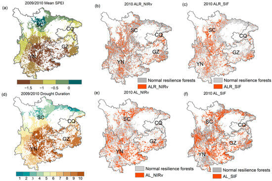
Figure 10.
(a) Spatial distribution pattern of the 2009/2010 extreme drought event, (b) ALR_NIRv in Southwest China forests in 2010, (c) ALR_SIF, (d) spatial distribution pattern of the drought duration for the 2009/2010 extreme drought event, (e) AL_NIRv, (f) AL_SIF. Abbreviations: CQ (Chongqing), SC (Sichuan), GZ (Guizhou), YN (Yunnan).
4. Discussion
In this study, we observed that around September 2008, the AR(1) time series of Southwest forests shifted from a gradual decline to a steady increase, indicating a reduction in resilience, while the NIRv time series showed continuous growth. Our result indicated the decoupling of forest greening and resilience trends post-2008 across Southwest China. From 2001 to 2008, more than half (61.10%) of the forests experienced both increased greenness and enhanced resilience. This simultaneous enhancement likely reflects the widespread implementation of ecological engineering projects in the early 2000s, which reduced human disturbances, increased forest cover, and benefited from favorable environmental conditions. However, between 2009 and 2020, forest greening shifted from widespread resilience gain to resilience loss. Our findings suggest that extreme drought events may have contributed to this loss of forest resilience during 2009–2020 (Figure 9).
Our study found that the primary drivers of resilience changes differ between coniferous and broadleaf forests in Southwest China. For coniferous forests, the main drivers of resilience included elevation, PAR, LST, precipitation, and VPD. In broadleaf forests, the primary drivers were PAR, SM, precipitation, elevation, and LST. In Southwest China, elevation was the dominant driver of resilience in coniferous forests, which may be attributed to the distinct altitudinal distribution between coniferous and broadleaf forests. Coniferous forests are predominantly found at high elevations, whereas broadleaf forests are mostly distributed in low to mid-elevation areas. High-elevation regions are characterized by harsher climatic conditions, and coniferous forests have developed adaptive traits over long-term evolution to cope with extreme environments such as low temperatures and strong winds [64]. Regardless of forest type, resilience generally increases with elevation. This may be because, under the background of global warming, the rate of temperature increase at high elevations is significantly higher than at lower elevations, and winter temperatures are rising faster than those in spring. Such conditions may alleviate low-temperature limitations for trees in high-elevation regions, enhance photosynthetic rates, and lead to an earlier onset of the growing season, thereby giving them a competitive advantage [65,66]. In contrast, trees in low-elevation areas face increasing competition for soil moisture, a challenge that becomes particularly pronounced when responding to environmental disturbances [33].
Coniferous and broadleaf forests exhibit distinct responses in resilience to changes in LST. In coniferous forests, resilience gradually decreases with increasing LST, likely due to their lower stomatal conductance and weaker transpiration capacity, making them more susceptible to water stress. Elevated LST intensifies evapotranspiration, thereby inhibiting the recovery of coniferous forests [67]. Moreover, after forest fires, higher surface temperatures can suppress the germination and growth of conifer seedlings, as increased heat exacerbates soil drying. In contrast, broadleaf species may gain a competitive advantage in such conditions due to their higher water-use efficiency [68]. However, when LST exceeds a certain threshold in broadleaf forests, it also begins to suppress their resilience. Continued increases in LST reduce soil moisture availability, limiting the trees’ ability to absorb water through their roots, which in turn slows growth and diminishes the overall resilience of the ecosystem.
This study found that PAR has a negative impact on forest resilience in both coniferous and broadleaf forests. While previous research has identified a positive relationship between an ecosystem’s maximum photosynthetic capacity and average light intensity [69], higher PAR not only enhances the potential for photosynthesis but also extends daylight hours and intensifies transpiration. Forest ecosystems are less adaptable to high PAR, and excessive transpiration can lead to rapid internal water loss in trees, especially when soil moisture is insufficient. This complex interaction suggests that while higher solar radiation promotes carbon uptake, it can also exacerbate water stress in forests [70].
The increases in LST and PAR are often accompanied by an increase in VPD, leading to drier atmospheric conditions. Our findings revealed that forest resilience tended to increase with VPD within a normal range, but when VPD exceeded a threshold, resilience experienced a sharp decline. The primary impact of elevated VPD on forest–atmosphere gas exchange is through its influence on tree physiological processes, particularly stomatal regulation. As VPD increases, trees reduce stomatal opening to conserve water, which inadvertently limits CO2 absorption, leading to reduced photosynthesis and even result in tree mortality [71,72,73]. Additionally, extreme VPD can indirectly affect trees through the high temperatures that accompany it, increasing respiration and further reducing net CO2 uptake during periods of abnormal VPD [74]. In addition to the direct physiological effects of VPD on trees, soil moisture—an essential component of water supply in forest ecosystems—also plays a crucial role in regulating forest resilience. Yao et al. reported that vegetation recovery time after drought shortens with increasing soil moisture [75]. Moist soils with high organic matter accumulation can continuously supply nutrients to forests, thereby enhancing their resilience [76]. However, in the broadleaf forests of Southwest China, excessive soil moisture can suppress resilience, possibly due to the inhibition of root respiration under overly wet conditions, which in turn weakens forest recovery capacity.
The dominant driver of forest resilience in central and eastern Yunnan is LST. The consistent average LST of approximately 30 °C over this specified region has been empirically linked to an escalation in wildfire occurrences [77,78]. The prevalent evergreen coniferous forest cover, characterized by an intricate and multifarious understory abundant in combustible materials [79], further exacerbates the vulnerability to wildfires. Wildfires not only lead to increased tree mortality but also affect post-fire recovery and species composition due to the resulting surface warming [69]. In the center of Sichuan and Guizhou, the primary driver of forest resilience is PAR. These regions fall within China’s heavy rainfall zone, with annual precipitation averaging between 1000 and 1200 mm. However, dense low-layer monsoon cloud cover reduces irradiance, resulting in an average PAR below 60 w/m2 (Figure A7). Within this range, an increase in PAR positively influences forest resilience [80]. In northeastern Sichuan, eastern Guizhou, and western and southern Yunnan, the dominant drivers of forest resilience are precipitation and soil moisture. Former studies have proven that soil moisture has been gradually decreasing across these regions [81]. Bai et al. [82] assessed the impact of vegetation greening in China, finding that increased evapotranspiration due to greening led to a reduction in water yield. If soil moisture is not replenished by rainfall, the health and survival of forest ecosystems would be severely threatened. Moreover, the dominant forest type in these regions is broadleaf forests. Through field sampling and laboratory tests, Zhou et al. [83] found that the maximum water-holding capacity of broadleaf forests is lower than that of coniferous forests in three forest types within karst regions.
In this study, it is important to note that the research area is located in Southwest China, which is characterized by complex terrain and significant elevation differences, encompassing diverse landforms such as mountains, plateaus, basins, and hills. Such topographic complexity typically exerts substantial influence on the structure and functioning of forest ecosystems. However, the results of this study indicate that topographic factors were not among the primary drivers of forest resilience. This outcome may be attributed to the influence of the research scale. The study employed a spatial resolution of 0.05°, which, while beneficial for improving computational efficiency and model stability at the regional scale, may have obscured local topographic variation and its ecological effects, thereby underestimating the role of topography in the model. In addition, due to the limitations of spatial scale, this study was unable to incorporate more detailed classifications of forest types, which may have masked potential differences in drought responses among functionally distinct forest types. Therefore, future research should incorporate higher-resolution remote sensing data and field-based plot observations to more comprehensively assess the influence of various environmental factors on forest resilience.
Previous studies on vegetation resilience have often quantified post-disturbance recovery based on field data from tree ring widths, or analyzed recovery time and ecosystem damage using remote sensing technology [33,84,85,86]. However, this method is only applicable to natural vegetation systems experiencing major external disturbances, and due to data availability and the seasonal fluctuations in ecosystem responses, it is difficult to apply at large scales. The AR(1) based on the “CSD” theory in this study shows good spatial consistency with the resilience indicator observed in rare external disturbances [22]. It is crucial, however, to recognize that the “CSD” indicator functions more as an early warning signal rather than a definitive marker of critical transitions. In random environments, system shifts often occur before reaching the true bifurcation point [87]. Therefore, a loss of resilience (reflected by an increase in AR(1)) does not necessarily indicate that critical transitions will occur in these regions, highlighting the need for further research on predictive relationship between these metrics we used and the signaling of system state transitions [7].
5. Conclusions
This study examined the spatiotemporal dynamics of forest resilience and greenness in Southwest China. We found a decoupling of forest greening and resilience trends over the past two decades. Since September 2008, forest resilience experienced gradual declines, while forest greenness had an increasing trend. Our results also indicated that since the severe drought events of 2009/2010, large areas of the region’s forests experienced abnormally low resilience. After employing a machine learning algorithm to spatially depict the dominant factors that influencing forest resilience, we found that elevation, PAR, LST, Pre, and SM are the primary factors influencing changes in forest resilience in Southwest China. Among these, elevation plays a key role in shaping the resilience of coniferous forests, while SM and PAR are the main drivers of resilience in broadleaf forests. This discovery not only enhances our understanding of the complexity of forest resilience but also provides a robust scientific foundation for future forest management.
Author Contributions
Conceptualization, T.C. and L.C.; methodology, H.W. and T.C.; validation, H.W. and T.C.; formal analysis, H.W. and T.C.; resources, H.W. and T.C.; data curation, H.W. and T.C.; writing—original draft preparation, H.W.; writing—review and editing, H.W., T.C. and L.C.; visualization, H.W.; supervision, L.C.; funding acquisition, L.C. All authors have read and agreed to the published version of the manuscript.
Funding
This work was supported by the National Natural Science Foundation of China (42201364) and the Opening Funds from Chongqing Jinfo Mountain Karst Ecosystem National Research and Observation Station (JFS2023A02).
Data Availability Statement
Data will be made available on request. The spatial aggregation code has been uploaded to Zenodo: 10.5281/zenodo.15542873.
Acknowledgments
The authors sincerely appreciate the support and assistance from the department of forest management at Nanjing Forestry University, as well as the valuable suggestions provided by fellow graduate students during this study.
Conflicts of Interest
The authors declare no conflicts of interest.
Appendix A
Table A1.
Variables used in the study.
Table A1.
Variables used in the study.
| The Data Type | Products | Time | Native Spatial Resolution | Final Spatial Resolution | Temporal Resolution |
|---|---|---|---|---|---|
| Forest Age | Global 1 km forest age datasets | 2010 | 1 km | 0.05° | year |
| Land cover data | ESA_CCI_Land Cover_300m_Yearly_WorldV2.0.7cds | 2001–2020 | 300 m | 0.05° | year |
| Forest Loss | Hansen Global Forest ChangeV1.10 | 2001–2020 | 30 m | 0.05° | year |
| Canopy Structure | ICESat-2 ATL08 | 2018–2022 | 100 m | 0.05° | 91 d |
| Canopy height | |||||
| SM | TerraClimate | 2001–2020 | 4 km | 0.05° | 1 month |
| T, Td | ERA5-Land Monthly Aggregated | 2001–2020 | 0.1° | 0.05° | 1 month |
| PAR | GLASS PAR | 2001–2020 | 0.05° | 0.05° | 1 d |
| Precipitation | GPM_3IMERGM | 2001–2020 | 0.1° | 0.05° | 1 h |
| LST | MOD11A1 | 2001–2020 | 1 km | 0.05° | 1 d |
| DEM | SRTM | 2010 | 90 m | 0.05° | year |
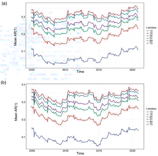
Figure A1.
Tests of robustness for detrending the NIRv and SIF time series. The long-term trend is calculated using different t.window while keeping the seasonal window periodic. (a) The mean AR(1) time series for NIRv under varying t.window settings. (b) The mean AR(1) time series for SIF under varying t.window settings. The results show that despite changes in t.window, the trends for both SIF and NIRv remain relatively stable, confirming that the transition of the AR(1) time series from a negative to a positive trend after September 2008, as described in the main text, is robust to the choice of t.window.
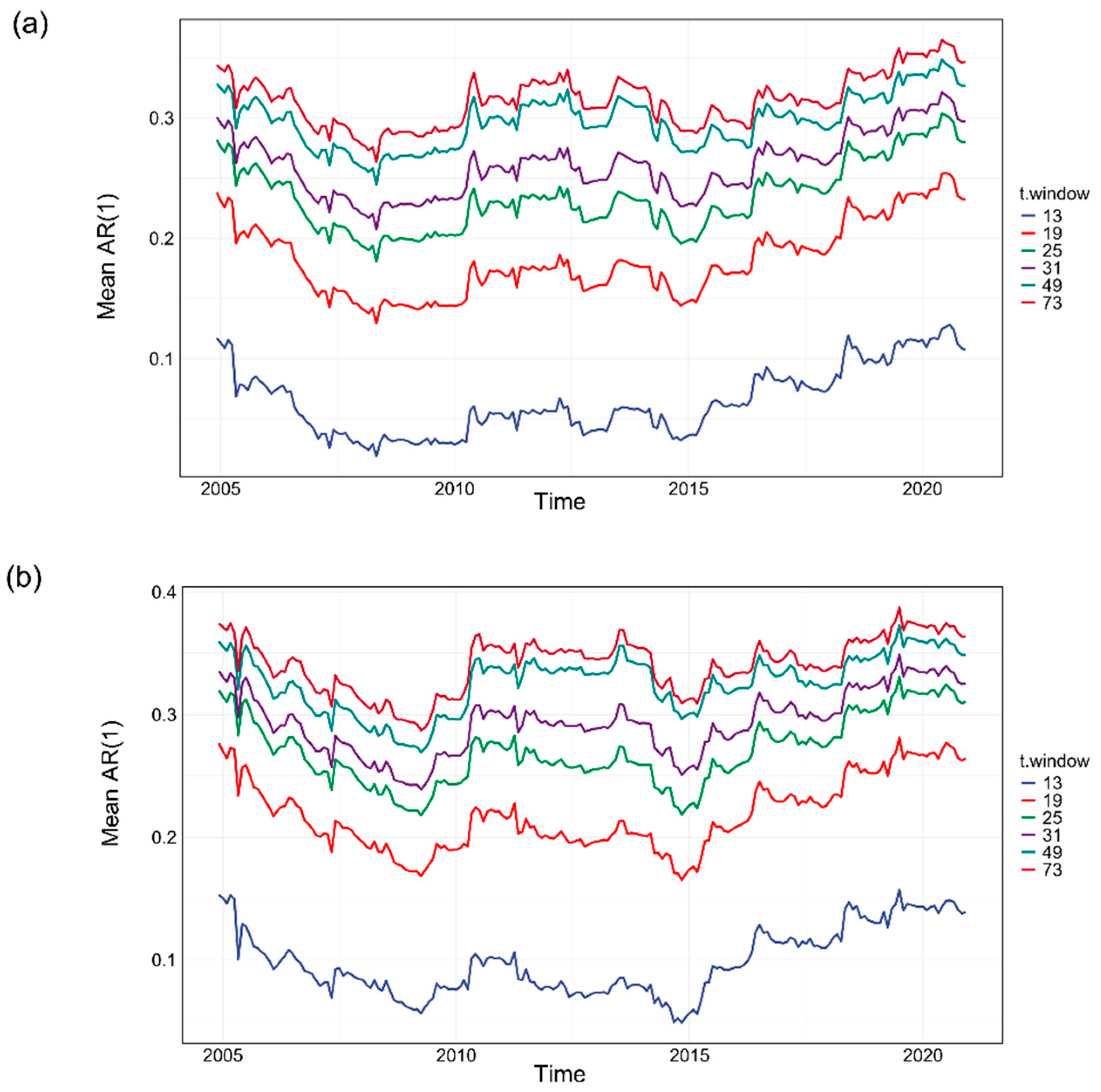
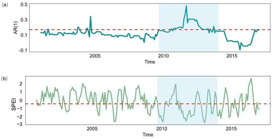
Figure A2.
In a pixel in Southwest China, the time series of forest AR(1) and SPEI is as follows: (a) The long-term time series of AR(1) within the pixel, with the red dashed line representing the 80th percentile value. (b) The long-term time series of SPEI within the pixel, with the red dashed line indicating SPEI = −0.5. The blue background represents the period from 2009 to 2013, during which drought events were frequent in Southwest China.
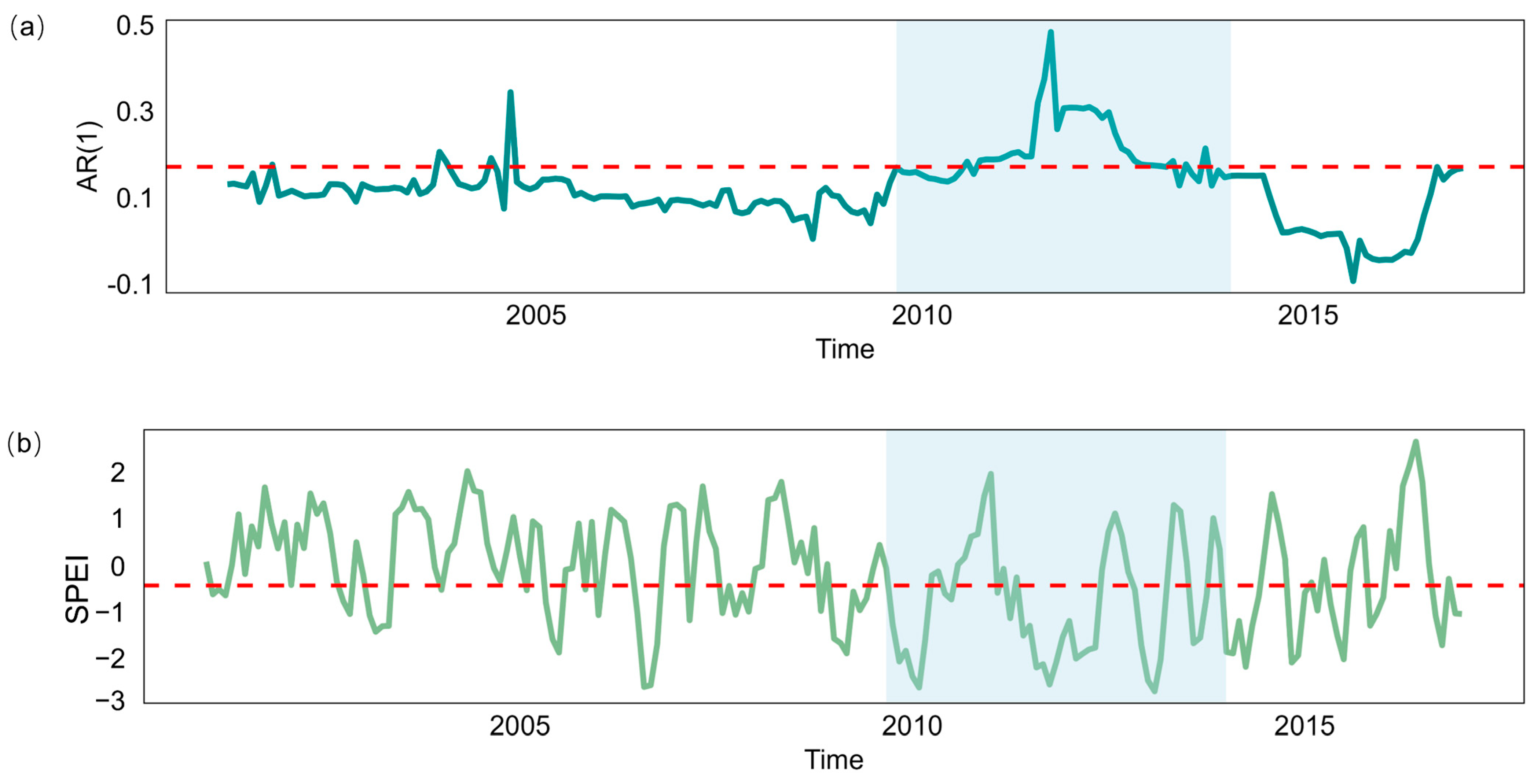
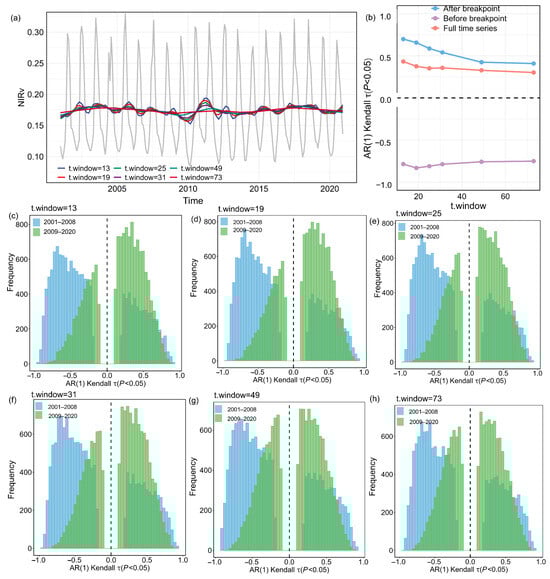
Figure A3.
(a) The detrended NIRv time series for a representative grid box based on t.window is shown (shaded in gray). (b) The mean AR(1) time series before and after the breakpoint, along with the Kendall τ values for the full AR(1) time series. (c–h) Histograms of Kendall τ values for the AR(1) time series before and after the breakpoint.
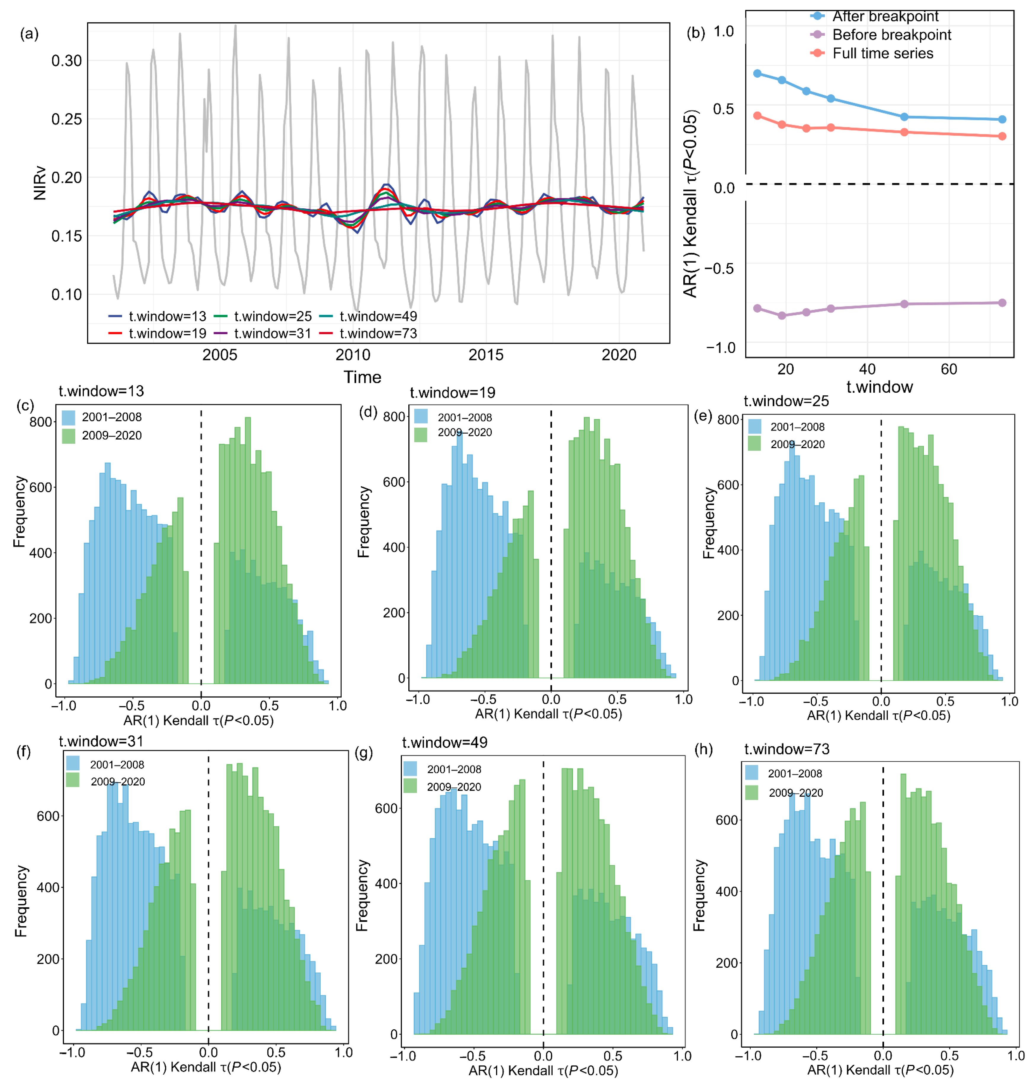
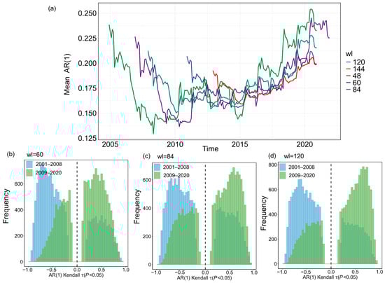
Figure A4.
Robustness of AR(1) to the selection of sliding window length. (a) The mean AR(1) time series is shown for different sliding window lengths (wl), including 4 years (48 months), 5 years (60 months), 7 years (84 months), 10 years (120 months), and 12 years (144 months). (b–d) Histograms of Kendall τ values for individual grid cells under these window length choices, demonstrating that the AR(1) time series consistently shifts from negative to positive tendencies before and after the breakpoint, regardless of the selected window length.
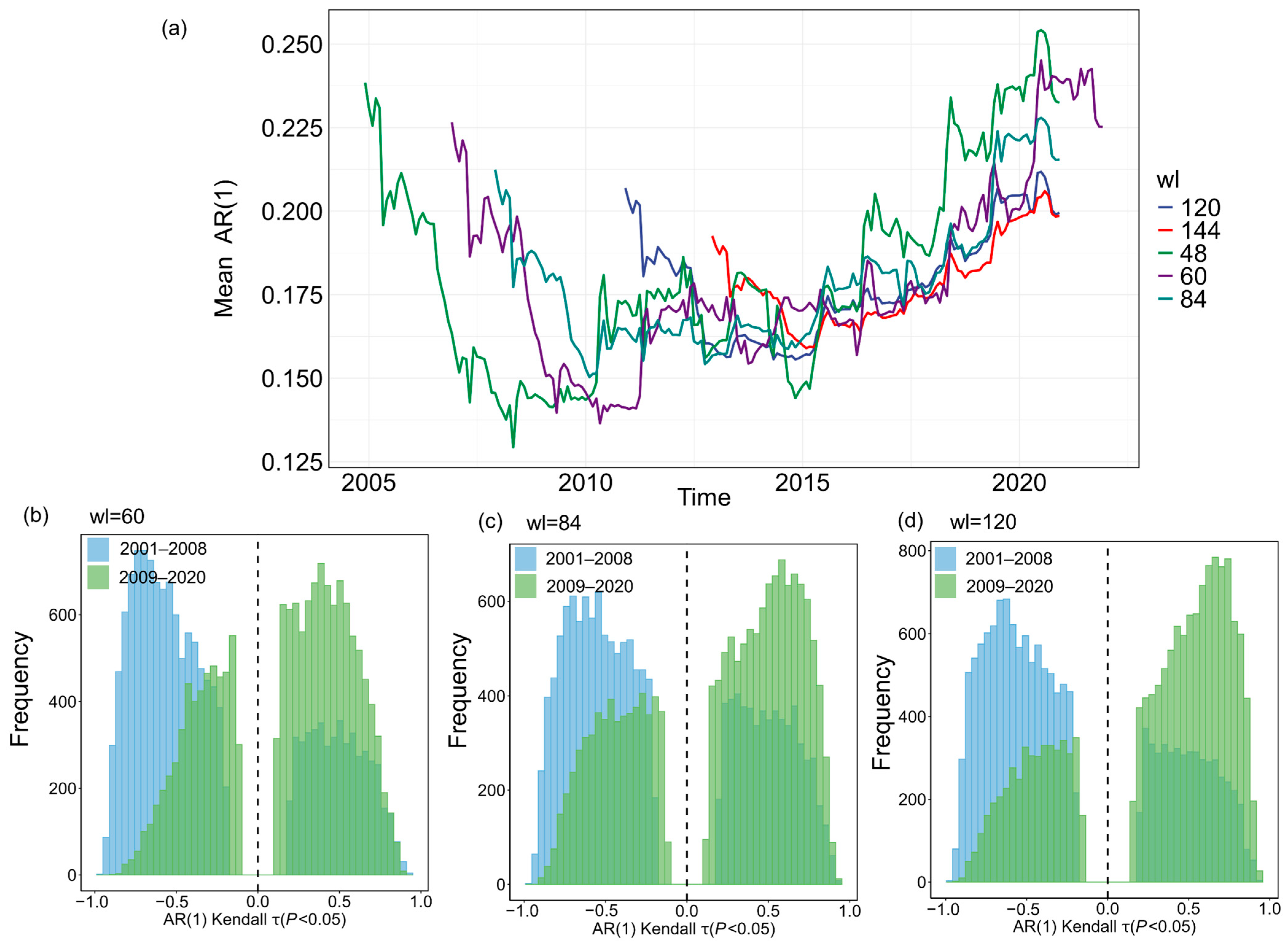
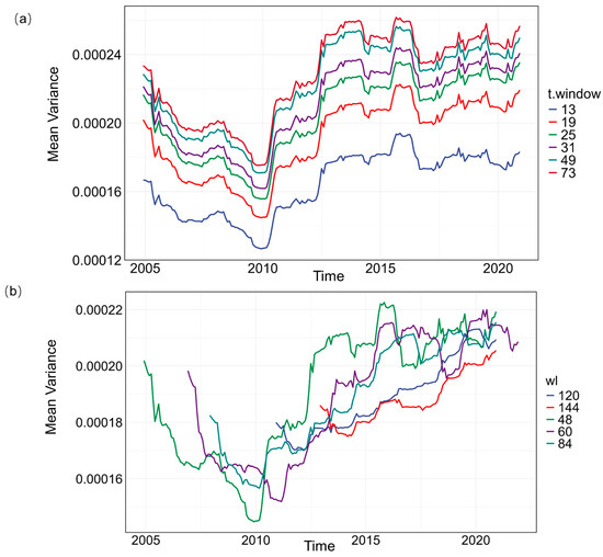
Figure A5.
Select variance as the CSD index, varying t.window and wl, and comparing it with AR(1), as well as comparing it with AR(1). (a) Mean variance time series for different t.window settings. (b) Mean variance time series for different wl settings.
Figure A5.
Select variance as the CSD index, varying t.window and wl, and comparing it with AR(1), as well as comparing it with AR(1). (a) Mean variance time series for different t.window settings. (b) Mean variance time series for different wl settings.

Table A2.
Parameters used for the optimization of the XGBoost regression model.
Table A2.
Parameters used for the optimization of the XGBoost regression model.
| Parameter | Definition | Range |
|---|---|---|
| mtry | The number of features randomly selected for each tree split. | [2, 8] |
| min_n | The minimum number of samples required in a terminal node of the tree. | [5, 10] |
| Tree_depth | The maximum depth allowed for each decision tree. | [1, 20] |
| Learn_rate | The step size used to update the model after each iteration. | [−3, 1] |
| Loss_reduction | The minimum reduction in loss required to make a further split in a tree. | [−3, 0] |
| Sample_prop | The proportion of the dataset used for each tree during training. | [0.8, 1] |
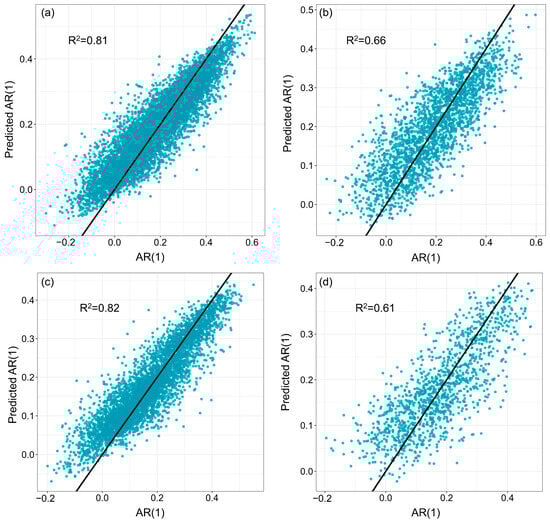
Figure A6.
Performance of the XGBoost models for coniferous and broadleaf forests. (a,b) The coniferous forest model was calibrated using 75% of the records as the training set and validated with the remaining 25% as the test set. (c,d) The broadleaf forest model was calibrated using 75% of the records as the training set and validated with 25% as the test set.
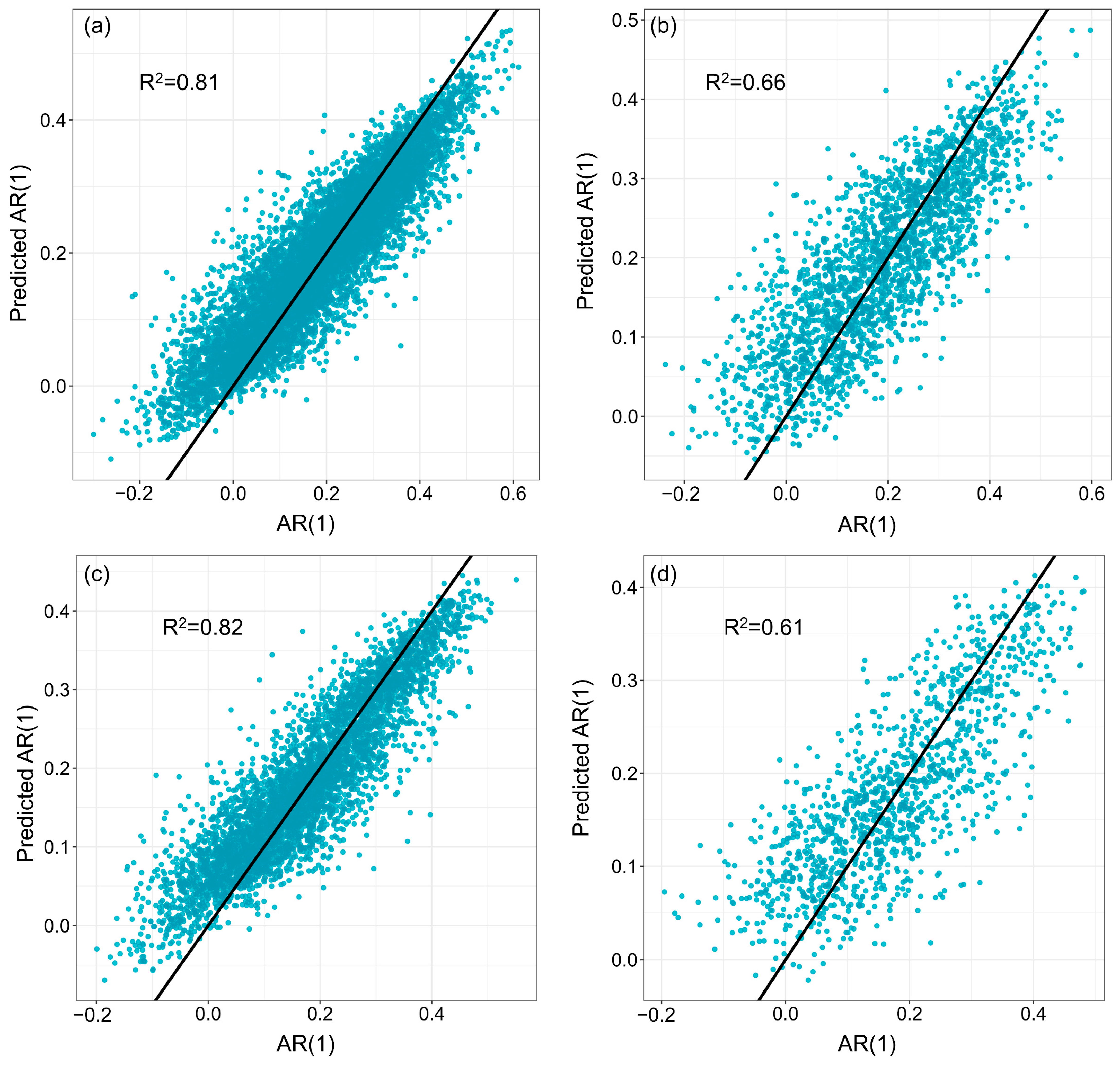
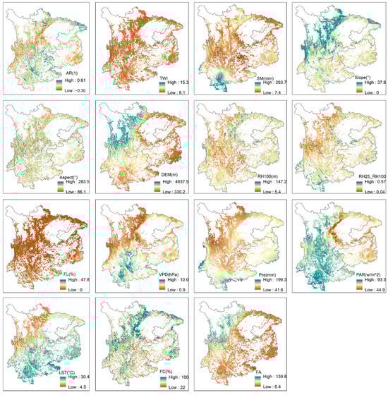
Figure A7.
Spatial distribution patterns of the input variables and the dependent variable in the XGBoost model.
Figure A7.
Spatial distribution patterns of the input variables and the dependent variable in the XGBoost model.
References
- Xiong, Q.; Luo, X.; Liang, P.; Xiao, Y.; Xiao, Q.; Sun, H.; Pan, K.; Wang, L.; Li, L.; Pang, X. Fire from policy, human interventions, or biophysical factors? Temporal–spatial patterns of forest fire in southwestern China. For. Ecol. Manag. 2020, 474, 118381. [Google Scholar] [CrossRef]
- Li, X.; Li, Y.; Chen, A.; Gao, M.; Slette, I.J.; Piao, S. The impact of the 2009/2010 drought on vegetation growth and terrestrial carbon balance in Southwest China. Agric. For. Meteorol. 2019, 269, 239–248. [Google Scholar] [CrossRef]
- Liu, H.; Zhang, M.; Lin, Z.; Xu, X. Spatial heterogeneity of the relationship between vegetation dynamics and climate change and their driving forces at multiple time scales in Southwest China. Agric. For. Meteorol. 2018, 256, 10–21. [Google Scholar] [CrossRef]
- Ding, Z.; Liu, Y.; Wang, L.; Chen, Y.; Yu, P.; Ma, M.; Tang, X. Effects and implications of ecological restoration projects on ecosystem water use efficiency in the karst region of Southwest China. Ecol. Eng. 2021, 170, 106356. [Google Scholar] [CrossRef]
- Liu, L.; Jiang, Y.; Gao, J.; Feng, A.; Jiao, K.; Wu, S.; Zuo, L.; Li, Y.; Yan, R. Concurrent climate extremes and impacts on ecosystems in southwest China. Remote Sens. 2022, 14, 1678. [Google Scholar] [CrossRef]
- Brandt, M.; Yue, Y.; Wigneron, J.P.; Tong, X.; Tian, F.; Jepsen, M.R.; Xiao, X.; Verger, A.; Mialon, A.; Al Yaari, A. Satellite-observed major greening and biomass increase in south China karst during recent decade. Earth’s Future 2018, 6, 1017–1028. [Google Scholar] [CrossRef]
- Wang, Z.; Fu, B.; Wu, X.; Li, Y.; Feng, Y.; Wang, S.; Wei, F.; Zhang, L. Vegetation resilience does not increase consistently with greening in China’s Loess Plateau. Commun. Earth Environ. 2023, 4, 336. [Google Scholar] [CrossRef]
- Forzieri, G.; Dakos, V.; McDowell, N.G.; Ramdane, A.; Cescatti, A. Emerging signals of declining forest resilience under climate change. Nature 2022, 608, 534–539. [Google Scholar] [CrossRef]
- Hu, Y.; Wei, F.; Fu, B.; Wang, S.; Zhang, W.; Zhang, Y. Changes and influencing factors of ecosystem resilience in China. Environ. Res. Lett. 2023, 18, 94012. [Google Scholar] [CrossRef]
- Holling, C.S. Resilience and Stability of Ecological Systems; International Institute for Applied Systems Analysis: Laxenburg, Austria, 1973. [Google Scholar]
- Scheffer, M.; Bascompte, J.; Brock, W.A.; Brovkin, V.; Carpenter, S.R.; Dakos, V.; Held, H.; Van Nes, E.H.; Rietkerk, M.; Sugihara, G. Early-warning signals for critical transitions. Nature 2009, 461, 53–59. [Google Scholar] [CrossRef]
- Hirota, M.; Holmgren, M.; Van Nes, E.H.; Scheffer, M. Global resilience of tropical forest and savanna to critical transitions. Science 2011, 334, 232–235. [Google Scholar] [CrossRef] [PubMed]
- Scheffer, M.; Carpenter, S.; Foley, J.A.; Folke, C.; Walker, B. Catastrophic shifts in ecosystems. Nature 2001, 413, 591–596. [Google Scholar] [CrossRef]
- Seidl, R.; Thom, D.; Kautz, M.; Martin-Benito, D.; Peltoniemi, M.; Vacchiano, G.; Wild, J.; Ascoli, D.; Petr, M.; Honkaniemi, J. Forest disturbances under climate change. Nat. Clim. Change 2017, 7, 395–402. [Google Scholar] [CrossRef]
- Lloret, F.; Keeling, E.G.; Sala, A. Components of tree resilience: Effects of successive low-growth episodes in old ponderosa pine forests. Oikos 2011, 120, 1909–1920. [Google Scholar] [CrossRef]
- Bottero, A.; Forrester, D.I.; Cailleret, M.; Kohnle, U.; Gessler, A.; Michel, D.; Bose, A.K.; Bauhus, J.; Bugmann, H.; Cuntz, M.; et al. Growth resistance and resilience of mixed silver fir and Norway spruce forests in central Europe: Contrasting responses to mild and severe droughts. Glob. Change Biol. 2021, 27, 4403–4419. [Google Scholar] [CrossRef] [PubMed]
- Zas, R.; Sampedro, L.; Solla, A.; Vivas, M.; Lombardero, M.J.; Alia, R.; Rozas, V. Dendroecology in common gardens: Population differentiation and plasticity in resistance, recovery and resilience to extreme drought events in Pinus pinaster. Agric. For. Meteorol. 2020, 291, 108060. [Google Scholar] [CrossRef]
- Fang, O.; Zhang, Q. Tree resilience to drought increases in the Tibetan Plateau. Glob. Change Biol. 2019, 25, 245–253. [Google Scholar] [CrossRef]
- Isbell, F.; Craven, D.; Connolly, J.; Loreau, M.; Schmid, B.; Beierkuhnlein, C.; Bezemer, T.M.; Bonin, C.; Bruelheide, H.; de Luca, E.; et al. Biodiversity increases the resistance of ecosystem productivity to climate extremes. Nature 2015, 526, 263–574. [Google Scholar] [CrossRef]
- Piao, S.; Wang, X.; Park, T.; Chen, C.; Lian, X.; He, Y.; Bjerke, J.W.; Chen, A.; Ciais, P.; Tømmervik, H. Characteristics, drivers and feedbacks of global greening. Nat. Rev. Earth Environ. 2020, 1, 14–27. [Google Scholar] [CrossRef]
- Boulton, C.A.; Lenton, T.M.; Boers, N. Pronounced loss of Amazon rainforest resilience since the early 2000s. Nat. Clim. Change 2022, 12, 271–278. [Google Scholar] [CrossRef]
- Smith, T.; Traxl, D.; Boers, N. Empirical evidence for recent global shifts in vegetation resilience. Nat. Clim. Change 2022, 12, 477–484. [Google Scholar] [CrossRef]
- Wang, H.; Ciais, P.; Sitch, S.; Green, J.K.; Tao, S.; Fu, Z.; Albergel, C.; Bastos, A.; Wang, M.; Fawcett, D. Anthropogenic disturbance exacerbates resilience loss in the Amazon rainforests. Glob. Change Biol. 2024, 30, e17006. [Google Scholar] [CrossRef]
- Chen, J.; Wang, S.; Shi, H.; Chen, B.; Wang, J.; Zheng, C.; Zhu, K. Radiation and temperature dominate the spatiotemporal variability in resilience of subtropical evergreen forests in China. Front. For. Glob. Change 2023, 6, 1166481. [Google Scholar] [CrossRef]
- Van Passel, J.; Bernardino, P.N.; Lhermitte, S.; Rius, B.F.; Hirota, M.; Conradi, T.; de Keersmaecker, W.; Van Meerbeek, K.; Somers, B. Critical slowing down of the Amazon forest after increased drought occurrence. Proc. Natl. Acad. Sci. USA 2024, 121, e1978043175. [Google Scholar] [CrossRef] [PubMed]
- Wang, L.; Chen, W.; Haung, G.; Wang, T.; Wang, Q.; Su, X.; Ren, Z.; Chotamonsak, C.; Limsakul, A.; Torsri, K. Characteristics of super drought in Southwest China and the associated compounding effect of multiscalar anomalies. Sci. China Earth Sci. 2024, 67, 2084–2102. [Google Scholar] [CrossRef]
- Zhang, L.; Xiao, J.; Li, J.; Wang, K.; Lei, L.; Guo, H. The 2010 spring drought reduced primary productivity in southwestern China. Environ. Res. Lett. 2012, 7, 45706. [Google Scholar] [CrossRef]
- Corlett, R.T. The impacts of droughts in tropical forests. Trends Plant Sci. 2016, 21, 584–593. [Google Scholar] [CrossRef]
- Feldpausch, T.R.; Phillips, O.L.; Brienen, R.; Gloor, E.; Lloyd, J.; Lopez Gonzalez, G.; Monteagudo Mendoza, A.; Malhi, Y.; Alarcón, A.; Álvarez Dávila, E. Amazon forest response to repeated droughts. Glob. Biogeochem. Cycles 2016, 30, 964–982. [Google Scholar] [CrossRef]
- Hu, Y.; Xiang, W.; Schäfer, K.V.; Lei, P.; Deng, X.; Forrester, D.I.; Fang, X.; Zeng, Y.; Ouyang, S.; Chen, L. Photosynthetic and hydraulic traits influence forest resistance and resilience to drought stress across different biomes. Sci. Total Environ. 2022, 828, 154517. [Google Scholar] [CrossRef]
- Zeng, Z.; Wu, W.; Penuelas, J.; Li, Y.; Jiao, W.; Li, Z.; Ren, X.; Wang, K.; Ge, Q. Increased risk of flash droughts with raised concurrent hot and dry extremes under global warming. npj Clim. Atmos. Sci. 2023, 6, 134. [Google Scholar] [CrossRef]
- Smith, T.; Boers, N. Reliability of vegetation resilience estimates depends on biomass density. Nat. Ecol. Evol. 2023, 7, 1799–1808. [Google Scholar] [CrossRef]
- Zhu, L.; Zhang, J.; Camarero, J.J.; Cooper, D.J.; Cherubini, P.; Yuan, D.; Wang, X. Drivers and spatiotemporal patterns of post-drought growth resilience of four temperate broad-leaved trees. Agric. For. Meteorol. 2023, 342, 109741. [Google Scholar] [CrossRef]
- Shan, R.; Feng, G.; Lin, Y.; Ma, Z. Temporal stability of forest productivity declines over stand age at multiple spatial scales. Nat. Commun. 2025, 16, 2745. [Google Scholar] [CrossRef] [PubMed]
- Liu, Y.; Xiao, P.; Zhang, X.; Liu, H.; Chen, S.; Jia, Y. Accelerated Decline in Vegetation Resilience on the Tibetan Plateau. Land Degrad. Dev. 2025, 36, 295–306. [Google Scholar] [CrossRef]
- Shao, H.; Zhang, Y.; Yu, Z.; Gu, F.; Peng, Z. The resilience of vegetation to the 2009/2010 extreme drought in southwest China. Forests 2022, 13, 851. [Google Scholar] [CrossRef]
- Lu, Q.; Zhang, Y.; Song, B.; Shao, H.; Tian, X.; Liu, S. The responses of ecological indicators to compound extreme climate indices in Southwestern China. Ecol. Indic. 2023, 157, 111253. [Google Scholar] [CrossRef]
- Schaaf, C.; Wang, Z. MODIS/Terra+Aqua BRDF/Albedo Nadir BRDF-Adjusted Ref Daily L3 Global 0.05Deg CMG V061. 2021. Distributed by NASA EOSDIS Land Processes Distributed Active Archive Center. Available online: https://doi.org/10.5067/MODIS/MCD43C4.061 (accessed on 27 March 2025).
- Rocha, J.C. Ecosystems are showing symptoms of resilience loss. Environ. Res. Lett. 2022, 17, 65013. [Google Scholar] [CrossRef]
- Badgley, G.; Field, C.B.; Berry, J.A. Canopy near-infrared reflectance and terrestrial photosynthesis. Sci. Adv. 2017, 3, e1602244. [Google Scholar] [CrossRef]
- Li, X.; Xiao, J. A global, 0.05-degree product of solar-induced chlorophyll fluorescence derived from OCO-2, MODIS, and reanalysis data. Remote Sens. 2019, 11, 517. [Google Scholar] [CrossRef]
- Hansen, M.C.; Potapov, P.V.; Moore, R.; Hancher, M.; Turubanova, S.A.; Tyukavina, A.; Thau, D.; Stehman, S.V.; Goetz, S.J.; Loveland, T.R. High-resolution global maps of 21st-century forest cover change. Science 2013, 342, 850–853. [Google Scholar] [CrossRef]
- Yang, H.; Ciais, P.; Wigneron, J.; Chave, J.; Cartus, O.; Chen, X.; Fan, L.; Green, J.K.; Huang, Y.; Joetzjer, E. Climatic and biotic factors influencing regional declines and recovery of tropical forest biomass from the 2015/16 El Niño. Proc. Natl. Acad. Sci. USA 2022, 119, e2101388119. [Google Scholar] [CrossRef] [PubMed]
- Besnard, S.; Koirala, S.; Santoro, M.; Weber, U.; Nelson, J.; Gütter, J.; Herault, B.; Kassi, J.; N’Guessan, A.; Neigh, C. Mapping global forest age from forest inventories, biomass and climate data. Earth Syst. Sci. Data Discuss. 2021, 13, 4881–4896. [Google Scholar] [CrossRef]
- Vicente-Serrano, S.M.; Beguería, S.; López-Moreno, J.I.; Angulo, M.; El Kenawy, A. A new global 0.5 gridded dataset (1901–2006) of a multiscalar drought index: Comparison with current drought index datasets based on the Palmer Drought Severity Index. J. Hydrometeorol. 2010, 11, 1033–1043. [Google Scholar] [CrossRef]
- Yu, H.; Wang, L.; Zhang, J.; Chen, Y. A global drought-aridity index: The spatiotemporal standardized precipitation evapotranspiration index. Ecol. Indic. 2023, 153, 110484. [Google Scholar] [CrossRef]
- Buck, A.L. New equations for computing vapor pressure and enhancement factor. J. Appl. Meteorol. 1981, 20, 1527–1532. [Google Scholar] [CrossRef]
- Wan, Z.; Hook, S.; Hulley, G. MOD11A1 MODIS/Terra Land Surface Temperature/Emissivity Daily L3 Global 1km SIN Grid V006; NASA EOSDIS Land Processes Distributed Active Archive Center: Sioux Falls, SD, USA, 2015.
- Abatzoglou, J.T.; Dobrowski, S.Z.; Parks, S.A.; Hegewisch, K.C. TerraClimate, a high-resolution global dataset of monthly climate and climatic water balance from 1958–2015. Sci. Data 2018, 5, 170191. [Google Scholar] [CrossRef]
- Wissel, C. A universal law of the characteristic return time near thresholds. Oecologia 1984, 65, 101–107. [Google Scholar] [CrossRef] [PubMed]
- Biggs, R.; Carpenter, S.R.; Brock, W.A. Turning back from the brink: Detecting an impending regime shift in time to avert it. Proc. Natl. Acad. Sci. USA 2009, 106, 826–831. [Google Scholar] [CrossRef]
- Verbesselt, J.; Umlauf, N.; Hirota, M.; Holmgren, M.; Van Nes, E.H.; Herold, M.; Zeileis, A.; Scheffer, M. Remotely sensed resilience of tropical forests. Nat. Clim. Change 2016, 6, 1028–1031. [Google Scholar] [CrossRef]
- Liu, Y.; Kumar, M.; Katul, G.G.; Porporato, A. Reduced resilience as an early warning signal of forest mortality. Nat. Clim. Change 2019, 9, 880–885. [Google Scholar] [CrossRef]
- Team, R.C. R: A Language and Environment for Statistical Computing. R Foundation for Statistical Computing (Version 4.3.2). 2023. Available online: https://www.R-project.org/ (accessed on 1 January 2023).
- He, J.; Shi, Y.; Xu, L.; Lu, Z.; Feng, M.; Tang, J.; Guo, X. Exploring the scale effect of urban thermal environment through XGBoost model. Sustain. Cities Soc. 2024, 114, 105763. [Google Scholar] [CrossRef]
- Yuan, Y.; Guo, W.; Tang, S.; Zhang, J. Effects of patterns of urban green-blue landscape on carbon sequestration using XGBoost-SHAP model. J. Clean Prod. 2024, 476, 143640. [Google Scholar] [CrossRef]
- Li, Z. Extracting spatial effects from machine learning model using local interpretation method: An example of SHAP and XGBoost. Comput. Environ. Urban Syst. 2022, 96, 101845. [Google Scholar] [CrossRef]
- Zhou, B.; Chen, G.; Yu, H.; Zhao, J.; Yin, Y. Revealing the Nonlinear Impact of Human Activities and Climate Change on Ecosystem Services in the Karst Region of Southeastern Yunnan Using the XGBoost–SHAP Model. Forests 2024, 15, 1420. [Google Scholar] [CrossRef]
- Ekanayake, I.U.; Meddage, D.; Rathnayake, U. A novel approach to explain the black-box nature of machine learning in compressive strength predictions of concrete using Shapley additive explanations (SHAP). Case Stud. Constr. Mater. 2022, 16, e01059. [Google Scholar] [CrossRef]
- Lundberg, S.M.; Erion, G.; Chen, H.; DeGrave, A.; Prutkin, J.M.; Nair, B.; Katz, R.; Himmelfarb, J.; Bansal, N.; Lee, S. From local explanations to global understanding with explainable AI for trees. Nat. Mach. Intell. 2020, 2, 56–67. [Google Scholar] [CrossRef] [PubMed]
- Lundberg, S.M.; Lee, S. A unified approach to interpreting model predictions. Adv. Neural Inf. Process. Syst. 2017, 30, 4768–4777. [Google Scholar]
- Temenos, A.; Tzortzis, I.N.; Kaselimi, M.; Rallis, I.; Doulamis, A.; Doulamis, N. Novel insights in spatial epidemiology utilizing explainable AI (XAI) and remote sensing. Remote Sens. 2022, 14, 3074. [Google Scholar] [CrossRef]
- Fong, Y.; Huang, Y.; Gilbert, P.B.; Permar, S.R. chngpt: Threshold regression model estimation and inference. BMC Bioinform. 2017, 18, 454. [Google Scholar] [CrossRef]
- Taneda, H.; Funayama-Noguchi, S.; Mayr, S.; Goto, S. Elevational adaptation of morphological and anatomical traits by Sakhalin fir (Abies sachalinensis). Trees 2020, 34, 507–520. [Google Scholar] [CrossRef]
- Li, X.; Liang, E.; Camarero, J.J.; Rossi, S.; Zhang, J.; Zhu, H.; Fu, Y.; Sun, J.; Wang, T.; Piao, S. Warming-induced phenological mismatch between trees and shrubs explains high-elevation forest expansion. Natl. Sci. Rev. 2023, 10, nwad182. [Google Scholar] [CrossRef] [PubMed]
- Shi, S.; Liu, G.; Li, Z.; Ye, X. Elevation-dependent growth trends of forests as affected by climate warming in the southeastern Tibetan Plateau. For. Ecol. Manag. 2021, 498, 119551. [Google Scholar] [CrossRef]
- So, K.; Rogers, C.A.; Li, Y.; Arain, M.A.; Gonsamo, A. Retention forestry as a climate solution: Assessing biomass, soil carbon and albedo impacts in a northern temperate coniferous forest. Sci. Total Environ. 2024, 947, 174680. [Google Scholar] [CrossRef]
- Zhao, J.; Yue, C.; Wang, J.; Hantson, S.; Wang, X.; He, B.; Li, G.; Wang, L.; Zhao, H.; Luyssaert, S. Forest fire size amplifies postfire land surface warming. Nature 2024, 633, 828–834. [Google Scholar] [CrossRef] [PubMed]
- Luo, X.; Keenan, T.F. Global evidence for the acclimation of ecosystem photosynthesis to light. Nat. Ecol. Evol. 2020, 4, 1351–1357. [Google Scholar] [CrossRef]
- Perron, N.; Baltzer, J.L.; Detto, M.; Nehemy, M.; Spence, C.; Hould Gosselin, G.; Alcock, H.; Hadiwijaya, B.; Laroque, C.P.; Sonnentag, O. Radiation, air temperature, and soil water availability drive tree water deficit across temporal scales in Canada’s western boreal forest. Geophys. Res. Lett. 2024, 51, e2023GL107477. [Google Scholar] [CrossRef]
- Grossiord, C.; Sevanto, S.; Borrego, I.; Chan, A.M.; Collins, A.D.; Dickman, L.T.; Hudson, P.J.; McBranch, N.; Michaletz, S.T.; Pockman, W.T. Tree water dynamics in a drying and warming world. Plant Cell Environ. 2017, 40, 1861–1873. [Google Scholar] [CrossRef]
- Mirabel, A.; Girardin, M.P.; Metsaranta, J.; Way, D.; Reich, P.B. Increasing atmospheric dryness reduces boreal forest tree growth. Nat. Commun. 2023, 14, 6901. [Google Scholar] [CrossRef]
- Shekhar, A.; Hörtnagl, L.; Buchmann, N.; Gharun, M. Long-term changes in forest response to extreme atmospheric dryness. Glob. Change Biol. 2023, 29, 5379–5396. [Google Scholar] [CrossRef]
- Crous, K.Y.; Uddling, J.; De Kauwe, M.G. Temperature responses of photosynthesis and respiration in evergreen trees from boreal to tropical latitudes. New Phytol. 2022, 234, 353–374. [Google Scholar] [CrossRef]
- Yao, Y.; Liu, Y.; Zhou, S.; Song, J.; Fu, B. Soil moisture determines the recovery time of ecosystems from drought. Glob. Change Biol. 2023, 29, 3562–3574. [Google Scholar] [CrossRef] [PubMed]
- Larson, J.; Wallerman, J.; Peichl, M.; Laudon, H. Soil moisture controls the partitioning of carbon stocks across a managed boreal forest landscape. Sci. Rep. 2023, 13, 14909. [Google Scholar] [CrossRef]
- Matin, M.A.; Chitale, V.S.; Murthy, M.S.; Uddin, K.; Bajracharya, B.; Pradhan, S. Understanding forest fire patterns and risk in Nepal using remote sensing, geographic information system and historical fire data. Int. J. Wildland Fire 2017, 26, 276–286. [Google Scholar] [CrossRef]
- Çolak, E.; Sunar, F. Investigating the usefulness of satellite-retrieved land surface temperature (LST) in pre-and post-fire spatial analysis. Earth Sci. Inform. 2023, 16, 945–963. [Google Scholar] [CrossRef]
- Wang, J.; Hong, R.; Ma, C.; Zhu, X.; Xu, S.; Tang, Y.; Li, X.; Yan, X.; Wang, L.; Wang, Q. Effects of Prescribed Burning on Surface Dead Fuel and Potential Fire Behavior in Pinus yunnanensis in Central Yunnan Province, China. Forests 2023, 14, 1915. [Google Scholar] [CrossRef]
- Dannenberg, M.P.; Wise, E.K.; Smith, W.K. Reduced tree growth in the semiarid United States due to asymmetric responses to intensifying precipitation extremes. Sci. Adv. 2019, 5, eaaw0667. [Google Scholar] [CrossRef]
- Wei, X.; Zhou, Q.; Cai, M.; Wang, Y. Effects of vegetation restoration on regional soil moisture content in the humid karst areas—A case study of Southwest China. Water 2021, 13, 321. [Google Scholar] [CrossRef]
- Bai, P.; Liu, X.; Zhang, Y.; Liu, C. Assessing the impacts of vegetation greenness change on evapotranspiration and water yield in China. Water Resour. Res. 2020, 56, e2019WR027019. [Google Scholar] [CrossRef]
- Zhou, Q.; Keith, D.M.; Zhou, X.; Cai, M.; Cui, X.; Wei, X.; Luo, Y. Comparing the water-holding characteristics of broadleaved, coniferous, and mixed forest litter layers in a Karst Region. Mt. Res. Dev. 2018, 38, 220–229. [Google Scholar] [CrossRef]
- Hossain, M.L.; Li, J. NDVI-based vegetation dynamics and its resistance and resilience to different intensities of climatic events. Glob. Ecol. Conserv. 2021, 30, e01768. [Google Scholar] [CrossRef]
- Zhang, P.; Jiao, L.; Wei, M.; Wu, X.; Du, D.; Xue, R. Drought timing and severity affect radial growth of Picea crassifolia at different elevations in the western Qilian Mountains. Int. J. Biometeorol. 2022, 66, 2449–2462. [Google Scholar] [CrossRef] [PubMed]
- Hossain, M.L.; Li, J.; Lai, Y.; Beierkuhnlein, C. Long-term evidence of differential resistance and resilience of grassland ecosystems to extreme climate events. Environ. Monit. Assess. 2023, 195, 734. [Google Scholar] [CrossRef] [PubMed]
- Dakos, V.; Carpenter, S.R.; van Nes, E.H.; Scheffer, M. Resilience indicators: Prospects and limitations for early warnings of regime shifts. Philos. Trans. R. Soc. B Biol. Sci. 2015, 370, 20130263. [Google Scholar] [CrossRef]
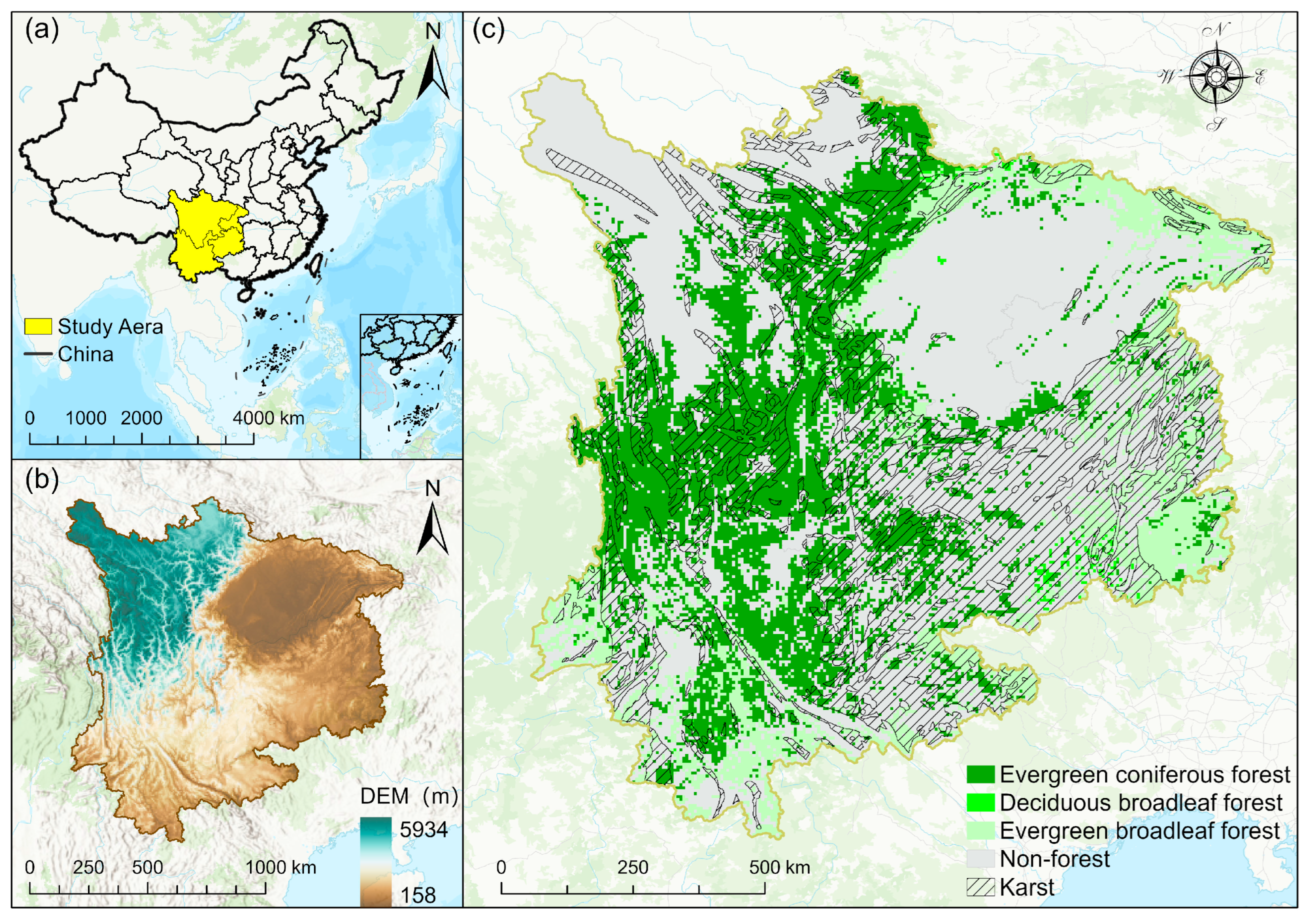
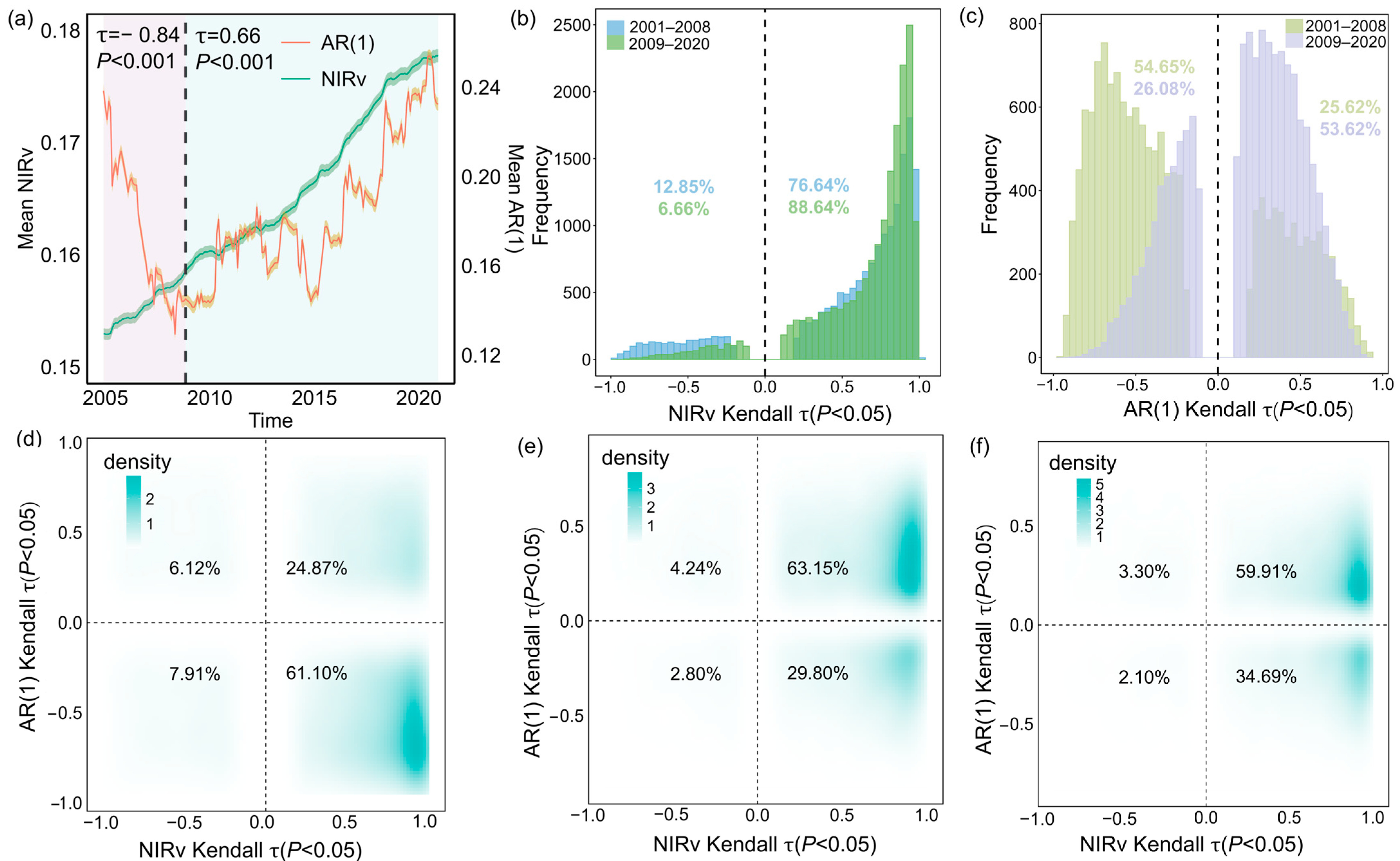
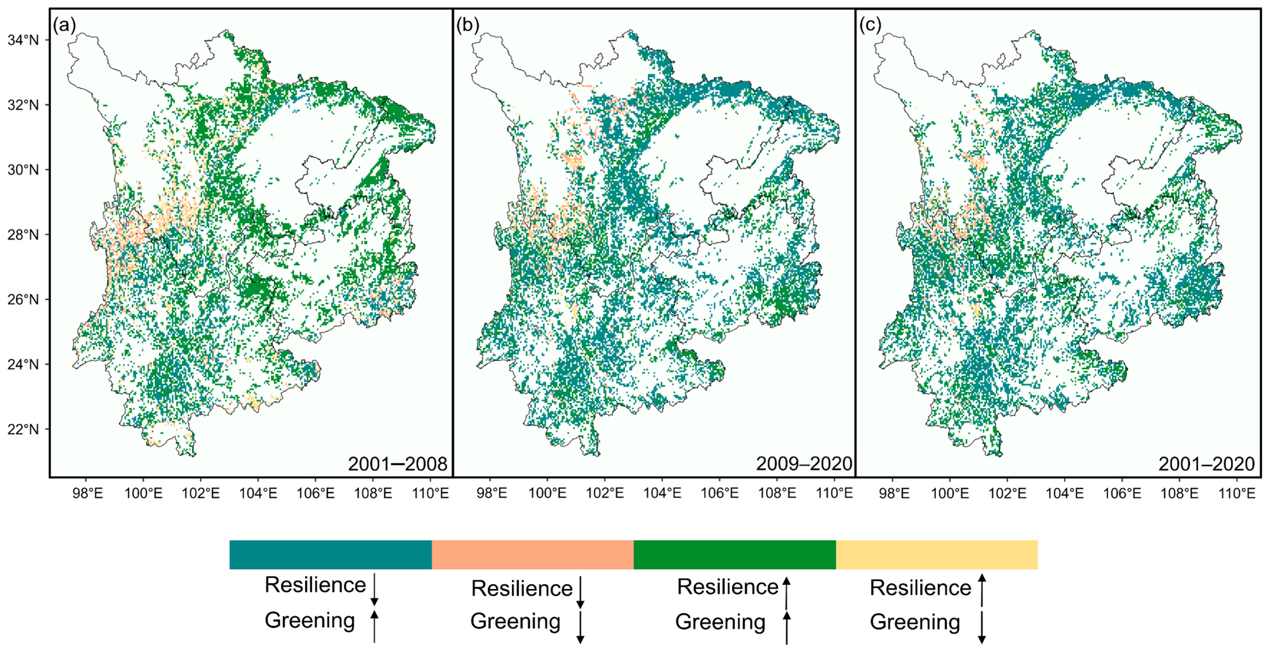
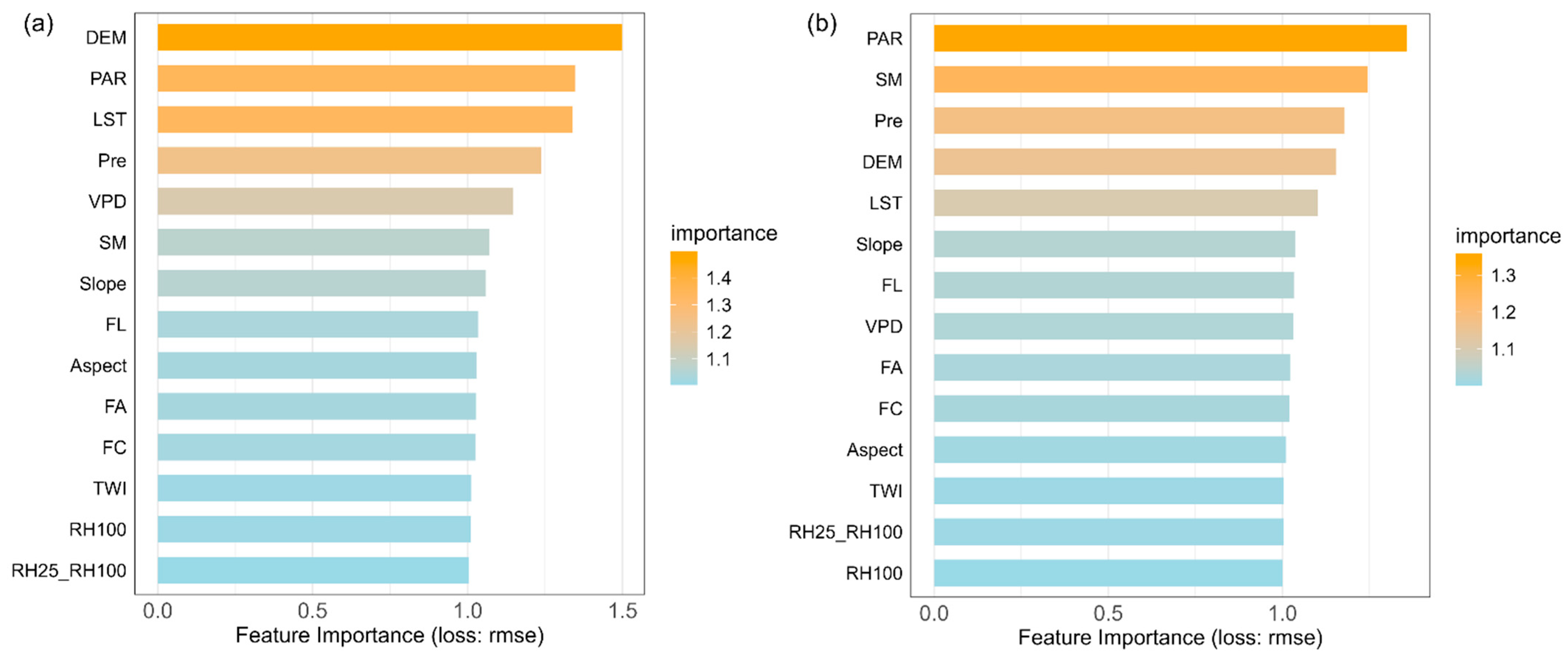
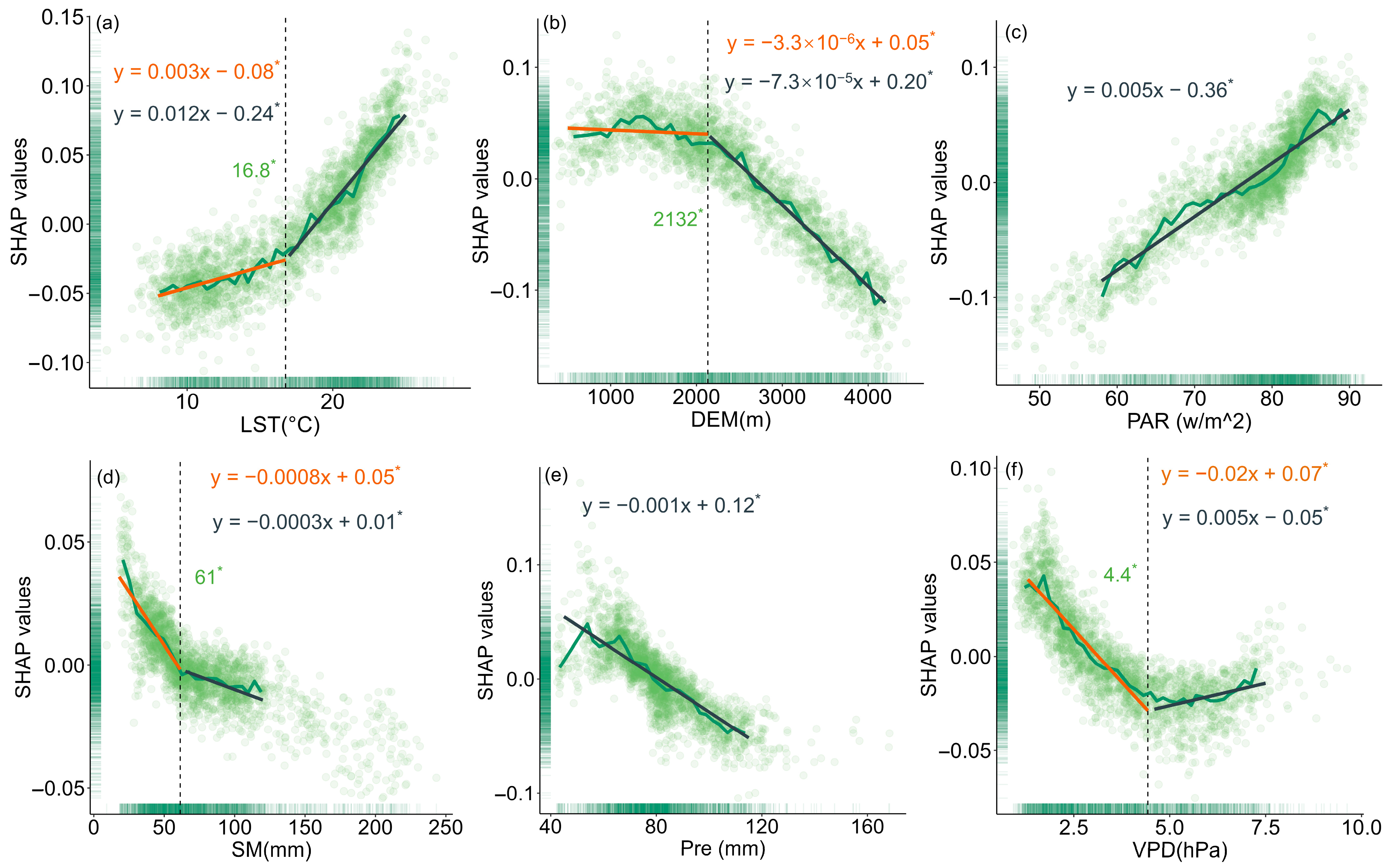
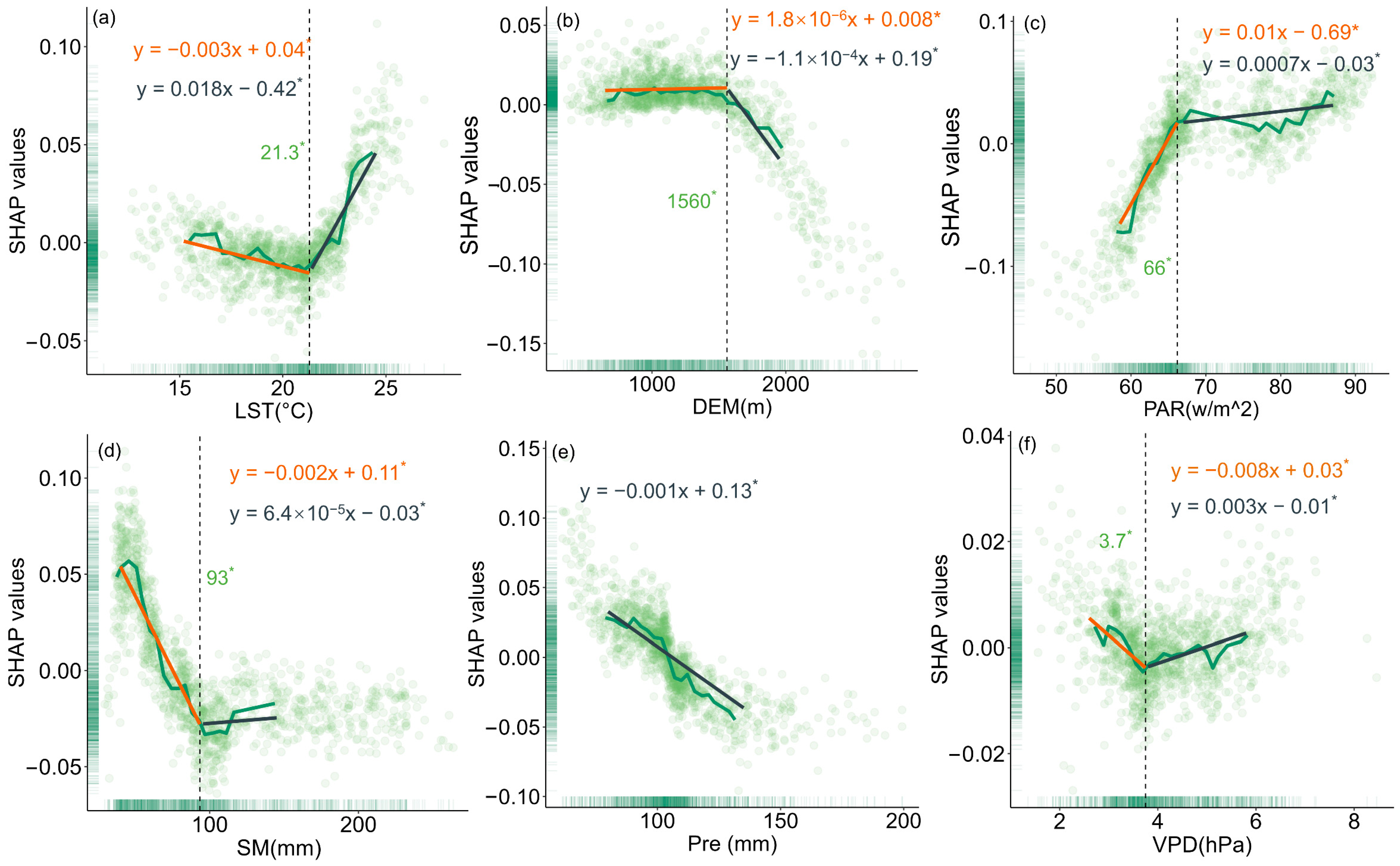
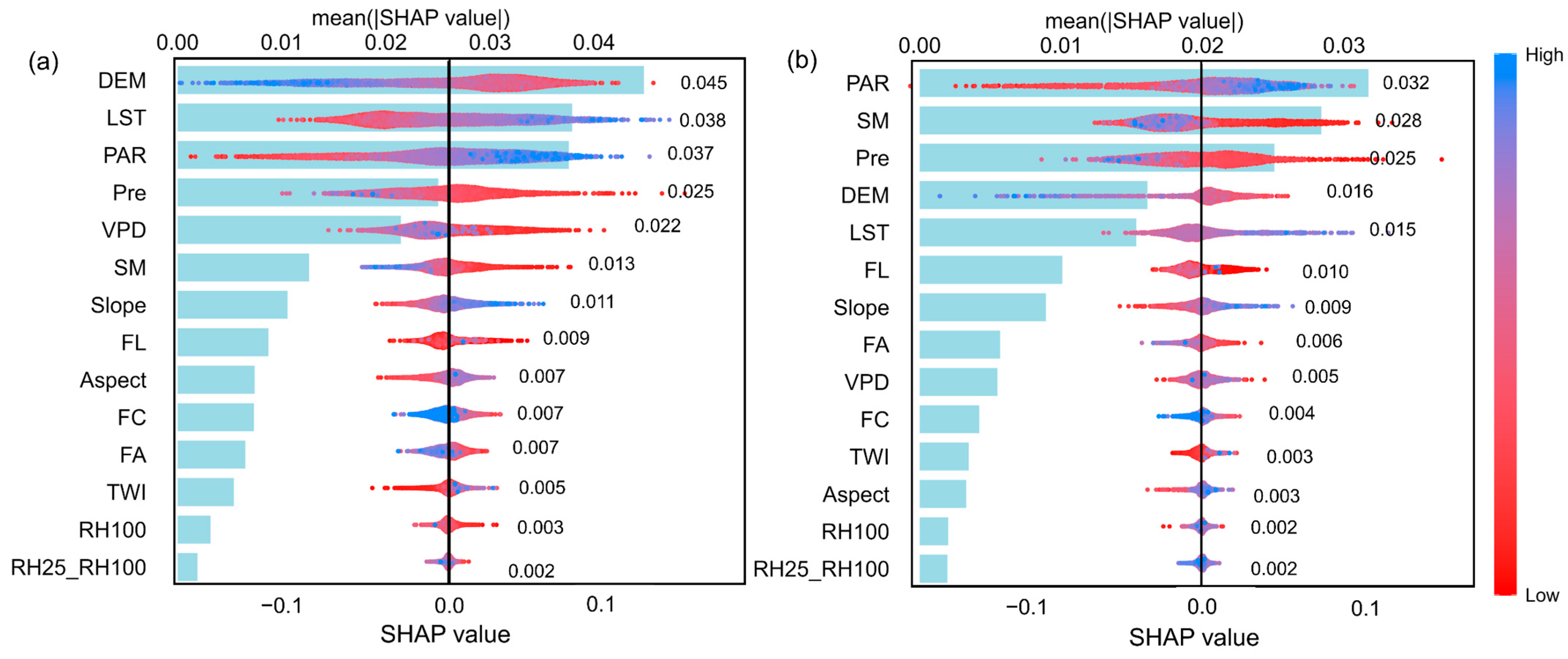
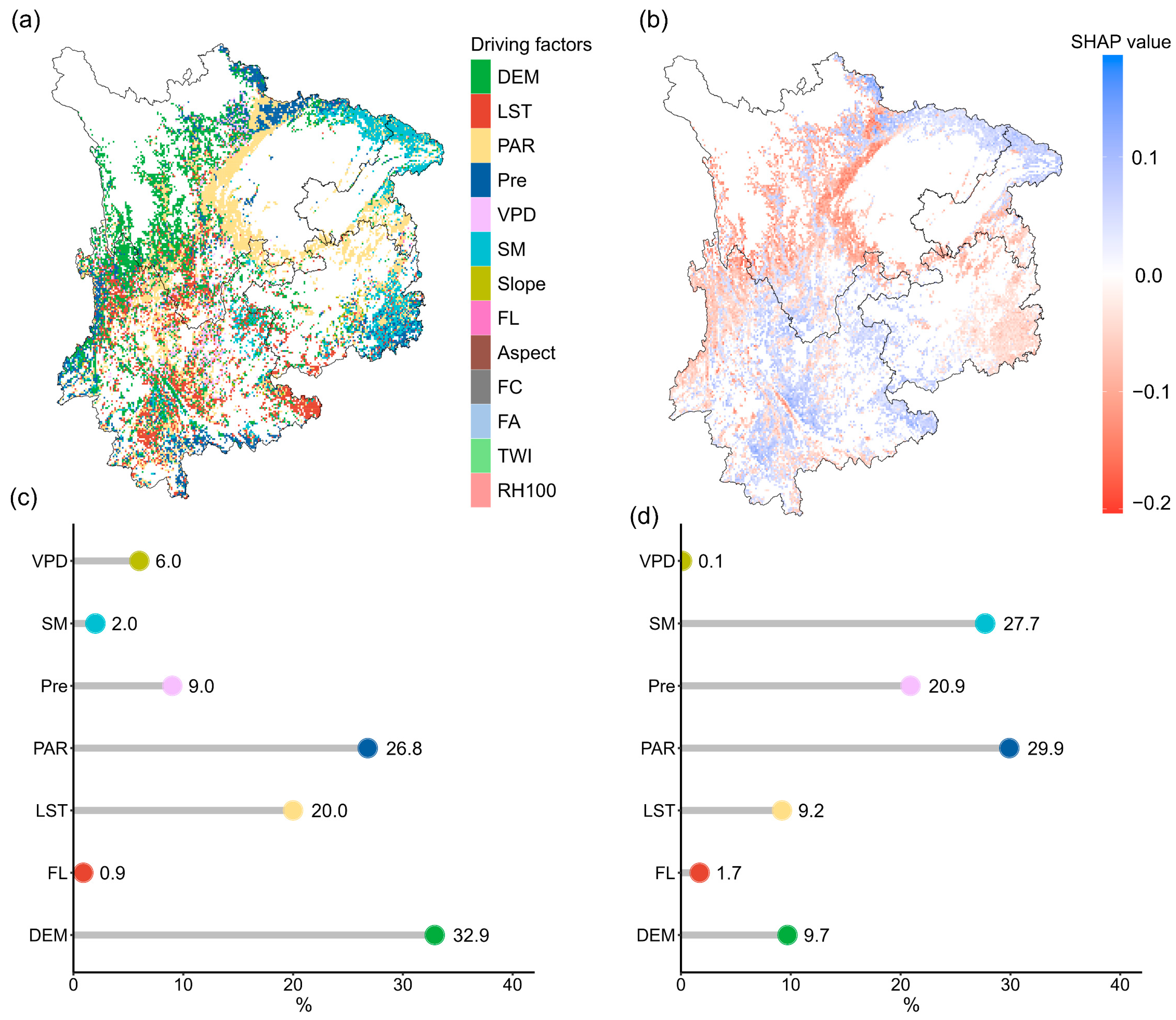
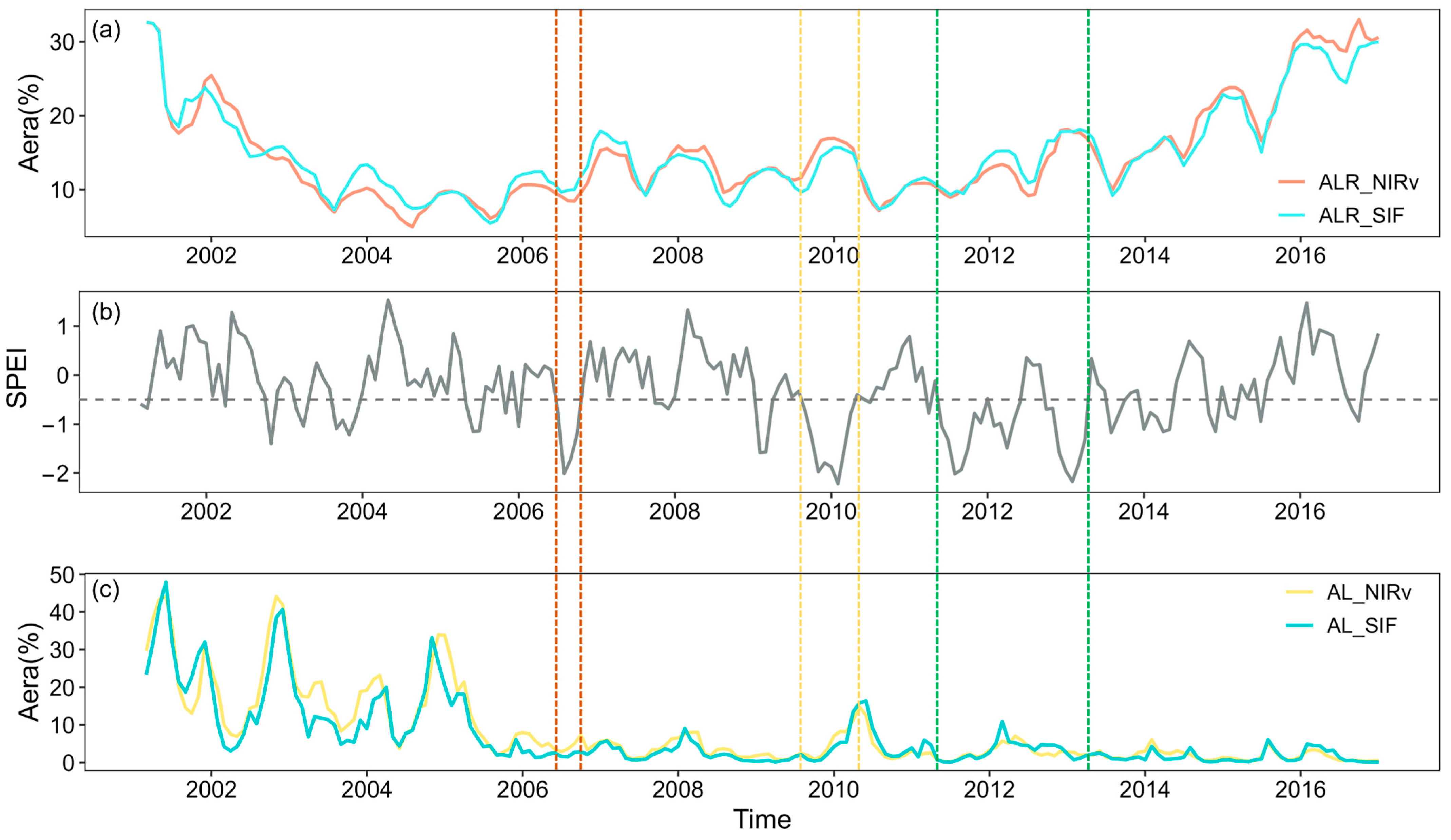

Disclaimer/Publisher’s Note: The statements, opinions and data contained in all publications are solely those of the individual author(s) and contributor(s) and not of MDPI and/or the editor(s). MDPI and/or the editor(s) disclaim responsibility for any injury to people or property resulting from any ideas, methods, instructions or products referred to in the content. |
© 2025 by the authors. Licensee MDPI, Basel, Switzerland. This article is an open access article distributed under the terms and conditions of the Creative Commons Attribution (CC BY) license (https://creativecommons.org/licenses/by/4.0/).