Abstract
Accurate, detailed, and up-to-date tree species distribution information is essential for effective forest management and environmental research. However, existing tree species maps face limitations in resolution and update cycle, making it difficult to meet modern demands. To overcome these limitations, this study proposes a novel framework that utilizes existing medium-resolution national tree species maps as ‘weak labels’ and fuses multi-temporal Sentinel-2 and PlanetScope satellite imagery data. Specifically, a super-resolution (SR) technique, using PlanetScope imagery as a reference, was first applied to Sentinel-2 data to enhance its resolution to 2.5 m. Then, these enhanced Sentinel-2 bands were combined with PlanetScope bands to construct the final multi-spectral, multi-temporal input data. Deep learning (DL) model training data was constructed by strategically sampling information-rich pixels from the national tree species map. Applying the proposed methodology to Sobaeksan and Jirisan National Parks in South Korea, the performance of various machine learning (ML) and deep learning (DL) models was compared, including traditional ML (linear regression, random forest) and DL architectures (multilayer perceptron (MLP), spectral encoder block (SEB)—linear, and SEB-transformer). The MLP model demonstrated optimal performance, achieving over 85% overall accuracy (OA) and more than 81% accuracy in classifying spectrally similar and difficult-to-distinguish species, specifically Quercus mongolica (QM) and Quercus variabilis (QV). Furthermore, while spectral and temporal information were confirmed to contribute significantly to tree species classification, the contribution of spatial (texture) information was experimentally found to be limited at the 2.5 m resolution level. This study presents a practical method for creating high-resolution tree species maps scalable to the national level by fusing existing tree species maps with Sentinel-2 and PlanetScope imagery without requiring costly separate field surveys. Its significance lies in establishing a foundation that can contribute to various fields such as forest resource management, biodiversity conservation, and climate change research.
1. Introduction
Accurate and up-to-date tree species distribution information is essential foundational data for effective modern forest management and environmental research. This information plays a crucial role in establishing biodiversity conservation strategies and evaluating their effectiveness [1], analyzing and predicting habitats for wildlife species, and formulating sustainable forest management plans. Furthermore, it contributes to climate change mitigation efforts by improving the accuracy of forest carbon storage estimations [2,3] and provides critical information for predicting wildfire spread based on species-specific characteristics, as well as for developing effective suppression strategies. Changes in the distribution patterns of specific tree species communities can also serve as important indicators of the impact of climate change on forest ecosystems and can be linked to forest health analysis based on accurate species information [4] or used to support reforestation decisions [5]. Moreover, precise location information for key tree species is indispensable for predicting the spread of forest pests and diseases, such as pine wilt disease, and for establishing proactive control measures. Therefore, securing timely and detailed tree species distribution data is paramount for enhancing the effectiveness of a wide range of ecological and environmental management fields.
Historically, tree species distribution information has been primarily obtained through traditional field surveys and aerial photograph interpretation [6,7], often compiled into the form of tree species maps [8]. While these maps have contributed to past forest resource assessment and management, they exhibit several limitations in meeting modern demands for precision management and analysis. One of the major issues is the limitation of spatial resolution. Existing tree species maps often simplify areas with mixed tree species into single dominant species standing due to coarse spatial resolution. Furthermore, areas without a clear dominant species are frequently categorized broadly as ‘broadleaf forest,’ ‘coniferous forest,’ or ‘mixed coniferous-broadleaf forest,’ failing to provide specific information about the individual species present. As such, tree species maps often fail to accurately reflect the complex and fine-scale patterns of species distribution within actual forests. Additionally, their long production times and updating cycles result in low temporal resolution, posing challenges in promptly identifying dynamic changes in forest ecosystems. The considerable time and effort required for field surveys and manual interpretation act as significant limitations in promptly acquiring up-to-date national-scale information.
To overcome the limitations of these traditional methods, remote sensing technology has emerged as a powerful tool for forest monitoring over the past few decades [9]. Early approaches focused on mapping broad forest types using medium-resolution satellite imagery like Landsat, applying pixel-based classification algorithms or simple statistical techniques. Subsequent advancements, driven by the availability of freely accessible high-resolution multispectral imagery such as Sentinel-2 [10] and increased computing power, have spurred significant progress. Researchers have increasingly adopted machine learning (ML) algorithms like random forest (RF) [11] and support vector machines [12,13]. These algorithms often demonstrate improved performance over traditional classifiers by combining rich spectral information extracted from satellite data with, occasionally, texture features [14] or environmental variables [15]. However, when utilizing multi-sensor data, many of these approaches still depend on traditional interpolation methods to upscale coarser imagery like Sentinel-2, which may not fully preserve the fine spectral details essential for fine-grained species classification [16]. More recently, deep learning (DL) techniques, particularly convolutional neural networks (CNNs) and their variants like U-Net, have shown remarkable potential in tree species classification [17]. DL models can automatically learn hierarchical features from spectral, temporal, and spatial patterns within images, often outperforming conventional ML methods, especially when dealing with complex forest structures or utilizing multi-temporal datasets to capture seasonal variations among species [18,19,20].
Additionally, recent DL models have produced a range of outcomes in image analyses based on satellite remote sensing, often leveraging the efficiency of multi-scale fusion techniques. These techniques enhance object or scene recognition by combining information from multiple receptive fields or feature pyramid levels [21]. CNN-based methods applied to satellite images effectively enhance fine-grained tree species classification by integrating spectral, spatial, and morphological features; however, its reliance on manually selected input patch sizes and relatively high computational complexity poses challenges for broader practical deployment [22]. There is a related study [23] that demonstrates competitive performance with the aid of data augmentation; however, its generalization remains limited due to the reliance on handcrafted training strategies and the absence of spatial–contextual modules. Another study [24] effectively extracts local spatial–spectral features. However, the method lacked interpretability regarding species-specific structural patterns. This limitation can hinder scalability and generalization in more complex or heterogeneous forest environments. The U-Net, a model [25] performs the semantic segmentation of tree species within individual tree crowns using airborne hyperspectral and light detection and ranging data but faces limitations in accurately distinguishing spectators spectrally similar species and generalizing across diverse forest structures [26]. In addition, recent studies have used multi-scale imagery and super-resolution (SR) techniques to enhance tree species classification performance. There was previous work [27] that applied an SR model to enhance 30 m Landsat imagery to 10 m for certain tree species mapping, addressing limitations of previous approaches in capturing fine spatial details and relying on Sentinel-2 data. Limitations of the reliance on single-source or medium-resolution imagery were addressed [28] by applying a CNN-based SR method to enhance tree species classification using hyperspectral images acquired via an unmanned aerial vehicle (UAV) and light detection and ranging (LiDAR) data. Transformer-based architecture has also shown state-of-the-art performance in a variety of remote sensing tasks, such as scene classification, by utilizing self-attention mechanisms to capture long-range dependencies [29]. This method is effective for extracting comprehensive contextual information from image patches for some tasks.
Despite these technological advancements, two major practical challenges hinder the application of state-of-the-art satellite-based tree species mapping techniques to actual large-scale areas, particularly at national or regional levels. The first is the difficulty in obtaining accurate and extensive labeled data required for training supervised ML/DL models. Building reliable reference data necessitates large-scale field sampling and meticulous manual labeling, which incurs substantial costs and time, thereby creating a significant barrier to extending research areas to a national scale. The second challenge concerns the spatial resolution of commonly used satellite data. While Sentinel-2 provides valuable multispectral bands as 10-20 m spatial resolution for tree species classification, this resolution is often insufficient to distinguish individual tree crowns or capture fine-scale species distribution within mixed forests. Although some studies have shown promising results, many utilize original resolution data or employ traditional upsampling methods, consequently limiting the detail level of the resulting tree species maps.
This study introduced a novel and practical approach designed to simultaneously address the critical limitations regarding training data acquisition and spatial resolution in large-scale tree species mapping. To overcome the challenge of costly labeled data generation, we utilized readily available national-level tree species maps as initial ‘weak’ labels and developed an efficient sampling strategy specifically designed to select information-rich pixels and mitigate potential noise and data imbalance issues [30] inherent to such sources. Concurrently, to address the spatial resolution constraints of commonly used satellite data, we applied an advanced DL-based SR technique to Sentinel-2 satellite imagery, significantly enhancing its spatial detail to 2.5 m prior to classification. This enhancement to a 2.5 m resolution is pivotal, as it allows us to perform dominant tree species classification at the individual pixel level. Consequently, for each 2.5 m pixel, our DL model predicts its tree species, which is assumed to be the dominant species within that small area. By classifying these very small (2.5 m × 2.5 m) areas, our methodology generates tree species maps of substantially higher resolution than previously achievable, offering a more detailed depiction of forest composition.
2. Study Area and Datasets
This study was conducted in Sobaeksan National Park and Jirisan National Park, two major forest regions in South Korea. Both sites offer suitable environments for tree species classification research due to their broad elevation ranges and diverse species distributions. As designated and managed national parks, these areas experience relatively low anthropogenic disturbance, making them ideal locations for long-term ecological research. Figure 1 illustrates the specific locations of the study areas. In Sobaeksan National Park, an area of 9 km by 9 km, totaling 81 km2, was selected as the study site, with latitude and longitude ranging from 36°56′N to 37°00′N and from 128°26′E to 128°32′E, located in the mid-latitudes of South Korea. The elevation in this area varies from below 250 m to over 1400 m. In Jirisan National Park, an area covering 18 km by 9 km, totaling 162 km2, was used, with latitude and longitude ranging from 35°17′N to 35°22′N and from 127°35′E to 127°47′E. This area is located at a relatively lower latitude in South Korea, with elevations ranging from below 350 m to over 1900 m. In the Jirisan and Sobaeksan areas, the dominant tree species comprise oaks, including Quercus mongolica (QM) and Quercus variabilis (QV). Additional species observed in these areas are Pinus densiflora (PD), Larix kaempferi (LK), Pinus koraiensis (PK), and poplars (Populus spp.). To facilitate efficient data processing and training, the Jirisan area was divided into square grids, creating two sub-regions, Jirisan 1 and Jirisan 2. Including the Sobaeksan area, the data were organized into a total of three regional units. This division was intended not only to improve memory management efficiency but also to enable the application of a consistent data split strategy, thereby enhancing the consistency and efficiency of the entire training and evaluation process.
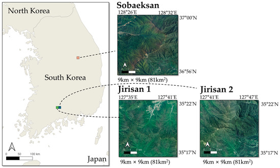
Figure 1.
Location of the study areas. The map on the left shows the locations of Sobaeksan National Park (orange) and Jirisan National Park (green) within South Korea. The panels on the right display satellite images of the 9 km × 9 km regions: Sobaeksan, Jirisan 1, and Jirisan 2.
Since the reference label data used in this study was based on the year 2022, satellite data from 2022 were utilized, incorporating imagery from a total of 12 time points. Data was collected at approximately monthly intervals. To more precisely capture species-specific characteristic differences during the leaf-out and leaf senescence periods, additional data were acquired at 15-day intervals during specific periods. From 1 April to 1 June, data were collected every 15 days to better capture inter-species differences during leaf-out. Similarly, from 1 October to 1 November, data were additionally acquired in the same manner to accurately capture observable inter-species differences during leaf senescence. The data collection schedule is summarized as follows. However, if data for a specific date could not be obtained due to weather conditions or other factors, the closest available date’s data was used instead. Table 1 details the selected target dates and the actual data acquisition dates for each satellite and site.

Table 1.
Summary of dates from obtained data.
Satellite Imagery
This study utilized Sentinel-2 and PlanetScope satellite data. Sentinel-2, operated under the Copernicus program, is a multispectral satellite providing a total of 13 spectral bands. We used Sentinel-2 Level-2A products, incorporating data from both the Sentinel-2A and Sentinel-2B satellites. Sentinel-2 offers the advantage of providing a variety of spectral bands, particularly including those critical for tree species classification, such as red edge, near-infrared (NIR), and shortwave infrared (SWIR) bands, making it highly suitable for this research. The significance of these bands in satellite image-based tree species classification tasks has been demonstrated in numerous previous studies.
In addition, PlanetScope [31] satellite data, which employs over 150 microsatellites (Dove series), was utilized to provide high-resolution imagery with an average revisit period of less than one day. This study employed PlanetScope imagery labeled as PSScene, captured via the SuperDove constellation. These data consist of orthorectified images with a ground sampling distance of 4.1 m and a spatial resolution of 3 m per pixel. The SuperDove satellites, launched based on the latest Dove-R platform beginning in 2020, offer an enhanced eight-band multispectral configuration and improved radiometric calibration compared to previous Dove-Classic and early Dove-R satellites.
The data used in this study were obtained through Planet’s Education & Research Program, which restricted access to four of the eight available bands: red, green, blue, and NIR. Given the study’s objective of analyzing the precise spatial distribution of tree species, satellite imagery with higher spatial resolution than Sentinel-2 was required, and PlanetScope imagery met these criteria. Notably, the program permitted free access to data within a monthly limit of 3000 km2, allowing its utilization in alignment with the research objectives. The specific satellite bands and spatial resolutions used in this study are summarized in Table 2. Among these, Sentinel-2 bands B02, B03, B04, and B08 were used exclusively for the spectral reflectance processing. The final input dataset for the tree species classification model consisted of PlanetScope’s blue, green, red, and NIR bands, along with Sentinel-2’s B05, B06, B07, B8A, B11, and B12 bands.
Table 2.
The summary of used imagery.
3. Methodology
3.1. Super Resolution
As previously mentioned, Sentinel-2 data includes diverse bands; however, its spatial resolution is coarse for tree species classification. Since this study aimed to generate a high-resolution tree species map, a dataset of higher spatial resolution was necessary. Furthermore, we intended to verify the necessity of forest texture characteristics. However, we assumed that PlanetScope’s spatial resolution was at least 6 to 8 times greater than that of Sentinel-2, which could impede model learning. Therefore, our approach, depicted in Figure 2, involves applying an SR technique to the Sentinel-2 data to enhance its resolution before classification
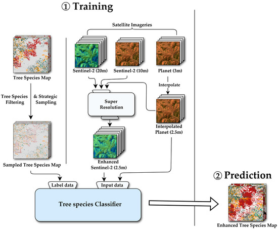
Figure 2.
Overall methodological workflow. Schematic overview of the processing pipeline, from data acquisition for Sentinel-2 and planet imagery and preprocessing to model training and prediction to generate the enhanced tree species maps.
Following Wald’s protocol, we applied an SR methodology for Sentinel-2 images based on planet images in this study, which closely resembles the methodology described in [32]. In contrast to traditional SR problems, this method can leverage the ability to use medium-resolution Sentinel-2 bands fused with PlanetScope imagery to achieve better SR results. The following are the precise methods used in this research:
- First, PlanetScope data, which has a 3 m spatial resolution, is resampled to 2.5 m resolution using bicubic interpolation. This step is performed to ensure that the native resolutions of Sentinel-2 imagery (e.g., 10 m, 20 m) are integer multiples of the target as PlanetScope resolution.
- Subsequently, all images are downsampled by a factor of 1/8 using the nearest neighbor method to generate the training dataset. As a result, Sentinel-2 bands are downsampled to resolutions of 160 m from the previous 20 m bands and 80 m from the previous 10 m bands, while the PlanetScope imagery is downsampled to a 20 m resolution. These downsampled images serve as the input data for training the SR model. The original, non-downsampled Sentinel-2 images which have spatial resolution of 10 m and 20 m, are used as the ground-truth data.
- Next, training data is trained to be performed SR using a residual convolutional neural network (RCNN). The Sentinel-2 bands, which have been downsampled to 160 and 80 m, are first upsampled to a common 20 m resolution using subpixel synthesis [33], by upsampling factors of ×8 and ×4, respectively. These upsampled Sentinel-2 bands are then concatenated band-wise with the 20 m PlanetScope imagery. The resulting multi-band tensor is passed through a series of residual convolution blocks to produce the output. The model is trained to minimize the L1 loss between this output and the ground truth, which is the concatenation of the original Sentinel-2 images at 20 m and 10 m resolution. In this study, RCNN used 10 residual convolution blocks to train a model with approximately 154K parameters. The model was trained for a total of 100 epochs.
- The trained SR model is applied to the original 10 m and 20 m Sentinel-2 images, as well as the 2.5 m PlanetScope image without downsampling. For all processed Sentinel-2 bands, this process produces images with a resolution of 2.5 m. The subsequent species classification work of this study used the 2.5 m super-resolution Sentinel-2 band and 2.5 m PlanetScope imagery as input data. Figure 3 shows an example of SR results.
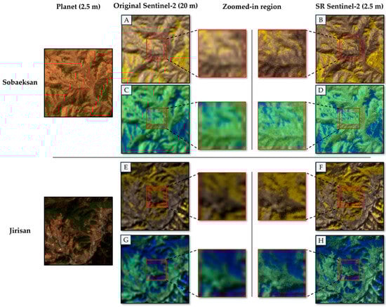 Figure 3. Examples of SR Sentinel-2 imagery in the Jirisan and Sobaeksan areas. (A,B,E,F) are false-color composites of B05, B06, and B07, while (C,D,G,H) are composite of B8A, B11, and B12. The zoomed-in region is an enlarged portion of the 20 m Sentinel-2 image, which is super-resolved at 2.5 m. The spatial resolution of SR Sentinel-2 was generated via 8× SR.
3.2. Label Data
In this study, labels for training were generated using tree species map data provided by the Korea Forest Service (https://map.forest.go.kr, accessed on 18 December 2024). The 1:5000-scale forest-type map, used for these labels, was produced through a multi-stage process. Initially, basic data such as aerial photographs, project status maps, forest management records, and existing 1:25,000-scale forest-type maps were collected and analyzed. This was followed by on-site verification and correction of stand delineations and attributes derived from an interpretation of aerial imagery, complemented by surveys of circular sample plots (11.28 m radius) at the center of each map sheet. It is important to note that the foundational 1:25,000 scale forest-type map, one of the base materials, was developed in part from the National Forest Resource Inventory, which was conducted in five phases, with the first phase spanning a wide period from 1972 to 2010. Using these preceding data, the 1:5000 scale forest-type map underwent its second update in 2022.
However, this 1:5000 map is subject to certain limitations. Due to the broad temporal scope of the source 1:25,000 map, it may not always accurately reflect the current tree species distribution within stands. Furthermore, even though the 1:5000 map was produced by incorporating some field surveys and aerial photo interpretation, discrepancies can exist with actual on-the-ground forest conditions, which change dynamically due to natural processes such as disturbances like wildfires. Additionally, because it is impractical to survey every individual tree within a 5 km2 area, the mapping process relies on central sampling. This inherent sampling approach means there is a possibility that the map may not fully reflect the actual dominant tree species or the precise species composition for every specific location within that 5 km2 area. These limitations suggest potential inaccuracies in the map data.
A total of five major tree species were selected: PD, PK, and LK, the most common coniferous species in Korea, and QM and QV, representative broadleaf species. With the addition of a non-forest (NF) class, the final dataset included six classes. Pixels classified as these specific classes in the tree species map were selected and used as training data. The tree species map includes a significant number of areas that are not assigned to a single species, such as coniferous forests, broadleaf forests, and mixed coniferous-broadleaf forests. In this study, these mixed-species areas were excluded, and only pixels classified as a single species were utilized for training.
Table 3 presents the distribution of pixels for each tree species class per region, with the original counts and proportions before sampling shown on the left side, and the post-sampling distribution presented on the right. As shown on the left side of Table 3, directly using the initial data for training may degrade performance for minority classes due to severe class imbalance. Moreover, if certain species are concentrated in specific regions, the model may be overfit to region-specific patterns, resulting in poor classification performance for species distributed across minority areas. Additionally, using the entire dataset would substantially increase the computational resources required for training. To address these challenges, we introduced a sampling strategy that limits the number of samples per class within each region. Specifically, if the number of pixels for a particular species class exceeded 15,000 within a region, 15,000 samples were uniformly selected; otherwise, the entire data for that class were used. This approach is fundamentally based on Random Under-Sampling (RUS) in [30]. RUS is a data-level sampling method that balances the number of samples per class by selectively discarding samples from the majority class. A key benefit of the RUS method is its ability to reduce bias towards the minority class (e.g., PK class). Additionally, it allows for the effective utilization of restricted computational resources by reducing the overall training dataset size. Furthermore, to mitigate sample concentration within specific spatial areas of a region, samples were evenly extracted by sequentially iterating through spatially distinct units (box numbers; see Section 3.3). This method prevents training biases toward specific areas and ensures a balanced inclusion of data from diverse spatial locations, thereby preserving information diversity.
Table 3.
The number of original and sampled pixels by each species code and region.
Figure 4 illustrates an example of the sampling process for the QM class in the Jirisan 1 region. As shown, sample pixels were extracted evenly across the entire region. The final number and proportion of samples per class in the constructed dataset are summarized on the right side of Table 3. After sampling, the smallest class, PK, accounts for 12.0% of the total samples, while the largest class, QM, accounts for 19.6%, indicating a substantial reduction in class imbalance compared to the original distribution. The regional distribution bias was also significantly improved.
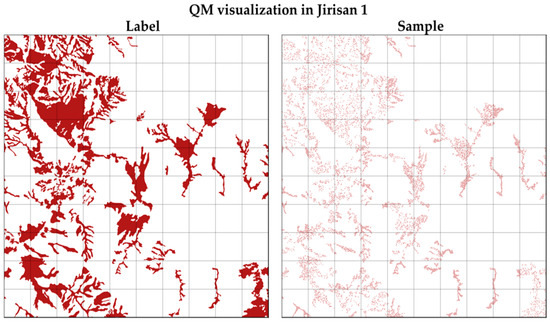
Figure 4.
The visualization of strategic sampling applied on Jirisan. It visualizes the QM distribution on the left side and the spatially uniformly extracted training samples on the right side.
3.3. Selected Models Using Single-Pixel Classification
To explore the most effective model architecture for this approach, various candidate models were designed, including a linear model, RF, a multi-layer perceptron (MLP) [34], SEB-linear using a spectral encoder block (SEB), and a SEB-transformer using SEB and a transformer [35]. The linear model was employed as a baseline, flattening the (time, bands) input into a one-dimensional vector and mapping it directly to class predictions through a single linear layer. This approach is conceptually related to the linear transformation that underlies linear discriminant analysis (LDA) [36]. However, in our implementation, the parameters of the linear layer were optimized through standard neural network training procedures, rather than using Fisher’s criterion for maximizing class separability. Band-wise normalization was applied beforehand to emphasize relative changes in band values across time steps, enhancing feature learning despite the model’s limited capacity. The linear model consisted of only 726 parameters, representing a minimal structure. All models were trained for 100 epochs using the AdamW optimizer [37] and a scheduler using learning rate by cosine annealing [38]. AdamW, a variant of the Adam optimizer, separately applies weight decay to better reflect L2 regularization. A learning rate and weight decay of 5 × 10⁻⁴ were used, identified as optimal in preliminary tests. The scheduler gradually reduced the learning rate over the entire 100 epochs, promoting both rapid early convergence and stable training. This configuration was consistently applied to all subsequent DL models.
RF has consistently demonstrated stable performance across various classification tasks and is widely used for its lightweight structure, interpretability, and efficiency. In the field of tree species classification, RF has often been utilized as a fundamental baseline model. Accordingly, RF was adopted in this study as a representative traditional ML learning technique. All hyperparameters for the RF classifier were kept at their default settings. Compared to the linear classifier, RF can capture more complex non-linear relationships, achieving relatively high performance even with a simple structure. Thus, RF was employed to evaluate the performance limits of traditional ML methods and, through comparison with subsequently introduced DL-based models, to assess whether DL can substantially contribute to improving single-pixel tree species classification.
MLP was introduced to evaluate performance when the model learns without explicit inductive biases, relying solely on a sufficient number of parameters. The MLP follows a typical deep neural network structure, where each block consists of a linear layer, batch normalization [39], a sigmoid linear unit (SiLU) activation function [40], and dropout [41]. This block is repeated three times, resulting in approximately 98,000 parameters. The input data, flattened into a 1D vector, passes through multiple hidden layers to learn complex non-linear relationships. This model contrasts with the SEB-linear and SEB-transformer architecture, which explicitly incorporate inductive biases to separately model spectral and temporal dimensions. Comparing these models provides insights into the effectiveness of different modeling strategies.
Both the SEB-linear and SEB-transformer share a spectral encoder module to extract features from the spectral dimension. The spectral encoder first projects the input into a higher-dimensional feature space using a linear layer, applies batch normalization for distribution stabilization and employs the SiLU activation for non-linear transformation. By repeatedly applying a second linear layer, batch normalization, and SiLU, the encoder progressively compresses the features into an embedding dimension. Finally, dropout is applied to mitigate overfitting and enhance generalization. Configured this way, the spectral encoder effectively captures meaningful spectral features from the input data.
The SEB-linear is based on the spectral encoder and adopts the simplest structure for learning temporal information. Spectral information for each time point is extracted using the spectral encoder, forming a sequence of shapes (times, embedding dimension). This sequence is then flattened into a single vector, and a linear layer is applied for final classification. The model contains approximately 31,000 parameters and is designed to process temporal information with minimal structural complexity. It serves as a baseline for comparing performance with more sophisticated temporal modeling architectures.
In contrast, the SEB-transformer is designed to learn temporal patterns more effectively by adding a transformer encoder after the spectral encoder. The sequence output from the spectral encoder is input into the transformer encoder, which captures time-series patterns through a self-attention mechanism. The resulting output is flattened, and a linear head performs the final classification. With a total of approximately 98,000 parameters, this model is capable of processing temporal information more intricately than SEB-linear. The transformer-based model aims to assess the extent to which a high-capacity architecture improves performance compared to a simple linear approach for temporal information processing. The detailed structures of the MLP, SEB-linear, and SEB-transformer are illustrated in Figure 5.
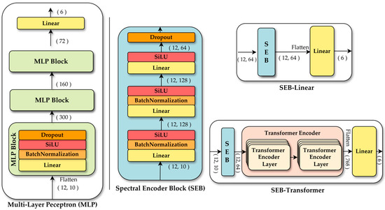
Figure 5.
Architecture of the DL models used for single pixel-based tree species classification: MLP and two models using spectral encoder block (SEB): SEB-linear and SEB-transformer.
3.4. Evaluation Metrics
To effectively separate the training, validation, and test datasets, each study region was divided into 100 grid cells (boxes). Through this process, the three study regions were each subdivided into 100 smaller boxes, facilitating the construction of spatially separated datasets and enabling a more accurate assessment of the model’s generalization performance. From each region, two boxes exhibiting minimal class imbalance and sufficient representation of the target tree species were selected for the test set. The remaining boxes, excluding those allocated for testing, were divided into five mutually exclusive groups for 5-fold cross-validation. This systematic, grid-based approach to data splitting, ensuring spatial separation between training and validation sets across folds, aligns with the principles of robust spatial cross-validation highlighted by [42] for remote sensing applications. Such strategies are crucial for obtaining reliable estimates of model performance when dealing with spatially autocorrelated data. The specific structure of the data split is illustrated in Figure 6.
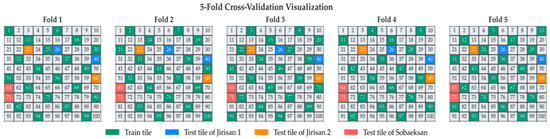
Figure 6.
Visualization of the 5-fold cross-validation data split. The study area is divided into 100 tiles, showing the allocation of training tiles (green) and region-specific test tiles (Jirisan 1: blue; Jirisan 2: orange; Sobaeksan: red) for each fold.
During model development, quantitative evaluation metrics were used to evaluate agreement with ground-truth data. To analyze model performance in greater detail and to enhance intuitive understanding, four specific classification tasks were defined for evaluation:
- NF vs. forest: a binary classification task distinguishing NF area from forest areas across the entire study area.
- Conifer vs. broadleaf: a binary classification task distinguishing conifer from broadleaf within areas correctly classified as forest.
- Intra-conifer classification: classification among three coniferous species—PD, PK, and LK—within areas correctly classified as conifer.
- Intra-broadleaf classification: classification between QM and QV within areas classified as broadleaf.
For each of these four classification tasks, evaluation metrics such as accuracy, macro-averaged precision, and macro-averaged recall were calculated and utilized. For precision and recall, macro-averaging was applied instead of weighted averaging to ensure equitable evaluation across classes. This approach was adopted because, although the sampling process mitigated class imbalance to some extent, differences in the number of instances between classes still remained, and macro-averaging minimizes the impact of such subtle imbalances on model performance evaluation.
To compare model performance, 5-fold cross-validation was performed for each model. The final performance evaluation was based on the prediction results from the epoch that exhibited the best validation performance in each fold. For all folds, macro-averaged precision and macro-averaged recall were measured for each of the four defined classification tasks (NF vs. forest, conifer vs. broadleaf, intra-conifer classification, intra-broadleaf classification). This yielded a total of eight performance metrics per fold for each model. Consequently, through 5-fold cross-validation, a total of 40 quantitative performance metrics (5 folds × 4 tasks × 2 metrics) were obtained per model.
To assess the statistical significance of the collected performance metrics, the Friedman test was conducted. To analyze performance differences between models in more detail, a post hoc Nemenyi test was additionally performed. The Friedman test is a non-parametric method used to determine whether the performance differences among multiple models evaluated on the same dataset are statistically significant. If the Friedman test indicated a significant difference in the average ranks of the models, additional multiple comparison analysis was required. Accordingly, the Nemenyi test was applied as a post hoc procedure to perform pairwise comparisons between models. The Nemenyi test compares the average rank differences among models to identify whether one model performs significantly better than others. In this study, the Nemenyi test was employed to analyze statistically significant differences in performance, based on which the optimal model was selected.
3.5. Experimental Design for Dimensional Importance Comparison
This study analyzed the importance of spectral, temporal, and spatial dimensions on model performance in the tree species classification task. To achieve this, we first defined the meaning of the information contained within each dimension and then designed experiments to analyze the influence of each dimension in isolation.
Spectral information refers to information obtainable through the relationships between different bands, encompassing characteristics like color, brightness, and saturation in both visible and non-visible light spectra. This spectral information reflects the physiological state or compositional differences of various vegetation types and has been considered a core element in previous remote sensing-based classification studies.
Spatial information relates to information derived from relationships with neighboring pixels. However, at the 2.5 m resolution used currently, capturing fine texture information originating from leaves or branches within individual trees is limited. Therefore, this study focused on analyzing whether the forest texture, formed by the arrangement of individual trees, is significant for tree species classification.
Temporal information encompasses information identified through relationships between 12 time points (Table 1), including interactions between spectral and spatial dimensions changing along the time axis. This information, reflecting vegetation growth cycles or seasonal changes, can play a crucial role in tree species classification using multi-temporal data.
Based on these definitions and the established importance of spectral information, we designed our experimental setup. Since spectral information has been widely recognized as key for tree species classification in previous research, the condition of removing spectral information was excluded from our experiments. Thus, this study focused on the following three experimental conditions: (Case 1) using only spectral information, (Case 2) using integrated spectral and spatial information, and (Case 3) using integrated spectral and temporal information.
4. Results
4.1. Comparative Evaluation of Classification Models
Table 4 shows the averaged task-specific accuracy, overall F1 score, and overall accuracy by model used. The averaged task-specific accuracy was derived from average accuracy via every trained model through each task, and the overall accuracy was calculated as an average of accuracy by each model after 5-fold cross-validation. The simple linear model achieved high accuracy in higher-level classification tasks, recording 98.41% for NF vs. forest and 94.15% for conifer vs. broadleaf. This indicates that combining spectral and temporal information from satellite imagery can be highly effective even with basic linear separation for classification tasks with relatively clear distinguishing features, such as forest/NF and conifer/broadleaf discrimination. Thus, when interpretability is a critical requirement, the linear model could be a viable choice for higher-level classification tasks.
Table 4.
Comparison of the performance of applied models. The highest performance values among the applied models are indicated in bold.
However, the linear model showed a marked decline in performance for finer-grained classification tasks such as intra-conifer and intra-broadleaf classification. Its accuracy for these tasks dropped to 87.51% and 71.93%, respectively, substantially lower than those of the other models discussed subsequently. This suggests that fine-grained classification tasks involve subtle and complex inter-class distinctions, necessitating greater model capacity and expressive power. In short, the limited capability of the linear model was insufficient for adequately learning these complex patterns. This necessitates the use of models with non-linear capabilities.
The RF model demonstrated overall improvements compared to the linear model. Notably, accuracy for the challenging intra-broadleaf classification improved by approximately 5.17 percentage points, from 71.93% to 77.10%. The overall F1-score and OA also increased to 80.02% and 81.36%, respectively. This improvement suggests that RF, as an ensemble method, can capture certain non-linear features and interactions through its combination of decision trees. Nevertheless, limitations in fine-grained classification performance remained.
The SEB-linear and SEB-transformer models, utilizing the spectral encoder, achieved further improvements over RF. Improvements were particularly noticeable in detailed species classification, with accuracies of 89.97% and 79.31% (SEB-linear) and 90.47% and 81.60% (SEB-transformer) for intra-conifer and intra-broadleaf classification, respectively. These results validate the effectiveness of the DL-based approach for learning spectral and temporal information in tree species classification tasks. Furthermore, the SEB-transformer consistently outperformed the SEB-linear across all tasks, highlighting the importance of effectively learning temporal information with a sufficiently expressive module following spectral encoding.
The MLP model exhibited the best overall performance in this evaluation. It recorded the highest accuracy for NF vs. forest (98.94%), conifer vs. broadleaf (95.75%), and intra-conifer (91.01%) classification tasks. Even for the most challenging intra-broadleaf classification, its accuracy of 81.43% was nearly tied with the SEB-transformer for the top performance. Consequently, MLP surpassed all other models in both overall F1-score (84.36%) and OA (85.38%), achieving the best comprehensive performance. Notably, it even slightly outperformed the SEB-transformer, which has a very similar number of parameters. This result suggests that allowing the model to directly learn useful patterns for tree species classification from the training data, rather than embedding specific inductive biases, may have been more suitable for the dataset and objective of this study.
DL-based models generally exhibited superior classification performance compared to traditional ML models, with the MLP model consistently demonstrating the highest performance. To assess the statistical significance of these performance differences, the Friedman test was conducted [43]. The results rejected the null hypothesis of no difference among the models at a confidence level of 0.05 (p < 0.001), confirming that the performance differences were statistically significant. Accordingly, for a detailed analysis of performance rankings and significant differences between models, we performed a post hoc Nemenyi test, which is a follow-up test to the Friedman test used for comparing the performance of multiple classifiers. When the Friedman test indicates a statistically significant difference, the Nemenyi test is used to identify specifically which pairs of classifiers reflect a significant difference.
The CD plot in Figure 7 depicts the Nemenyi test results. The position of each classifier on the graph represents its average rank, which is the sum of all evaluation metrics, precision and recall, for each of the four tasks. These metrics are calculated for each of the five cross-validation folds, with the model ranks averaged to produce a total of 40 individual metric values.
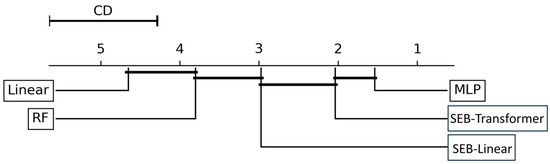
Figure 7.
Nemenyi post hoc test results (α = 0.05) comparing the performance of five classification models. Each classifier’s position on the graph reflects its average rank, computed by averaging its rankings across 40 evaluation metrics (precision and recall for each of four classification tasks, calculated over five cross-validation folds). The critical distance (CD) represents the threshold for statistical significance. Models connected by a horizontal bar do not exhibit statistically significant differences in performance.
A statistically significant performance difference exists between two models if the difference in their average ranks exceeds the CD. The analysis revealed that the MLP model achieved the best average rank. The connecting bars in the plot indicate groups of models whose average rank differences are within the CD, meaning no statistically significant performance difference exists between them. Specifically, the performance difference between the MLP and SEB-transformer was not statistically significant.
However, the Nemenyi test results clearly showed that the top-performing models, MLP and SEB-transformer, exhibited statistically significant performance differences compared to the SEB-linear, RF, and the linear model. The average ranks of MLP and SEB-transformer were significantly higher (exceeding the CD value) than those of the SEB-linear, RF, and the linear model. Furthermore, the SEB-linear also demonstrated statistically significantly better performance than both RF and the linear model. Although the Nemenyi test did not find a statistically significant difference between the MLP and SEB-transformer, the MLP model (1) recorded the highest values across most individual classification tasks and overall evaluation metrics, and (2) achieved the best average rank in the Nemenyi test. Therefore, based on the aggregation of this evidence, the MLP model was ultimately selected as the most suitable model for achieving the tree species classification goals of this study and was chosen for subsequent analysis and result generation.
4.2. Model Performance
Figure 8 presents the confusion matrix for the single fold that exhibited the best performance among the 5-fold cross-validation results for the finally selected MLP model. It showed that the MLP model performed well. In particular, the NF class achieved the highest individual accuracy at 96%, with 8943 samples correctly classified and very few misclassifications into other classes. Additionally, the LK class also showed high accuracy at 94%, recording a high true positive count of 9795. These results indicate the model’s strength in distinguishing NF areas and specific coniferous species.
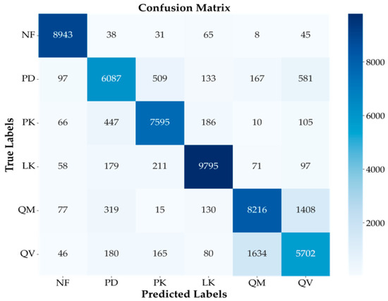
Figure 8.
Confusion matrix for the best-performing fold of the MLP model. Illustrates the classification performance across the six classes (NF, PD, PK, LK, QM, QV) and misclassification trends, particularly between similar species (PD/PK, QM/QV).
However, some confusion between classes was still observed. Notably, frequent mutual misclassifications occurred between PD and PK (509 cases of PD misclassified as PK and 447 cases of PK misclassified as PD). This suggests that the model struggled to distinguish between these two species belonging to the same Pinus genus, likely due to similarities in their spectral or temporal characteristics, reflecting the challenges of intra-conifer classification. In broadleaf classification, confusion between QM and QV was most prominent (1408 cases of QM misclassified as QV, and 1634 cases of QV misclassified as QM). This accounted for the largest proportion of all misclassification instances, clearly indicating that distinguishing between these two Quercus genus species was the most challenging task in this study. Both species share very similar spectral characteristics, ecological traits, and habitat preferences, making them inherently difficult to separate using satellite imagery. The possibility of hybridization in certain areas could further complicate clear distinction.
Despite these inherent similarities and classification challenges, the model achieved significant performance by correctly classifying a substantial number of samples for both QM (8216 true positives) and QV (5702 true positives). Nevertheless, for QV, the proportion of samples misclassified as QM (1634 cases) was relatively high compared to the number of correctly classified samples (5702 cases), suggesting that reducing misclassification for this class is a key focus for future model improvement. Additionally, some confusion was observed between other classes, such as PD being misclassified as QV (581 cases) and QM being misclassified as PD (319 cases). Overall, the confusion matrix analysis in Figure 8 confirms that, while the MLP model achieved high overall classification performance, challenges remain, particularly in distinguishing fine-grained species with similar characteristics within the same genus, such as PD/PK within Pinus and QM/QV within Quercus.
4.3. Enhanced Tree Species Map
Figure 9 and Figure 10 present examples where the original tree species map was enhanced using the prediction results from the model developed in this study. The target areas addressed in both figures include the following: (1) areas classified as one of the five main target species in the original tree species map, (2) NF areas, and (3) areas indicated with hatching in the figures. These hatched areas correspond to mixed forest regions in the original map where the species composition was too complex to allow classification into a specific single species and were thus broadly categorized as ‘broadleaf forest’, ‘coniferous forest’, or ‘mixed coniferous-broadleaf forest’. One of the key contributions of the model developed in this study is the generation of fine-grained tree species prediction information at the pixel level precisely in these hatched areas, where the original tree species map lacked detail, thereby significantly enhancing the information quality of the map.
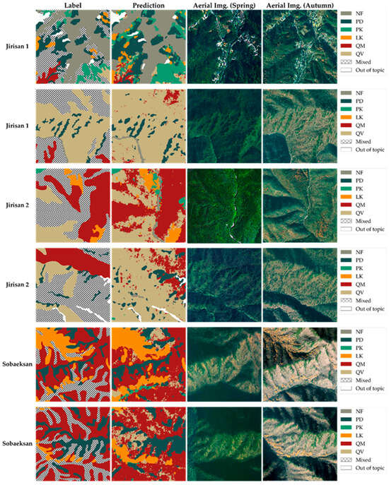
Figure 9.
Comparison of the original tree species map (label) and model prediction (prediction) in test areas (unseen data), with aerial imagery for reference. Demonstrates the model providing detailed information within the original mixed forest (hatched) areas.
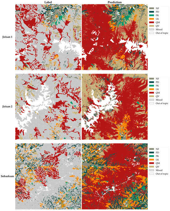
Figure 10.
Enhanced tree species map. Comparison between the original tree species map on the label side and the final, enhanced 2.5 m resolution model-predicted tree species map on the prediction side for the entire study areas.
Figure 9 validates this improvement by showing the model’s prediction results for an independently separated test area. All pixels in this area consist of unseen data not used for model training, enabling a visual evaluation of the model’s generalization performance and species prediction accuracy under real-world conditions. As shown in the figure, the model’s predictions for areas classified as single species in the original map exhibit high agreement with the ground truth labels. Moreover, the model successfully generated detailed predictions within the hatched areas, overcoming the limitations of the original map and improving the overall information detail. Comparisons with ultra-high-resolution (0.25 m) aerial orthorectified images from the National Geographic Information Institute in South Korea allow visual verification that the model’s predictions reasonably reflect the actual vegetation distribution in Figure 9 and Figure 11.
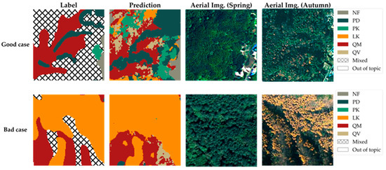
Figure 11.
Test area prediction results, which are comparisons of good cases (detailing mixed forests) and bad cases (LK boundaries).
Figure 10 presents the final enhanced tree species map, generated by applying the model’s predictions across the entire study area. Based on the performance demonstrated in the test area shown in Figure 9, this map represents the final output, where the quality and detail of the tree species map have been improved across the entire study site. Through the enhanced tree species map in Figure 10, it is now possible to ascertain the specific distribution of tree species within previously broadly categorized hatched areas, enabling a more precise and fine-grained understanding of vegetation distribution throughout the study area.
5. Discussion
5.1. Detailed Analysis of the Enhanced Tree Species Map
Figure 11 presents magnified views of selected notable areas from the test areas shown in Figure 9, facilitating a detailed analysis of the prediction results from the model proposed in this study. It encompasses both instances where the model’s predictions were successful as a good case and instances where the prediction accuracy warrants further examination as a bad case.
First, the area presented as the good case serves as a representative example where the model provides significantly more detailed information compared to the original tree species map. As previously mentioned, the hatched areas on the original tree species map, which could not be classified under a single species, likely represent areas where identifying a specific dominant species was challenging or where multiple species coexist in a mixed forest setting. Indeed, the model predicts these areas as complex mosaics comprising various classes, including QM, QV, PD, PK, LF, and NF. This reveals the specific vegetation composition within the mixed forest, information unattainable from the original map. Naturally, the possibility that these areas represent communities of other species not included in the model’s training data cannot be entirely ruled out. However, considering that the six main classes classified by the model (QM, QV, PD, PK, LF, and NF) constitute most of the forest cover below 1000 m elevation within the Jirisan 1 region, it is highly probable that these hatched areas are indeed mixed forests composed of these dominant species. A visual inspection of aerial imagery—especially the autumn image with its distinct color variations—supports this prediction by revealing a heterogeneous canopy with a mix of colors and textures, consistent with the complex mixed forest composition predicted by our model. Therefore, the model demonstrates its potential to contribute to a more precise understanding of forest resources by effectively generating high-resolution information on the detailed species distribution within mixed forests—details unavailable in the original map.
Conversely, the area presented as the bad case exemplifies instances where the model’s predictions appear less accurate in reflecting the actual forest conditions compared to the original tree species map. When compared with the aerial photograph of the corresponding area, the boundary of the LK community delineated on the original map appears to align more closely with the actual vegetation boundary. The model’s prediction exhibits a tendency to classify certain areas as LK, even where the aerial photograph suggests otherwise. This discrepancy is likely attributable primarily to the spatial resolution limitations of the satellite imagery used as input for the model. While the satellite imagery used in this study was significantly enhanced to 2.5 m resolution through SR, it still possesses considerably lower resolution compared to ultra-high-resolution aerial imagery (e.g., 0.25 m). Traditional methods for creating forest maps involve skilled personnel manually interpreting such ultra-high-resolution aerial photographs to delineate boundaries. Consequently, to delineate the boundaries of relatively distinct, single-species stands like the LK community shown, the original map might occasionally offer greater accuracy than the model’s output.
Nonetheless, as clearly demonstrated in the ‘good case’ of this study, the high-resolution tree species maps generated by our model exhibit distinct improvements in terms of detail and objectivity compared to the original reference tree species map used as the basis for training. This enhancement is possible because the original map was treated as a ‘weak label,’ and its inherent limitations were addressed. Notably, the original map is provided at a spatial resolution of 30 m, which imposes significant limitations in accurately representing tree species distribution.
Our model addresses these limitations. Firstly, the enhanced tree species map can provide detailed 2.5 m pixel-level information on tree species distribution in complex mixed forest areas, which was often not sufficiently represented in the original map. This means that generalized ‘mixed forest’ labels from the original map can be disaggregated into a mosaic of individual species. Secondly, the artificial intelligence model systematically learns and utilizes subtle spectral–temporal patterns from satellite imagery across both visible and non-visible wavelengths. This allows it to capture minute vegetation differences that are difficult for the human eye to discern thereby increasing classification accuracy. In other words, while learning from the initial labels provided by humans (the original tree species map), the model is trained to extract the most consistent and recurring spectral–temporal patterns from the data. This process allows it to filter out potential noise or individual inconsistencies in the labels.
Therefore, despite the potential for some inaccuracies in specific boundary delineations due to the limitations of satellite image resolution (as seen in the ‘bad case’ for LK boundaries), the high-resolution tree species maps generated via this model will serve as valuable and effective resources, providing the more detailed and objective information necessary for understanding and managing complex forest structures, compared to the original reference data. By synergistically utilizing the original tree species map data and the high-resolution maps generated via this model, it is anticipated that both accurate boundary delineation for single-species stands and detailed internal composition information for mixed forests can be effectively obtained, thereby elevating the quality of forest resource information.
5.2. Dimensional Importance Comparison
This study aimed to quantitatively analyze the respective impacts of spectral, temporal, and spatial dimensions on model performance in the tree species classification task. Table 5 presents experimental results. First, it was noteworthy that over 80% overall accuracy (OA) could be achieved using only spectral dimension information. This strongly suggests that spectral information plays a critical role in tree species classification. Indeed, observations of forests from aerial photographs reveal clear color differences among tree species; for instance, conifers generally appear dark green, while broadleaf trees tend to exhibit lighter colors. These differences become even more pronounced during leaf-out and senescence periods. Utilizing invisible bands beyond the visible spectrum is likely to provide additional useful information for species classification.
Table 5.
Comparison of dimensional importance.
Second, spatial dimension information did not appear to significantly contribute to model performance improvement. In most tests, the performance of Case 2 (with spatial information) was lower than that of Case 1 (spectral information only). This indicates that spatial information acted as a hindrance to tree species classification. It suggests that, for the dataset and classes used in this study, differences in forest texture did not provide meaningful assistance for classification. The results obtained in this study support the effectiveness of the pixel-based classification framework, not only within the context of our own analysis but also in line with previous studies that adopted similar methodologies [18,19,20]. Furthermore, we determined that a patch-based input could introduce ambiguity in our specific research context. Our study relies on a coarser-resolution reference map for ‘weak labels,’ where spatially adjacent pixels often share the same label, even though the actual ground area may contain a mix of species. In such a scenario, training a model with patch-level inputs could compel it to predict the dominant species within the patch rather than the precise characteristics of the central 2.5 m pixel. This would effectively become a different task—classifying the dominant species of a patch—and could hinder the goal of generating a truly high-resolution, pixel-level map. Therefore, considering this experimental evidence and the potential for ambiguity, we opted for a pixel-based input method despite the many successful examples of patch-based CNNs in prior tree species classification research.
Third, temporal dimension information was found to significantly enhance the model’s classification performance. This implies that considering temporal changes, in addition to spectral information obtained at individual time points, plays an important role in tree species classification. The performance improvement was particularly notable in relatively difficult tasks, such as intra-broadleaf and intra-conifer classification. This confirmed that, for fine-grained classification within the same category, spectral information from a single time point alone is insufficient and that incorporating temporal information is essential. It can be concluded that when designing a tree species classification model, ensuring robust learning of spectral dimension information and actively leveraging temporal information is more effective than incorporating spatial information. These findings provide experimental justification for the multi-spectral, multi-temporal, single-pixel input approach adopted in this study’s model design.
5.3. Considerations for Applicability and Generalization of the Study
The methodology proposed in this study presents two primary application scenarios. The first is the SR enhancement of existing medium-resolution tree species maps. This is a core focus of our research, proposing a method to refine the quality of tree species maps in regions where such data already exist. Specifically, data points from the target area for enhancement are strategically sampled, and existing medium-resolution tree species maps are utilized as ‘weak labels’ to train a pixel-level dominant tree species classification model. By applying the trained model to the same region, an improved spatial resolution can be achieved compared to the original maps, and information gaps, particularly in challenging areas like mixed forests, can be effectively supplemented. This approach is potentially applicable to any region with existing medium-resolution tree species maps, provided they offer sufficient thematic detail to serve as effective ‘weak labels’. Considering that many countries worldwide establish and manage their own forest inventories, our methodology demonstrates high scalability.
The second application scenario is a more challenging task: applying an already trained model to geographically new, unseen regions. This method could enable the initial generation of tree species maps for areas where they are not yet available or are difficult to access. Successful implementation of this approach requires that a model trained on a specific source domain and time-period can effectively generalize new target domains and data acquisition times. This can be achieved by ensuring the model’s generalization performance through learning universal features, or by utilizing training data that shares similar ecological and phenological characteristics with the target application area. Ultimately, a complementary combination of these two strategies is expected to effectively enhance prediction accuracy in new regions.
5.4. Novelty of This Study
This study proposes an integrated framework that enhances existing national tree species maps by treating them as weak labels and applying SR techniques to multi-temporal satellite imagery, ultimately generating high-resolution (2.5 m) tree species maps. Compared to previous research, the proposed approach offers several key contributions.
First, it provides a practical solution to the challenges of label data acquisition and scalability. While prior studies have acknowledged the inherent inaccuracies in national tree species maps, their attempts to correct or re-label the maps have required substantial time and resources, limiting their applicability to broad areas. In contrast, this study treats maps as weak labels, proposes strategies to manage label noise, and validates their effectiveness, establishing a scalable framework that does not require additional labeling efforts. This pragmatic approach reflects the perspective that, in DL model training, the quantity and diversity of data can sometimes be more critical than perfect label accuracy.
Second, it effectively overcomes the spatial resolution limitations of Sentinel-2 imagery. Previous studies [15,19] were constrained by Sentinel-2’s 10 m resolution, while [13] combined Sentinel-2 with RapidEye (5 m) using basic nearest neighbor interpolation without advanced SR fusion. In contrast, this study applies an SR technique, using PlanetScope (3 m) imagery as a reference, to construct a 2.5 m high-resolution dataset. This dataset enabled pixel-level classification, allowing precise delineation of complex mixed forest boundaries and small-scale stands.
Third, the study successfully distinguishes between two major oak species, QM and QV, which are widespread in Korea and account for approximately 66% of the country’s oak forest area [44,45]. Despite their highly similar spectral and ecological characteristics, which have led previous studies to group them as a single class, this study leverages the expressive power of high-resolution multi-temporal datasets and DL models to classify them separately with over 81% accuracy (Figure 8). This demonstrates the effective learning of subtle spectral-temporal differences not previously captured and suggests the methodology’s broader applicability to classification challenges involving spectrally similar species.
5.5. Limitations and Future Works
Owing to the data access constraints of the Planet’s Education & Research Program, which limits monthly downloads, and available computing resources, this study was unable to construct a large-scale dataset. However, acquiring additional data from diverse time periods and geographical locations is essential to enhance the temporal and spatial generalization performance of the model. This is expected to facilitate the construction of models with more robust generalization capabilities. Furthermore, this study analyzed only five tree species due to the lack of sufficient training data for several minor species. With adequate data for additional major species such as Pinus rigida, Quercus acutissima, and Chamaecyparis obtusa, it would be possible to build a model capable of distinguishing a broader range of classes. Given that this study successfully classified QM and QV—species with very similar spectral and ecological characteristics—with over 81% accuracy, even more effective performance can be anticipated for species with greater differences.
One of the key advantages of constructing tree species maps using satellite imagery is the ease of updating them in response to dynamic changes. However, the model proposed in this study uses imagery from 12 time points as input, and there is a risk that its predictions could become ambiguous if changes occur at specific points in time. For instance, if an area originally classified as forest transitions to NF due to events such as logging, the model’s interpretation may be unclear. This potential vulnerability to intermediate changes was not considered in the current study. This issue can be addressed through two approaches.
The first is a data-driven approach: providing training data that includes examples of changes, thereby guiding the model to correctly predict the post-change class. However, a key limitation of this method is constructing large-scale time-series datasets for change detection. This is challenging because it requires obtaining sufficient cloud-free imagery that precisely captures events like logging, afforestation, and wildfire, which are themselves temporally infrequent and spatially variable. Therefore, this must be pursued in parallel with a model-driven approach. The model-driven approach involves defining a distance metric to quantify differences between satellite images over time. If significant changes are detected at a specific time point, the model could be designed to handle that time point separately, allowing it to reflect post-change information more accurately. By combining both data- and model-driven approaches, it is possible to develop a tree species classification model that is sensitive to dynamic forest changes. This is proposed as a future direction for research. Additionally, while this study concluded that forest texture information was not particularly useful at the current satellite image resolution, it is possible that texture information could play a more significant role if higher-resolution imagery were used. Future studies should investigate models that can effectively utilize forest texture information with ultra-high-resolution data.
This study utilized data from Sobaeksan and Jirisan National Parks, which are representative temperate forest regions in Korea. These regions are characterized, firstly, by four distinct seasons, leading to clearly distinguishable phenological patterns for different tree species, such as leaf-out, leaf-fall, and growing season [46]. Secondly, being mostly mountainous terrain, microclimates develop due to various topographic factors such as changes in elevation, slope, and aspect, leading to the formation of diverse microhabitats and vertical stratification. This environment results in complex vegetation distribution, high species diversity, and notably, the frequent occurrence of mixed forests [47]. Considering these characteristics of the study sites, the first application scenario—the enhancement of tree species maps within the same region—was deemed highly effective. The distinct seasonal changes maximized the advantages of using multi-temporal data by inducing clear differences in seasonal spectral signatures among species, while the presence of complex mixed forests and microhabitats strongly supported the necessity for high-resolution analysis via SR and a pixel-based approach. The high performance of the MLP model in this study, effectively learning these regional characteristics, can be understood in this context.
However, several considerations arise when extending the trained model to new regions, as in the second application scenario. A model trained with data from this study would likely face difficulties if directly applied to forests with markedly different ecological characteristics, such as subtropical evergreen broadleaf forests with less seasonal spectral variability, or boreal coniferous forests with relatively simple species composition. Even when applied to similar temperate forest regions, local differences in topography, soil, and microclimate can lead to diverse variations in phenological patterns or dominant species composition, making it difficult to expect that a model trained solely on Sobaeksan and Jirisan data has learned universally generalizable features. Furthermore, because these two study sites are national parks relatively shielded from human intervention, the model’s generalizability to forests outside of protected areas may be further limited. It is also uncertain whether the MLP model, which performed well in the first application scenario by effectively learning the characteristics of the study area, would maintain the same superiority in the second scenario. For successful generalization to other regions, models with explicit inductive biases regarding data structure, such as SEB-Linear or SEB-transformer, might offer better generalization by reducing overfitting. While the validation of such cross-regional application is beyond the scope of this study, it remains a crucial research task for enhancing the feasibility of the second application scenario in the future.
6. Conclusions
This study has proposed a novel methodology for generating high-resolution (2.5 m) tree species classification maps by applying DL-based models to multi-temporal, multi-spectral Sentinel-2 and PlanetScope satellite imagery. Notably, it introduced a method for creating more precise, high-resolution maps by effectively utilizing existing noisy, medium-resolution tree species map data as labeling data through appropriate sampling, even in the absence of high-resolution ground truth labels. This approach is of significant practical value, as it can be easily scaled to most regions in South Korea where tree species map data currently exist. The application of this methodology to Sobaeksan and Jirisan National Parks demonstrated its practical applicability, achieving over 85% overall accuracy (OA) and over 81% classification performance even for challenging species such as QM and QV. Additionally, the study provided experimental evidence supporting the model design decisions. It confirmed that spectral dimension information contributed most significantly to tree species classification performance and that the integration of temporal information further enhanced performance. In contrast, the incorporation of spatial information was found to hinder learning, supporting the effectiveness of a multi-spectral, multi-temporal, single-pixel-based model design. Furthermore, it was experimentally verified that a simple MLP structure outperformed models incorporating more complex inductive biases.
However, the study faced limitations due to constraints on PlanetScope data usage and available computational resources, resulting in insufficient spatio-temporal diversity and the analysis being limited to a small number of species. Future work involving the construction and training on extensive time-series data from diverse geographical areas is expected to enable the classification of a broader range of species and achieve superior generalization performance. In conclusion, this study presents a practical and scalable method for generating high-resolution tree species classification maps based on multi-spectral, multi-temporal satellite imagery using medium-resolution tree species maps. Its effectiveness was demonstrated through real-world applications, underscoring their academic and practical significance.
Author Contributions
Writing—original draft, T.C. and S.J.; writing—review and editing, B.K.; supervision, S.P. All authors have read and agreed to the published version of the manuscript.
Funding
This work was supported by the Seoul National University of Science and Technology.
Data Availability Statement
PlanetScope data can be downloaded from the PlanetScope Education and Research (E&R) Program (https://api.planet.com, accessed on 18 December 2024). The Sentinel-2 satellite data were provided as part of the European Union’s Copernicus Programme and are publicly available from the Copernicus Data Space Ecosystem (https://dataspace.copernicus.eu, accessed on 18 December 2024). The tree species map of The Republic of Korea can be downloaded from https://map.forest.go.kr (accessed on 18 December 2024).
Conflicts of Interest
The authors declare no conflicts of interest.
References
- Cavers, S.; Cottrell, J. The basis of resilience in forest tree species and its use in adaptive forest management in Britain. Int. J. For. Res. 2015, 88, 13–26. [Google Scholar] [CrossRef]
- Návar, J. Allometric equations for tree species and carbon stocks for forests of northwestern Mexico. For. Ecol. Manag. 2009, 257, 427–434. [Google Scholar] [CrossRef]
- Wang ChuanKuan, W.C. Biomass allometric equations for 10 co-occurring tree species in Chinese temperate forests. For. Ecol. Manag. 2006, 222, 9–16. [Google Scholar] [CrossRef]
- Mouret, F.; Morin, D.; Martin, H.; Planells, M.; Vincent-Barbaroux, C. Toward an operational monitoring of oak dieback with multispectral satellite time series: A case study in Centre-Val de Loire region of France. IEEE J. Sel. Top. Appl. Earth Obs. Remote Sens. 2023, 17, 643–659. [Google Scholar] [CrossRef]
- MacKenzie, W.H.; Mahony, C.R. An ecological approach to climate change-informed tree species selection for reforestation. For. Ecol. Manag. 2021, 481, 118705. [Google Scholar] [CrossRef]
- Taylor, D.; Kent, M.; Coker, P. Vegetation description and analysis: A practical approach. Geogr. J. 1993, 159, 237. [Google Scholar] [CrossRef]
- Crisco, W.A. Interpretation of Aerial Photographs; US Department of the Interior, Bureau of Land Management: Washington, DC, USA, 1983; Volume 287. [Google Scholar]
- Kim, K.; Lee, S. Distribution of Major Species in Korea (Based on 1:5000 Forest Type Map); National Institute of Forest Science: Seoul, Republic of Korea, 2013; p. 15. [Google Scholar]
- Fassnacht, F.E.; Latifi, H.; Stereńczak, K.; Modzelewska, A.; Lefsky, M.; Waser, L.T.; Straub, C.; Ghosh, A. Review of studies on tree species classification from remotely sensed data. Remote Sens. Environ. 2016, 186, 64–87. [Google Scholar] [CrossRef]
- Drusch, M.; Del Bello, U.; Carlier, S.; Colin, O.; Fernandez, V.; Gascon, F.; Hoersch, B.; Isola, C.; Laberinti, P.; Martimort, P. Sentinel-2: ESA’s optical high-resolution mission for GMES operational services. Remote Sens. Environ. 2012, 120, 25–36. [Google Scholar] [CrossRef]
- Breiman, L. Random forests. Mach. Learn. 2001, 45, 5–32. [Google Scholar] [CrossRef]
- Belgiu, M.; Drăguţ, L. Random forest in remote sensing: A review of applications and future directions. ISPRS J. Photogramm. Remote Sens. 2016, 114, 24–31. [Google Scholar] [CrossRef]
- Lim, J.; Kim, K.-M.; Jin, R. Tree species classification using hyperion and sentinel-2 data with machine learning in South Korea and China. ISPRS Int. J. Geo-Inf. 2019, 8, 150. [Google Scholar] [CrossRef]
- Maillard, P. Comparing texture analysis methods through classification. Photogramm. Eng. Remote Sens. 2003, 69, 357–367. [Google Scholar] [CrossRef]
- Lim, J.; Kim, K.-M.; Kim, E.-H.; Jin, R. Machine learning for tree species classification using sentinel-2 spectral information, crown texture, and environmental variables. Remote Sens. 2020, 12, 2049. [Google Scholar] [CrossRef]
- Cha, S.; Lim, J.; Kim, K.; Yim, J.; Lee, W.-K. Uncovering the Potential of Multi-Temporally Integrated Satellite Imagery for Accurate Tree Species Classification. Forests 2023, 14, 746. [Google Scholar] [CrossRef]
- Zhong, L.; Dai, Z.; Fang, P.; Cao, Y.; Wang, L. A review: Tree species classification based on remote sensing data and classic deep learning-based methods. Forests 2024, 15, 852. [Google Scholar] [CrossRef]
- Kowalski, K.; Senf, C.; Hostert, P.; Pflugmacher, D. Characterizing spring phenology of temperate broadleaf forests using Landsat and Sentinel-2 time series. Int. J. Appl. Earth Obs. Geoinf. 2020, 92, 102172. [Google Scholar] [CrossRef]
- Xi, Y.; Ren, C.; Tian, Q.; Ren, Y.; Dong, X.; Zhang, Z. Exploitation of time series sentinel-2 data and different machine learning algorithms for detailed tree species classification. IEEE J. Sel. Top. Appl. Earth Obs. Remote Sens. 2021, 14, 7589–7603. [Google Scholar] [CrossRef]
- Mouret, F.; Morin, D.; Planells, M.; Vincent-Barbaroux, C. Tree Species Classification at the Pixel Level Using Deep Learning and Multispectral Time Series in an Imbalanced Context. Remote Sens. 2025, 17, 1190. [Google Scholar] [CrossRef]
- Huang, X.; Wang, H.; Li, X. A multi-scale semantic feature fusion method for remote sensing crop classification. Comput. Electron. Agric. 2024, 224, 109185. [Google Scholar] [CrossRef]
- Zhang, M.; Li, W.; Zhao, X.; Liu, H.; Tao, R.; Du, Q. Morphological transformation and spatial-logical aggregation for tree species classification using hyperspectral imagery. IEEE Trans. Geosci. Remote Sens. 2023, 61, 5501212. [Google Scholar] [CrossRef]
- Cha, S.; Lim, J.; Kim, K.; Yim, J.; Lee, W.-K. Deepening the Accuracy of Tree Species Classification: A Deep Learning-Based Methodology. Forests 2023, 14, 1602. [Google Scholar] [CrossRef]
- Hoffmann, J.; Muro, J.; Dubovyk, O. Predicting Species and Structural Diversity of Temperate Forests with Satellite Remote Sensing and Deep Learning. Remote Sens. 2022, 14, 1631. [Google Scholar] [CrossRef]
- Ronneberger, O.; Fischer, P.; Brox, T. U-Net: Convolutional networks for biomedical image segmentation. In Proceedings of the Medical Image Computing and Computer-Assisted Intervention (MICCAI), Munich, Germany, 5–9 October 2015; pp. 234–241. [Google Scholar] [CrossRef]
- Ye, M.; Zhao, Y.; Im, J.; Zhao, Y.; Zhen, Z. A deep-learning-based tree species classification for natural secondary forests using unmanned aerial vehicle hyperspectral images and LiDAR. Ecol. Indic. 2024, 159, 111608. [Google Scholar] [CrossRef]
- Chen, W.; Tian, J.; Song, J.; Li, X.; Ke, Y.; Zhu, L.; Yu, Y.; Ou, Y.; Gong, H. A Novel Super-Resolution Model for 10-m Mangrove Mapping with Landsat-5. Remote Sens. 2024, 62, 4409412. [Google Scholar] [CrossRef]
- Huang, Y.; Wen, X.; Gao, Y.; Zhang, Y.; Lin, G. Tree Species Classification in UAV Remote Sensing Images Based on Super-Resolution Reconstruction and Deep Learning. Remote Sens. 2023, 15, 2942. [Google Scholar] [CrossRef]
- Hou, J.; Zhou, H.; Yu, H.; Hu, H. RCSFN: A remote sensing image scene classification and recognition network based on rectangle convolutional self attention fusion. Signal Image Video Process. 2024, 18, 8739–8756. [Google Scholar] [CrossRef]
- Johnson, J.M.; Khoshgoftaar, T.M. Survey on deep learning with class imbalance. J. Big Data 2019, 6, 27. [Google Scholar] [CrossRef]
- Planet Team. Planet Application Program Interface: In Space for Life on Earth; Planet: San Francisco, CA, USA, 2017; Available online: https://api.planet.com (accessed on 18 December 2024).
- Latte, N.; Lejeune, P. PlanetScope radiometric normalization and sentinel-2 super-resolution (2.5 m): A straightforward spectral-spatial fusion of multi-satellite multi-sensor images using residual convolutional neural networks. Remote Sens. 2020, 12, 2366. [Google Scholar] [CrossRef]
- Shi, W.; Caballero, J.; Huszár, F.; Totz, J.; Aitken, A.P.; Bishop, R.; Rueckert, D.; Wang, Z. Real-time single image and video super-resolution using an efficient sub-pixel convolutional neural network. In Proceedings of the 2016 IEEE Conference on Computer Vision and Pattern Recognition (CVPR), Las Vegas, NV, USA, 27–30 June 2016; pp. 1874–1883. [Google Scholar]
- Rumelhart, D.E.; Hinton, G.E.; Williams, R.J. Learning representations by back-propagating errors. Nature 1986, 323, 533–536. [Google Scholar] [CrossRef]
- Vaswani, A.; Shazeer, N.; Parmar, N.; Uszkoreit, J.; Jones, L.; Gomez, A.N.; Kaiser, L.; Polosukhin, I. Attention Is All You Need. arXiv 2023, arXiv:1706.03762. [Google Scholar]
- Fisher, R.A. The use of multiple measurements in taxonomic problems. Ann. Eugen. 1936, 7, 179–188. [Google Scholar] [CrossRef]
- Loshchilov, I.; Hutter, F. Decoupled weight decay regularization. arXiv 2017, arXiv:1711.05101. [Google Scholar]
- Loshchilov, I.; Hutter, F. Sgdr: Stochastic gradient descent with warm restarts. arXiv 2016, arXiv:1608.03983. [Google Scholar]
- Ioffe, S.; Szegedy, C. Batch normalization: Accelerating deep network training by reducing internal covariate shift. In Proceedings of the 32nd International Conference on International Conference on Machine Learning, Lille, France, 6–11 July 2015; pp. 448–456. [Google Scholar]
- Ramachandran, P.; Zoph, B.; Le, Q.V. Searching for activation functions. arXiv 2017, arXiv:1710.05941. [Google Scholar]
- Srivastava, N.; Hinton, G.; Krizhevsky, A.; Sutskever, I.; Salakhutdinov, R. Dropout: A simple way to prevent neural networks from overfitting. J. March. Learn. Res. 2014, 15, 1929–1958. [Google Scholar]
- Stock, A. Choosing blocks for spatial cross-validation: Lessons from a marine remote sensing case study. Front. Remote Sens. 2025, 6, 1531097. [Google Scholar] [CrossRef]
- Demšar, J. Statistical comparisons of classifiers over multiple data sets. J. Mach. Learn. Res. 2006, 7, 1–30. [Google Scholar]
- Lee, S.J.; Yim, J.S.; Son, Y.M.; Son, Y.; Kim, R. Estimation of forest carbon stocks for national greenhouse gas inventory reporting in South Korea. Forests 2018, 9, 625. [Google Scholar] [CrossRef]
- Park, J.; Chung, S.; Kim, S.; Lee, S. Estimation of site index curve for 6 oak species in Korea. J. Agric. Life Sci. 2020, 54, 27–33. [Google Scholar] [CrossRef]
- Ryu, Y.; Lee, G.; Jeon, S.; Song, Y.; Kimm, H. Monitoring multi-layer canopy spring phenology of temperate deciduous and evergreen forests using low-cost spectral sensors. Remote Sens. Environ. 2014, 149, 227–238. [Google Scholar] [CrossRef]
- Lim, S.-M.; Kim, J.H. The ecological characteristics of classified forest cover types in the natural forest of Sobaeksan. J. For. Environ. Sci. 2015, 31, 126–135. [Google Scholar] [CrossRef][Green Version]


Disclaimer/Publisher’s Note: The statements, opinions and data contained in all publications are solely those of the individual author(s) and contributor(s) and not of MDPI and/or the editor(s). MDPI and/or the editor(s) disclaim responsibility for any injury to people or property resulting from any ideas, methods, instructions or products referred to in the content. |
© 2025 by the authors. Licensee MDPI, Basel, Switzerland. This article is an open access article distributed under the terms and conditions of the Creative Commons Attribution (CC BY) license (https://creativecommons.org/licenses/by/4.0/).