Abstract
Woody plant encroachment (WPE) is transforming grasslands globally, yet accurately mapping this process remains challenging. State-funded, publicly available high-resolution aerial imagery offers a potential solution, including the USDA’s National Agriculture Imagery Program (NAIP) and NSF’s National Ecological Observatory Network (NEON) Aerial Observation Platform (AOP). We evaluated the accuracy of land cover classification using NAIP, NEON, and both sources combined. We compared two machine learning models—support vector machines and random forests—implemented in R using large training and evaluation data sets. Our study site, Konza Prairie Biological Station, is a long-term experiment in which variable fire and grazing have created mosaics of herbaceous plants, shrubs, deciduous trees, and evergreen trees (Juniperus virginiana). All models achieved high overall accuracy (>90%), with NEON slightly outperforming NAIP. NAIP underperformed in detecting evergreen trees (52–78% vs. 83–86% accuracy with NEON). NEON models relied on LiDAR-based canopy height data, whereas NAIP relied on multispectral bands. Combining data from both platforms yielded the best results, with 97.7% overall accuracy. Vegetation indices contributed little to model accuracy, including NDVI (normalized digital vegetation index) and EVI (enhanced vegetation index). Both machine learning methods achieved similar accuracy. Our results demonstrate that free, high-resolution imagery and open-source tools can enable accurate, high-resolution, landscape-scale WPE monitoring. Broader adoption of such approaches could substantially improve the monitoring and management of grassland biodiversity, ecosystem function, ecosystem services, and environmental resilience.
1. Introduction
Woody plant encroachment (WPE) in grasslands negatively affects grasslands worldwide [1,2,3,4,5]. Common drivers of WPE include local factors (e.g., intensive grazing, fire suppression, and increased woody plant propagules) and global pressures (e.g., increased atmospheric CO2 and shifts to higher rainfall per event) [6,7]. Reversing late-stage WPE is difficult, even with frequent fire, reduced grazing, and drought [6,8,9,10]. Timely, high-accuracy detection of encroaching shrubs and trees can enable management interventions at earlier stages of WPE when they are more effective [10,11,12]. WPE often causes grassland obligate species to decline, including pollinators [13,14], songbirds [15,16], upland birds such as the threatened Lesser Prairie-Chicken [17], and others [18]. Woody encroachment can also reduce freshwater recharge [19,20] and forage for economically important grazers [21]. Therefore, remote sensing WPE is also critical for measuring changes in biodiversity and ecosystem services.
In the Great Plains, tallgrass prairie is undergoing widespread WPE via clonal resprouting shrubs (i.e., Cornus, Prunus, and Rhus species), deciduous trees, and evergreen trees, primarily Eastern Red Cedar (ERC from here on, Juniperus virginiana) [1,15,22,23]. In tallgrass prairies, moderate fire exclusion (fire returns > 3 years) can result in shrubland expansion [1,22]. With less frequent fire, trees often expand, becoming a closed canopy in 20 to 40 years [22,24]. In the Flint Hills, the largest remaining landscape of tallgrass prairie, at least 45% of current grasslands are burned so infrequently that shrubs and tree expansion is likely unless management practices change [25]. Increases in grazing rate can result in further WPE [24].
Logistics and field conditions pose major challenges to studying WPE. Woody encroachment creates thickets of dense and (often) thorny vegetation that is time-consuming to measure. WPE increases the abundance of insect disease vectors, especially ticks, presenting a safety risk [26]. In a version of the “observer effect,” measuring encroachment can alter WPE, as taking measurements sometimes requires cutting or trampling through woody vegetation. Remote sensing could make measurements of WPE faster, more accurate, and more extensive than is possible with on-the-ground approaches. In instances where historical ground-based measurements are unavailable, remote sensing can also provide context [8,18,19,27].
Remote sensing and machine learning have long been used to classify land use and land cover [2,28,29,30]. Until recently, coarse-resolution satellite data were more common, such as the 10–50 m resolution of longer-running state-run satellites [5,30,31,32,33,34]. WPE can be difficult to detect with coarse-resolution imagery because shrubs and some trees are much smaller than these resolutions. The growth of higher-resolution remote sensing from uncrewed aerial vehicles (UAVs), low-flying planes, and micro-satellites could rapidly improve our ability to remote WPE and other complex vegetation [35,36,37,38]. For instance, high-resolution remote sensing allowed Brandt and colleagues [39] to identify millions of small trees across Northern Africa—a region thought to be nearly treeless.
Options for remote sensing vegetation are many, but we focused on publicly available data from low-flying planes, which combine high resolution and high spatial extent. In the United States, the U.S. Department of Agriculture (USDA) National Agriculture Imagery Program (NAIP) has provided consistent, widespread, and freely available high-resolution imagery of the continental U.S. since the mid-2000s. NAIP is a large investment with a mixed impact on peer-reviewed literature (reviewed by [36]). The U.S. National Science Foundation now provides high-resolution remote sensing data through the National Ecological Observatory Network’s (NEON) aerial observation platform (reviewed by [37]). NEON covers a smaller extent than NAIP (81 total sites versus the entire continental U.S.), but a wider range of data types per site, including LiDAR, hyperspectral data, and derived products. Additions such as hyperspectral imagery are promising (e.g., [40,41]), but their adoption by ecologists and related fields is still less common than many expected. Therefore, questions remain: is the learning curve of using these products preventing more widespread use? Does the fact that these platforms provide only one round of measurements per year limit their utility? How accurate are NEON’s derived products? For instance, recent work found that some derived NEON products had a weak correlation with ground-based measurements at one site [42,43], even though ground-based measurements indicate a strong difference between functional groups, such as leaf area index and foliar nitrogen [44]. On the other hand, NEON has been successfully used to identify tree crowns across many sites [45]. Thus, we are left with a mixed assessment—high-resolution imagery shows promise for detecting WPE and similar vegetation shifts, but the use of these platforms is still relatively rare compared to UAVs and satellites.
We assessed the accuracy of using high-resolution remote sensing to measure WPE. We aimed to determine an approach that accurately measures WPE while limiting computational effort and data products to a reasonably skilled graduate student, post-doc, professor, or user at a private or state-run agency. For instance, more input data typically increase model accuracy, but imagery such as hyperspectral data requires substantial computing power and is less accessible to many users. Therefore, we restricted ourselves to “off the shelf” products, such as NEON’s “estimated canopy height” based on LiDAR and vegetation indices, including the widely used Normalized Difference Vegetation Index (NDVI). We used only free, open-source machine learning models. This decision was motivated by observations that a lack of computational skills impedes wider usage of NAIP, NEON, and similar resources [36,37].
We performed a factorial modeling exercise exploring a factorial combination of two remote sensing platforms (NAIP and NEON), crossed with the machine learning approaches—support vector machines (SVMs) and random forests models (RFs). We hypothesized that (1) LiDAR canopy height would bolster model accuracy substantially, as past attempts to machine-classify shrubs without LiDAR proved difficult; (2) shrubs would have the lowest accuracy because shrub height and traits fall between herbaceous species and trees, and because of the high diversity of traits within the shrub community [46]; and (3) ERC would have high accuracy due to its unique evergreen leaf type compared to the other plant functional groups.
2. Methods
2.1. Site Description
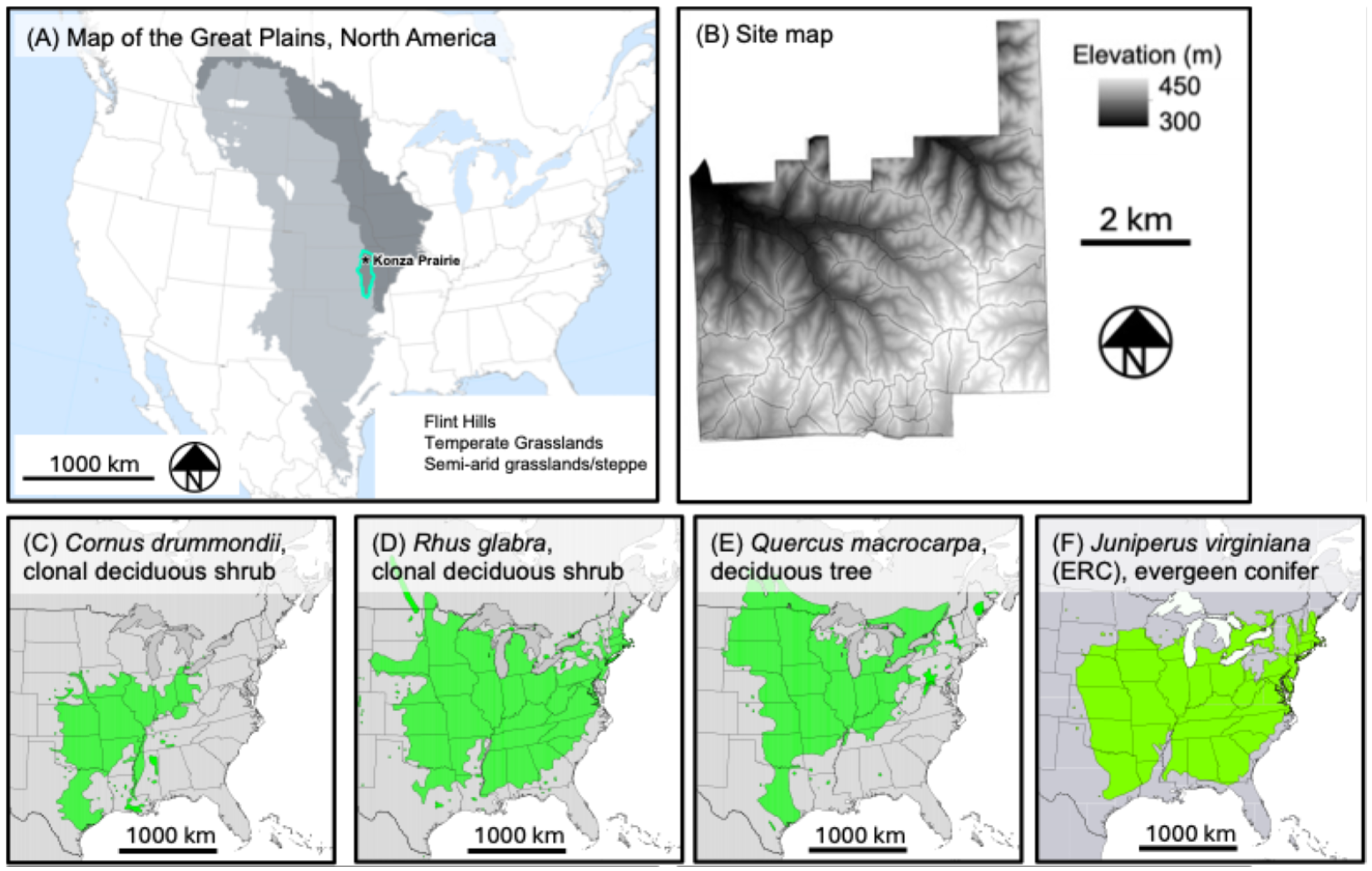
Our work took place at Konza Prairie Biological Station (KPBS), a National Science Foundation long-term ecological research (LTER) site with 3487 ha of native unplowed tallgrass prairie located in the Flint Hills in northeastern Kansas (Figure 1). The climate has high seasonal variability with an average high of 26.6 °C in July and −2.7 °C in January. Annual rainfall is 835 mm, with 75% falling during the growing season. The soils are non-glaciated with thin, rocky upland soils (mainly from the Florence series), deeper lowlands (often from the Tully series), and complex benches, outcrops, and slopes that connect these two soil types.
KPBS consists of 60 different management units, with replicates spanning 1-, 2-, 3-, 4-, and 20-year fire return intervals, as well as treatments ungrazed, grazed by bison, or grazed by cattle. These fire return intervals span the range found throughout the region [47]. The fire and grazing treatments have created a mosaic of contrasting land covers, including areas dominated by herbaceous species, shrubs, deciduous trees, and evergreen trees. The herbaceous-dominated areas can be floristically diverse, with high grass dominance in areas without bison or cattle, and mosaics of tallgrasses, short-grass grazing lawns, and patches of tall forbs in areas with bison and cattle [48]. Areas dominated by shrubs typically have minimal herbaceous cover [1,49]. The dominant shrubs (primarily the species Cornus drummondii, Rhus glabra, and Prunus americana) are all clonal, creating thickets with >10 m diameters. Shrub heights range from <0.5 m for young clonal stems to over 3 m for older stems [43]. At the lowest elevations and some intermittent streams, riparian forests have formed, dominated primarily by oaks (mostly Chinkapin oak, Quercus muehlenbergii and Bur oak, Quercus macrocarpa) [50]. Outside of these deepest lowlands, the height and continuity of deciduous trees are lower, with species including honeylocust (Gleditsia triacanthos), redbud (Cercis canadensis), and several elm species. ERC is the only evergreen native to the region, and primarily found in areas without bison or frequent fire. ERC is also one of the most widespread trees in North America, with a range that stretches from 100° W latitude in the west to the Atlantic Ocean in the east [51]. Figure 1B–E shows the widespread ranges of our most common encroaching species [51].

Figure 1.
(A) An estimate of the historical extent of arid and semi-arid Great Plains grasslands (light grey; based on U.S. EPA ecoregions), temperate Great Plains grasslands (dark grey; based on EPA ecoregions), the Flint Hills ecoregion (teal outline), and our study site (black star). (B) Shows an elevation map of our study site, Konza Prairie Biological Station. (C–F) show some of the range limits of some of the most dominant encroaching species. These include clonal shrubs (B,C), deciduous trees (D), and evergreen conifers, ERC (E). The base map for (A) is redrawn from EPA ecoregions Level II, and the base maps are from [51]. All are publicly available under a Creative Commons license.
2.2. Imagery
We tested each data source alone and together (NAIP + NEON) for a total of three models for each machine learning method, resulting in six models. Table 1 outlines the inputs used for each image, and Hulslander and colleagues [52] report formulas for vegetation indices. The images were captured in separate years: 2019 for NAIP and 2020 for NEON. Between these two years, there were no major weather fluctuations [48] or major fires, making significant changes in vegetation unlikely over this time period.

Table 1.
Summary of input variables and their descriptions used from each source.
NAIP imagery: We sourced this image from the USDA NAIP [53,54], which was captured on 10 July 2019 by low-flying planes. The native resolution was 0.6 × 0.6 m. We used bilinear interpolation to transform this image to a standard grid with 2 × 2 m pixels.
NAIP imagery contributed nine bands. The native imagery provided four bands (red, green, blue, and infrared), and we derived five more (red neighborhood, green neighborhood, blue neighborhood, infrared neighborhood, and NDVI; Table 1). Neighborhood calculations took the average value of all surrounding pixels. The red neighborhood calculation, for example, averaged the redness of the pixels immediately surrounding each pixel, including the diagonal neighbors (known as the “Queen’s rule”). We added neighborhood averages after early rounds of machine learning noticeably erroneously misclassified some deep shadows of shrubs and deciduous trees as ERC. Shadows are probably present because the image was taken later in the growing season than NEON, after full leaf-on.
NEON imagery: NSF NEON imagery was captured in June 2020 by low-flying airplanes and had a native resolution of 1 × 1 m, downloaded at [55,56]. Using bilinear interpolation, we upscaled these images to the same resolution and common grid as NAIP [57,58]. NEON provided many data products meant to capture the biophysical attributes of vegetation. For example, NDVI is calculated as the difference between near-infrared (NIR) and red bands, divided by the sum of NIR and red bands. We used eight derived vegetation indices from NEON: the Enhanced Vegetation Index (EVI), Normalized Difference Nitrogen Index (NDNI), Normalized Difference Lignin Index (NDLI), Soil-Adjusted Vegetation Index (SAVI), Atmospherically Resistant Vegetation Index (ARVI), NDVI, NDVI Neighborhood, and Canopy Height (LiDAR; Table 1). We included NDVI Neighborhood because this vegetation index was found in both datasets. We did not include Leaf Area Index because of its high overlap with SAVI. NEON’s 10 cm RGB was unusable for our purposes due to distortions along seamlines, but such distortions were not in the derived products. LiDAR data consisted of ~10 returns per m2, and canopy height was the top return per 1 × 1 m pixel. All other NEON indices were calculated using spectral data [52].
2.3. Machine Learning Methods
Machine learning uses a set of user inputs (training data) to learn and classify unknown data. We compared two supervised machine learning methods, SVMs and RFs, because they are commonly used in remote sensing and accessible to many users [33,59].
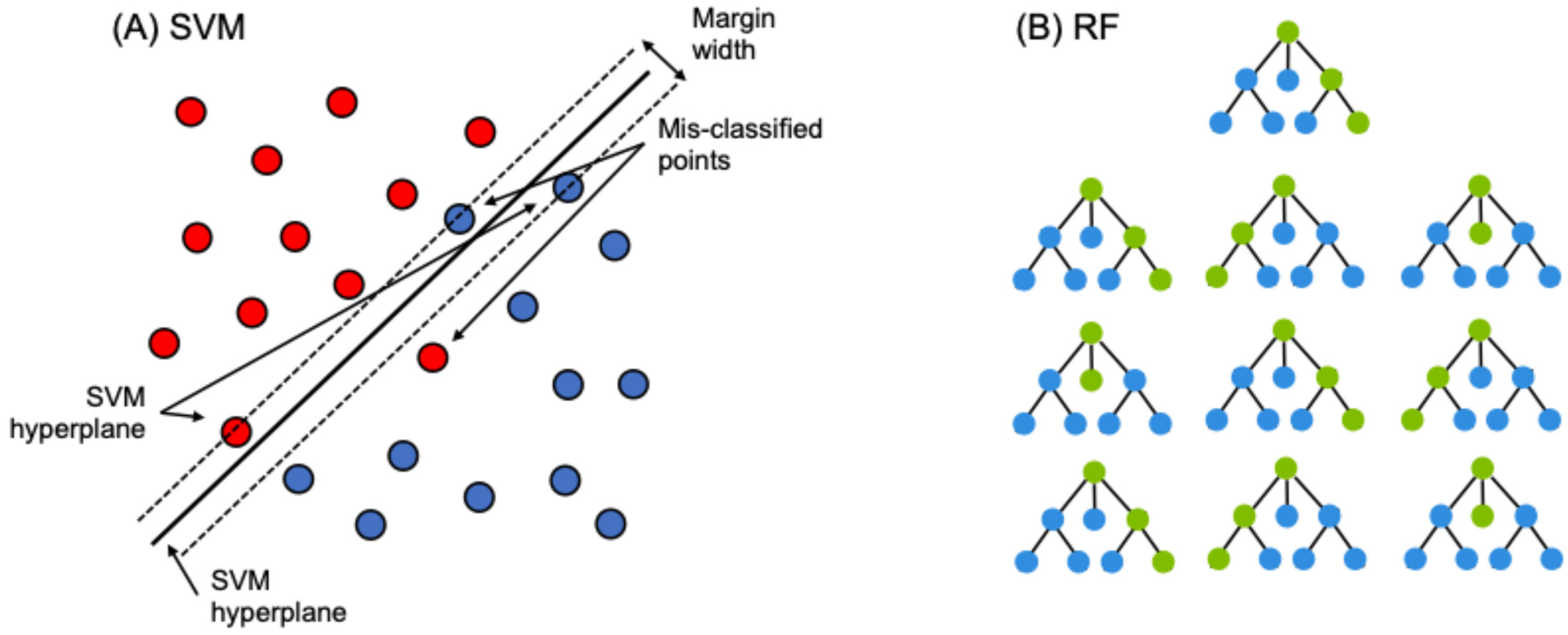
Support Vector Machines: SVMs are a supervised nonparametric classification model that uses a fixed optimal hyperplane to split data into discrete categories [60,61] (Figure 2A). SVMs are popular for their ability to work with high-dimensional data [59] and their accuracy even with small training sets relative to spatial extent [33,62].

Figure 2.
(A) We used a simple linear form of SVM like the one shown here (adapted from [60]). Each circle represents a training sample, where color denotes the land cover class. (B) A schematic of a random forest, where each decision tree is one of a “forest” of decision trees. Each circle and connecting line is decision node, defined by an “if statement” such as, “if Canopy height > 1.0 m, progress left on this branch, if <1.0 m progress right.”. Green connections show the progression of decisions made for the bootstrapped sample used to inform each tree. Note that we have kept the topology of each tree constant for this example, but in reality, the topology varies across trees. In this toy example, the random forest model would choose the left-most cover class as the predicted cover class.
In SVMs, each pixel is a series of numbers, with one value from each input, which are mapped with each input as a new dimension during SVM creation. Points closest to the hyperplane are support vectors and are the most important in determining the decision boundary. While many linear hyperplanes may exist in the data, SVM chooses the largest margin between points, allowing for some misclassification. Many datasets lack linear breaks between data, which SVMs can circumvent by shifting the data into a higher dimension using kernels. We ran SVMs in R [63] using the ‘e1071’ package. We determined model parameters using the ‘tune.svm’ function, considering input parameters spanning a range of degree 2 to 5, gamma 0.1–4, and cost of 1–3 [64]. This function performs 10-fold cross-validation, and we assumed used a radial kernel parameter in all cases. The final model parameters were NAIP (degree = 3, gamma = 0.1111, cost = 1), NEON (degree = 3, gamma = 0.1250, cost = 1), and NAIP + NEON (degree = 3, gamma = 0.0.0580, cost = 1).
Random Forest: RF is a nonparametric supervised machine learning technique that tends to have high accuracy and low out-of-bag error. The building block of RF is the decision tree, which uses nodes to split data into smaller subsets to predict the pixel class (much like multiple logistic regression). Examples are shown in Figure 2B. RFs use a bagging approach, where each decision tree is built with a random selection of input variables, creating a forest of different tree structures to limit overfitting [65]. The user can set the number of decision trees (ntree) and the number of input variables used to split each node (mtry), which is often approximately the square root of the number of inputs [33]. RFs make predictions based on majority voting; each decision tree outputs a predicted class for each pixel, and the class predicted the most times is the classification for that pixel (Figure 2B) [59]. For example, if an RF has 100 trees, and 56 trees predict a pixel as grassland, 33 trees predict shrubland, and 11 trees predict a deciduous tree, then the ensemble RF model would predict that pixel to be grassland. Adding more decision trees can improve accuracy, but an excessive number of trees yields diminishing returns in accuracy. Lastly, RF models can determine the GINI decrease for each input, which measures the amount of accuracy lost by an input variable, indicating the relative importance of each model input.
We ran RF models in R [63] using the ‘randomForest’ package, and model inputs were optimized using the ‘best.randomForest’ function, with an ntree range of 100 to 1000 and mtry of 1 to 5 [66]. Based on this tuning, we used an mtry of the 3 for the NAIP and NEON models, and an mtry of 4 for the NAIP + NEON model (mtry is the number of variables assessed at each decision tree node). For consistency, the number of trees was equal in all RF models, with an ntree of 500 (the number of trees in the RF).
2.4. Training Data
We considered five land cover categories: (1) grassland (herbaceous-dominated areas); (2) shrubs; (3) deciduous trees; (4) ERC trees; and (5) and other (roads, water, buildings, and agriculture). The training dataset consisted of ground-truth polygons collected using high-precision GPS units (<2 m accuracy) and computer-drawn polygons. We collected ground-truth polygons from June to August 2021 using semi-stratified random sampling. We created computer-drawn polygons by tracing vegetation types using a 2020 NEON RGB-10 cm imagery [67] and a publicly available 1 m2 RGB image from 2019 by Maxar technologies, accessed via Google Earth Pro [68]. Neither image was used in the model training. We drew polygons in locations where species were known from time in the field. We collected 3635 training polygons, with training proportions of each cover class reflecting estimated landscape cover, resulting in 300,328 2 × 2 m pixels of known vegetation type, totaling 3.42% of the study area (Table 2). Polygons were split into training and evaluation groups before being pixelized to reduce inflated accuracies due to spatial autocorrelation. We aimed to use 70% of the data for model training and 30% for model evaluation (sometimes referred to as model ‘validation’). After we separated the polygons into training and evaluation groups and then converted polygons into pixels, the proportion of training and evaluation pixels remained similar (71% and 29%, respectively).
Table 2.
Summary of training data. Training proportions are similar to landscape cover.
2.5. Assessing Accuracy
To assess the accuracy of each model, we considered four metrics: producer accuracy (PA), user accuracy (UA), overall accuracy (OA), and Kappa. PA refers to the number of pixels correctly classified from the evaluation data and was calculated as the number of correctly classified pixels for a class divided by the total number of evaluation pixels for that class. UA refers to the number of pixels classified as, for instance, grassland that were actually grassland on the ground (i.e., in the evaluation data). UA was calculated as the number of correctly classified pixels for a class divided by the total number of pixels assigned to that cover class. OA is an estimate of accuracy among all predicted cover types and was calculated as the ratio of the total number of correctly classified pixels to the total number of pixels in the evaluation data. Kappa measures the accuracies by comparing the classification outcome versus randomly assigning values. We calculated Kappa as (overall accuracy − random accuracy)/(1 − random accuracy). Kappa ranges from −1 to 1, with 0 indicating that the model performed the same randomly assigning values, <0 indicating that the model performed worse than random, and >0 indicating that the model performed better than random.
2.6. Run Time and Other Logistics
Run time is a consideration for some machine learning approaches. We reported run time for both model training and extrapolation to the remainder of our site (a total of 8,781,520 pixels). All models were run on a Dell XPS 8930 with relevant specifications of 64 GB RAM and an Intel® Core™ i9-9900K processor, with 3.6 GHz speed, eight cores, and the ability to perform 16 threads. Note that R runs most processes through the RAM and processor cores, including those used here. During runs, R was the only user-directed application open.
3. Results
3.1. Model Accuracy Overview
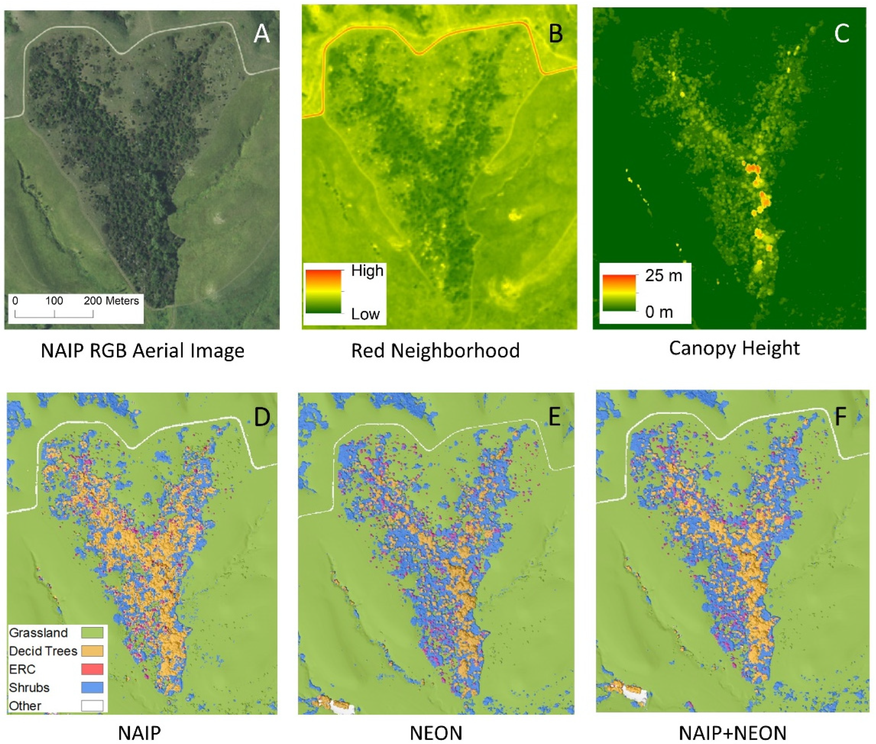
SVMs versus RFs yielded nearly identical OA (<2.6% difference; Table 3). NEON models generally performed better than NAIP, and the NAIP + NEON models were the most accurate. For NAIP-only models, RFs were slightly more accurate (OA: 92.9%, Kappa: 0.877) than SVMs (OA: 90.3%, Kappa: 0.831; Table 3). For NEON-only models, the accuracy of RFs (OA: 97.2%, Kappa: 0.951) and SVMs was similar (OA: 96.8%, Kappa: 0.945; Table 3). NAIP + NEON models showed effectively no differences between RFs (OA: 97.7%, Kappa: 0.962) and SVMs (OA: 97.7%, Kappa: 0.964; Table 3). Figure 3D,E show classified vegetation maps comparing all three data sources, where the machine learning method was RF for all panels.
Table 3.
Accuracy results of all image and machine learning methods.
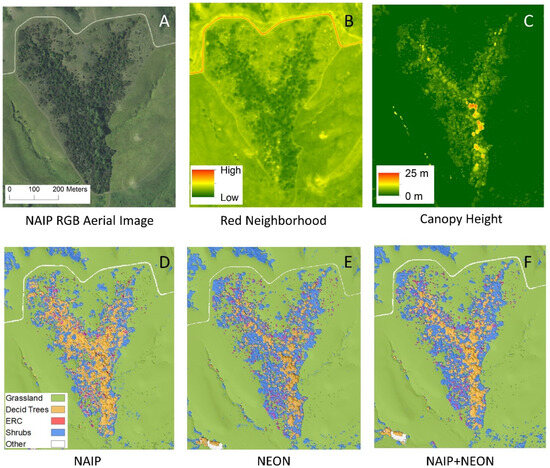
Figure 3.
A small portion of the study area, zoomed in to show detail: (A) aerial imagery from NAIP RGB (red–green–blue; naked eye view); (B) visual of values in most important NAIP input for model training; (C) visual of values in most important NEON input for model training; (D–F) visuals of RF-classified models for all three images.
For all models, the grassland and “other” categories had UA and PA values of at least 94% (Table 3). The three categories of woody plants (shrubs, deciduous trees, and ERC) were more difficult to classify but still had high accuracy ratings. Shrubs and deciduous trees had very high PA and UA accuracies (>92%) in NEON and NAIP + NEON, but NAIP alone performed slightly worse, with a PA of 85–93% for shrubs and 72–77% for deciduous trees and a UA of 82–85% for shrubs and 89–92% for deciduous trees (Table 3). Deciduous trees were most often misclassified as shrubs, and shrubs were most often misclassified as deciduous trees (Table 4, Table 5 and Table 6). All models had the lowest accuracies for ERC (Table 3), especially the NAIP-only models, with PAs of 52–56% and UAs of 75–78% (Table 4). This low PA means that the models are undercounting ERC by classifying it as another cover class (mostly deciduous trees), rather than misclassifying other categories as ERC (also referred to as errors of commission) (Table 4 and Table 5). Most of these errors were ERC pixels classified as deciduous trees (Table 4, Table 5 and Table 6).
Table 4.
Confusion matrix for NAIP-only models, starting with SVMs and followed by RFs; columns represent the classes of evaluation pixels, and rows represent the classes of model classified pixels *.
Table 5.
Confusion matrix for NEON-only models, starting with SVMs and followed by RFs; columns represent the classes of evaluation pixels, and rows represent the classes of model-classified pixels *.
Table 6.
Confusion matrix for NAIP + NEON models, starting with SVMs and followed by RFs; columns represent the classes of evaluation pixels, and rows represent the classes of model classified pixels *.
3.2. Importance of Different Imagery Data Inputs
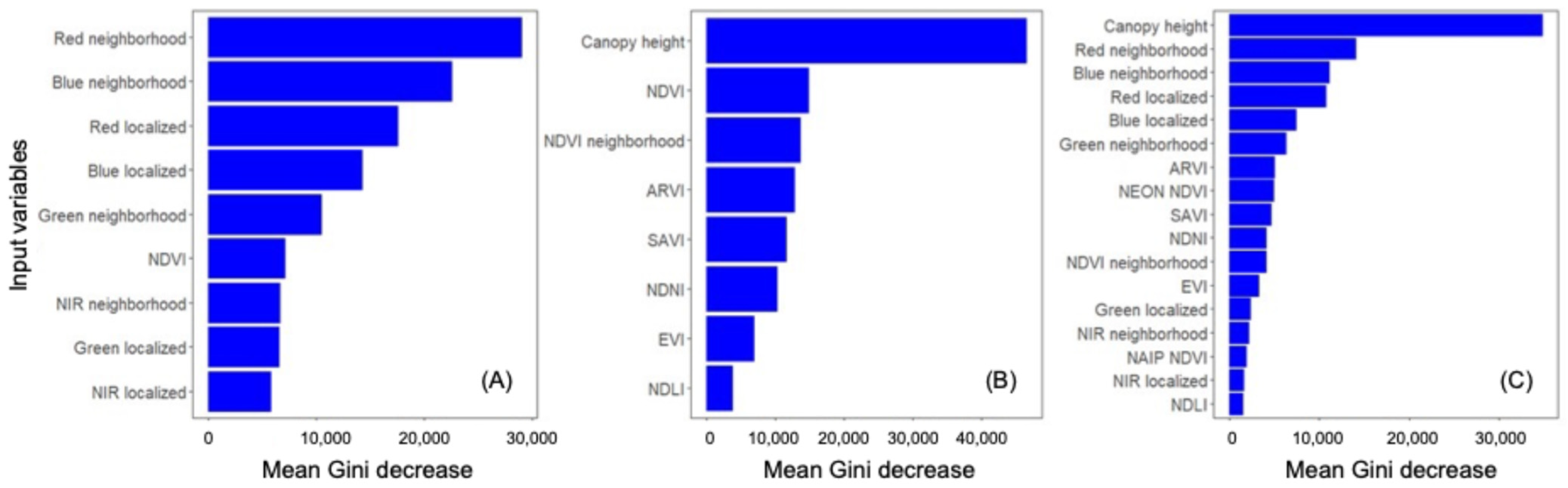
For NAIP, the most valuable input variable was red neighborhood (visualized in Figure 3B), followed by blue neighborhood and red and blue light intensity (Figure 4A). NDVI was effectively tied with three other variables for the lowest contribution to this model’s accuracy. The most valuable input variable for NEON was canopy height (visualized in Figure 3C), followed far behind by NDVI and NDVI neighborhood (Figure 4B). The commonly used EVI had the second-lowest contribution to model accuracy. The NAIP + NEON RF also relied heavily on LiDAR, followed by five inputs from NAIP: red neighborhood, blue neighborhood, red localized, blue localized, and green neighborhood. In the combined model, NEON-derived products other than canopy height provided very minimal contributions to model accuracy (Figure 4C).
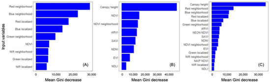
Figure 4.
Average importance of each variable in Random Forest model building for: (A) NAIP-only, (B) NEON-only, and (C) NAIP and NEON together. Mean Gini decrease measures the accuracy lost when that variable is removed. See Table 1 for input definitions.
3.3. Model Run Time and Other Logistics
The time it took to train each model on the training data varied greatly, with the shortest time at only 23 min for RF NEON, and the longest at 4 h and 49 min for SVM NAIP (Table 7). RF and SVM models had substantial differences between training run times; the slowest RF model still took less time (1 h and 5 min) than the fastest SVM model (1 h and 37 min) (Table 7). The time it took the models to predict the entire study site (8,781,520 pixels) was again substantially lower for RFs at 7:20–10:43 min, whereas SVM classification took 2:05–6:15 h (Table 7).
Table 7.
Run times for model training and prediction.
4. Discussion
Until recently, NAIP was the primary high-resolution, freely available, widely available source of aerial remote sensing in the U.S.A. [36]. We found that with a few manipulations (use of neighborhoods) and readily available machine learning methods, NAIP imagery succeeded at identifying grasslands, shrubs, and deciduous trees. NEON [55,56] substantially increased our ability to accurately identify all forms of woody vegetation, especially ERC. NEON imagery also made classification less subject to the type of machine learning model. NEON-derived increases in accuracy were due to LiDAR canopy height, with spectral data from NAIP providing much of the remaining contributions to model accuracy. Therefore, in the locations where NEON imagery is available (81 total sites), the two data sources could be used synergistically—NEON for its LiDAR and NAIP for its undistorted red, green, blue, and NIR. The addition of LiDAR to NAIP coverage, where possible, could bolster remote sensing of WPE, considering that our best-performing models had very high accuracy: >99.1% for grasslands, 98.1% for shrubs, 94.8% for deciduous trees, 85.3% for ERC, and 98.5% for other (Table 6).
Challenges and success in remote sensing WPE: Differences in deciduous versus evergreen functional types are a fundamental divide in tree functional types. We hypothesized that ERC would have much higher accuracy due to its distinct leaf structure and water content compared to other woody plants in the region. These characteristics should theoretically register in NEON-derived products (e.g., NDVI, NDLI, NDNI). However, ERC had the lowest accuracy in all models and was often undercounted, in some cases by almost half (Table 4, Table 5 and Table 6). This problem was acute when we only used NAIP imagery (Table 4). Other studies also had difficulty detecting ERC in aerial imagery, specifically when ERC was at a low density [69,70]. At densities below 30%, Kaskie and colleagues [69] found <50% accuracy in ERC classification using aerial imagery alone—very similar to our NAIP-only models (Table 4). However, using other predictor variables, such as slope, aspect, and Euclidean distance, to the nearest ERC pixel, Kaskie and colleagues [70] were able to increase the overall accuracy of low-density ERC to 84.7%. ERC density was also low across our site, but accuracy was high (78–94%; Table 3) in models including NEON data. Therefore, NEON and its LiDAR appear to overcome some challenges of low-density ERC detection and, presumably, other evergreen tree species. However, more work is needed to determine better and more efficient methods to accurately classify ERC and similar evergreen trees at low densities. For instance, ERC might need to be a higher proportion of the training data, even if it is a relatively rare cover class across a landscape. Winter imagery could be especially helpful for boosting ERC detection.
LiDAR substantially increased the accuracy of detecting shrubs and deciduous trees. Models with LiDAR were more accurate and LiDAR canopy height was by far the most influential input for RF models (Figure 4). This is consistent with many other studies finding that LiDAR-based canopy height was among the most important inputs for accurately classifying vegetation types, including separating woody plants from herbaceous plants and differentiating between species of trees [71,72,73]. For instance, Jin and Mountrakis [74] analyzed 37 studies that compared accuracy using multispectral imagery alone versus classification with LiDAR added and found increases in model accuracy for almost all studies, including a 68% increase in one study. This again points toward value added from NEON, but specifically from the addition of LiDAR, as NEON vegetation indices other than canopy height played a minor role in increasing model accuracy in the NAIP + NEON model (Figure 4). NEON also provides a full suite of hyperspectral data, which we did not test but could have yet more value added.
Shrubs and small trees have been difficult to classify in the past because they are often smaller than the resolution of remotely sensed aerial imagery [75], leading to undercounting of shrubs and small trees [39]. For instance, even sophisticated machine learning approaches can yield overall accuracies as low as 48% for shrubs (e.g., [76]) or as high as 88% when high-resolution data are available and shrubs sharply contrast with surrounding vegetation (e.g., [77]). It is also not uncommon for shrubs to be combined with herbaceous vegetation as a potential class (e.g., [78]), reflecting the difficulties of separating herbaceous species and shrubs. Thus, we hypothesized that shrubs would be our lowest accuracy cover class. However, we found high accuracy for shrubs in all models (Table 3). Some of this success may be because the most common encroaching species—C. drummondii—can produce high Leaf Area Index values, with taller shrubs reaching values typical of dense deciduous or tropical forests [43]. Foliar nitrogen of woody species in this ecosystem is also high [79] compared to the surrounding herbaceous vegetation [44]. It remains unclear whether the data sources and methods we used would perform as well in grasslands with WPE by shorter, less dense species or grassland matrices with taller, more nutrient-rich swards. Nonetheless, this study is in the relative minority of succeeding at high-resolution remote sensing of shrubs in high-productivity ecosystems [28,38,80].
Machine learning methods: We found that two commonly used machine learning techniques achieved similar accuracy, except in some specific cases, such as remote sensing of conifers without LiDAR data. RF models added a small amount of accuracy (<2.6%), but the larger difference was that RFs ran substantially faster than SVM models in R (Table 7). While the differences in run time meant that most models could train a machine learning model and project it to our study site in one day, run time would become an issue at larger spatial extents and over multiple time periods. RF was also slightly less sensitive to the data source, whereas SVMs’ performance suffered when using only NAIP imagery. RFs also have the advantage of easily parsing the importance of different input variables, which is valuable for the synergistic use of multiple remote sensing platforms. These observations come with the caveat that all analyses were run using common packages in R, with no substantial effort to optimize run time. Run times will likely differ based on the packages used or if run in a different coding environment. For computer specifications, see the methods section.
Accessibility of high-resolution remote sensing remote sensing: Remote sensing now has many options, such as UAVs, planes, and a growing suite of public and private satellites. Others have already reviewed the relative advantages of each approach in depth [35,81,82,83,84]. Generally, the advantages of low-flying planes, including the ones used here, fall between UAVs and state-run satellites, with a greater spatial extent than most UAVs and finer spatial resolution (grain) than most satellites. Low-flying planes can easily carry heavy payloads, including hyperspectral cameras and high-return high-resolution LiDAR (e.g., [29,40]). The typical disadvantage of remote sensing via planes is the initial learning curve and expense of piloting planes, maintaining equipment under flight conditions, and data cleaning/carpentry. These limitations also mean that remote sensing from low-flying planes often has lower temporal resolution. For instance, NAIP images are typically available every two years [36], whereas user-based drones and most satellites provide multiple measurements per growing season [35,81].
Publicly supported platforms have negated some disadvantages of low-flying planes by concentrating expertise. Experienced pilots and technologists capture the data. Skilled data scientists then perform the initial data cleaning and formatting. The result is data in a format familiar to most end-users (e.g., a raster in ‘.tif’ format), often free of distortions such as cloud cover, significant spectral changes due to weather, and seamlines. This specialization reduces many of the logistical and financial barriers to using high-resolution data for image classification—a key part of the stated goals of state and federal programs to democratize scientific pursuits [36,37]. At a minimum, our results suggest that publicly available imagery can provide proof of concept to motivate more involved approaches such as UAVs or proprietary satellites. In some ecosystems, such as tallgrass prairie and similar ecosystems, our results suggest that publicly available imagery can track vegetation transitions, such as WPE. Similarly, contemporary and historical aerial imagery from planes has been used to remote sense woody vegetation [40,45,84,85] and WPE before [8,18,19,23,27,28,38,80,86,87]. The difference is that most of these studies using plane-based data were from ad hoc imagery. In contrast, one of the sources we use here is available nationwide in the U.S.A.—USDA NAIP [36]. The other is available for at least one site for each of North America’s most widespread terrestrial ecosystem types—NEON AOP [37]. We were privileged to have such a wealth of publicly available data, and therefore, echo hopes that similar data become widely available [88].
5. Conclusions
Management of woody plant encroachment, including clonal shrublands and ERC trees, is costly and time-consuming. Early detection of small individual shrubs and trees can allow managers to engage in preventative management while woody plants are still at low densities and less resistant to disturbances, such as fire. More accurate remote sensing can help with biodiversity and ecosystem service assessments. We found that two imagery sources resulted in accurate detection of major forms of WPE, with especially large increases in accuracy with the addition of LiDAR. Our results suggest that this type of tracking could succeed in similar ecosystems with relatively low upfront effort and cost, enabling the adaptive management of biodiversity, ecosystem services, and environmental resilience.
Author Contributions
Conceptualization, Methodology, Software, Validation, Data curation, B.N. and Z.R.; Writing—original draft, B.N. and Z.R.; Writing—review & editing, B.N. and Z.R. All authors have read and agreed to the published version of the manuscript.
Funding
This work and the authors were supported by Konza Prairie LTER (U.S.A. National Science Foundation award DEB #2025849), the EPSCoR MAPS program (U.S.A. National Science Foundation award #1656006), the Kansas State University Agricultural Experimental Station, and the Kansas State University Division of Biology.
Data Availability Statement
Data sets utilized for this research are as follows: Noble, B. and Z. Ratajczak. 2022. WPE01 Assessing the value added of NEON for using machine learning to quantify vegetation mosaics and woody plant encroachment at Konza Prairie ver 1. Environmental Data Initiative. https://doi.org/10.6073/pasta/a7b40e41080460bb1123dcc7b6d4d942 (Accessed on 8 December 2022). https://portal.edirepository.org/nis/mapbrowse?scope=knb-lter-knz&identifier=167&revision=1 (Accessed on 1 May 2025). Code is at Figshare via the following link: https://figshare.com/s/9d0f3ae0f13385109551 (Accessed on 1 May 2025).
Acknowledgments
We thank the many pilots, technicians, programmers, and support staff who capture and make accessible data from the NAIP and NEON aerial observations programs. We thank the U.S. Department of Agriculture (USDA) and the U.S. National Science Foundation for funding the capture of the aerial imagery, which was vital to this study. We thank the many staff, students, faculty, and volunteers who have maintained the fire and grazing treatments at Konza Prairie Biological Station, which were integral to this study. Dylan Darter, Chase Glasscock, Sidney Noble, and Jaclyn Perry contributed to the study. We thank Trimble for purchase of high-accuracy GPS units with an educational discount. Contribution no. 25-228-J from the Kansas Agricultural Experiment Station.
Conflicts of Interest
The authors declare no conflicts of interest.
References
- Briggs, J.M.; Knapp, A.K.; Blair, J.M.; Heisler, J.L.; Hoch, G.A.; Lett, M.S.; McCarron, J.K. An ecosystem in transition: Causes and consequences of the conversion of mesic grassland to shrubland. BioScience 2005, 55, 243–254. [Google Scholar] [CrossRef]
- Brandt, J.S.; Haynes, M.A.; Kuemmerle, T.; Waller, D.M.; Radeloff, V.C. Regime shift on the roof of the world: Alpine meadows converting to shrublands in the southern Himalayas. Biol. Conserv. 2013, 158, 116–127. [Google Scholar] [CrossRef]
- Moser, W.K.; Hansen, M.H.; Atchison, R.L.; Butler, B.J.; Crocker, S.J.; Domke, G.; Kurtz, C.M.; Lister, A.; Miles, P.D. Kansas’ forests 2010. In Resource Bulletin; NRS-85; USDA Forest Service, Northern Research Station: Newtown Square, PA, USA, 2013; Volume 63. [Google Scholar]
- Twidwell, D.; Rogers, W.E.; Fuhlendorf, S.D.; Wonkka, C.L.; Engle, D.M.; Weir, J.R.; Kreuter, U.P.; Taylor, C.A. The rising Great Plains fire campaign: Citizens’ response to woody plant encroachment. Front. Ecol. Environ. 2013, 11 (Suppl. S1), e64–e71. [Google Scholar] [CrossRef]
- Galgamuwa, G.P.; Wang, J.; Barden, C.J. Expansion of Eastern Redcedar (Juniperus virginiana L.) into the Deciduous Woodlands within the Forest–Prairie Ecotone of Kansas. Forests 2020, 11, 154. [Google Scholar] [CrossRef]
- Archer, S.R.; Andersen, E.M.; Predick, K.I.; Schwinning, S.; Steidl, R.J.; Woods, S.R. Woody plant encroachment: Causes and consequences. In Rangeland Systems: Processes, Management and Challenges; Springer: Berlin/Heidelberg, Germany, 2017; pp. 25–84. [Google Scholar]
- Brunsell, N.A.; Van Vleck, E.S.; Nosshi, M.; Ratajczak, Z.; Nippert, J.B. Assessing the roles of fire frequency and precipitation in determining woody plant expansion in central US grasslands. J. Geophys. Res. Biogeosci. 2017, 122, 2683–2698. [Google Scholar] [CrossRef]
- Nippert, J.B.; Ocheltree, T.W.; Orozco, G.L.; Ratajczak, Z.; Ling, B.; Skibbe, A.M. Evidence of physiological decoupling from grassland ecosystem drivers by an encroaching woody shrub. PLoS ONE 2013, 8, e81630. [Google Scholar] [CrossRef]
- Miller, J.E.; Damschen, E.I.; Ratajczak, Z.; Özdoğan, M. Holding the line: Three decades of prescribed fires halt but do not reverse woody encroachment in grasslands. Landsc. Ecol. 2017, 32, 2297–2310. [Google Scholar] [CrossRef]
- Collins, S.L.; Nippert, J.B.; Blair, J.M.; Briggs, J.M.; Blackmore, P.; Ratajczak, Z. Fire frequency, state change and hysteresis in tallgrass prairie. Ecol. Lett. 2021, 24, 636–647. [Google Scholar] [CrossRef]
- Ratajczak, Z.; D’Odorico, P.; Nippert, J.B.; Collins, S.L.; Brunsell, N.A.; Ravi, S. Changes in spatial variance during a grassland to shrubland state transition. J. Ecol. 2017, 105, 750–760. [Google Scholar] [CrossRef]
- Ratajczak, Z.; D’Odorico, P.; Collins, S.L.; Bestelmeyer, B.T.; Isbell, F.I.; Nippert, J.B. The interactive effects of press/pulse intensity and duration on regime shifts at multiple scales. Ecol. Monogr. 2017, 87, 198–218. [Google Scholar] [CrossRef]
- Swengel, A.B. Effects of fire and hay management on abundance of prairie butterflies. Biol. Conserv. 1996, 76, 73–85. [Google Scholar] [CrossRef]
- Lettow, M.C.; Brudvig, L.A.; Bahlai, C.A.; Gibbs, J.; Jean, R.P.; Landis, D.A. Bee community responses to a gradient of oak savanna restoration practices. Restor. Ecol. 2018, 26, 882–890. [Google Scholar] [CrossRef]
- Engle, D.M.; Coppedge, B.R.; Fuhlendorf, S.D. From the dust bowl to the green glacier: Human activity and environmental change in Great Plains grasslands. In Western North American Juniperus Communities; Springer: New York, NY, USA, 2008; pp. 253–271. [Google Scholar]
- Silber, K.M.; Hefley, T.J.; Castro-Miller, H.N.; Ratajczak, Z.; Boyle, W.A. The long shadow of woody encroachment: An integrated approach to modeling grassland songbird habitat. Ecol. Appl. 2024, 34, e2954. [Google Scholar] [CrossRef] [PubMed]
- Lautenbach, J.M.; Plumb, R.T.; R.n, S.G.; Hagen, C.A.; Haukos, D.A.; Pitman, J.C. Lesser prairie-chicken avoidance of trees in a grassland landscape. Rangel. Ecol. Manag. 2017, 70, 78–86. [Google Scholar] [CrossRef]
- Albrecht, M.A.; Becknell, R.E.; Long, Q. Habitat change in insular grasslands: Woody encroachment alters the population dynamics of a rare ecotonal plant. Biol. Conserv. 2016, 196, 93–102. [Google Scholar] [CrossRef]
- Keen, R.M.; Nippert, J.B.; Sullivan, P.L.; Ratajczak, Z.; Ritchey, B.; O’Keefe, K.; Dodds, W.K. Impacts of Riparian and Non-riparian Woody Encroachment on Tallgrass Prairie Ecohydrology. Ecosystems 2022, 26, 290–301. [Google Scholar] [CrossRef]
- Dodds, W.K.; Ratajczak, Z.; Keen, R.M.; Nippert, J.B.; Grudzinski, B.; Veach, A.; Taylor, J.H.; Kuhl, A. Trajectories and state changes of a grassland stream and riparian zone after a decade of woody vegetation removal. Ecol. Appl. 2023, 33, e2830. [Google Scholar] [CrossRef]
- Morford, S.L.; Allred, B.W.; Twidwell, D.; Jones, M.O.; Maestas, J.D.; Roberts, C.P.; Naugle, D.E. Herbaceous production lost to tree encroachment in United States rangelands. J. Appl. Ecol. 2022, 59, 2971–2982. [Google Scholar] [CrossRef]
- Ratajczak, Z.; Nippert, J.B.; Briggs, J.M.; Blair, J.M. Fire dynamics distinguish grasslands, shrublands and woodlands as alternative attractors in the Central Great Plains of North America. J. Ecol. 2014, 102, 1374–1385. [Google Scholar] [CrossRef]
- Meneguzzo, D.M.; Liknes, G.C. Status and Trends of Eastern Redcedar (Juniperus virginiana) in the Central United States: Analyses and Observations Based on Forest Inventory and Analysis Data. J. For. 2015, 113, 325–334. [Google Scholar] [CrossRef]
- Briggs, J.; Hoch, G.; Johnson, L. Assessing the Rate, Mechanisms, and Consequences of the Conversion of Tallgrass Prairie to Juniperus virginiana Forest. Ecosystems 2002, 5, 578–586. [Google Scholar] [CrossRef]
- Ratajczak, Z.; Briggs, J.M.; Goodin, D.G.; Luo, L.; Mohler, R.L.; Nippert, J.B.; Obermeyer, B. Assessing the potential for transitions from tallgrass prairie to woodlands: Are we operating beyond critical fire thresholds? Rangel. Ecol. Manag. 2016, 69, 280–287. [Google Scholar] [CrossRef]
- Loss, S.R.; Noden, B.H.; Fuhlendorf, S.D. Woody plant encroachment and the ecology of vector-borne diseases. J. Appl. Ecol. 2022, 59, 420–430. [Google Scholar] [CrossRef]
- Veach, A.M.; Dodds, W.K.; Skibbe, A. Fire and grazing influences on rates of riparian woody plant expansion along grassland streams. PLoS ONE 2014, 9, e106922. [Google Scholar] [CrossRef]
- Laliberte, A.S.; Rango, A.; Havstad, K.M.; Paris, J.F.; Beck, R.F.; McNeely, R.; Gonzalez, A.L. Object-oriented image analysis for mapping shrub encroachment from 1937 to 2003 in southern New Mexico. Remote Sens. Environ. 2004, 93, 198–210. [Google Scholar] [CrossRef]
- Asner, G.P.; Knapp, D.E.; Boardman, J.; Green, R.O.; Kennedy-Bowdoin, T.; Eastwood, M.; Martin, R.E.; Anderson, C.; Field, C.B. Carnegie Airborne Observatory-2: Increasing science data dimensionality via high-fidelity multi-sensor fusion. Remote Sens. Environ. 2012, 124, 454–465. [Google Scholar] [CrossRef]
- Allred, B.W.; Bestelmeyer, B.T.; Boyd, C.S.; Brown, C.; Davies, K.W.; Duniway, M.C.; Ellsworth, L.M.; Erickson, T.A.; Fuhlendorf, S.D.; Griffiths, T.V.; et al. Improving Landsat predictions of rangeland fractional cover with multitask learning and uncertainty. Methods Ecol. Evol. 2021, 12, 841–849. [Google Scholar] [CrossRef]
- Kranjčić, N.; Medak, D.; Župan, R.; Rezo, M. Support vector machine accuracy assessment for extracting green urban areas in towns. Remote Sens. 2019, 11, 655. [Google Scholar] [CrossRef]
- Nguyen, H.T.T.; Doan, T.M.; Tomppo, E.; McRoberts, R.E. Land Use/land cover mapping using multitemporal Sentinel-2 imagery and four classification methods—A case study from Dak Nong, Vietnam. Remote Sens. 2020, 12, 1367. [Google Scholar] [CrossRef]
- Thanh Noi, P.; Kappas, M. Comparison of Random Forest, k-Nearest Neighbor, and Support Vector Machine Classifiers for Land Cover Classification Using Sentinel-2 Imagery. Sensors 2018, 18, 18. [Google Scholar] [CrossRef]
- Freitag, M.; Kamp, J.; Dara, A.; Kuemmerle, T.; Sidorova, T.V.; Stirnemann, I.A.; Velbert, F.; Hölzel, N. Post-soviet shifts in grazing and fire regimes changed the functional plant community composition on the Eurasian steppe. Glob. Change Biol. 2021, 27, 388–401. [Google Scholar] [CrossRef] [PubMed]
- Toth, C.; Jóźków, G. Remote sensing platforms and sensors: A survey. ISPRS J. Photogramm. Remote Sens. 2016, 115, 22–36. [Google Scholar] [CrossRef]
- Maxwell, A.E.; Warner, T.A.; Vanderbilt, B.C.; Ramezan, C.A. Land Cover Classification and Feature Extraction from National Agriculture Imagery Program (NAIP) Orthoimagery: A Review. Photogramm. Eng. Remote Sens. 2017, 83, 737–747. [Google Scholar] [CrossRef]
- Nagy, R.C.; Balch, J.K.; Bissell, E.K.; Cattau, M.E.; Glenn, N.F.; Halpern, B.S.; Ilangakoon, N. Harnessing the NEON data revolution to advance open environmental science with a diverse and data-capable community. Ecosphere 2021, 12, e03833. [Google Scholar] [CrossRef]
- Soubry, I.; Guo, X. Quantifying woody plant encroachment in grasslands: A review on remote sensing approaches. Can. J. Remote Sens. 2022, 48, 337–378. [Google Scholar] [CrossRef]
- Brandt, M.; Tucker, C.J.; Kariryaa, A.; Rasmussen, K.; Abel, C.; Small, J.; Chave, J.; Rasmussen, L.V.; Hiernaux, P.; Diouf, A.A.; et al. An unexpectedly large count of trees in the West African Sahara and Sahel. Nature 2020, 587, 78–82. [Google Scholar] [CrossRef] [PubMed]
- Baldeck, C.A.; Asner, G.P.; Martin, R.E.; Anderson, C.B.; Knapp, D.E.; Kellner, J.R.; Wright, S.J. Operational tree species mapping in a diverse tropical forest with airborne imaging spectroscopy. PLoS ONE 2015, 10, e0118403. [Google Scholar] [CrossRef] [PubMed]
- Griffith, D.M.; Byrd, K.B.; Anderegg, L.D.; Allan, E.; Gatziolis, D.; Roberts, D.; Yacoub, R.; Nemani, R.R. Capturing patterns of evolutionary relatedness with reflectance spectra to model and monitor biodiversity. Proc. Natl. Acad. Sci. USA 2023, 120, e2215533120. [Google Scholar] [CrossRef]
- Pau, S.; Nippert, J.B.; Slapikas, R.; Griffith, D.; Bachle, S.; Helliker, B.R.; O’Connor, R.C.; Riley, W.J.; Still, C.J.; Zaricor, M. Poor relationships between NEON Airborne Observation Platform data and field-based vegetation traits at a mesic grassland. Ecology 2022, 103, e03590. [Google Scholar] [CrossRef]
- Tooley, E.G.; Nippert, J.B.; Ratajczak, Z. Evaluating methods for measuring the leaf area index of encroaching shrubs in grasslands: From leaves to optical methods, 3-D scanning, and airborne observation. Agric. For. Meteorol. 2024, 349, 109964. [Google Scholar] [CrossRef]
- Klodd, A.E.; Nippert, J.B.; Ratajczak, Z.; Waring, H.; Phoenix, G.K. Tight coupling of leaf area index to canopy nitrogen and phosphorus across heterogeneous tallgrass prairie communities. Oecologia 2016, 182, 889–898. [Google Scholar] [CrossRef]
- Weinstein, B.G.; Marconi, S.; Zare, A.; Bohlman, S.A.; Singh, A.; Graves, S.J.; Magee, L.; Johnson, D.J.; Record, S.; Rubio, V.E.; et al. Individual canopy tree species maps for the National Ecological Observatory Network. PLoS Biol. 2024, 22, e3002700. [Google Scholar] [CrossRef]
- Wedel, E.R.; Ratajczak, Z.; Tooley, E.G.; Nippert, J.B. Divergent resource-use strategies of encroaching shrubs: Can traits predict encroachment success in tallgrass prairie? J. Ecol. 2025, 113, 339–352. [Google Scholar] [CrossRef]
- Scholtz, R.; Prentice, J.; Tang, Y.; Twidwell, D. Improving on MODIS MCD64A1 burned area estimates in grassland systems: A case study in Kansas Flint Hills tall grass prairie. Remote Sens. 2020, 12, 2168. [Google Scholar] [CrossRef]
- Ratajczak, Z.; Collins, S.L.; Blair, J.M.; Nippert, J.B. Reintroducing bison results in long-running and resilient increases in grassland diversity. Proc. Natl. Acad. Sci. USA 2022, 119, e2210433119. [Google Scholar] [CrossRef]
- Ratajczak, Z.; Nippert, J.B.; Hartman, J.C.; Ocheltree, T.W. Positive feedbacks amplify rates of woody encroachment in mesic tallgrass prairie. Ecosphere 2011, 2, 121. [Google Scholar] [CrossRef]
- VanderWeide, B.L.; Hartnett, D.C. Fire resistance of tree species explains historical gallery forest community composition. For. Ecol. Manag. 2011, 261, 1530–1538. [Google Scholar] [CrossRef]
- Thompson, R.S.; Anderson, K.H.; Bartlein, P.J. Digital representations of tree species range maps from “Atlas of United States trees” by Elbert L. Little, Jr. (and other publications). In Atlas of Relations Between Climatic Parameters and Distributions of Important Trees and Shrubs in North America; U.S. Geological Survey, Information Services (Producer): Denver, CO, USA, 1999; On file at: U.S. Department of Agriculture, Forest Service, Rocky Mountain Research Station, Fire Sciences Laboratory: Missoula, MT, USA; FEIS files. [82831]. [Google Scholar]
- Hulslander, D. NEON Normalized Difference Vegetation Index (NDVI), Enhanced Vegetation Index (EVI), Atmospherically Resistant Vegetation Index (ARVI), Canopy Xanthophyll Cycle (PRI), and Canopy Lignin (NDLI) Algorithm Theoretical Basis Document (NEON Doc. #: NEON.DOC.002391, Rev. A). NEON Inc. 2016. Available online: https://data.neonscience.org/data-products/DP3.30026.001 (accessed on 26 May 2025).
- USDA Geospatial Data Gateway. NAIP Orthorectified Kansas Color Infrared 161 2019. Available online: https://nrcs.app.box.com/v/naip/file/579854034024 (accessed on 1 November 2020).
- USDA Geospatial Data Gateway. NAIP Orthorectified Kansas Natural Color 161 2019. Available online: https://nrcs.app.box.com/v/naip/file/578936034378 (accessed on 1 November 2020).
- NEON (National Ecological Observatory Network). Ecosystem structure (DP3.30015.001) 2020. RELEASE-2022. Available online: https://data.neonscience.org (accessed on 8 December 2022). [CrossRef]
- NEON (National Ecological Observatory Network). Vegetation indices—Spectrometer—Mosaic (DP3.30026.001) 2020. RELEASE-2022. Available online: https://data.neonscience.org (accessed on 8 December 2022). [CrossRef]
- Noble, B.; Ratajczak, Z. WPE01 Assessing the value added of NEON for using machine learning to quantify vegetation mosaics and woody plant encroachment at Konza Prairie ver 1. Environ. Data Initiat. 2022. [Google Scholar] [CrossRef]
- Noble, B.; Ratajczak, Z. Combining machine learning and publicly available aerial data (NAIP and NEON) to achieve high-resolution remote sensing of grass-shrub-tree mosaics in the Central Great Plains (USA). bioRxiv 2025. [Google Scholar] [CrossRef]
- Sheykhmousa, M.; Mahdianpari, M.; Ghanbari, H.; Mohammadimanesh, F.; Ghamisi, P.; Homayouni, S. Support vector machine versus random forest for remote sensing image classification: A meta-analysis and systematic review. IEEE J. Sel. Top. Appl. Earth Obs. Remote Sens. 2020, 13, 6308–6325. [Google Scholar] [CrossRef]
- Burges, C.J. A tutorial on support vector machines for pattern recognition. Data Min. Knowl. Discov. 1998, 2, 121–167. [Google Scholar] [CrossRef]
- Mountrakis, G.; Im, J.; Ogole, C. Support vector machines in remote sensing: A review. ISPRS J. Photogramm. Remote Sens. 2011, 66, 247–259. [Google Scholar] [CrossRef]
- Mantero, P.; Moser, G.; Serpico, S.B. Partially supervised classification of remote sensing images through SVM-based probability density estimation. IEEE Trans. Geosci. Remote Sens. 2005, 43, 559–570. [Google Scholar] [CrossRef]
- R Core Team. R: A Language and Environment for Statistical Computing; V4.0.5; R Foundation for Statistical Computing: Vienna, Austria, 2021. Available online: https://www.R-project.org/ (accessed on 1 November 2020).
- Meyer, D.; Dimitriadou, E.; Hornik, K.; Weingessel, A.; Leisch, F. e1071: Misc Functions of the Department of Statistics, Probability Theory Group (Formerly: E1071), TU Wien. R package version 1.7-6. 2021. Available online: https://CRAN.R-project.org/package=e1071 (accessed on 1 November 2020).
- Evans, J.S.; Murphy, M.A.; Holden, Z.A.; Cushman, S.A. Modeling species distribution and change using random forest. In Predictive Species and Habitat Modeling in Landscape Ecology; Springer: New York, NY, USA, 2011; pp. 139–159. [Google Scholar]
- Liaw, A.; Wiener, M. Classification and Regression by randomForest. R News 2002, 2, 18–22, R package version 4.6.14. Available online: https://CRAN.R-project.org/doc/Rnews/ (accessed on 1 November 2020).
- NEON (National Ecological Observatory Network). High-Resolution Orthorectified Camera Imagery (DP1.30010.001). 2025, RELEASE-2025. Available online: https://data.neonscience.org/data-products/DP1.30010.001/RELEASE-2025 (accessed on 28 May 2025). [CrossRef]
- Google. RGB Image Centered on Konza Prairie Biological Station, Credited to Maxar Technologies in 2020; Retrieved 1 September 2020; Google Earth; Google: Mountain View, CA, USA, 2020. [Google Scholar]
- Kaskie, K.D.; Wimberly, M.C.; Bauma, P.J.R. Rapid assessment of juniper distribution in prairie landscapes of the northern Great Plains. Int. J. Appl. Earth Obs. Geoinf. 2019, 83, 101946. [Google Scholar] [CrossRef]
- Kaskie, K.D.; Wimberly, M.C.; Bauman, P.J. Predictive Mapping of Low-Density Juniper Stands in Prairie Landscapes of the Northern Great Plains. Rangel. Ecol. Manag. 2022, 83, 81–90. [Google Scholar] [CrossRef]
- Bork, E.W.; Su, J.G. Integrating LIDAR data and multispectral imagery for enhanced classification of rangeland vegetation: A meta analysis. Remote Sens. Environ. 2007, 111, 11–24. [Google Scholar] [CrossRef]
- Scholl, V.M.; Cattau, M.E.; Joseph, J.B.; Balch, J.K. Integrating National Ecological Observatory Network (NEON) airborne remote sending in in-situ data for optimal tree species classification. Remote Sens. 2020, 12, 1414. [Google Scholar] [CrossRef]
- Pervin, R.; Robeson, S.M.; MacBean, N. Fusion of airborne hyperspectral and LiDAR canopy-height data for estimating fractional cover of tall woody plants, herbaceous vegetation, and other soil cover types in a semi-arid savanna ecosystem. Int. J. Remote Sens. 2022, 43, 3890–3926. [Google Scholar] [CrossRef]
- Jin, H.; Mountrakis, G. Fusion of optical, radar and waveform LiDAR observations for land cover classification. ISPRS J. Photogramm. Remote Sens. 2022, 187, 171–190. [Google Scholar] [CrossRef]
- Whiteman, G.; Brown, J.R. Assessment of a method for mapping woody plant density in a grassland matrix. J. Arid Environ. 1998, 38, 269–282. [Google Scholar] [CrossRef]
- Ayhan, B.; Kwan, C. Tree, shrub, and grass classification using only RGB images. Remote Sens. 2020, 12, 1333. [Google Scholar] [CrossRef]
- Zhong, B.; Yang, L.; Luo, X.; Wu, J.; Hu, L. Extracting Shrubland in Deserts from Medium-Resolution Remote-Sensing Data at Large Scale. Remote Sens. 2024, 16, 374. [Google Scholar] [CrossRef]
- Hayes, M.M.; Miller, S.N.; Murphy, M.A. High-resolution landcover classification using Random Forest. Remote Sens. Lett. 2014, 5, 112–121. [Google Scholar] [CrossRef]
- Tooley, E.G.; Nippert, J.B.; Bachle, S.; Keen, R.M. Intra-canopy leaf trait variation facilitates high leaf area index and compensatory growth in a clonal woody encroaching shrub. Tree Physiol. 2022, 42, 2186–2202. [Google Scholar] [CrossRef]
- Strand, E.K.; Robinson, A.P.; Bunting, S.C. Spatial patterns on the sagebrush steppe/Western juniper ecotone. Plant Ecol. 2007, 190, 159–173. [Google Scholar] [CrossRef]
- Matese, A.; Toscano, P.; Di Gennaro, S.F.; Genesio, L.; Vaccari, F.P.; Primicerio, J.; Belli, C.; Zaldei, A.; Bianconi, R.; Gioli, B. Intercomparison of UAV, aircraft and satellite remote sensing platforms for precision viticulture. Remote Sens. 2015, 7, 2971–2990. [Google Scholar] [CrossRef]
- Tang, L.; Shao, G. Drone remote sensing for forestry research and practices. J. For. Res. 2015, 26, 791–797. [Google Scholar] [CrossRef]
- Bansod, B.; Singh, R.; Thakur, R.; Singhal, G. A comparison between satellite based and drone based remote sensing technology to achieve sustainable development: A review. J. Agric. Environ. 2017, 111, 383–407. [Google Scholar]
- Fassnacht, F.E.; White, J.C.; Wulder, M.A.; Næsset, E. Remote sensing in forestry: Current challenges, considerations and directions. For. Int. J. For. Res. 2024, 97, 11–37. [Google Scholar] [CrossRef]
- Rosen, A.; Jörg Fischer, F.; Coomes, D.A.; Jackson, T.D.; Asner, G.P.; Jucker, T. Tracking shifts in forest structural complexity through space and time in human-modified tropical landscapes. Ecography 2024, 2024, e07377. [Google Scholar] [CrossRef]
- Weisberg, P.J.; Lingua, E.; Pillai, R.B. Spatial patterns of pinyon–juniper woodland expansion in central Nevada. Rangel. Ecol. Manag. 2007, 60, 115–124. [Google Scholar] [CrossRef]
- Smith, A.M.; Strand, E.K.; Steele, C.M.; Hann, D.B.; Garrity, S.R.; Falkowski, M.J.; Evans, J.S. Production of vegetation spatial-structure maps by per-object analysis of juniper encroachment in multitemporal aerial photographs. Can. J. Remote Sens. 2008, 34, S268–S285. [Google Scholar] [CrossRef]
- Hanan, N.P.; Limaye, A.S.; Irwin, D.E. Use of Earth Observations for Actionable Decision Making in the Developing World. Front. Environ. Sci. 2020, 8, 601340. [Google Scholar] [CrossRef]
Disclaimer/Publisher’s Note: The statements, opinions and data contained in all publications are solely those of the individual author(s) and contributor(s) and not of MDPI and/or the editor(s). MDPI and/or the editor(s) disclaim responsibility for any injury to people or property resulting from any ideas, methods, instructions or products referred to in the content. |
© 2025 by the authors. Licensee MDPI, Basel, Switzerland. This article is an open access article distributed under the terms and conditions of the Creative Commons Attribution (CC BY) license (https://creativecommons.org/licenses/by/4.0/).