Abstract
Water quality monitoring is crucial for ecological protection and water resource management. However, traditional monitoring methods suffer from limitations in temporal, spatial, and spectral resolution, which constrain the effective evaluation of urban rivers and multi-scale aquatic systems. To address challenges such as ecological heterogeneity, multi-scale complexity, and data noise, this paper proposes a deep learning framework, TL-Net, based on unmanned aerial vehicle (UAV) hyperspectral imagery, to estimate four water quality parameters: total nitrogen (TN), dissolved oxygen (DO), total suspended solids (TSS), and chlorophyll a (Chla); and to produce their spatial distribution maps. This framework integrates Transformer and long short-term memory (LSTM) networks, introduces a cross-temporal attention mechanism to enhance feature correlation, and incorporates an adaptive feature fusion module for dynamically weighted integration of local and global information. The experimental results demonstrate that TL-Net markedly outperforms conventional machine learning approaches, delivering consistently high predictive accuracy across all evaluated water quality parameters. Specifically, the model achieves an R2 of 0.9938 for TN, a mean absolute error (MAE) of 0.0728 for DO, a root mean square error (RMSE) of 0.3881 for total TSS, and a mean absolute percentage error (MAPE) as low as 0.2568% for Chla. A spatial analysis reveals significant heterogeneity in water quality distribution across the study area, with natural water bodies exhibiting relatively uniform conditions, while the concentrations of TN and TSS are substantially elevated in aquaculture areas due to aquaculture activities. Overall, TL-Net significantly improves multi-parameter water quality prediction, captures fine-scale spatial variability, and offers a robust and scalable solution for inland aquatic ecosystem monitoring.
1. Introduction
The management of water resources is a critical element in preserving global ecological balance and ensuring the sustainable development of both society and the economy [1]. Amid rapid urbanization and the intensification of agricultural activities, a wide range of water bodies, such as lakes, rivers, and aquaculture ponds, are increasingly subjected to severe pollution threats [2]. Such pollutants not only compromise the stability of aquatic ecosystems but also present significant threats to public health and regional economic development [3]. Consequently, the development of efficient and accurate water quality monitoring systems has emerged as a central focus in environmental science and engineering research.
Conventional water quality monitoring approaches primarily rely on point-based sampling, such as manual field collection and automated monitoring stations [4]. These approaches offer accurate monitoring of water quality parameters, with notable advantages including high precision, mobility, and the ability to target specific study areas. However, they are heavily dependent on prior knowledge, demand considerable financial and temporal resources, and are often inadequate in capturing the comprehensive spatial variability of regional water quality [5]. For large-scale regional assessments, interpolation techniques are often employed to estimate values between sparsely distributed sampling locations [6].
In recent years, hyperspectral remote sensing has demonstrated substantial potential for water quality monitoring due to its high spectral resolution and broad spatial coverage [7]. By capturing the reflectance characteristics of water bodies across various spectral bands, this technology enables the accurate retrieval of key water quality parameters, including TN, DO, TSS, and Chla, enhancing monitoring efficiency and accuracy [8]. Initially, remote sensing was primarily applied to large-scale water quality monitoring using satellite sensors such as MERIS and MODIS. Subsequently, its application was gradually extended to inland water monitoring and gained widespread adoption [9,10]. However, satellite-based remote sensing involves an inherent trade-off among temporal, spatial, and spectral resolutions, posing significant challenges to water quality monitoring [11]. With the rapid advancement of UAV technology, unmanned aerial vehicles equipped with diverse sensors can now acquire high-resolution remote sensing imagery, which has been widely utilized in ecological monitoring and has emerged as a vital direction for water quality monitoring [12,13]. Despite these advancements, the application of hyperspectral remote sensing in water quality monitoring still encounters substantial challenges, particularly in ecologically heterogeneous and spatially complex water bodies and under multi-scale monitoring scenarios [14].
A fundamental challenge in water quality monitoring stems from the significant variation in both water quality characteristics and spatial distribution across different types of water bodies [15]. For instance, natural lakes generally display high overall homogeneity, although localized pollution from agricultural runoff may still occur. In contrast, aquaculture environments, such as fish and crab ponds, often exhibit pronounced spatial heterogeneity resulting from feeding practices and sediment disturbance [16]. Traditional water quality monitoring methods struggle to address the combined complexity of spatial scale variation and environmental heterogeneity. Moreover, current approaches face notable limitations in hyperspectral imagery processing and multi-parameter modeling, such as noise interference in high-dimensional data, substantial computational demands, and poor model adaptability across diverse water body types [17]. These knowledge gaps and technological bottlenecks have significantly impeded the broader application of water quality monitoring technologies.
Traditional inversion modeling of water quality parameters primarily relies on statistical regression analysis [18]. This method identifies spectrally sensitive bands through band combinations and utilizes them as input features to estimate water quality parameter concentrations. Commonly used models include linear regression, polynomial regression, and principal component analysis (PCA), all of which have shown satisfactory performance under specific conditions. Although statistical regression models are relatively straightforward, they exhibit notable limitations when applied to complex nonlinear scenarios. In optically complex water bodies, such models often yield low inversion accuracy and exhibit poor generalization capabilities [19,20,21]. In contrast, machine learning (ML) algorithms unbound by fixed model structures effectively tackle nonlinear regression problems through data-driven optimization of the complex relationships between input and output variables. This provides a flexible and practical approach for water quality parameter retrieval and monitoring [22]. Various water quality inversion models have successfully employed machine learning techniques such as support vector machines (SVMs), random forests (RFs), and deep neural networks (DNNs) [23,24]. Nevertheless, ML methods still face several challenges, including complex parameter tuning, limited automated optimization capabilities, and a heightened risk of overfitting [25,26].
In recent years, hyperspectral remote sensing analysis has been significantly enhanced by deep learning technologies. These methods overcome limitations of conventional approaches and demonstrate outstanding performance in tasks such as spectral information reconstruction and hyperspectral imagery classification, owing to multilayer nonlinear modeling [27,28]. DNNs, which introduce multiple hidden layers between input and output nodes to simulate complex nonlinear relationships, are widely used for spectral data classification and regression [29]. Convolutional neural networks (CNNs) differ from conventional DNNs primarily by employing convolutional layers to extract features directly from input data. When applied to hyperspectral imagery, CNNs can simultaneously capture both spatial and spectral information. Numerous studies have demonstrated the superior performance of CNNs in hyperspectral imagery classification tasks [30,31]. Furthermore, recent pioneering research has applied CNN models to estimate concentrations of phycocyanin and Chla in hyperspectral imagery regression tasks [32]. Compared with traditional bio-optical algorithms, CNNs yield higher predictive accuracy and produce more realistic spatial distribution maps. These findings underscore the advantages of deep learning methods in high-dimensional feature extraction and image interpretation, offering advanced technological support for hyperspectral remote sensing applications.
Despite the growing use of deep learning techniques in water quality monitoring, significant challenges persist in developing generalizable models for various types of inland water bodies. The substantial differences in hydrological characteristics, ecological processes, and spectral responses between natural lakes and intensively farmed ponds hinder the portability and robustness of traditional water quality inversion models across regions and multi-source environments. To address these challenges, the specific objectives of this study are as follows: (1) to develop a novel deep learning model, TL-Net, that integrates Transformer and LSTM networks with cross-time attention and adaptive feature fusion mechanisms to overcome the limitations of traditional approaches in heterogeneous aquatic environments; (2) to evaluate the performance of TL-Net in estimating four key water quality parameters (TN, DO, TSS, and Chla) and producing high-resolution spatial distribution maps; (3) to investigate the spatial heterogeneity of water quality parameters in diverse water bodies, such as natural lakes and aquaculture ponds, to elucidate the spatial and temporal patterns and drivers of water quality changes; and (4) to comprehensively compare TL-Net with traditional machine learning methods (e.g., SVR, XGBoost, CatBoost) and deep learning architectures (e.g., CNN, LSTM, Transformer) to demonstrate its superiority in accuracy, stability, and adaptability for multi-scale water quality monitoring. The results elucidate the spatial heterogeneity of complex water body systems and provide robust technical support for enhancing water quality monitoring and ecological management in diverse inland water environments.
2. Study Area and Data
2.1. Study Area
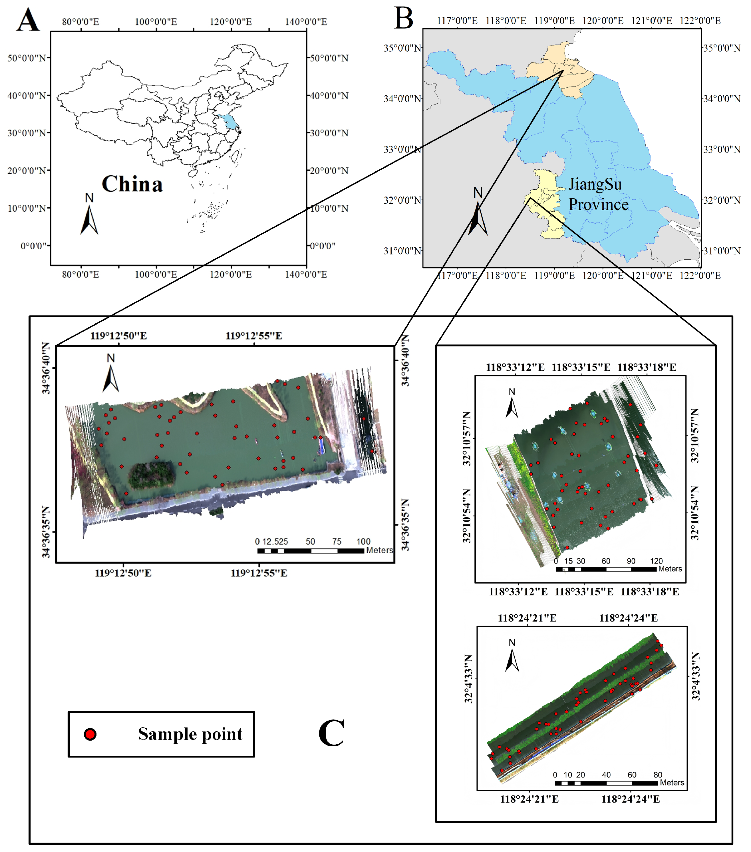
The primary study site is Jingsi Lake, located in Haizhou District, Lianyungang City, Jiangsu Province, China. This freshwater lake holds considerable ecological and environmental importance. As a key regional water body, it supports the hydrological cycle, sustains aquatic ecosystems, and underpins local livelihoods. It also contributes to water supply and regional climate regulation. In recent years, intensified anthropogenic activities have led to water quality deterioration in the lake. Thus, a comprehensive water quality assessment is essential for evaluating ecological health and informing management strategies. To capture spatial variability, the study extended sampling and UAV surveys to two additional water bodies, fish ponds, and crab ponds at the Nanjing Tongwei Aquaculture Base. Along with Jingsi Lake, these sites form the study’s sampling and UAV observation regions, as shown in Figure 1. The inclusion of ecologically diverse waters broadens environmental variability, enabling more in-depth analysis of spatial water quality distributions.

Figure 1.
Overview of the study area and sampling sites. (A) National map of China indicating the location of Jiangsu Province. (B) Regional map showing the locations of Jingsi Lake and the aquaculture base in Jiangsu Province. (C) UAV-based hyperspectral imagery of three sampling sites: Jingsi Lake (top left), fish pond (top right), and crab pond (bottom right). Red circular markers denote the in situ water sampling points (SP1–SP50) used for validating the hyperspectral water quality inversion results. Each site included 50 sampling points arranged via a grid-based strategy. All maps include scale bars (in meters) and north orientation for geospatial reference.
2.2. Research Framework
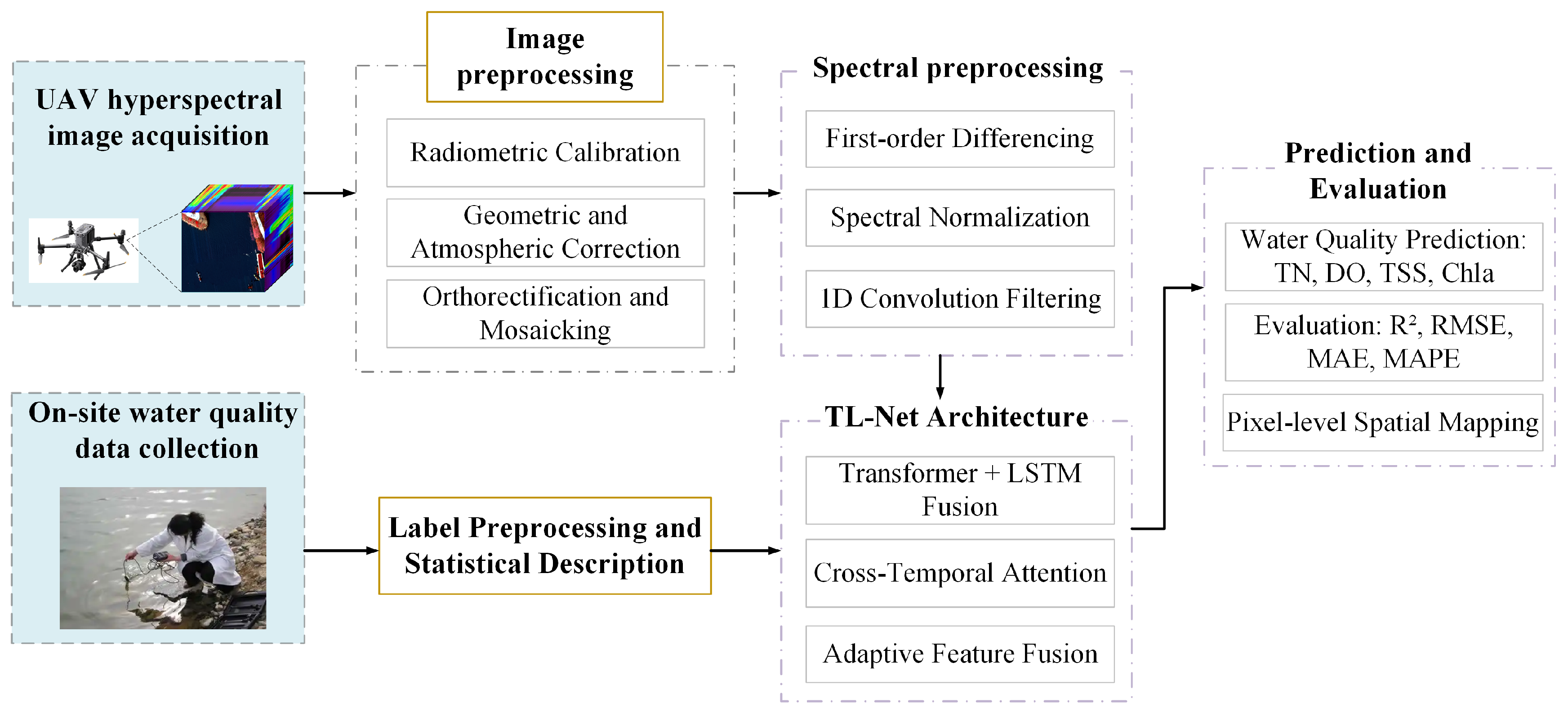
The research framework is shown in Figure 2. Firstly, in Section 2.3, hyperspectral images based on unmanned aerial vehicles were obtained and on-site water quality sampling was carried out. Then, image and label preprocessing are performed in Section 2.3.1 and spectral preprocessing in Section 3.1. The structure of the TL-Net model and the process of feature extraction are detailed in Section 3.2. Subsequently, model training and comparative experiments are conducted in Section 4.4. Finally, the spatial prediction results and accuracy evaluation are presented.
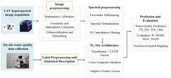
Figure 2.
Research framework.
2.3. Data Acquisition
In this study, experimental data were collected using a quadcopter drone M300 from DJI Innovations and a GaiaSky-mini-Lite developed by Jiangsu Shuanglihe Spectrum Science and Technology Co. Ltd., Wuxi, China to obtain hyperspectral imagery of the study area. The device has a spectral range of 400 to 1000 nm with a spectral resolution of about 3–4 nm and consists of a total of 176 spectral channels. The UAV operates at an altitude of 100 m and captures hyperspectral imaging data with a spatial resolution of about 0.12 m. The GaiaSky-mini-Lite system uses a push-scan imaging mode. The spectrometer has a slit width of only 30 microns and a length of 9.6 mm. When relative motion occurs between the target and the imaging system, a three-dimensional hyperspectral imagery cube is generated.
2.3.1. Data Preprocessing and Labeling
The hyperspectral imagery underwent preprocessing, including lens distortion correction, reflectance calibration, and atmospheric correction, to ensure accurate spectral reflectance. Subsequently, coarse image registration and spatial correction were applied using synchronously acquired visible imagery to enhance spatial consistency. Finally, image mosaicking was performed by integrating POS data, involving alignment, mesh generation, DEM construction, and orthorectification. To support supervised learning, hyperspectral reflectance data were annotated to generate pixel-level labels for TN, DO, TSS, and Chla. These labels were derived from regression models provided by the sensor manufacturer, which correlate reflectance with water quality metrics via validated equations. Despite stable predictions in most cases, edge effects, spectral gaps, and low SNR required further regional optimization. An interpolation-based method combining inverse distance weighting (IDW) and kriging was employed to estimate missing or anomalous pixels. IDW filled gaps using nearby pixels, while kriging leveraged spatial autocorrelation to predict complex spatial variations more accurately.
2.3.2. Field Data Collection
Ground-truth sampling was conducted in three distinct regions (as shown in Figure 1C) to validate the pixel-level water quality labels generated from hyperspectral data and to support the evaluation of deep learning models. Sampling locations were determined using a grid-based strategy. In each region, 50 water samples were collected at a depth of 50 cm below the surface and subsequently analyzed in the laboratory. The ground-truth data were utilized to evaluate the accuracy of water quality labels predicted by the linear regression model and to assess the training effectiveness of deep learning models. Laboratory analyses targeted key water quality parameters: TN, DO, TSS, and Chla. All measurements followed Chinese national standards to ensure data consistency and reliability. The model performance is summarized in Table 1, indicating high accuracy in predicting key water quality parameters. The coefficient of determination (R2) for TN, DO, TSS, and Chla exceeded 0.7, suggesting that the model effectively captured the primary trends. Both the mean squared error (MSE) and root mean squared error (RMSE) values were between 0.2 and 0.3, while the mean absolute percentage error (MAPE) ranged from 10% to 20%, indicating acceptable relative prediction errors. These results demonstrate the reliability of the pixel-level water quality labels generated by the linear regression model.

Table 1.
Water quality parameter curve fitting results.
3. Methods
3.1. Spectral Data Processing and Analysis
3.1.1. Spectral Preprocessing
First-order differencing is a common preprocessing technique in water quality parameter estimation using spectral data. This approach frames the problem as a regression task, with the input being derived from first-order differenced spectral characteristics. It effectively suppresses linear background noise, enhances overlapping spectral feature identification, and improves subtle spectral fluctuation representation. First-order differencing also mitigates surface mirror effects, reducing specular reflection impact on water quality retrieval and improving model robustness. This approach is widely applied in water quality parameter modeling [33].
Although generally effective, the effectiveness of first-order differencing varies among different water quality parameters due to variations in their respective spectral response characteristics. For instance, in our experiments, TN and DO exhibited significant improvements in spectral correlation within the near-infrared region after differencing, indicating an increased sensitivity to subtle spectral variations. TSS demonstrated notable benefits in the visible to near-infrared (NIR) transition range (500–750 nm), where scattering effects are particularly prominent. Chla showed pronounced enhancement in the red-edge region (approximately 710 nm), which aligns with known Chla absorption features. These findings suggest that although first-order differencing is broadly effective across all four parameters, its effectiveness is parameter-specific and is most pronounced when aligned with parameter-specific spectral sensitivity regions. The first-order difference is calculated as follows:
where denotes the wavelength and represents the spectrum derived from first-order differencing at . and represent the spectral reflectance at adjacent wavelengths and , respectively.
3.1.2. Spectral Feature Extraction
In this study, we designed a feature extraction module to extract relevant features from spectral data for subsequent tasks. The module employs one-dimensional convolution to capture local spectral patterns and suppress background noise. This facilitates the differentiation of overlapping spectral features and enhances the signal-to-noise ratio. Specifically, the module applies a convolution kernel to the input spectral data, followed by batch normalization and ReLU activation to enhance feature representation. Adaptive averaging pools ensure that the output feature length remains fixed, independent of input size. This approach efficiently extracts meaningful spectral information, crucial for accurate regression modeling in tasks like water quality parameter estimation. The module operates as follows:
where is the output feature map and is the 1D convolution applied to the input , followed by batch normalization and ReLU activation.
3.1.3. Pearson Correlation Analysis
Covariance is calculated by normalizing the product of two variables to quantify their statistical relationship. This study examined the relationship between surface reflectance and water quality parameters, selecting relevant spectral bands for inversion model construction [34]. The Pearson correlation coefficient was used, derived by normalizing the product of covariance and the standard deviation of the variables, to quantify the correlation between them. The formula is expressed as:
where is the correlation coefficient between surface reflectance and water quality parameters. Specifically, and are the observed values of surface reflectance and water quality parameters, respectively, and and are their mean values. The correlation coefficient ranges from , with values closer to 1 indicating a stronger linear correlation and values near 0 suggesting a weaker correlation.
3.2. Regression Methods
In this study, the linear regression method PLSR is used to compare with six traditional machine learning methods and the proposed TL-Net network [35]. The six traditional machine learning methods are SVR, Xgboost, Catboost, CNN, LSTM, Transformer, and the proposed TLNet networking method. In the following, we introduce the traditional machine learning method model and the parameters and structure of the proposed TL-Net network.
3.2.1. Proposed TL-Net Model
Figure 3 illustrates the architecture of TL-Net, a hybrid deep learning framework designed for water quality parameter retrieval using hyperspectral imagery. TL-Net integrates LSTM and Transformer encoders in a parallel structure to simultaneously capture both global and local spectral dependencies. The overall architecture comprises five major components: spectral feature extraction, a Transformer encoder, an LSTM network, cross-temporal attention, and adaptive fusion. The spectral feature extraction module employs one-dimensional convolution to extract localized spectral features and suppress background noise. The Transformer encoder captures global contextual dependencies across the entire spectral sequence, enabling the model to recognize long-range feature interactions. In contrast, the LSTM network is particularly effective in modeling local sequential relationships, capturing fine-grained temporal dynamics within the spectral data. These two modules are designed to operate in parallel, leveraging their complementary strengths: the Transformer excels at global representation learning, while the LSTM preserves short-range spectral continuity and contextual information. To integrate these complementary features, the cross-temporal attention module facilitates dynamic interaction between the outputs of the Transformer and LSTM branches. Subsequently, the adaptive feature fusion module employs a gating mechanism to perform weighted combination of global and local features, generating the final feature representation for regression. This multi-branch, fusion-driven architecture allows TL-Net to maintain robustness across heterogeneous spectral characteristics and achieve improved generalization performance. By jointly modeling local feature patterns, global contextual dependencies, and their dynamic interactions, TL-Net significantly enhances the accuracy and stability of water quality parameter estimation.
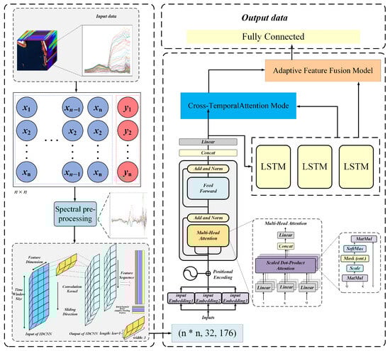
Figure 3.
Overall architecture of the proposed TL-Net framework for multi-parameter water quality inversion using UAV-based hyperspectral imagery. The pipeline starts with hyperspectral image input and spectral preprocessing, including first-order differentiation to enhance informative features. The preprocessed spectral data are transformed into a structured input sequence via a sliding window and fed into two parallel modules: a Transformer encoder, which captures global spectral dependencies using multi-head attention and positional encoding, and an LSTM network, which learns local sequential patterns. The outputs from the two branches are fused through a cross-temporal attention module, which facilitates dynamic interactions between global and local features. An adaptive feature fusion module then assigns weights to integrate the representations, and the fused features are finally passed to a fully connected layer to predict water quality parameters, including TN, DO, TSS, and Chla.
3.2.2. LSTM Model
LSTM, as illustrated in Figure 4, is a specialized recurrent neural network (RNN) architecture commonly employed for time series data processing and is particularly effective in capturing long-term dependencies. LSTM networks have demonstrated strong performance across various time series prediction tasks [36,37,38]. Its core design relies on memory cells regulated by gating mechanisms, enabling the modeling of dynamic behaviors and complex sequences over extended temporal horizons. However, LSTM networks face challenges such as vanishing or exploding gradients when handling ultra-long sequences. Each LSTM unit contains three main gates: forget, input, and output gates, whose operations are defined as follows:
where is the cell state, is the output gate, is the hidden state, is the forget gate, and is the input gate. Specifically, the forget gate determines which information from the previous cell state should be retained or discarded; the input gate regulates how much of the new candidate information is integrated into the current memory; and the output gate controls the exposure of the updated cell state to the next hidden state . The symbol “∘” denotes element-wise (Hadamard) multiplication, while all W terms refer to learnable weight matrices and b terms denote the corresponding bias vectors. These mechanisms collectively enable the LSTM to model and update sequential data with long-range temporal dependencies.
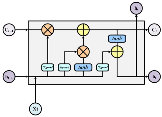
Figure 4.
Structure of an LSTM unit. The cell processes the input , previous hidden state , and cell state through forget, input, and output gates to generate the updated hidden state and cell state , enabling long-term sequence modeling.
3.2.3. Transformer
In time series modeling, recurrent neural networks (RNNs) such as LSTM are widely used but often struggle to capture long-term dependencies in high-dimensional data under complex spectral variations [39,40]. The Transformer architecture addresses this limitation by modeling global dependencies through self-attention, demonstrating superior performance in sequence learning tasks [41]. In TL-Net, each pixel’s spectral vector is treated as a sequence, with each band corresponding to a time step. The Transformer encoder captures contextual relationships among bands. Its fundamental operation is the scaled dot-product attention:
where denote the query, key, and value matrices and denotes the scaling dimension.
To enhance representational capacity, multiple attention heads are computed in parallel:
where each and is a projection matrix. The output is further transformed via a feed-forward network (FFN) with two linear layers:
where and are parameters. Each Transformer encoder block integrates residual connections and layer normalization:
ensuring gradient stability and improved convergence during training.
In TL-Net, Transformer-extracted global spectral features are fed into both the LSTM module and a cross-temporal attention mechanism. This design leverages the Transformer’s ability to capture non-local dependencies and complements the LSTM’s sequential modeling capability. This combination enhances the model’s ability to estimate water quality parameters across ecologically diverse and spatially heterogeneous inland waters.
3.2.4. Cross-Temporal Attention Module
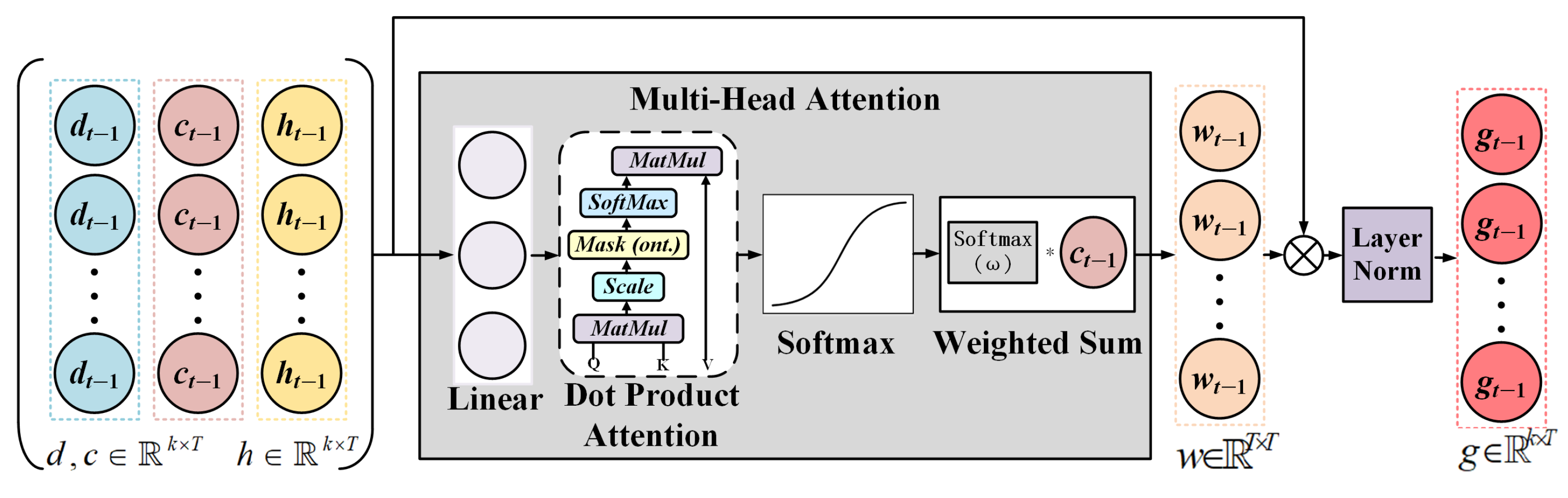
The cross-temporal attention module was designed to fuse local features extracted by the LSTM with global features from the Transformer. The module employs a multi-head attention mechanism to dynamically select relevant global features from the Transformer for the local features provided by the LSTM, generating optimized representations. The module input consists of the Transformer’s outputs, d and c, as key and value, respectively, and the LSTM hidden state, h, as query. Attention weights are obtained by normalizing scores with the softmax function and calculating the dot product similarity between query and key. The weighted output features are calculated by applying these weights to the value:
To preserve original local information, the module introduces a residual connection that adds the attention output to the LSTM hidden state, followed by layer normalization to produce the final optimized features . This design ensures effective combination of local and global features, providing richer representations for subsequent tasks. The overall process is illustrated in Figure 5.
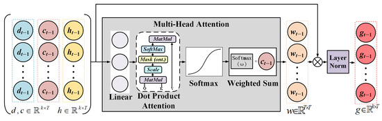
Figure 5.
Illustration of the cross-temporal attention module designed to integrate global and local spectral-temporal features. The Transformer-derived global features () and the LSTM hidden state () are used as key and query, respectively, in a multi-head attention mechanism. The resulting weighted context vector is combined with the original LSTM output () through residual addition and layer normalization, producing the refined representation .
3.2.5. Adaptive Feature Fusion Module
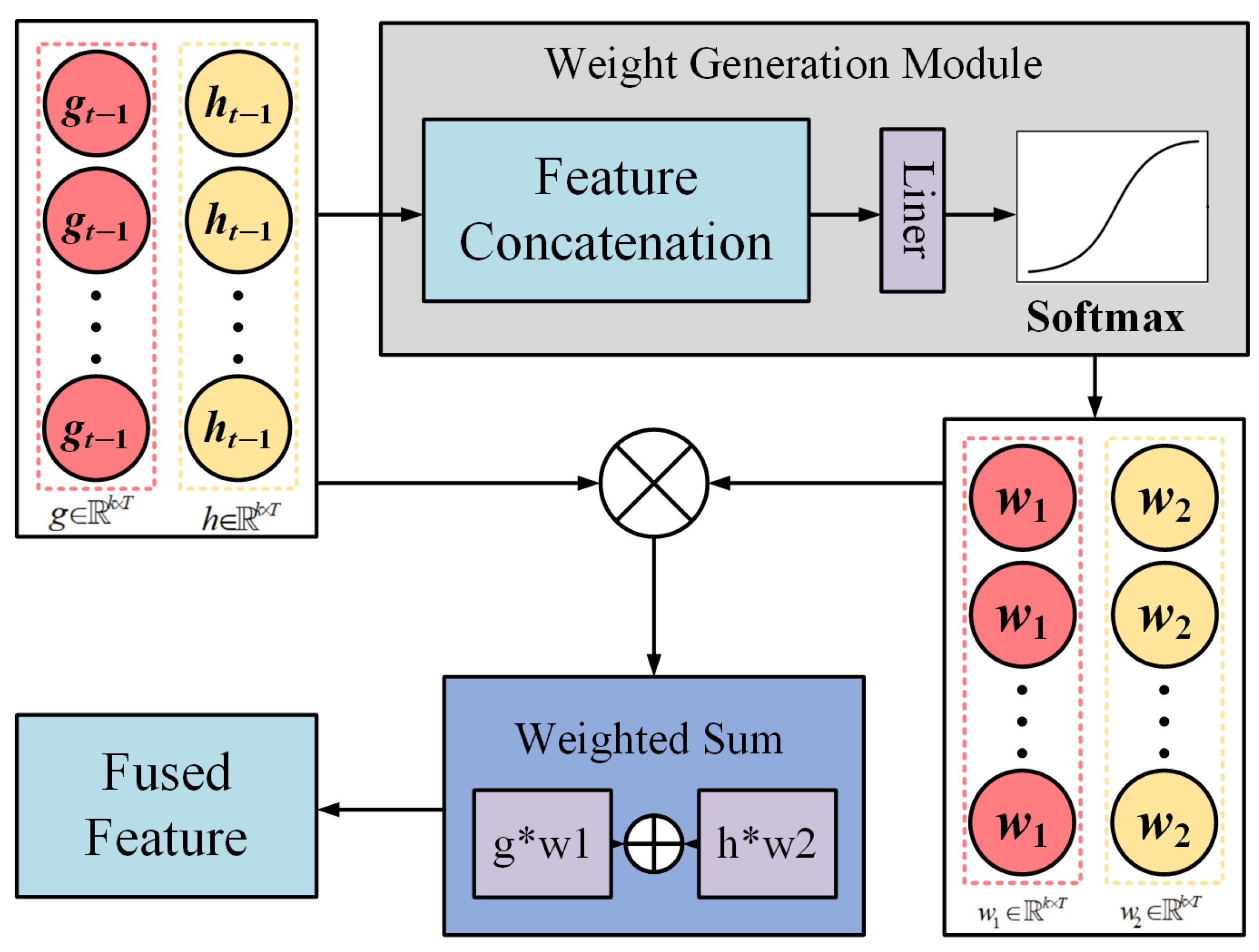
The adaptive fusion module dynamically combines the outputs of the cross-temporal attention mechanism (g) and the LSTM module (h) to produce the final fused feature representation (). As illustrated in Figure 5, g represents the global context feature, which is derived from the interaction between the Transformer encoder’s output and the LSTM’s temporal features through the cross-temporal attention mechanism. On the other hand, h is the raw output of the LSTM, preserving local temporal patterns that may not be fully captured by the attention mechanism. Both g and h are feature matrices with dimensions , where B denotes the batch size and H is the hidden dimension.
The module begins with feature concatenation, combining g and h along their feature dimension to form a unified representation z, which serves as input to the weight generation module. This step is depicted in the feature concatenation block of Figure 5. The concatenated feature z is then passed through a linear layer, which projects it into a weight space, generating unnormalized weight scores. These scores are normalized using a softmax function, producing two adaptive weights, and , that dynamically determine the relative contributions of g and h to the fused representation.
Subsequently, the weights and are applied to g and h, respectively, in the element-wise weighting step. As shown in Figure 6, this operation adjusts each feature’s importance according to the adaptive weights. The weighted features are then summed element-wise in the weighted sum block to produce the final fused feature :
where · denotes element-wise multiplication.
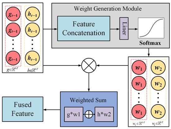
Figure 6.
Structure of the adaptive feature fusion module. It combines the global feature vector from the cross-temporal attention module () and the local feature vector from the LSTM output (). The two features are concatenated and passed through a linear layer and softmax activation to generate adaptive weights. The final fused representation is obtained via weighted summation, enabling dynamic integration of global and local information.
The resulting fused feature, , integrates the global context information from g and the local temporal patterns from h. Adaptive weights and ensure flexibility by dynamically adjusting the contributions of g and h for each sample. This allows the fusion module to adapt to varying input characteristics. The adaptive fusion module leverages three core components, feature concatenation, weight generation module, and weighted sum, to effectively integrate global and local features, yielding a comprehensive representation for subsequent prediction tasks.
3.2.6. Training Settings
To improve the performance of TL-Net on limited hyperspectral training data, we incorporated several optimization techniques tailored for small-sample learning scenarios. Specifically, in the Transformer submodule, dropout layers with a rate of 0.2 were applied after the multi-head attention and feed-forward sub-layers to prevent overfitting. Layer normalization was adopted to stabilize training dynamics and improve convergence. In addition, L2 weight regularization was introduced into the loss function to constrain model complexity and enhance generalization.
The TL-Net model was implemented using the PyTorch (v2.6.0, CUDA 12.4) deep learning framework and trained on an NVIDIA RTX 2060 SUPER GPU. The network was optimized using the Adam optimizer with an initial learning rate of 0.005 and a mini-batch size of 64. Training was performed for 200 epochs, and an early stopping mechanism was applied based on the validation loss, with a patience of 10 epochs to prevent overfitting. A learning rate scheduler was used to reduce the learning rate by a factor of 0.5 when the validation performance plateaued. The loss function adopted for model training was the mean squared error (MSE), consistent with the regression objectives of water quality parameter estimation. Hyperparameters, including the number of Transformer layers, the dimensionality of hidden states in the LSTM module, and the size of the fused feature vectors, were selected through grid search on the validation dataset.
3.3. Model Evaluation
In this study, standard regression assessment metrics, including the coefficient of determination (R2), mean squared error (MSE), root mean squared error (RMSE), mean absolute error (MAE), and mean absolute percentage error (MAPE), were employed to evaluate the model’s performance. These metrics collectively provide a comprehensive evaluation of the model’s predictive accuracy. The following provides the mathematical expressions for each metric:
where is the actual value, is the predicted value, is the mean of the actual values, and n is the number of observations. A model is generally considered to perform well if it exhibits higher values and lower MSE, RMSE, MAE, and MAPE values.
4. Results
4.1. Data Analysis
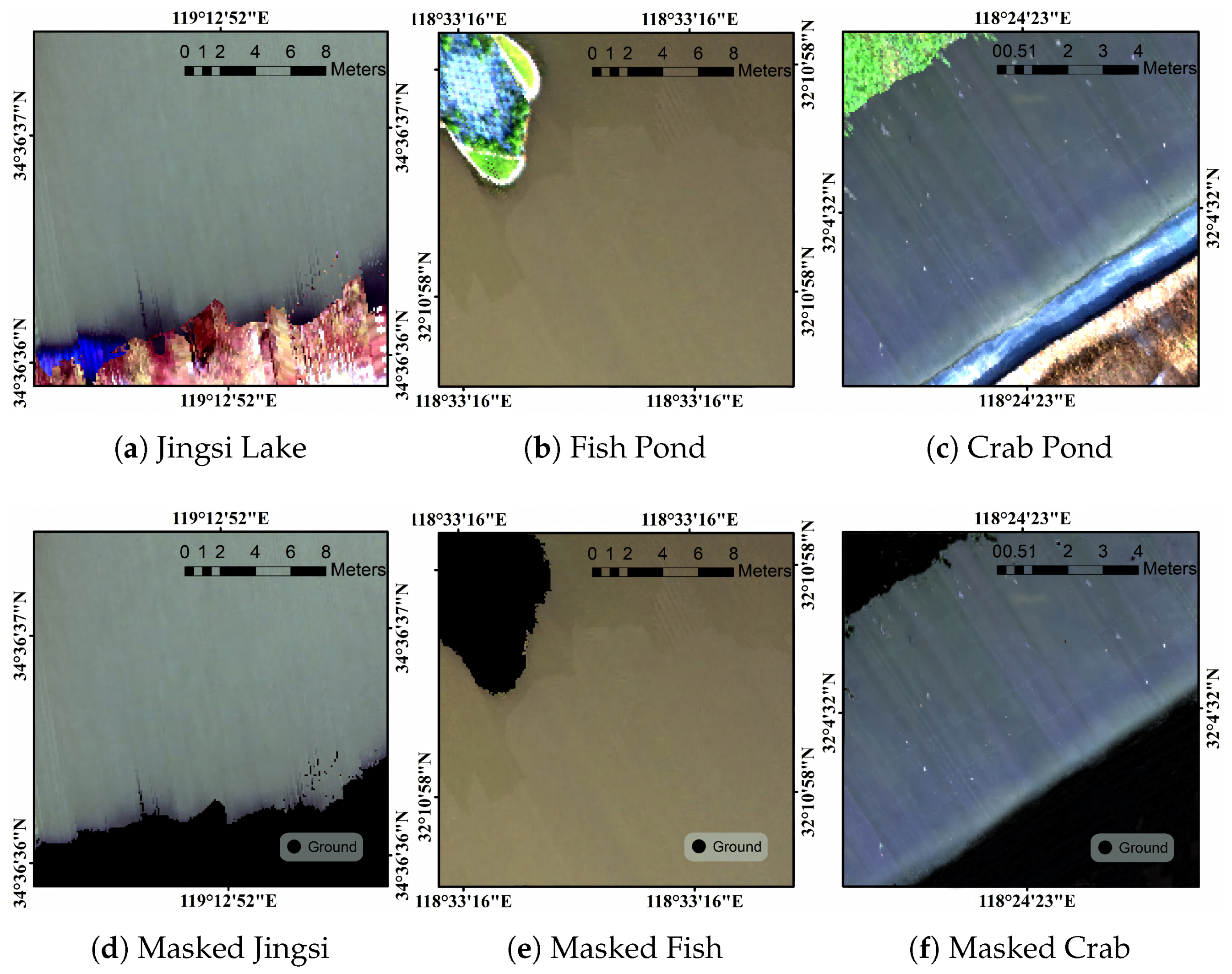
The data for this study were collected from three regions: Jingsi Lake, a fish pond, and a crab pond. Three 200 × 200-pixel subregions were selected from each region as hyperspectral data samples, as shown in Figure 7a–c. A masking method was applied to retain only water regions, removing terrestrial objects such as vegetation, soil, and buildings, ensuring the accuracy of the training data. Water pixels from different regions were then integrated into a unified dataset, balancing samples from each region while accounting for regional water quality differences. This approach maximized sample diversity. Data from Jingsi Lake reflect the stable characteristics of a natural lake, whereas data from the fish and crab ponds show variability due to aquaculture. Integrating these samples enhanced the model’s adaptability to diverse water quality environments.
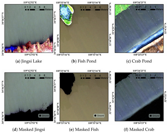
Figure 7.
Local hyperspectral imagery and mask results were obtained for various water quality: (a) Jingsi Lake, Lianyungang, Jiangsu; (b) fish culture pond at Nanjing Tongwei Aquaculture Base; (c) crab rearing pond at Nanjing Tongwei Aquaculture Base; (d) water-only region of Jingsi Lake after masking; (e) water-only region of the fish pond after masking; (f) water-only region of the crab pond after masking.
4.2. Spectral Band Correlation Analysis and Water Quality Parameter Relationships
Figure 8 illustrates the results of hyperspectral imagery preprocessing and correlation analysis. Figure 8a shows the Pearson correlation heatmap of raw spectral bands, highlighting strong correlations in the lower and upper spectral ranges, indicative of spectral redundancy. Figure 8b presents the heatmap after first-order derivative processing, where inter-band correlations are refined, background effects are reduced, and localized variations are enhanced. Figure 8c compares raw and derivative spectra, emphasizing variations across specific wavelengths.
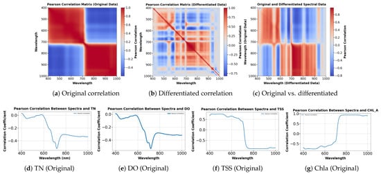
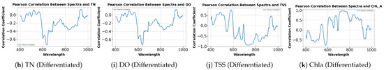
Figure 8.
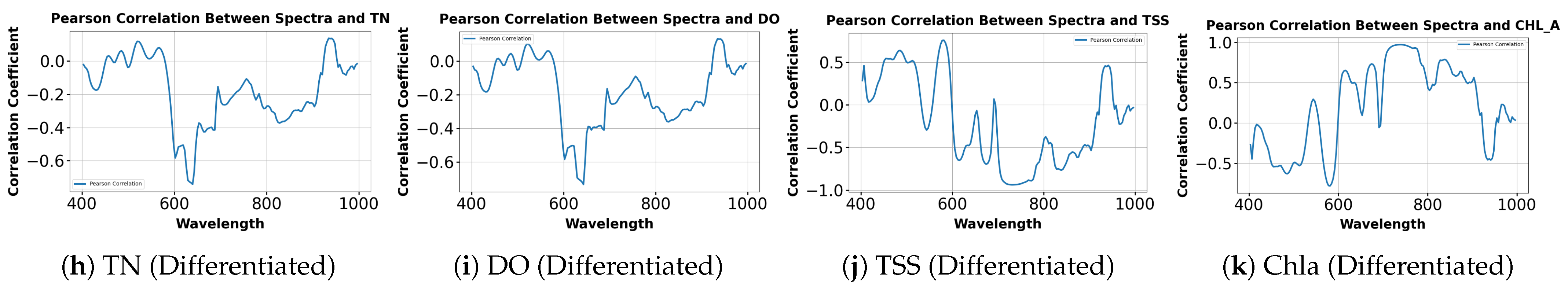
Pearson correlation analysis of spectral data. (a) Correlation matrix of the original spectra. (b) Correlation matrix after first-order differentiation. (c) Comparison of original and differentiated spectra. (d–g) Correlation between original spectra and water quality parameters (TN, DO, TSS, Chla). (h–k) Correlation between differentiated spectra and the same parameters, revealing enhanced feature sensitivity.
Figure 8d through Figure 8k visualize the Pearson correlation coefficients between spectral reflectance (original and differentiated) and water quality parameters (TN, DO, TSS, Chla). These plots reveal distinct correlation trends across wavelengths for each parameter and preprocessing type. Despite the smooth trends in raw spectra, correlation analysis revealed clear associations between hyperspectral reflectance and water quality indicators. For TN and DO, correlation coefficients decreased with wavelength, reaching minima in the short-wave infrared (SWIR) region, indicating notable spectral responses. In contrast, TSS correlations stabilized beyond 700 nm, suggesting that key distinguishing features occur in the visible to near-infrared transition. For Chla, correlations were weak at shorter wavelengths but increased sharply within the red-edge region (700–750 nm), consistent with Chla sensitivity.
First-order derivative processing further enhanced these correlations, revealing sharper spectral features. TN and DO profiles exhibited more fluctuations with multiple local peaks, indicating reduced background interference and amplified spectral responses at sensitive wavelengths. The TSS derivative curve showed distinct fluctuations across 400–900 nm, with local extrema near 500 and 750 nm, highlighting key regions associated with TSS variability. For Chla, derivative processing revealed pronounced fluctuations in the red-edge and near-infrared regions, improving sensitive band identification. Overall, first-order derivative processing clarified spectral correlations, providing a stronger basis for water quality retrieval model development.
4.3. Spectral Differentiation and Convolution Feature Extraction
Hyperspectral imagery contains rich spectral information but is often affected by background noise and low-frequency variations, obscuring subtle differences between samples. Fully exploiting hyperspectral imagery requires a multi-level processing approach, as illustrated in Figure 9. First-order differentiation was first applied to raw reflectance spectra to emphasize local variations, suppress background interference, and improve data separability. A one-dimensional convolutional neural network (1D-CNN) was then applied to the derivative spectra to capture local patterns and extract discriminative deep features. Adaptive pooling was used to integrate and compress the high-dimensional convolutional features. This step reduced dimensionality while preserving key spectral information, enhancing sample separability. This multi-stage approach optimized feature representation across multiple levels. Adaptive pooling further refined the features, constructing a more compact and discriminative feature space. Overall, this strategy significantly improved data separability and provided a robust feature foundation for hyperspectral water quality inversion.
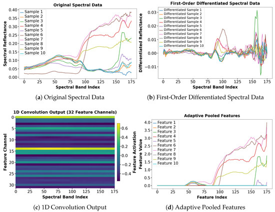
Figure 9.
The visualization of spectral data processing and feature extraction. (a) Original spectral data showing reflectance distributions of different samples, (b) first-order differentiated spectral data highlighting local spectral variations, (c) 1D convolution output representing activations across 32 feature channels, and (d) adaptive pooled features illustrating compressed and integrated spectral characteristics.
4.4. Analysis and Comparison of Water Parameter Estimation Models
The dataset used in this study consists of hyperspectral data collected from three regions, along with the corresponding pixel-level labels for four water quality parameters: TN, DO, TSS, and Chla. The dataset was randomly divided into training and testing sets at a 7:3 ratio, with 70% of the samples used for training and 30% for testing. Eight models, including PLSR, SVR, XGBoost, CatBoost, CNN, LSTM, Transformer, and the proposed TL-Net, were employed for regression analysis of these water quality parameters. The performance of the models is summarized in Table 2, showing that the PLSR model demonstrated the lowest prediction accuracy. Its R2 values for TN and DO predictions were 0.8067 and 0.8068, respectively, with MAPE values of 24.96% and 65.55%, indicating its limited ability to model the complex nonlinear relationships in hyperspectral imagery. This limitation reduces its suitability for pixel-level water quality retrieval. For TSS and Chla, the PLSR model achieved R2 values of 0.8858 and 0.8768, respectively, but the prediction errors were still significant. In contrast, the SVR model exhibited improved regression performance for TN and TSS predictions, with R2 values increasing to 0.9357 and 0.9325, respectively, and the MAPE for TN decreasing to 7.18%. However, the SVR model still struggled with DO and Chla predictions, yielding MAPE values of 18.06% and 7.34%, respectively, highlighting its instability and limited suitability for multi-parameter regression tasks. Machine learning models, such as XGBoost and CatBoost, further improved regression performance. Among these, the CatBoost model achieved notable results for TN and DO predictions, with R2 values of 0.9494 and 0.9566 and RMSE values of 0.1790 and 0.0869, respectively.
Table 2.
Results of regression analysis for water quality indices. Bold values indicate the best performance among all compared models.
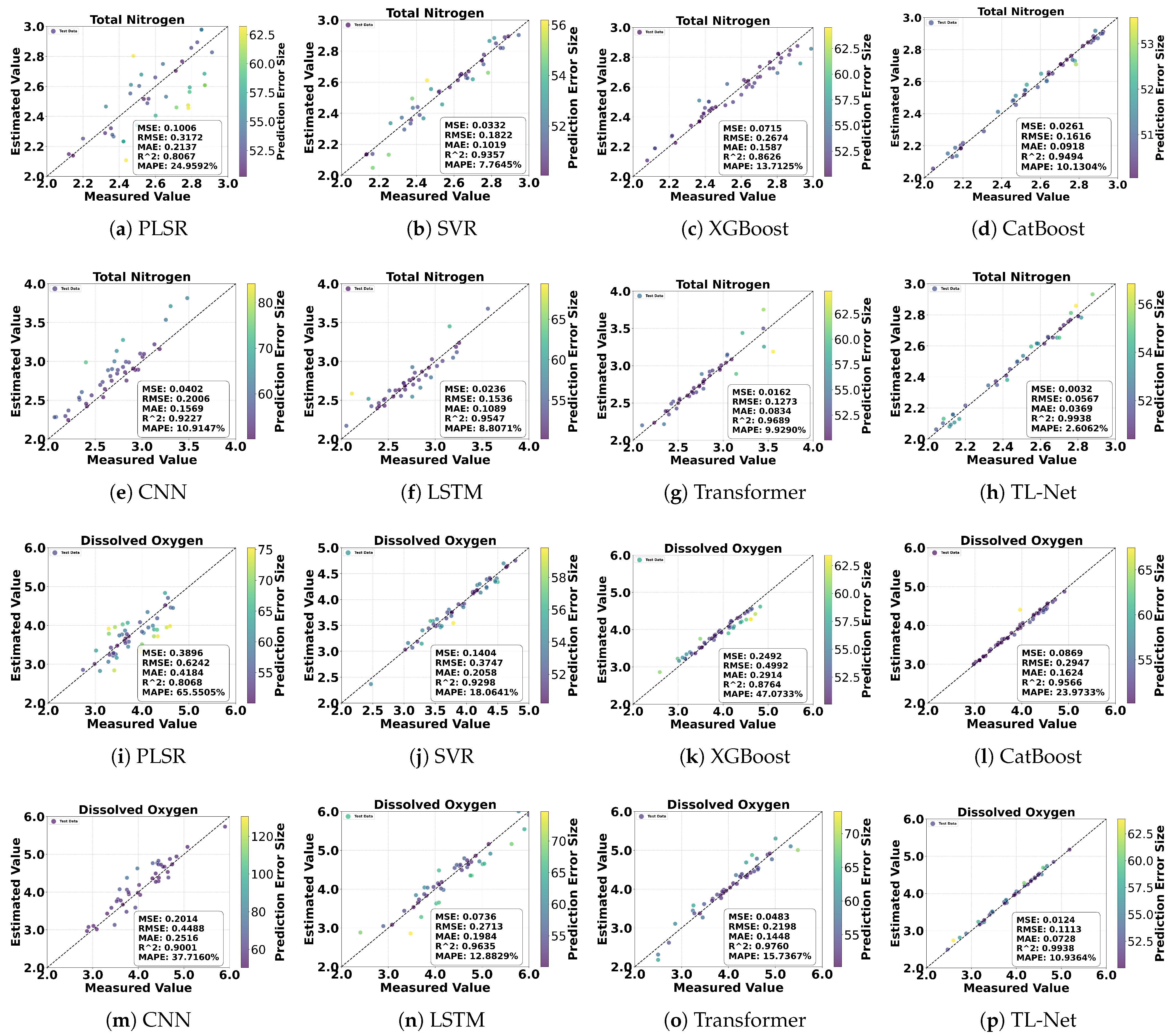
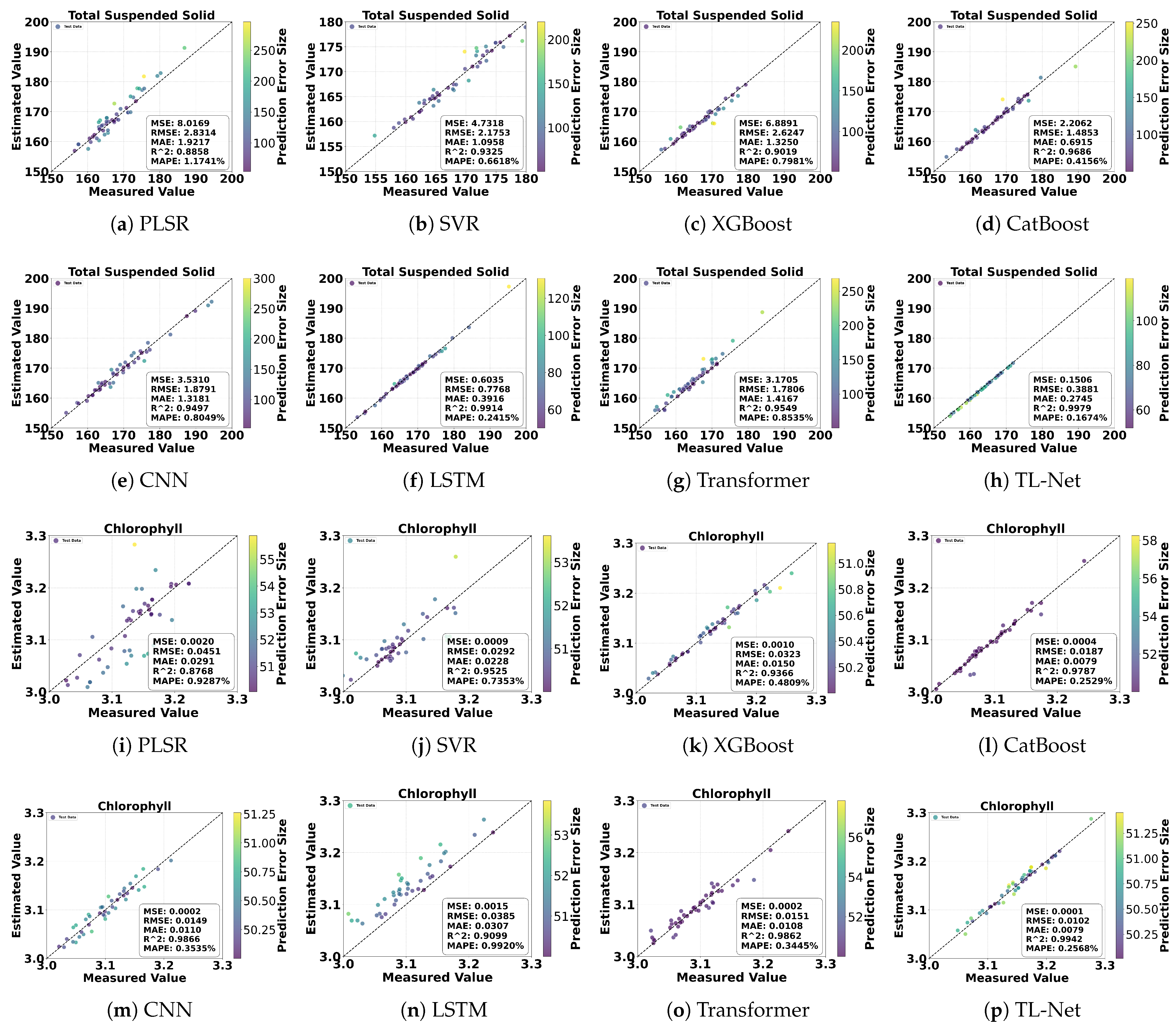
However, despite improvements over traditional methods, these machine learning models fell short of the accuracy achieved by deep learning models. Deep learning models demonstrated substantial advantages across all four parameters. The LSTM model achieved R2 values of 0.9547 and 0.9635 for TN and DO predictions, with MAPE values being reduced to 8.81% and 12.88%, respectively. The Transformer model further improved regression performance, achieving R2 values of 0.9689 and 0.9863 for TN and DO, with RMSE values reduced to 0.1273 and 0.1660. For TSS and Chla, the Transformer model also exhibited excellent performance, with R2 values of 0.9549 and 0.9862, respectively. The proposed TL-Net model outperformed all other models, utilizing pixel-level hyperspectral data as the input. For TN and DO, TL-Net achieved R2 values of 0.9938 and 0.9938, RMSE values of 0.0567 and 0.1113, and MAPE values that were reduced to 2.60% and 10.93%, respectively. For TSS and Chla, TL-Net achieved R2 values of 0.9979 and 0.9942 and MAPE values of only 0.16% and 0.25%, demonstrating its superior regression capabilities. Figure 10 and Figure 11 visually present the regression performance by comparing observed and predicted values. The scatter plots for the PLSR and SVR models show a relatively dispersed distribution, with many points deviating from the 1:1 line. In contrast, the TL-Net model’s scatter points closely align with the 1:1 line, with most points appearing deep blue, indicating minimal prediction errors. Only a few points appear in light yellow, representing minor prediction errors. Particularly for complex parameters like TSS and Chla, the TL-Net model’s regression performance significantly outperformed that of other models.
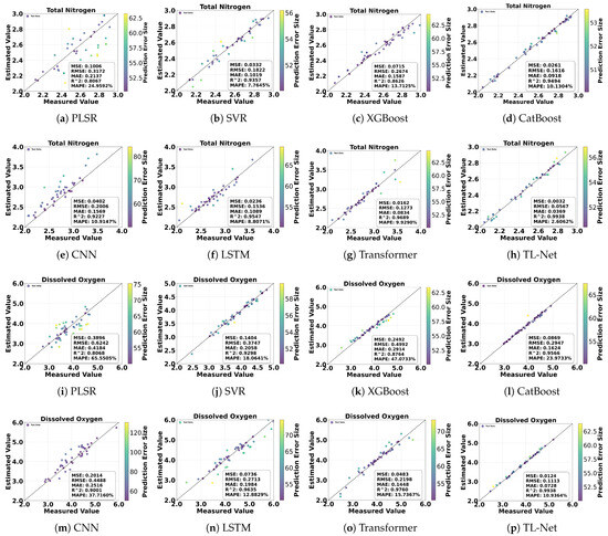
Figure 10.
Comparison of different models for TN and DO prediction: (a,i) PLSR, (b,j) SVR, (c,k) XGBoost, (d,l) CatBoost, (e,m) CNN, (f,n) LSTM, (g,o) Transformer, and (h,p) TL-Net.
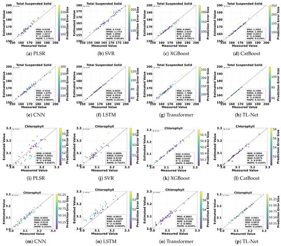
Figure 11.
Comparison of different models for TSS and Chla prediction: (a,i) PLSR, (b,j) SVR, (c,k) XGBoost, (d,l) CatBoost, (e,m) CNN, (f,n) LSTM, (g,o) Transformer, and (h,p) TL-Net.
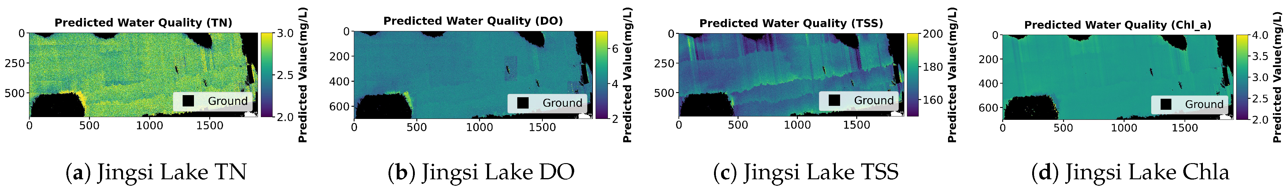
In addition to numerical regression metrics, the spatial distributions of predicted water quality parameters are visualized in Figure 12. These maps illustrate pixel-level estimations of TN, DO, TSS, and Chla across Jingsi Lake, fish ponds, and crab ponds. The predicted distributions highlight regional differences among the three water bodies, with relatively homogeneous patterns being observed in the lake and greater spatial variability being detected in aquaculture environments. These spatial results further demonstrate the capability of the TL-Net model to capture fine-scale variations in water quality using hyperspectral imagery.

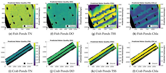
Figure 12.
Visualization of predicted water quality parameters for different aquatic environments: (a–d) predicted TN, DO, TSS, and Chla for Jingsi Lake; (e–h) predicted TN, DO, TSS, and Chla for fish ponds; (i–l) predicted TN, DO, TSS, and Chla for crab ponds.
5. Discussion
In recent years, deep learning has gained significant attention in hyperspectral imagery analysis for water quality assessment. Traditional machine learning models, such as PLSR, SVR, and CatBoost, often struggle to capture the complex, nonlinear relationships between hyperspectral reflectance and water quality parameters, especially in optically heterogeneous and anthropogenically impacted systems. The complexity of HSI data across spatial and spectral dimensions limits the generalizability of conventional models in diverse aquatic environments.
To address these challenges, this study proposes TL-Net, a novel hybrid deep learning framework designed to estimate multiple water quality parameters in ecologically diverse and multi-scale inland water bodies. The architecture integrates Transformer and LSTM modules, augmented by a cross-temporal attention mechanism and an adaptive feature fusion strategy. Experimental results demonstrate that TL-Net consistently outperforms both traditional models and advanced deep learning approaches across four key water quality indicators: TN, DO, TSS, and Chla. Compared with existing baselines, TL-Net achieves significantly higher R2 values (all exceeding 0.99) while notably reducing RMSE and MAPE, indicating its superior performance in high-resolution water quality prediction tasks. The strength of the model lies in its ability to simultaneously capture global dependencies in the spectral domain and local dynamic features within temporal sequences. The Transformer encoder effectively models non-local dependencies across spectral bands, while the LSTM structure excels at capturing contextual information related to local variations. The incorporation of the cross-temporal attention mechanism facilitates efficient information exchange between modules, enhancing the model’s ability to selectively emphasize relevant features. The adaptive feature fusion module further ensures dynamic optimization of the output based on spectral context. Together, these architectural components enhance the model’s robustness and adaptability to highly heterogeneous aquatic environments.
While these results highlight the strong predictive capability of TL-Net, the exceptionally high R2 values (all exceeding 0.99) also raise potential concerns regarding overfitting, particularly given the limited size and diversity of the training dataset. To mitigate this risk, we adopted multiple regularization strategies, including dropout layers (with a rate of 0.2), L2 weight penalties, and early stopping during training. Furthermore, five-fold cross-validation was employed to evaluate model robustness and reduce variance. Despite these measures, we acknowledge the need for further validation using temporally and spatially independent datasets to more rigorously assess the model’s generalization ability in real-world, dynamic aquatic environments.
Spatial prediction results reveal distinct ecological patterns among the three study areas: Jingsi Lake, fish ponds, and crab ponds. TN and TSS concentrations in Jingsi Lake exhibit spatially stable and low-distribution characteristics, reflecting a strong natural self-purification capacity. In contrast, aquaculture ponds show pronounced spatial heterogeneity, with elevated pollutant concentrations near feeding zones and pond margins. These patterns are primarily driven by feed inputs, sediment disturbance, and localized nutrient accumulation. These findings suggest that TL-Net not only excels in predictive accuracy but also provides insights into the ecological mechanisms underlying spatial variations in water quality. The model’s pixel-level prediction capability offers significant potential for real-time, spatially explicit water quality monitoring and management. In aquaculture systems, TL-Net can support decision-making for optimizing feeding strategies and developing waste management plans by identifying pollution hotspots. In natural lakes and riverine systems, the model may be utilized for early detection of diffuse pollution sources and long-term ecological monitoring. Its integration with UAV-based remote sensing platforms enhances operational flexibility and enables rapid deployment across diverse hydrological and geographical settings.
Nevertheless, several limitations remain. First, the current analysis is based on a single sampling campaign, which may constrain the model’s generalizability under seasonal or long-term hydrological variations. Additionally, the model was trained and tested using data from a limited set of spatial locations with relatively similar environmental conditions. This lack of spatial and temporal diversity may hinder the model’s ability to generalize to unseen scenarios or differing water quality regimes. To address this, future work will involve multi-seasonal and multi-location sampling campaigns, incorporating UAV-based hyperspectral data under varied environmental conditions and sensor-viewing geometries to evaluate model robustness. We also plan to test the model on independent water bodies with different ecological and hydrological characteristics to more comprehensively assess its transferability and generalization capacity. Second, the model does not yet incorporate auxiliary ecological variables such as flow velocity, turbidity, and biological indicators, which are critical for improving both predictive accuracy and ecological interpretability. Third, although UAV-based hyperspectral imaging offers high spatial resolution, its applicability is still limited by cost and temporal constraints, potentially hindering large-scale or continuous monitoring efforts.
Furthermore, the current study does not explicitly quantify uncertainty in model predictions. Given the complexity of UAV-based hyperspectral systems and the potential sources of error, including sensor noise, preprocessing artifacts, water sampling inconsistencies, and label estimation inaccuracies, future work will incorporate uncertainty analysis to improve interpretability and risk awareness in practical applications. Techniques such as Monte Carlo dropout, Bayesian deep learning, and ensemble learning frameworks may be integrated to estimate prediction confidence intervals and analyze the propagation of uncertainty through the modeling process. Such approaches are essential for supporting robust decision-making in environmental monitoring and management contexts.
In conclusion, this study presents an end-to-end deep learning framework that effectively integrates Transformer-based spectral feature extraction with LSTM-driven temporal memory mechanisms and adaptive fusion strategies, advancing the methodological development of remote sensing-based water quality assessment. TL-Net provides an accurate, scalable, and ecologically interpretable deep learning solution for aquatic environmental monitoring.
6. Conclusions
This study highlights the significant potential of integrating drone-based hyperspectral imagery with advanced deep learning techniques for monitoring water quality across various aquatic environments. The proposed TL-Net model combines Transformer and LSTM architectures and introduces a cross-temporal attention mechanism and an adaptive feature fusion module, effectively integrating local feature extraction, global dependency modeling, temporal information processing, and multi-scale feature fusion. The model demonstrated exceptional accuracy in estimating both optically active and inactive water quality parameters, including Chla, TSS, TN, and DO. Applying this framework to multi-scale scenarios, such as Jingsi Lake, fish ponds, and crab ponds, provides valuable insights into the spatial heterogeneity of water quality. Quantitative evaluations showed that TL-Net achieved a coefficient of determination (R2) of 0.9938 for TN, a mean absolute error (MAE) of 0.0728 for DO, a root mean square error (RMSE) of 0.3881 for TSS, and a mean absolute percentage error (MAPE) of 0.2568% for Chla, significantly outperforming conventional models in terms of accuracy and robustness. Jingsi Lake, characterized by spatially homogeneous water quality, serves as a baseline for natural systems, while localized pollution near inflow zones underscores the impact of agricultural runoff. In contrast, farmed ponds exhibit significant spatial variability, particularly near feeding and sedimentation zones, emphasizing the direct influence of farming activities on water quality. These findings emphasize the adaptability and robustness of the TL-Net framework in addressing the challenges of monitoring ecologically diverse water bodies. The integration of high-resolution spatial analysis and multi-parameter estimation provides a comprehensive approach for identifying pollution sources and quantifying the impact of human activities. This method lays the foundation for accurate and scalable environmental management techniques, advancing the field of water quality monitoring. Future research could focus on extending TL-Net’s applicability to multi-temporal datasets, enabling dynamic monitoring across seasonal and hydrological cycles. Integrating multi-source data, including satellite imagery and in situ observations may further enhance the model’s generalization and large-scale transferability. In addition, incorporating ecological indicators such as turbidity, phytoplankton diversity, and nutrient flux could improve the interpretability and ecological relevance of the results. These extensions will support real-time environmental protection efforts, intelligent decision support systems, and sustainable aquaculture management.
Author Contributions
Conceptualization, H.L.; methodology, H.L. and N.W.; software, N.W.; validation, D.H., M.S. and Z.Z.; formal analysis, D.H. and D.Y.; data curation, N.W. and Z.D.; original draft writing, H.L.; review and editing, N.W.; supervision, H.L.; project coordination, H.L.; funding acquisition and resources, Z.Z. All authors have read and agreed to the published version of the manuscript.
Funding
This research was funded by the Special Fund for Science and Technology Plan of Jiangsu Province, grant number BE2022385; the National Natural Science Foundation of China, grant number 72174079; the Key Research and Development Plan of Lianyungang City, grant numbers CG2323 and CG2436; and the Excellent Teaching Team of Qinglan Project in Jiangsu Province, grant number 2022-29.
Data Availability Statement
The data presented in this study are available on request from the corresponding author due to the privacy of the data sources.
Conflicts of Interest
The authors declare no conflicts of interest.
References
- Ding, B.; Zhang, J.; Zheng, P.; Li, Z.; Wang, Y.; Jia, G.; Yu, X. Water security assessment for effective water resource management based on multi-temporal blue and green water footprints. J. Hydrol. 2024, 632, 130761. [Google Scholar] [CrossRef]
- Chen, W.; He, B.; Nover, D.; Lu, H.; Liu, J.; Sun, W.; Chen, W. Farm ponds in southern China: Challenges and solutions for conserving a neglected wetland ecosystem. Sci. Total Environ. 2019, 659, 1322–1334. [Google Scholar] [CrossRef] [PubMed]
- Li, H.; Zhao, H.; Wei, C.; Cao, M.; Zhang, J.; Zhang, H.; Yuan, D. Assessing water quality environmental grades using hyperspectral images and a deep learning model: A case study in Jiangsu, China. Ecol. Inform. 2024, 84, 102854. [Google Scholar] [CrossRef]
- Sagan, V.; Peterson, K.T.; Maimaitijiang, M.; Sidike, P.; Sloan, J.; Greeling, B.A.; Maalouf, S.; Adams, C. Monitoring inland water quality using remote sensing: Potential and limitations of spectral indices, bio-optical simulations, machine learning, and cloud computing. Earth-Sci. Rev. 2020, 205, 103187. [Google Scholar] [CrossRef]
- Yang, H.; Kong, J.; Hu, H.; Du, Y.; Gao, M.; Chen, F. A Review of Remote Sensing for Water Quality Retrieval: Progress and Challenges. Remote Sens. 2022, 14, 1770. [Google Scholar] [CrossRef]
- Liu, H.; Li, Z.; Shang, F.; Liu, Y.; Wan, L.; Feng, W.; Timofte, R. Arbitrary-scale Super-resolution via Deep Learning: A Comprehensive Survey. Inf. Fusion 2024, 102, 102015. [Google Scholar] [CrossRef]
- Chen, B.; Mu, X.; Chen, P.; Wang, B.; Choi, J.; Park, H.; Xu, S.; Wu, Y.; Yang, H. Machine learning-based inversion of water quality parameters in typical reach of the urban river by UAV multispectral data. Ecol. Indic. 2021, 133, 108434. [Google Scholar] [CrossRef]
- Liu, X.; Wang, Y.; Chen, T.; Gu, X.; Zhang, L.; Li, X.; Tang, R.; He, Y.; Chen, G.; Zhang, B. Monitoring water quality parameters of freshwater aquaculture ponds using UAV-based multispectral images. Ecol. Indic. 2024, 167, 112644. [Google Scholar] [CrossRef]
- Ding, C.; Pu, F.; Li, C.; Xu, X.; Zou, T.; Li, X. Combining Artificial Neural Networks with Causal Inference for Total Phosphorus Concentration Estimation and Sensitive Spectral Bands Exploration Using MODIS. Water 2020, 12, 2372. [Google Scholar] [CrossRef]
- Chen, J.; Chen, S.; Fu, R.; Li, D.; Jiang, H.; Wang, C.; Peng, Y.; Jia, K.; Hicks, B.J. Remote Sensing Big Data for Water Environment Monitoring: Current Status, Challenges, and Future Prospects. Earth’s Future 2022, 10, e2021EF002289. [Google Scholar] [CrossRef]
- Li, F.; Yigitcanlar, T.; Nepal, M.; Nguyen, K.; Dur, F. Machine learning and remote sensing integration for leveraging urban sustainability: A review and framework. Sustain. Cities Soc. 2023, 96, 104653. [Google Scholar] [CrossRef]
- Guimarães, T.T.; Veronez, M.R.; Koste, E.C.; Souza, E.M.; Brum, D.; Gonzaga, L.; Mauad, F.F. Evaluation of Regression Analysis and Neural Networks to Predict Total Suspended Solids in Water Bodies from Unmanned Aerial Vehicle Images. Sustainability 2019, 11, 2580. [Google Scholar] [CrossRef]
- Niu, Y.; Zhang, L.; Zhang, H.; Han, W.; Peng, X. Estimating Above-Ground Biomass of Maize Using Features Derived from UAV-Based RGB Imagery. Remote Sens. 2019, 11, 1261. [Google Scholar] [CrossRef]
- Shao, Z.; Fu, H.; Li, D.; Altan, O.; Cheng, T. Remote sensing monitoring of multi-scale watersheds impermeability for urban hydrological evaluation. Remote Sens. Environ. 2019, 232, 111338. [Google Scholar] [CrossRef]
- Zhou, Y.; Li, W.; Cao, X.; He, B.; Feng, Q.; Yang, F.; Liu, H.; Kutser, T.; Xu, M.; Xiao, F.; et al. Spatial-temporal distribution of labeled set bias remote sensing estimation: An implication for supervised machine learning in water quality monitoring. Int. J. Appl. Earth Obs. Geoinf. 2024, 131, 103959. [Google Scholar] [CrossRef]
- Lu, X.; Fan, Y.; Hu, Y.; Zhang, H.; Wei, Y.; Yan, Z. Spatial distribution characteristics and source analysis of shallow groundwater pollution in typical areas of Yangtze River Delta. Sci. Total Environ. 2024, 906, 167369. [Google Scholar] [CrossRef]
- Li, H.; Wei, C.; Yang, Y.; Zhong, Z.; Xu, M.; Yuan, D. Unified Dynamic Dictionary and Projection Optimization with Full-Rank Representation for Hyperspectral Anomaly Detection. IEEE J. Sel.Topics Appl. Earth Observ. Remote Sens. 2025, 18, 4032–4049. [Google Scholar] [CrossRef]
- Ali, A.; Zhou, G.; Lopez, F.P.A.; Xu, C.; Jing, G.; Tan, Y. Deep learning for water quality multivariate assessment in inland water across China. Int. J. Appl. Earth Obs. Geoinf. 2024, 133, 104078. [Google Scholar] [CrossRef]
- Mohsen, A.; Ali, Y.; Al-Sorori, W.; Maqtary, N.A.; Al-Fuhaidi, B.; Altabeeb, A.M. A performance comparison of machine learning classifiers for COVID-19 Arabic Quarantine tweets sentiment analysis. In Proceedings of the 1st International Conference on Emerging Smart Technologies and Applications (eSmarTA), Sana’a, Yemen, 10–12 August 2021; pp. 1–8. [Google Scholar]
- Yoosefzadeh-Najafabadi, M.; Earl, H.J.; Tulpan, D.; Sulik, J.; Eskandari, M. Application of Machine Learning Algorithms in Plant Breeding: Predicting Yield from Hyperspectral Reflectance in Soybean. Front. Plant Sci. 2021, 11, 624273. [Google Scholar] [CrossRef]
- Adjovu, G.E.; Stephen, H.; James, D.; Ahmad, S. Overview of the Application of Remote Sensing in Effective Monitoring of Water Quality Parameters. Remote Sens. 2023, 15, 1938. [Google Scholar] [CrossRef]
- Kravitz, J.; Matthews, M.; Bernard, S.; Griffith, D. Application of Sentinel 3 OLCI for chl-a retrieval over small inland water targets: Successes and challenges. Remote Sens. Environ. 2020, 237, 111562. [Google Scholar] [CrossRef]
- Mamun, M.; Kim, J.-J.; Alam, M.A.; An, K.-G. Prediction of Algal Chlorophyll-a and Water Clarity in Monsoon-Region Reservoir Using Machine Learning Approaches. Water 2019, 12, 30. [Google Scholar] [CrossRef]
- Yajima, H.; Derot, J. Application of the Random Forest model for chlorophyll-a forecasts in fresh and brackish water bodies in Japan, using multivariate long-term databases. J. Hydroinform. 2017, 20, 206–220. [Google Scholar] [CrossRef]
- Chen, S.; Fang, G.; Huang, X.; Zhang, Y. Water quality prediction model of a water diversion project based on the improved artificial bee colony–backpropagation neural network. Water 2018, 10, 806. [Google Scholar] [CrossRef]
- Hafeez, S.; Wong, M.S.; Ho, H.C.; Nazeer, M.; Nichol, J.; Abbas, S.; Tang, D.; Lee, K.H.; Pun, L. Comparison of Machine Learning Algorithms for Retrieval of Water Quality Indicators in Case-II Waters: A Case Study of Hong Kong. Remote Sens. 2019, 11, 617. [Google Scholar] [CrossRef]
- Wang, X.; Tan, K.; Du, Q.; Chen, Y.; Du, P. Caps-TripleGAN: GAN-Assisted CapsNet for Hyperspectral Image Classification. IEEE Trans. Geosci. Remote Sens. 2019, 57, 7232–7245. [Google Scholar] [CrossRef]
- Borsoi, R.A.; Imbiriba, T.; Bermudez, J.C.M. Deep Generative Endmember Modeling: An Application to Unsupervised Spectral Unmixing. IEEE Trans. Comput. Imaging 2020, 6, 374–384. [Google Scholar] [CrossRef]
- Zhan, L.; Xu, Y.; Zhu, J.; Liu, Z. Optimizing Chlorophyll-a Concentration Inversion in Coastal Waters Using SVD and Deep Learning Approach. IEEE J. Sel. Top. Appl. Earth Obs. Remote Sens. 2025, 18, 907–920. [Google Scholar] [CrossRef]
- Gong, Z.; Zhong, P.; Yu, Y.; Hu, W.; Li, S. A CNN with Multiscale Convolution and Diversified Metric for Hyperspectral Image Classification. IEEE Trans. Geosci. Remote Sens. 2019, 57, 3599–3618. [Google Scholar] [CrossRef]
- Ullah, F.; Ullah, I.; Khan, R.U.; Khan, S.; Khan, K.; Pau, G. Conventional to Deep Ensemble Methods for Hyperspectral Image Classification: A Comprehensive Survey. IEEE J. Sel. Top. Appl. Earth Obs. Remote Sens. 2024, 17, 3878–3916. [Google Scholar] [CrossRef]
- Pyo, J.; Duan, H.; Baek, S.; Kim, M.S.; Jeon, T.; Kwon, Y.S.; Lee, H.; Cho, K.H. A convolutional neural network regression for quantifying cyanobacteria using hyperspectral imagery. Remote Sens. Environ. 2019, 233, 111350. [Google Scholar] [CrossRef]
- Niu, C.; Tan, K.; Jia, X.; Wang, X. Deep learning based regression for optically inactive inland water quality parameter estimation using airborne hyperspectral imagery. Environ. Pollut. 2021, 286, 117534. [Google Scholar] [CrossRef] [PubMed]
- Cao, X.; Zhang, J.; Meng, H.; Lai, Y.; Xu, M. Remote sensing inversion of water quality parameters in the Yellow River Delta. Ecol. Indic. 2023, 155, 110914. [Google Scholar] [CrossRef]
- Meacham-Hensold, K.; Montes, C.M.; Wu, J.; Guan, K.; Fu, P.; Ainsworth, E.A.; Pederson, T.; Moore, C.E.; Brown, K.L.; Raines, C.; et al. High-throughput field phenotyping using hyperspectral reflectance and partial least squares regression (PLSR) reveals genetic modifications to photosynthetic capacity. Remote Sens. Environ. 2019, 231, 111176. [Google Scholar] [CrossRef]
- Cai, J.; Meng, L.; Liu, H.; Chen, J.; Xing, Q. Estimating Chemical Oxygen Demand in estuarine urban rivers using unmanned aerial vehicle hyperspectral images. Ecol. Indic. 2022, 139, 108936. [Google Scholar] [CrossRef]
- Guo, Q.; Fang, L.; Wang, R.; Zhang, C. Multivariate Time Series Forecasting Using Multiscale Recurrent Networks with Scale Attention and Cross-Scale Guidance. IEEE Trans. Neural Netw. Learn. Syst. 2025, 36, 540–554. [Google Scholar] [CrossRef]
- Huang, R.; Wei, C.; Wang, B.; Yang, J.; Xu, X.; Wu, S.; Huang, S. Well performance prediction based on Long Short-Term Memory (LSTM) neural network. J. Petrol. Sci. Eng. 2022, 208, 109686. [Google Scholar] [CrossRef]
- Ray, P.; Reddy, S.S.; Banerjee, T. Various dimension reduction techniques for high dimensional data analysis: A review. Artif. Intell. Rev. 2021, 54, 3473–3515. [Google Scholar] [CrossRef]
- Zhou, H.; Zhang, S.; Peng, J.; Zhang, S.; Li, J.; Xiong, H.; Zhang, W. Informer: Beyond efficient transformer for long sequence time-series forecasting. Proc. AAAI Conf. Artif. Intell. 2021, 35, 11106–11115. [Google Scholar] [CrossRef]
- Ansar, W.; Goswami, S.; Chakrabarti, A.; Chakroborty, B. A novel selective learning based transformer encoder architecture with enhanced word representation. Appl. Intell. 2022, 53, 9424–9443. [Google Scholar] [CrossRef]


Disclaimer/Publisher’s Note: The statements, opinions and data contained in all publications are solely those of the individual author(s) and contributor(s) and not of MDPI and/or the editor(s). MDPI and/or the editor(s) disclaim responsibility for any injury to people or property resulting from any ideas, methods, instructions or products referred to in the content. |
© 2025 by the authors. Licensee MDPI, Basel, Switzerland. This article is an open access article distributed under the terms and conditions of the Creative Commons Attribution (CC BY) license (https://creativecommons.org/licenses/by/4.0/).