Abstract
The Yellow River Basin (YRB) is a critical ecological zone in China now confronting growing tensions between land conservation and development. This study combines land use, climate, and socio-economic data with spatial–statistical models (GeoDetector [GD]–Patch-generating Land Use Simulation [PLUS]–Integrated Valuation of Ecosystem Services and Trade-Offs [InVEST]) to analyze land use changes (2000–2020), evaluate habitat quality, and simulate scenarios to 2040. Key results include the following: (1) Farmland was decreased by the conversion to forests (+3475 km2) and grasslands (+4522 km2), while construction land expanded rapidly (+11,166 km2); (2) the population and Gross Domestic Product (GDP) pressures drove the farmland loss (q = 0.148 for population, q = 0.129 for GDP), while synergies between evapotranspiration (ET) and the Normalized Difference Vegetation Index (NDVI) promoted forest/grassland recovery (q = 0.155); and (3) ecological protection scenarios increased the grassland area by 12.94% but restricted the construction land growth (−13.84%), with persistent unused land (>3.61% in Inner Mongolia) indicating arid-zone risks. The Habitat Quality-Autocorrelated Coupling Index (HQACI) declined from 0.373 (2020) to 0.345–0.349 (2040), which was linked to drought, groundwater loss, and urban expansion. Proposed strategies including riparian corridor protection, adaptive urban zoning, and gradient-based restoration aim to balance ecological and developmental needs, supporting spatial planning and enhancing the basin-wide habitat quality.
1. Introduction
Land use change studies are critical to understanding the interactions between human activities and the natural environment and have a profound impact on ecological functions caused by the regional climate, soil, and water quality [1,2]. In recent years, rapid urbanization and industrialization have caused the shrinkage of farmland, grassland degradation, soil erosion, and other problems have intensified [3,4]. The Sixth Assessment Report of the IPCC (AR6) indicates clearly that land use change contributes 23% of global anthropogenic GHG emissions. At the same time, land use change directly regulates the energy balance of the regional climate system by altering surface albedo and vegetation evapotranspiration [1,5,6,7]. Analyzing the spatiotemporal evolution patterns of Land Use and Land Cover Change (LUCC) and its multi-scale driving mechanisms has become a scientific prerequisite for coordinating ecological protection and high-quality development [4,8,9].
In recent years, LUCC studies have revealed significant spatiotemporal variability through multi-source data integration [10,11,12], and the spatiotemporal variability of the global LUCC has gradually become apparent in data integration and model simulations. For example, the use of Google Earth Engine monitoring identified deforestation and afforestation as dominant processes in river basin transformations [13], while quantitative assessments demonstrated declining ecosystem service values associated with natural forest loss [14]. Scenario projections highlight complex climate–policy interactions, with large-scale revegetation initiatives showing stronger vegetation recovery than precipitation-driven changes [15] and high-resolution modeling indicating that stringent mitigation policies may strain land systems despite climate warming enabling localized ecological restoration [16]. Globally, LUCC has reshaped 32% of terrestrial areas over six decades, underscoring land use optimization as a critical pathway toward achieving SDGs [17].
Research on land use change, through the application of remote sensing and geographic information system (GIS) technologies, has revealed the dual driving mechanisms of natural processes and human activities at both global and regional scales. Research in this field can elucidate the feedback mechanisms between human activities and ecosystems [18,19,20], providing a scientific reference for regional ecological restoration and policy formulation. The research on the driving mechanisms of land use change has progressively evolved from single-factor analyses to multidimensional interaction studies [21,22,23,24]. Recent methodological advances have enhanced the understanding of LUCC drivers; for example the use of system dynamics modeling identified grassland conservation, water resource management, and environmental investments as critical for balancing ecosystem services with human well-being [25], while coupled Standardized Precipitation–Evapotranspiration Index–Normalized Difference Vegetation Index (SPEI-NDVI) analyses revealed nonlinear farmland degradation responses to extreme droughts, mitigated partially by irrigation infrastructure [26]. These approaches overcome limitations of traditional linear models that inadequately capture complex interactions among isolated factors like precipitation and temperature [12,17].
However, the research has shown that there are nonlinear synergistic effects between climate factors and human activities in the YRB and that the interactive contributions of the factors need to be revealed through the geographical detectors [8,14,27]. Multi-source data integration and model simulations indicated that the northern and southern hemispheres exhibited divergent vegetation dynamics: afforestation and restoration dominated in the northern hemisphere, while natural forest degradation in the southern hemisphere was exacerbated by agricultural expansion [6,7]. The research confirmed that the interaction between climate change and policy regulation significantly reshaped the surface coverage pattern [24,28]. For example, the strong driving force for the ecological restoration of the farmland reforestation project outweighed the effect of precipitation. Among the socio-economic factors, urbanization and population growth were considered the core drivers, and Chen et al. [21] showed that grassland and cropland intertransverse significantly from 2000 to 2020, and future scenario simulations showed that cropland protection policies would inhibit the encroachment of urbanization on cropland and shift to a grassland conversion. Land use change was driven by a combination of factors, including natural conditions, socio-economic dynamics, and policy interventions [12,29]. Scenario modeling is an important tool for predicting future trends of land use change [30,31]. The simulation of future scenarios demonstrated that high-intensity emission reduction policies may put pressure on the land system, but climate warming may create new opportunities for regional ecological restoration, highlighting the need for multi-scale dynamic equilibrium studies.
In the study of habitat quality, recent research has increasingly emphasized habitat quality assessment as a critical tool for evaluating ecological resilience and human–nature interactions in the YRB. The Integrated Valuation of Ecosystem Services and Trade-Offs model has emerged as a widely adopted framework for quantifying habitat quality dynamics, leveraging its capacity to integrate LUCC data with spatial heterogeneity in threat factors and ecosystem sensitivity [32]. For instance, the analyses of the upper and middle YRB revealed divergent trends: while certain regions exhibited a slight decline in habitat quality indices due to agricultural expansion and urban encroachment, others demonstrated recovery linked to afforestation and grassland restoration policies [33]. Multi-scenario projections using coupled PLUS-InVEST frameworks further highlighted the sensitivity of habitat quality to LUCC trajectories, with ecological conservation scenarios’ improvement in habitat degradation indices compared to natural development pathways [34]. Spatially, habitat quality in the YRB displays a marked heterogeneity, driven by topographic gradients, its proximity to protected areas, and anthropogenic pressures. Downstream urban agglomerations, such as the Central Plains and Shandong Peninsula, exhibit a lower habitat quality with pronounced “low–low” clustering around economic hubs, whereas upstream regions like the Loess Plateau show recovery linked to large-scale revegetation initiatives [33,35]. These findings underscore the necessity of scenario-based planning to balance ecological integrity with socio-economic development in the YRB.
Despite the Yellow River Basin’s (YRB) ecological complexity and sensitivity to climate–human interactions [16,36], critical gaps persist in understanding long-term LUCC trajectories post-farmland conversion policies and their multivariate couplings with climatic, socio-economic, and ecological drivers. This study addresses these limitations through an integrated GD-PLUS-InVEST framework that advances the human–earth system analysis via (1) scenario-driven “pattern–process–service” co-evolution modeling, (2) the novel Habitat Quality–Autocorrelated Coupling Index (HQACI) quantifying spatial feedbacks between anthropogenic pressures and ecological resilience, and (3) CMIP6 climate pathway-embedded land transition rules. By synthesizing multi-source remote sensing data with Markov-LEAS algorithms, we decode spatiotemporal LUCC heterogeneity while projecting SSP-based carbon–climate–land dynamics, with the HQACI’s spatial autocorrelation–degradation threshold integration, enabling prioritized conservation planning for climate-smart governance.
2. Materials and Methods
2.1. Study Area
The YRB is located in the north of China, between 95°53′–119°05′E and 32°10′–41°50′N. It is the second largest river in China, with a total length of 5464 km in its main channel (Figure 1). It originates from the Bayan Har Mountains on the Qinghai–Tibet Plateau and flows through nine provinces and one autonomous region. The YRB was a complete watershed spanning three major geomorphic terraces, and its land use changes exhibited significant spatial heterogeneity and vertical zonation patterns. The YRB as an important ecological barrier and food production base in China, and its land use changes have a profound influence on regional ecological security and sustainable development [10,37]. The main land use types in the YRB include farmland, woodland, grassland, construction land, water area, unutilized land, etc., and there are large differences in vegetation types between different regions [37,38]. Generally speaking, the upstream areas of the basin have relatively little vegetation, mainly dominated by meadows, deserts, and low vegetation. In contrast, areas in the downstream of the basin, especially in the plains of the middle and lower reaches of the YRB, have relatively high vegetation cover, dominated by farmland, woodland, and grasslands.
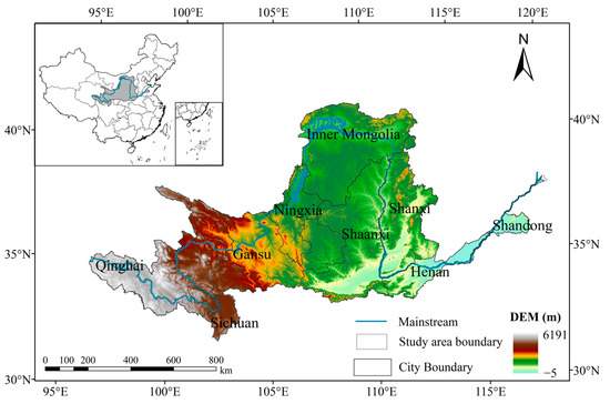
Figure 1.
The location and elevation of the Yellow River Basin, China.
2.2. Datasets
2.2.1. Land Use/Cover Data
This study utilized a multi-period land use remote sensing monitoring dataset [38] from the Resource and Environment Science Data Platform (https://www.resdc.cn/, accessed on 19 July 2024). This dataset used Landsat remote sensing images as the main source of information, and a multi-period land use/land cover database was constructed through visual interpretation [39]. The dataset has covered 12 periods from 1980 to 2023, and each period of data has been generated based on the data of the previous period, with a spatial resolution of 30 m and a raster data format. The level is divided into six categories based on land resources and their utilization attributes, which are mainly divided into farmland (FL), woodland (WL), grassland (GL), water area (WA), construction land (CL), and unused land (UN).
2.2.2. Climate Factor Datasets
This study utilized a national collection of surface meteorological observations provided by the China Meteorological Administration (http://data.cma.cn, accessed on 10 June 2023), which covers mainland China and surrounding areas and contains more than 2400 national-level surface meteorological stations [36,40]. This data information center provides meteorological information such as temperature (TEM), precipitation (PRE), evapotranspiration (ET), and wind speed. This study used the thin plate spline function interpolation to preprocess the climatic data. Solar radiation (SR) is obtained from the European Centre for Medium-Range Weather Forecasts’ (ECMWF) fifth-generation global atmospheric reanalysis dataset (ERA5, https://cds.climate.copernicus.eu/, accessed on 10 June 2023), which provides a variety of variables related to solar radiation and supports filtering of data by region, time, and variable [38]. The Quantile Mapping (QM) method was used to correct the bias of the ERA5 data, which significantly improved the accuracy of the data and the consistency with the observed data.
2.2.3. Socio-Economic Data
Gross Domestic Product (GDP) is a key socio-economic indicator (Add), which was obtained through the Spatiotemporal Tripolar Environmental Big Data platform (https://portal.casearth.cn/poles, accessed on 15 June 2024), with a spatial resolution of 1 km and a temporal range from 2000 years to the present. Population density (POP) data are Worldpop kilometer-scale raster data with a spatial resolution of 30 arcseconds (about 1 km) and a temporal resolution of years [24]. The population density raster dataset is available for free on the official Worldpop website (https://www.worldpop.org/, accessed on 19 July 2022).
2.2.4. Vegetation Remote Sensing Datasets
The GIMMS NDVI3g remote sensing data released by NASA’s Global Monitoring and Modeling Research Group (https://gml.noaa.gov/, accessed on 19 June 2024) were used in this study, with a temporal resolution of 15 days and a spatial resolution of 8 km. The NDVI data were preprocessed using the maximum value synthesis method for each pixel to synthesize the monthly data. And the Savitzky–Golay method was used to remove high-frequency noise from each image of remote sensing, and smoothing and denoising were realized at the same time. This dataset significantly improves the spatial and temporal consistency of vegetation monitoring through improved sensor calibration and atmospheric correction methods and is particularly suitable for analyzing long-term vegetation trends at global or regional scales [41]. The gross primary productivity (GPP) and leaf area index (LAI) datasets [42] were provided by GLASS (http://glass.umd.edu/, accessed on 19 June 2024), which was compared with the global 300+ flux tower (FLUXNET) data (Add), with an accuracy validation of R2 from 0.7 to 0.9. Nearest Neighbor Interpolation was used to maintain a uniform spatial resolution of the remote sensing images of NDVI, GPP, and LUCC.
2.2.5. Geographic Data
Digital Elevation Model (DEM) and Slope data are from NASA (https://search.earthdata.nasa.gov, accessed on 10 July 2022). DEM and Slope data are fundamental datasets for terrain analysis and earth science research and are widely used in geomorphological research, hydrological modeling, disaster assessment, and other fields [37,43]. NASA provides multi-resolution DEM products through multi-mission satellites and remote sensing technology and supports Slope calculation based on DEM.
2.3. Methods
The technical roadmap is divided into three components: land use changes and driving factors, the scenario simulation process of land use and habitat quality, and the analysis of their coupling relationship (Figure 2).
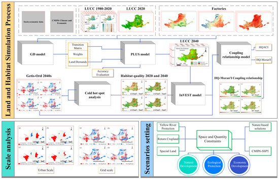
Figure 2.
The technical roadmap.
2.3.1. Land Use Transfer Matrix
Land use transfer matrices have been used to quantify the inter-class conversions across temporal periods, which visualize the direction and amount of change in land types [23,24]. Land use transfer matrices typically show the conversion between various land types between two points in time in the form of a matrix. The rows of the matrix represent the land types at the initial point in time, the columns represent the land types at the end point in time, and the value of each cell represents the area or proportion of land that has been converted from the row type to the column type. The mathematical formula is
Assuming that the land types in the study area are categorized into type y, the categorized data at different times are formed into a matrix of x × y. denotes the area converted from type x to type y.
Where is the degree of change in land use type m; denotes the absolute value of the change in land between type m and type n; represents the area of a; and t denotes the length of time.
2.3.2. GeoDetector
GeoDetector is a statistical method based on the principle of spatial dissimilarity for detecting the spatial distribution patterns of geographic phenomena and their driving factors [44]. In this study, we selected topography (DEM and Slope), climatic factors (TEM, PRE, and SR), ecological indicators (LAI, NDVI, GPP, and ET), and socio-economic indicators (POP and GDP) for a total of eleven drivers, by using GeoDetector to reveal nonlinear synergistic or antagonistic effects among the multiple factors and to assess the differences in the impacts on the LUCC. The model does not require linear assumptions and has the advantage of dealing directly with categorized data.
where r = 1, …, N; L is the stratification of variable Y or factor X; and r are the number of cells in layer h and the whole region, respectively; and and are the variances of the Y-values for layer r and the whole region, respectively. The q-value measures the explanatory power of factor X on the geographic phenomenon Y. It ranges between [0 and 1], with larger values indicating that X has a stronger influence on Y.
2.3.3. Markov Chain
Markov Chain is a probabilistic model that describes the state transfer of a stochastic process, and its central feature is that it satisfies no posteriority [45]. The method considered land types as discrete states and quantified the inter-transformation laws among different types by constructing a state transfer probability matrix, thereby predicting future land cover patterns [46].
where N is the total number of land use types, and j is the transfer probability of being in state i at moment t.
2.3.4. Patch-Generating Land Use Simulation (PLUS)
The PLUS model is a metacellular automata-based land use simulation tool that enables high-precision simulation of LUCC at the patch level by integrating the Random Forest algorithm and a multi-type random patch seeding mechanism [47]. The core steps include data preprocessing, land expansion strategy analysis, multi-scenario parameterization, and dynamic simulation, which supports the combination of Markov Chain to forecast land demand, output spatial pattern, and statistical indicators and is widely used in land use driving factors analysis and LUCC simulation [48]. The calculation formula is as follows:
where is the total number of type k targets predicted by the Markov Chain; is the difference between the current number of converted class k image elements and the target amount.
Based on the PLUS model, this study integrates a total of 11 categories of driving factors, including topography (DEM, Slope), climatic factors (TEM, PRE, SR), ecological indicators (LAI, NDVI, GPP, ET), and socio-economic factors (POP, GDP). The Land Extension Analysis Strategy (LEAS) was used to excavate the driving mechanisms of land type changes in the YRB from 1980 to 2020 and to quantify the contributions of the drivers. Validation results demonstrate that under these parameters, the model achieves a Kappa Coefficient of 0.92 and an Overall Accuracy of 95.8%.
Three land use change scenarios were simulated: (1) Natural development scenario, where land use evolution follows historical transition patterns under past socio-economic conditions. This research assumes the persistence of historical growth patterns over the coming decades, thus maintaining all transition probabilities without imposing restriction parameters in simulation experiments. (2) The ecological protection scenario emphasizes ecological conservation through strategic adjustments to land use transition probabilities in the YRB. Specifically, the transition probability from farmland to forest land is increased by 30% and to grassland by 60%, while it is reduced by 50% for conversion to construction land. For woodland, transition probabilities to farmland and grassland are decreased by 80%, with a 90% reduction in conversion probability to construction land. Grassland demonstrates a 20% increase in transition probability to farmland and an 80% decrease in conversion to construction land. Regarding unused land, transition probabilities to farmland and woodland are both elevated by 20%, with a 50% increase in conversion probability to grassland. All other inter-category transition probabilities remain unadjusted. The transition probability adjustments explicitly enhance carbon sink capacities through afforestation and grassland restoration, serving as nature-based solutions (NbSs) to achieve climate stabilization targets. Increased woodland conversion ratios are calibrated to offset projected temperature-induced carbon loss under RCP4.5 scenarios. (3) The economic development scenario, aligned with the economic growth objectives of the United Nations Sustainable Development Goals (SDGs), permits unrestricted urban expansion. Based on the land use transfer matrix, transition probabilities are configured as follows: conversion from farmland to construction land increases by 60%, grassland to construction land rises by 50%, and unused land to construction land grows by 30%. Transition probabilities between other land categories remain unaltered. This high-intensity development configuration corresponds to CMIP6-SSP5-driven climate pathways, where accelerated urbanization reflects carbon-intensive industrialization patterns. Unrestricted construction land expansion simulates warming-aggravated land demand under business-as-usual emission scenarios, while retained conversion parameters account for climate-adaptive land use trade-offs.
2.3.5. Habitat Quality Assessment (HQA) Based on InVEST Model
Habitat quality, defined as the capacity of an environment to provide suitable conditions for the survival and reproduction of individuals and populations, serves as a foundational indicator of biodiversity and a critical ecosystem service. Assessing regional habitat quality provides scientific insights for biodiversity conservation and ecological protection strategies, particularly in understanding the impacts of land use transformation on habitat dynamics. The Integrated Valuation of Ecosystem Services and Trade-Offs (InVEST) model was employed to quantify habitat quality by integrating the spatial distribution of habitat threats and the sensitivity of different land use types to these threats. This approach enables systematic evaluation of how land use changes influence habitat degradation or improvement.
The InVEST habitat quality module computes habitat quality scores based on the following core formula
where is habitat quality index for grid cell x in land use/land cover (LULC) type ; is habitat suitability score (0–1) for LULC type ; is total threat level to habitat in grid cell ; is half-saturation constant (set to 0.5 by default); and is scaling parameter (typically 2.5).
2.3.6. Anselin Local Moran’s I
To elucidate the spatial clustering patterns and temporal evolution of habitat quality under land use transitions, a Local Indicators of Spatial Association (LISA) analysis was performed using Anselin Local Moran’s I. This method identifies statistically significant spatial clusters and outliers in habitat quality distributions across both current and future simulated scenarios. The analysis quantifies local spatial autocorrelation, revealing regions where high or low habitat quality values exhibit significant spatial aggregation or divergence.
For each temporal phase (current year and future projection), habitat quality indices derived from the InVEST model were standardized to z-scores. A spatial weights matrix was constructed based on queen contiguity to define neighborhood relationships among grid cells. The Local Moran’s I statistic for grid cell is expressed as
where is habitat quality value at cell ; is mean habitat quality across all cells; is variance of habitat quality values; is spatial weight between cells and (1 for neighbors, 0 otherwise); and is total number of cells.
Significance testing (p < 0.05) was conducted using 999 permutations to classify spatial clusters into four categories:
High–High (H-H): High habitat quality cells surrounded by high-quality neighbors;
Low–Low (L-L): Low habitat quality cells surrounded by low-quality neighbors;
High–Low (H-L): High habitat quality cells adjacent to low-quality areas;
Low–High (L-H): Low habitat quality cells adjacent to high-quality areas.
Spatiotemporal changes in clustering patterns were analyzed by comparing LISA maps between current and future scenarios. This approach delineates regions where habitat quality degradation or improvement exhibits spatial dependency, offering insights into the localized impacts of land use transitions. The results were visualized using GIS tools to highlight critical areas requiring prioritized conservation interventions.
2.3.7. Habitat Quality–Autocorrelated Coupling Index (HQACI)
To assess the synergistic relationship between habitat quality differentiation and agglomeration patterns, a Habitat Quality–Autocorrelated Coupling Index (HQACI) was proposed and calculated as follows:
where and represent the spatial extents of statistically significant (p < 0.05) H-H and L-L clusters derived from the Local Moran’s I analysis. denotes the total area of the study region.
The H-H and L-L clusters were extracted using GIS spatial query tools based on significance levels (p-value) and cluster-type attributes. Area calculations were performed using the zonal statistics module to ensure alignment with the habitat quality raster resolution.
The HQACI quantifies the proportion of the study area where spatial differentiation (habitat quality gradients) coincides with significant agglomeration effects. A higher CI value (range: 0−100%) indicates stronger synergy between habitat quality heterogeneity and spatial autocorrelation, suggesting that high- or low-value regions tend to cluster cohesively. This metric helps identify zones where conservation policies or restoration efforts could maximize ecological benefits.
3. Results
3.1. Characteristics of the Spatial and Temporal Evolution of LUCC in the YRB
3.1.1. Temporal Characteristics of LUCC
This study employed multi-temporal LUCC remote sensing monitoring datasets to conduct a raster-based analysis and calculated area variations in principal land use types in the YRB from 1980 to 2020 for each raster (Figure 3). The temporal dynamics of different LUCCs were statistically analyzed across distinct observation periods, with quantitative results systematically presented in Figure 3 and Table 1. From 1982 to 2020, the water area, farmland, and unused land decreased, and woodland, grassland, and construction land showed an increasing trend, in which the area of farmland was transferred out of 86,442.19 km2, and forest land and grassland increased by 3737.68 km2 and 1824.47 km2, respectively; and the construction land increased by 12,941.77 km2. From 1980 to 2000, the areas of farmland, woodland, and construction land increased, while the areas of the grassland, water area, and unused land all decreased by 2697.13 km2, 1678.92 km2, and 488.36 km2, respectively. The comparison of 2000–2020 and 1980–2000 found that the areas of the woodland, grassland, water area, and construction land increased, of which the forest land, grassland, and construction land showed an upward trend from 2000 to 2020, increasing by 3474.67 km2, 4521.61 km2, and 11166.15 km2, respectively. The area of farmland and unused land decreased, and the decrease in unused land (7772.85 km2) was significantly lower than the decrease in farmland (12,570.87 km2).
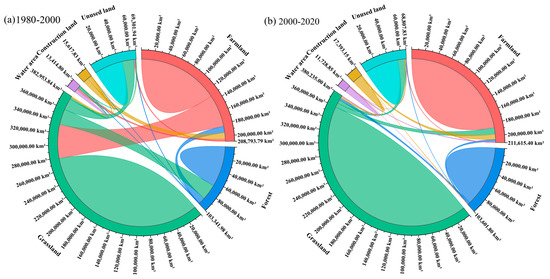
Figure 3.
Temporal characteristics of LUCC in the YRB. (a) 1980–2000 and (b) 2000–2020.

Table 1.
The transfer matrix of land use changes in the YRB from 1980 to 2020.
3.1.2. Spatial Characteristics of Land Use Transfer
The LUCC transfer matrix was used to analyze the LUCC of each raster at different time periods. According to the spatial variation characteristics of the LUCC transfer in different time periods in Figure 4, it is found that LUCC shows significant regional heterogeneity in the YRB. From 1980 to 2020, the farmland and unused land decreased by 9747.98 km2 and 8261.20 km2, respectively, and the main conversion types included the conversion of farmland to woodland (11,762.12 km2), unused land to woodland (1283.78 km2), unused land to grassland (24,008.14 km2), and other types of changes. LUCCs are more pronounced in Gansu, southern Shaanxi, southwestern Shanxi, and Inner Mongolia. A large amount of grassland, woodland, and unused land was reclaimed as farmland during the period of 1982–2000, and the water area and unused land decreased by 1678.92 km2 and 488.36 km2, respectively, which were mainly located in the Loess Plateau area in the central part of the study area.
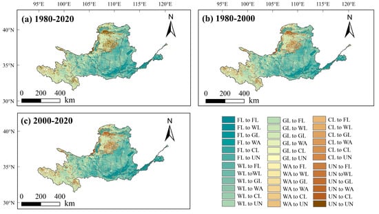
Figure 4.
Characteristics of the spatial change in the LUCC in the Yellow River Basin. (a) 1980–2020; (b) 1980–2000; and (c) 2000–2020.
The statistical results of the LUCC transfer matrix (Figure 5) show that after 2000–2020, along with the implementation of the policy of returning the farmland to forests and grasslands, a large area of farmland in the Yellow River Basin was converted from farmland to woodland (3234.01 km2) and grassland (10,820.45 km2), and the areas of woodland and grassland increased by 3474.67 km2 and 4521.61 km2, respectively, from 2000 to 2020, and 4521.61 km2 was mainly distributed in the Loess Plateau area in the central part of the YRB. The conversion of unused land to cropland, woodland, grassland, and construction land exists in the Inner Mongolia region in the northern part of the Yellow River Basin. Construction land is continuously expanding, mainly in the Henan and Shandong regions.
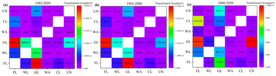
Figure 5.
Characteristics of the LUCC in the YRB in different periods. (a) 1980–2020; (b) 1980–2000; and (c) 2000–2020.
3.2. Analysis of Driving Factors for LUCC
3.2.1. The Analysis of the Influence Factor Detector Results
Quantifying the driving factors of land use change based on the PLUS model (Figure 6), the results indicated that the changes in the farmland area were mainly driven by the POP (0.148) and GDP (0.129). There is a significant correlation between the PRE (0.098) and DEM (0.087), which indicates that the evolution of farmland is a consequence of the combination of socio-economic demands and natural environmental conditions. The expansion of construction land is most strongly influenced by the socio-economic dimension, with the POP coefficient reaching 0.282 and the GDP coefficient reaching 0.153. The woodland changes were strongly influenced by multiple factors, with the ET (0.122), POP (0.133), and GDP (0.116) as major driving factors, and the natural restoration effect of the NDVI (0.095) as a secondary driving factor, which indicates that the forestry development was simultaneously influenced by both the ecological project implementation and regional economic restructuring.
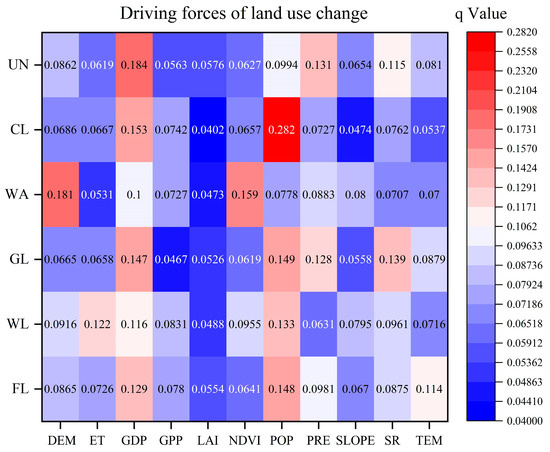
Figure 6.
Driving forces of land use change from 2000 to 2020.
The driving mechanisms of the grassland ecosystem are more complex, and in addition to the socio-economic pressures of the POP and GDP, climatic factors such as SR (0.139) and PRE (0.128) show a strong explanatory power, suggesting that grassland changes in high-altitude regions are more sensitive to the climate. The water area changes showed significant topographic dependence, with a DEM driving coefficient of 0.181, which, combined with the influence of the NDVI (0.159), suggests that the geomorphic characteristics of the riparian zone and the vegetation cover status are important constraints on the spatial differentiation of the watershed. The expansion of construction land shows significant socio-economic driving characteristics, with a POP coefficient of 0.282, which is significantly higher than that of other land categories, reflecting the main driving force of the population agglomeration effect on land development in the process of urbanization. The contribution rate of the GDP factor is 0.153, which forms a gradient difference with the farmland (0.129) and the woodland (0.116), demonstrating that there is a strong spatial matching characteristic between the growth of the construction land and regional economic activities. The evolution of unused land exhibits a driving pattern dominated by the GDP (0.184) and is superimposed on the natural condition constraints of PRE (0.131) and SR (0.115), which shows that there is a penetration of economic factors into the unused land in the process of regional development.
3.2.2. Analysis of Interaction Detector Results
From the interaction level of the main influencing factors, there are six types of factors, the ET, NDVI, PRE, LAI, GPP, and GDP (Figure 7), which constitute the main driving group, and their average interaction explanatory power is more than 0.08, which has the main influence on the macro-patterns of the land use in the YRB. Among them, the coupling of climatic and topographic elements showed significant spatial differentiation. The interaction effect between PRE and ET (0.138) indicates that precipitation drives the gradient differentiation pattern of land cover types by changing the intensity of the regional moisture cycle. The interaction explanatory power of SLOPE and the DEM reaches 0.1155, suggesting that topographic relief and elevation jointly suppress the intensity of human activities in high-elevation areas. The interaction between the GDP and GPP (0.1045) demonstrates that construction land expands outward along high-productivity vegetation areas under their synergistic effects. The strong interaction between the LAI and GPP (0.102) demonstrates that their synergistic effects promote agricultural land intensification.
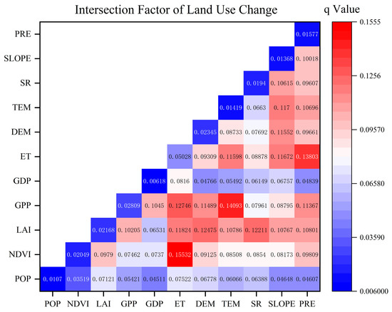
Figure 7.
Interaction factors of land use change from 2000 to 2020.
From the perspective of secondary driver interactions, the DEM, SLOPE, and TEM as a secondary driver group exhibit an interaction explanatory power of 0.07–0.09 through topographic barrier effects and thermal condition regulation, indicating their interactions exert a limited influence on land use changes. While the independent effects of SR and the POP remain weak, their synergistic effects with climatic factors (0.088) suggest that light–thermal resource combinations may shape the spatial allocation of farmland.
3.3. The Scenario Simulation of the LUCC in the Yellow River Basin
3.3.1. Scenario Simulation of LUCC in 2040
In order to examine the future land use demand under different scenarios and the impact of policy control on LUCC, this study sets up three scenarios of natural development, ecological protection, and economic development to simulate the LUCC in the YRB (Figure 8 and Figure 9). The spatial distribution and statistical results of land use changes under the simulation of natural development scenarios in 2040 (Figure 8 and Table 2) reveal that there are differences in the spatial heterogeneity of different vegetation types. Farmland, woodland, and grassland areas are significantly higher than other types, with grassland accounting for the highest proportion of the total study area (49.01%), followed by farmland (23.77%) and woodland (13.77%). Grassland and woodland are mainly distributed in the regions of Qinghai, Shanxi, and Inner Mongolia, while the unused land (55,993.19 km2, 7.01%) is mainly distributed in the regions of Qinghai, Inner Mongolia, and northern Shaanxi. The construction land (37,769.38 km2, 4.73%) is mainly distributed in southern Shaanxi, Shanxi, Henan, and Shandong.

Figure 8.
The simulation of the land use change under the natural development scenario for the Yellow River Basin in 2040.
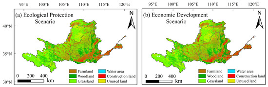
Figure 9.
The simulation of land use changes under the ecological protection scenario (a) and the economic development scenario (b) of the Yellow River Basin in 2040.
Table 2.
Statistics of changes under different simulation scenarios for different land use types in 2040.
The spatial distribution characteristics of LUCC under the ecological protection scenario and the economic development scenario are similar (Figure 9), with grasslands and woodlands mainly concentrated in Qinghai, Sichuan, and Gansu in the upstream of the YRB, as well as in Ningxia, Shanxi, and Inner Mongolia in the middle of the YRB. The order of different vegetation types in the total study area under the different scenarios, from highest to lowest, was grassland > farmland > woodland > unused land > constructed land > water area. However, woodland (13.88%) and grassland (50.35) areas under the ecological protection scenario were higher than woodland (12.50%) and grassland (49.62%) areas under the economic development scenario. The area of construction land under the economic development scenario (5.10%) is higher than that of the ecological protection scenario (3.85%) and natural development scenario (4.73%). The spatial distribution of the construction land is more obvious, mainly concentrated in Shaanxi, Shanxi, Henan, and Shandong.
3.3.2. The Analysis of the Results of the LUCC from 2020 to 2040
The results of the LUCC transfer matrix from 2020 to 2040 found (Figure 10) that the area of the farmland and unused land under the natural development scenario decreased by 17,867.39 km2 and 11,015.90 km2, respectively. And the decrease in unused land was significantly lower than that of farmland, with farmland decreasing by the highest amount. At the same time, the areas of woodland, grassland, water bodies, and construction land show an increasing trend. The farmland and unused land under the ecological protection scenario and the economic development scenario also show a decreasing trend, while the areas of the woodland, grassland, water area, and construction land show an increasing trend, which is similar to that under the natural development scenario. However, the area of woodland increased by 7229.66 km2 under the ecological conservation scenario, which was higher than that of the economic development scenario (2984.41 km2). The proportions of farmland, woodland, and grassland in the total study area under the ecological conservation scenario model were 19.04%, 11.94%, and 48.01%, respectively. The proportions of farmland, woodland, grassland, and construction land in the total study area under the economic development scenario were 18.59%, 11.16%, 35.07%, and 21.57%, respectively. The area of the increased grassland is higher in the ecological conservation scenario (48.01%) than in the economic development scenario (35.07%), with a relative increase of 12.94%. The construction land is significantly higher in the economic development scenario (21.57%) than in the ecological protection scenario (7.73%), with a relative increase of 13.84%.

Figure 10.
Land use change transfer matrix for three different scenarios from 2020 to 2040. (a) Natural development scenario; (b) ecological protection scenario; and (c) economic development scenario.
3.3.3. The LUCC of Nine Provinces in the YRB Under the Scenario Simulation
The LUCCs under the natural development scenario of nine different provinces in the Yellow River Basin are shown in Figure 11, and the land use types with a higher percentage of area are farmland, woodland, and grassland. Farmland areas are mainly distributed in the Shanxi, Henan, and Shandong provinces, amounting to 35,051.06 km2, 18,282.44 km2, and 7182.83 km2, respectively. Grassland areas are mainly distributed in Inner Mongolia and Qinghai regions, accounting for 80,459.30 km2 (10.08%) and 117,914.87 km2 (14.77%) of the YRB, respectively. The proportion of construction land is higher than other land use types in Shanxi, Henan, and Shandong, accounting for 7.69%, 13.68%, and 21.90%, respectively. Grassland occupies a higher proportion in Qinghai Province (74.53%) and Inner Mongolia (53.54%), accounting for 14.77% and 10.08% of the total study area, respectively. Some unused land existed in Sichuan, Inner Mongolia, Ningxia, and Qinghai, and the unused land in the Inner Mongolia region (29,406.53 km2, 3.68%) was higher than in the other eight provinces.
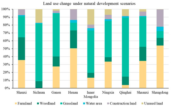
Figure 11.
Land use changes in different provinces under the natural development scenario in the Yellow River Basin in 2040.
Comparing the land use changes in the nine provinces under the ecological protection scenario and the economic development scenario (Figure 12), it is known that there are differences in the changes in land use types under different land use change scenarios. The main land use type in Sichuan, Gansu, Qinghai, and Inner Mongolia is grassland, and the main land use type in Henan and Shandong is cropland. Under the ecological protection scenario, grasslands in Sichuan, Gansu, Qinghai, and Inner Mongolia accounted for 73.93%, 56.30%, 75.63%, and 54.55% of their respective regions, respectively; farmland in Henan and Shandong accounted for 52.60% and 57.17% of the distribution in their respective regions; the regions with a higher proportion of woodland are Shanxi (29.32%) and Henan (22.80%); and construction land is widely distributed in Henan and Shandong, with the construction land in Shandong accounting for 17.34% of its total land category.
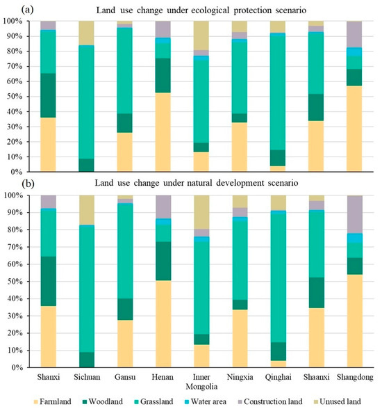
Figure 12.
Land use changes in different provinces under the ecological protection scenario (a) and the economic development scenario (b) in the Yellow River Basin in 2040.
Under the economic development scenario, the grassland in Sichuan, Gansu, Qinghai, and Inner Mongolia accounted for 72.55%, 54.25%, 74.46%, and 53.50% of their respective regions, which is slightly lower than the area of grassland under the nature conservation scenario; and the main land use type in Henan and Shandong was farmland, which accounted for 49.56% and 52.83% of their provinces, respectively. The regions with a higher proportion of construction land are Shandong (23.54%) and Henan (14.69%); the area of constructed land under the economic development scenario is relatively higher than that under the nature conservation scenario, which is 6.2% higher in Shandong Province and 3.45% higher in Henan Province. The proportion of unused land under the ecological protection scenario and the economic development scenario is the highest in the Inner Mongolia region, significantly higher than in other provinces, accounting for 19.58% and 19.16% of the Inner Mongolia region, respectively.
3.4. Habitat Quality: Spatial Heterogeneity and Local Autocorrelation Analysis
3.4.1. Spatial Distribution Patterns and Classification of Habitat Quality
Under current conditions (2020, Figure 13a), the habitat quality exhibits a heterogeneous spatial distribution, with high-value clusters (intense green, values ≈ 1) concentrated in the southwestern and southeastern basin, particularly along riparian corridors and mid-elevation plateaus. These zones likely correspond to intact forest ecosystems and regulated floodplains, where minimal anthropogenic disturbance preserves ecological functionality. Low-quality areas (values < 0.3) dominate the central basin, aligning with intensive cropland irrigation.
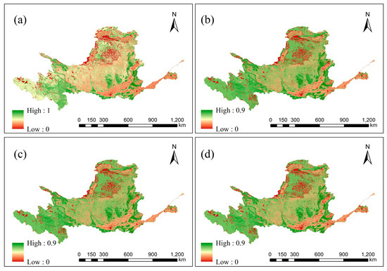
Figure 13.
An evaluation of the habitat quality in the Yellow River Basin: (a) The situation in 2020; (b) natural development simulation scenario in 2040; (c) the ecological protection scenario in 2040; and (d) the economic development simulation scenario in 2040.
Projections to 2040 under the natural development scenario (Figure 13b) demonstrate a discernible yet gradual quality decline, manifested through the expansion of orange–yellow transitional zones along the southern basin periphery. This suggests the encroachment of moderate-intensity land uses into formerly stable habitats. The retention of core high-quality clusters in the central–western highlands implies that topographic constraints buffer these areas from near-term development pressures.
The ecological protection scenario (Figure 13c) achieves spatial conservation efficacy, maintaining baseline high-quality areas relative to 2020. The enhanced green continuity along major tributaries indicates the successful implementation of riparian buffer policies, though persistent red patches in the Ordos Plateau highlight challenges in rehabilitating aridland ecosystems.
The economic development scenario (Figure 13d) generates a polarized landscape: sprawling low-quality zones engulf the northeastern basin, a probable consequence of prioritized industrial expansion, while isolated high-quality refugia persist in high-altitude reserves, reflecting geographically constrained conservation trade-offs.
3.4.2. Local Spatial Autocorrelation Characteristics of Habitat Quality
At the grid-scale 2020 baseline (Figure 14a), statistically significant H-H clusters dominate the central basin, particularly within riparian corridors and mid-elevation plateaus, suggesting the strong spatial aggregation of high-quality habitats in regions with balanced ecological and anthropogenic influences. These H-H clusters are interspersed with non-significant zones in transitional areas, reflecting a fragmented habitat connectivity. L-L clusters concentrate in the northeastern plains and southeastern margins, aligning with intensive agricultural activity.
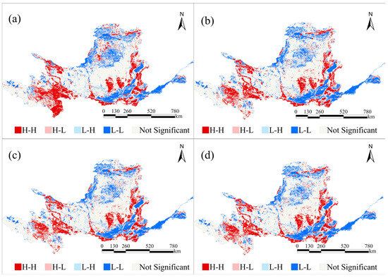
Figure 14.
Anselin Local Moran’s I results of the habitat quality assessment in the Yellow River Basin at the grid scale: (a) the current situation in 2020; (b) the natural development simulation scenario in 2040; (c) the ecological protection scenario in 2040; and (d) the economic development simulation scenario in 2040.
Under the 2040 natural development scenario (Figure 14b), the spatial coherence of H-H clusters diminishes, evidenced by the reduced red continuity and increased white interstitial areas. This fragmentation corresponds to the simulated unregulated land use expansion, particularly at urban–rural interfaces, where medium-intensity development disrupts habitat adjacency. Conversely, L-L clusters expand in the northeastern basin, likely driven by agricultural intensification and groundwater over-extraction. The spatial polarization between H-H and L-L zones intensifies, with a reduction in transitional (H-L/L-H) clusters, indicating homogenization pressures.
The ecological protection scenario (Figure 14c) demonstrates conservation efficacy, retaining a baseline H-H cluster area while reducing the L-L coverage. The enhanced red continuity along the Weihe and Fenhe river valleys reflects a successful riparian buffer implementation, though persistent L-L zones in the Ordos Plateau highlight enduring challenges in aridland restoration. Non-significant areas decrease, suggesting an improved habitat connectivity through policy-driven corridor establishment.
In contrast, the economic development scenario (Figure 14d) generates a bifurcated landscape: H-H clusters retreat to high-altitude refugia, while L-L zones proliferate across the northeastern basin, a consequence of prioritized industrial zoning and mineral extraction. H-L outliers emerge near provincial capitals, marking abrupt habitat quality transitions at urban peripheries.
The analysis results show two key trends. (1) Anthropogenic pressures drive asymmetric decoupling: economic prioritization disrupts upstream–downstream habitat linkages, disproportionately affecting lowland ecosystems; (2) conservation efficacy is spatially bounded: ecological policies stabilize core H-H clusters but show a limited penetration into arid and peri-urban zones.
At the urban scale 2020 baseline (Figure 15a), H-H clusters predominantly aggregate in the central and southwestern regions, likely corresponding to protected forest reserves and riparian ecosystems with minimal anthropogenic disturbance. These clusters are spatially juxtaposed with L-L clusters concentrated in the northeastern plains and peri-urban zones, reflecting intensive agricultural and industrial land uses. The presence of H-L outliers along transitional ecotones suggests localized habitat degradation encroaching on high-quality cores, while L-H outliers mark marginal areas with incipient ecological recovery potential.
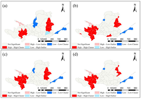
Figure 15.
Anselin Local Moran’s I results of the habitat quality assessment in the Yellow River Basin at the urban scale: (a) The current situation in 2020; (b) the natural development simulation scenario in 2040; (c) the ecological protection scenario in 2040; and (d) the economic development simulation scenario in 2040.
Projections to 2040 under the natural development scenario (Figure 15b) illustrate a spatial decoupling of habitat quality, characterized by the reduction in the H-H cluster continuity and the expansion of L-L clusters in the northeastern basin. This fragmentation aligns with the simulated urban sprawl and agricultural intensification, where non-significant zones have a few increases, indicating a disrupted spatial autocorrelation. The emergence of new H-L outliers underscores edge effects from unregulated land use transitions.
In contrast, the ecological protection scenario (Figure 15c) demonstrates the stabilization of H-H clusters, retaining their 2020 spatial extent, particularly along the Weihe and Fenhe river corridors. L-L clusters contract with significant reductions in the Ordos Plateau and northern agricultural plains, suggesting the effective mitigation of degradation through policy-driven habitat restoration. The near elimination of H-L outliers in ecotonal zones highlights an improved spatial coherence, though persistent L-H outliers in arid margins indicate lingering recovery challenges.
In the economic development scenario (Figure 15d) H-H clusters fragment, particularly in the northeast, as economic activities disrupt high-quality habitat agglomeration. L-L clusters show a potential contraction, suggesting that the reduction in low-quality habitat clusters may be due to the land use change prioritizing economic development over ecology. H-L outliers persist, with no reduction in spatial discontinuities, reflecting persistent trade-offs between economic growth and ecological integrity. The results reveal the macroscale homogenization of L-L zones in the northeastern basin versus microscale fragmentation in southwestern mountainous regions.
3.4.3. Interplay Between Spatial Heterogeneity and Autocorrelation Patterns
The spatial autocorrelation analysis of the habitat quality across development scenarios reveals distinct spatial heterogeneity characteristics in the Yellow River Basin (Figure 16 and Table 3). Under the current scenario, medium-quality habitats dominate (34.71%), followed by low-quality (19.59%) and high-quality (8.24%) areas, forming a hierarchical quality structure. Scenario simulations demonstrate significant spatial reorganization, with the ecological protection scenario achieving optimal conservation outcomes through a 39.78 percentage point expansion of high-quality non-significant areas (48.02%) and a concurrent reduction in low-quality zones to 3.10%. This contrasts sharply with the economic development scenario, which manifests increased L-L clustering in medium-quality habitats (8.86% vs. 1.57% baseline) and elevated H-L outliers in high-quality areas (0.17% vs. 0.03% baseline), which is indicative of localized habitat degradation near economic hubs.

Figure 16.
The analysis of the correlation between the habitat quality and local spatial autocorrelation: (a) the current situation in 2020; (b) the natural development simulation scenario in 2040; (c) the ecological protection scenario in 2040; and (d) the economic development simulation scenario in 2040.
Table 3.
Habitat quality–local spatial autocorrelation combination and area proportion.
Spatial autocorrelation patterns exhibit quality-dependent clustering behaviors. High-quality habitats maintain stable H-H cluster proportions (16.15–16.18% across scenarios), confirming the spatial resilience of core ecological zones. Conversely, low-quality areas show scenario-sensitive L-L cluster dynamics, decreasing from 8.66% under current conditions to 0.78% in ecological protection scenarios, illustrating the effective mitigation of low-value aggregation through conservation measures. Spatial outliers remain marginal (<0.3% overall), though their distribution shifts reveal scenario-specific pressures: economic development induces 0.17% H-L anomalies in high-quality regions, while natural progression scenarios generate intermediate outlier distributions.
The ecological protection scenario demonstrates a superior performance in both quality enhancement and spatial pattern optimization, reducing low-quality L-L clusters by 7.89 percentage points and expanding high-quality non-significant areas to 48.02%. This contrasts with the economic development scenario’s paradoxical effects: while marginally improving some medium-quality indicators, it increases H-L outliers in high-quality zones, suggesting intensified edge effects near development corridors. Natural development scenarios present transitional characteristics, maintaining the baseline H-H cluster stability (16.15%) but showing a limited capacity for quality hierarchy improvement.
Strategic recommendations emphasize three spatial interventions: establishing ecological corridors between stable H-H clusters (16.58% coverage) to enhance connectivity; implementing targeted restoration in persistent L-L clusters (8.66% in low-quality areas), particularly in agricultural–urban transition zones; and instituting development intensity thresholds in H-L anomaly concentrations (0.17% in economic scenarios) to prevent habitat fragmentation. These findings quantitatively validate the spatial efficacy of ecological conservation strategies while highlighting the need for differentiated zoning controls to balance development pressures in this ecologically sensitive watershed.
The HQACI quantifies the spatial synergy between the habitat quality differentiation and clustering patterns (Table 4), with values ranging from zero (no synergy) to one (complete synergy). In the Yellow River Basin, the baseline HQACI in 2020 is 0.373, indicating moderate spatial coupling, where high-quality habitats and low-quality habitats exhibit localized clustering but lack a basin-wide coherence. By 2040, projected scenarios reveal a consistent decline in the HQACI across all developmental pathways, signaling a weakening synergy between habitat heterogeneity and agglomeration effects.
Table 4.
Habitat Quality–Autocorrelated Coupling Index of YRB.
Under the current conditions (2020 HQACI = 0.3728), the baseline HQACI reflects a landscape where habitat quality clusters are partially influenced by natural gradients and anthropogenic activities. High-quality clusters (H-H) likely coincide with protected zones or less disturbed ecosystems, while low-quality clusters (L-L) align with urban expansion and agricultural intensification. However, the moderate coupling value suggests a significant intermixing of habitat types, limiting the dominance of cohesive ecological cores.
Under the natural development scenario (HQACI = 0.3489, −6.2% from 2020), the marginal decline under this scenario implies that continued land use trends further fragment habitats, dispersing H-H clusters and expanding L-L zones. The spatial decoupling may arise from unregulated encroachment into ecologically sensitive areas, such as riparian buffers or grassland peripheries.
Under the ecological protection scenario (HQACI = 0.3450, −7.4% from 2020), despite conservation efforts, the lowest HQACI highlights limitations in isolated protection strategies. Protected areas may fail to mitigate edge effects from adjacent developed regions, leading to habitat degradation in transitional zones. This underscores the need for landscape-scale connectivity rather than fragmented reserves.
Under the economic development scenario (HQACI = 0.3488, −6.3% from 2020), the similarity to the natural development scenario suggests that economic priorities offset potential ecological gains. Intensive resource extraction in regions like the Loess Plateau could degrade the soil and vegetation, dispersing L-L clusters and eroding high-quality habitat nuclei.
The minimal variation among scenarios (ΔHQACI < 0.004) reveals systemic challenges in balancing conservation and development. The persistent decline across all pathways points to ecological homogenization, a trend where the habitat quality becomes more uniformly distributed but at lower overall levels, reducing the resilience to environmental stressors. This homogenization may stem from overlapping pressures: climate-driven aridification in upstream regions, groundwater depletion in mid-basin agricultural hubs, and downstream coastal urbanization.
4. Discussion
4.1. Characteristics of the Land Use Change in the Yellow River Basin
Changes in spatial and temporal patterns of land use in the Yellow River Basin indicated that farmland decreased after 2000, and the reduced area of farmland was mainly transformed into woodland and grassland (accounting for 58% and 37%, respectively). The reduction in the farmland area is to a large extent closely related to the implementation of the policy of returning farmland to woodland and grassland [8,27,49]. Compared with the Yangtze River Basin, the rate of farmland loss in the YRB is more rapid, mainly due to the double squeezing effect of ecological restoration and accelerated urbanization [22,50]. The area of woodland and grassland increased by 3474.67 km2 and 4521.61 km2, respectively, and the effect of ecological restoration was particularly significant in the Loess Plateau region. Woodlands are mainly distributed in the mountainous and hilly areas of the western part of Henan Province, the Taihang Mountains of the northwestern part of Henan Province, and the Dabie Mountains and Tongbai Mountains of the southern part of Henan Province, indicating that the ecosystems of woodlands and grasslands have been significantly improved under the implementation of ecological restoration projects and the implementation of the policy of returning farmland to forests and grasslands [5,15,49]. Many scholars have focused on policy-driven regional characteristics [2,43,51,52]. Liu et al. [3] found that China’s farmland showed a trend of a “decrease in the south and increase in the north” from 1990 to 2010, with the center of gravity of new farmland shifting from the northeast to the northwest and construction land in urban and rural areas accelerating on the east coast, which has been attributed to the pressures of urbanization and agricultural modernization. The proportion of farmland converted to woodland and grassland is higher in the Shaanxi, Shanxi, and Inner Mongolia regions in the middle part of the YRB, which reflects the remarkable spatial effectiveness under the implementation of the project of returning farmland to forest and grassland [8,15]. There are large areas that are converted from unused land to grassland (24,008.14 km2) in Qinghai and Gansu in the upstream region of the YRB, with vegetation restoration dominated by natural climate warming and wetting and policy-driven ecological engineering. The construction land expanded obviously in the downstream area of the YRB, and the contradiction between the expansion of urban agglomerations and food production became prominent [22,52,53], and the relationship between people and land became more strained.
Compared with the Yangtze River Basin (YtRB), land use changes in the YRB exhibited stronger policy-oriented characteristics. The rate of the farmland reduction from 2000 to 2020 in the YtRB (0.12%/a) is significantly lower than that in the YRB (0.35%/a) [54], and this difference results from the different development orientations of the two basins. The Yangtze River Economic Belt, as the main grain-producing area of the country, has maintained the dynamic stability of the total amount of farmland through the policy of the farmland compensation balance, while the ecological priority strategy of the YRB has prompted the conversion of larger-scale farmland into ecological land. The ecological restoration effectiveness of the YRB has remarkable particularities in comparison with semi-arid regions around the globe [2]. The rate of farmland loss in the Mediterranean climate zone from 2000 to 2020 (0.28%/a) was similar to that of the YRB, but its main driving factor was land desertification caused by climate change [55], whereas the vegetation cover in the YRB increased by 12.7% during the same period, which was attributed to the implementation of the largest systematic ecological project in the world [36,37]. Although the semi-arid region of the Midwest of the United States has maintained the stability of farmland through conservation tillage, its grassland area was still decreasing at a rate of 0.15%/a, which contrasts with the increase in grassland in the YRB, highlighting the unique effectiveness of China’s ecological restoration policy.
The simulation of future scenarios of land use in the YRB has revealed the divergent responses of the land system under different policy orientations [51,56,57]. In the ecological protection scenario, the significant increase in the woodland and grassland area indicates that the policy of returning farmland to forest and grassland can effectively promote ecological restoration, especially in the Loess Plateau and the upstream high-altitude area, and the continuous improvement of the vegetation cover will enhance the function of soil and water conservation [58,59,60]. However, the unused land has a potential risk of desertification and needs to be strengthened with ecological engineering. Under the economic development scenario, the rapid expansion of land for construction and the simultaneous increase in the loss of farmland have highlighted the contradiction between urbanization and agricultural production [61,62]. The proportion of construction land in the downstream plains (e.g., Henan and Shandong) exceeds 20%, reflecting the strengthening of the economic agglomeration effect on the centralized development of land resources. Overall, the complexity of the multi-scale driving mechanism requires that policy design needs to take into account the integration of natural constraints, economic aspirations, and engineering technologies in order to realize the sustainable transformation of the land system.
4.2. The Analysis of the Influencing Factors of the Land Use Change in the Yellow River Basin
This study systematically reveals the compound driving mechanisms and spatial operational patterns of land use changes in the YRB through the integration of the PLUS model and the GeoDetector methodology. The expansion of construction land was primarily driven by population agglomeration (q = 0.282) and economic development (q = 0.153), which is strongly associated with the rapid urbanization processes in core urban agglomerations across the basin [24,31,43]. This spatial pattern aligns with the fundamental characteristics of the YRB, where approximately 89.6% of the population concentrates in downstream and tributary valley areas (occupying 42.3% of the basin’s total area), leading to spatial mismatches between land development demands and the ecological carrying capacity, intensifying human–land system tensions. Farmland changes demonstrate compound driving mechanisms involving socio-economic factors (POP = 0.148, GDP = 0.129) and natural elements (PRE = 0.098, DEM = 0.087), reflecting the fundamental principle that agricultural production activities are subject to dual constraints of resource availability and environmental conditions [63,64]. The evolution of unused land exhibits a distinct economy-dominated pattern (GDP = 0.184), which may correlate with resource exploitation activities in ecologically fragile zones within the basin [24,44,60].
The multi-factor interaction analysis revealed the intrinsic complexity of the land system evolution. The ecological factor combination (ET∩NDVI = 0.155) exhibited the highest explanatory power, demonstrating that the synergistic effects of vegetation restoration and hydrological processes play a decisive role in land cover changes [3,65,66]. The climate–topography interactions (PRE∩ET = 0.138, SLOPE∩DEM = 0.1155) create natural barrier effects that effectively suppress the human activity intensity in high-elevation steep-slope areas. Conversely, the economy–ecology interactions (GDP∩GPP = 0.1045) reveal a potential risk of cropland resource loss exacerbated by the construction land expansion along high-productivity vegetation zones [28,67]. These findings align with the implementation efficacy of ecological conservation projects in the YRB [19,52,56,63,68]. Particularly in the Grain for Green Program (GFGP) implementation zones, the strong interaction between the NDVI and ET (0.155) substantiates vegetation restoration’s constraining effect on the land development intensity. It is recommended that the uncontrolled expansion of construction land be mitigated through the optimization of spatial arrangements. High-standard farmland construction should be strengthened to enhance the resilience of farmland resources, taking into account changes in precipitation patterns and topographical constraints in agricultural production areas. The management of ecologically fragile areas should focus on the synergistic improvement of the vegetation cover and hydrological conditions.
4.3. Spatiotemporal Patterns and Adaptive Management of Habitat Quality Clustering
The persistence of H-H clusters in the central and southwestern regions under all scenarios underscores the resilience of ecosystems in topographically complex zones, likely buffered by natural barriers against encroachment [69,70]. Conversely, the pervasive expansion of L-L clusters in the northeastern plains aligns with intensified agricultural and industrial activities, reflecting a systemic vulnerability of lowland habitats to development pressures. The ecological protection scenario mitigates the L-L cluster proliferation by 27%, demonstrating the potential of targeted conservation to counteract degradation trends, though its limited efficacy in arid margins highlights persistent challenges in balancing ecological restoration with climatic constraints [71].
The emergence of H-L outliers near urban peripheries across scenarios, particularly under economic prioritization, signals abrupt habitat quality transitions at development frontiers. These outliers, often marking interface zones between conserved and converted lands, emphasize the need for buffer strategies to dampen edge effects [72]. The stability of H-H clusters along riparian corridors, even amidst economic expansion, reinforces the dual role of river networks as both ecological lifelines and vectors of human influence [73], necessitating integrated watershed management to sustain connectivity.
The spatiotemporal analysis further identifies a threshold as a critical juncture where the L-L dominance transitions to mixed clustering patterns. This threshold corresponds to gradients in accessibility and resource exploitation intensity, suggesting that habitat quality responses are nonlinearly tied to proximity drivers [74]. The observed macroscale homogenization of L-L zones versus the microscale fragmentation in mountainous regions underscores the scale-dependent nature of conservation planning [75], advocating for multi-tiered governance frameworks.
These findings advocate for spatially adaptive interventions: fortifying H-H corridors in the central basin to maintain ecological coherence [76], implementing gradient restoration in transitional ecotones [77], and enforcing strict zoning within 50 km of urban H-L frontiers [78]. Future efforts must reconcile the basin’s role as an ecological refuge and economic engine, prioritizing policies that harmonize hydrological connectivity with development resilience. To counteract the declining HQACI, adaptive management should enhance connectivity through ecological corridors linking H-H clusters; implement gradient restoration in L-L zones, prioritizing phased rehabilitation in critically degraded areas; and adopt dynamic zoning that aligns land use planning with habitat sensitivity thresholds.
4.4. Policy Implications and Strategic Recommendations
Over the past four decades (1980–2020), policies targeting land use and ecological conservation have profoundly reshaped habitat quality dynamics across the Yellow River Basin (Figure 17). Nationally mandated initiatives include the Three-North Shelterbelt Forest Program and the Grain for Green Project. These efforts enhanced the ecosystem resilience in topographically complex areas, particularly the Loess Plateau and riparian corridors, where natural barriers buffered anthropogenic pressures. Conversely, lowland plains experienced an escalating habitat fragmentation due to the agricultural intensification and urban sprawl under unregulated development scenarios. Local policies, including Shaanxi’s check-dam systems and Shandong’s wetland compensation mechanisms, demonstrated a site-specific efficacy but faced challenges in reconciling ecological goals with regional economic demands, particularly in arid margins and peri-urban transition zones.
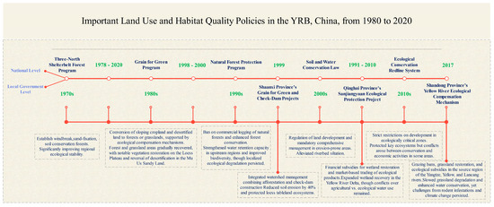
Figure 17.
Important land use and habitat quality policies in the YRB, China, from 1980 to 2020.
To address persistent habitat quality challenges and enhance the ecological resilience in the Yellow River Basin, the following prioritized strategies are proposed:
- (1)
- Cross-Provincial Ecological Compensation: Align market incentives with conservation priorities in critical ecological zones like riparian corridors and headwaters, fostering interregional equity through compensation mechanisms;
- (2)
- Geomorphic Threshold-Based Zoning: Prohibit industrial activities in vulnerable areas while allowing sustainable agroforestry in transitional landscapes, balancing protection and development;
- (3)
- Integrated Basin Governance: Coordinate upstream–downstream responsibilities to prioritize sediment control, groundwater recharge, and wetland restoration, ensuring ecological resilience across scales. These strategies aim to reconcile historical policy imbalances by addressing scale mismatches and economic–ecological trade-offs and monitoring gaps, thereby fostering sustainable habitat quality trajectories across the basin.
4.5. Limitations of This Study
This study focuses on the analysis of spatial and temporal patterns and driving factors of land use change, but this research still has several limitations. This study mainly focuses on ecological indicators, meteorological elements, and explicit economic indicators, while the land use change was jointly influenced by a diverse range of factors [79,80,81], and the integrated impacts of climate change, extreme events, and drought stress can be considered comprehensively and be integrated in future studies to comprehensively explain the mechanism of land use change. In future research, the acquisition of high-precision data [82,83], the optimization of model parameterization, and validation methods could be strengthened to improve the understanding and prediction of LUCC and different ecosystems. Meanwhile, homogenization is observed in the HQACI, which may be attributed to the vast spatial scale of the YRB. Future research should focus on smaller-scale regions to better elucidate the relationship between the habitat quality and spatial autocorrelation.
5. Conclusions
This study systematically analyzes the evolution pattern of the land use pattern and its driving mechanism in the Yellow River Basin from 1980 to 2020 and has simulated the land use scenarios under different policy orientations in 2040, and the main conclusions are as follows: The YRB has exhibited a trend of the ecological transformation of farmland and unutilized land to forest and grassland (increased by 3737.68 km2 and 4521.61 km2, respectively), and the construction land expansion (+12,941.77 km2) has been highly coupled with the urbanization process. Spatially, the Loess Plateau region has the significant effect of forest and grassland restoration, and the downstream provinces of Henan and Shandong have become hotspots for construction land expansion. Changes in farmland were dominated by both the population and economy, and the forest and grassland restoration was driven by the synergy of ecological engineering and climatic factors, while the expansion of construction land reflected the cohesion of the population concentration. The double-factor interaction revealed the nonlinear enhancement effect of the ecological and natural elements on the evolution of the land system, highlighting the coupling mechanism of the natural and humanity elements. The share of forest and grassland increases to 50.35% (+12.94%) in the ecological protection scenario, and the expansion of construction land reaches 21.57% (+13.84%) in the economic development scenario. The persistently high proportion of unused land (>3.61%) in Inner Mongolia reveals ecological vulnerability. The contradiction between the farmland and construction land in the midstream and downstream provinces has intensified, and differentiated control strategies will be required.
Under 2020 conditions, the habitat quality exhibits a marked spatial polarization, with high-quality clusters concentrated in riparian corridors and mid-elevation plateaus, while low-quality zones dominate agricultural plains and arid margins. Scenario projections highlight divergent pathways: the ecological protection scenario retains high-quality clusters and reduces low-quality coverage, demonstrating a targeted conservation efficacy, particularly along major tributaries. Conversely, the economic development scenario amplifies spatial fragmentation, with low-quality zones expanding in industrializing regions and high–low (H-L) outliers surging near urban peripheries, reflecting the abrupt habitat degradation at development frontiers. The natural development scenario mirrors these fragmentation trends, underscoring systemic pressures from unregulated land use transitions.
The HQACI quantifies the declining spatial synergy across all scenarios (2020: 0.373; 2040: 0.345–0.349), signaling ecological homogenization, which is characterized by the habitat quality becoming uniformly distributed at lower resilience levels. This homogenization stems from overlapping drivers: aridification in upstream regions, groundwater depletion in agricultural hubs, and coastal urbanization downstream. Strategic priorities must therefore balance connectivity and regulation through three approaches: (1) preserving high-quality riparian corridors, (2) implementing gradient restoration in transitional ecotones, and (3) enforcing dynamic zoning to mitigate edge effects. These measures, informed by scale-dependent clustering thresholds, could counteract fragmentation while accommodating the basin’s dual role as an ecological refuge and economic engine.
Author Contributions
Conceptualization, X.Z. and C.Z.; methodology, X.Z. and F.R.; data curation, X.Z. and J.L.; visualization, X.Z. and J.L.; writing—original draft, X.Z. and J.L.; writing—review and editing, X.Z., Z.Z. and X.H.; supervision, C.Z. All authors have read and agreed to the published version of the manuscript.
Funding
This study was supported by The General Program of National Natural Science Foundation of China, grant number 42371208.
Institutional Review Board Statement
Not applicable.
Data Availability Statement
The original contributions presented in the study are included in the article; further inquiries can be directed to the corresponding author.
Conflicts of Interest
The authors declare no conflicts of interest.
References
- IPCC. Climate Change 2021: The Physical Science Basis; Contribution of Working Group I to the Sixth Assessment Report of the Intergovernmental Panel on Climate Change; Cambridge University Press: Cambridge, UK, 2021. [Google Scholar]
- Tian, F.; Liu, L.-Z.; Yang, J.-H.; Wu, J.-J. Vegetation greening in more than 94% of the Yellow River Basin (YRB) region in China during the 21st century caused jointly by warming and anthropogenic activities. Ecol. Indic. 2021, 125, 107479. [Google Scholar] [CrossRef]
- Liu, J.; Zhang, Z.; Xu, X.; Kuang, W.; Zhou, W.; Zhang, S.; Li, R.; Yan, C.; Yu, D.; Wu, S.; et al. Spatial Patterns and Driving Forces of Land Use Change in China in the Early 21st Century. Acta Geogr. Sin. 2009, 64, 1411–1420. [Google Scholar] [CrossRef]
- Li, T.; Zhang, Q.; Wang, G.; Singh, V.P.; Zhao, J.; Sun, S.; Wang, D.; Liu, T.; Duan, L. Ecological degradation in the Inner Mongolia reach of the Yellow River Basin, China: Spatiotemporal patterns and driving factors. Ecol. Indic. 2023, 154, 110498. [Google Scholar] [CrossRef]
- NASA. Human Activity in China and India Dominates the Greening of Earth, NASA Study Shows. Available online: https://www.nasa.gov/feature/ames/human-activity-in-china-and-india-dominates-the-greening-of-earth-nasa-study-shows (accessed on 12 February 2019).
- Piao, S.; Wang, X.; Park, T.; Chen, C.; Lian, X.; He, Y.; Bjerke, J.W.; Chen, A.; Ciais, P.; Tømmervik, H.; et al. Characteristics, drivers and feedbacks of global greening. Nat. Rev. Earth Environ. 2020, 1, 14–27. [Google Scholar] [CrossRef]
- Yang, Y.; Roderick, M.L.; Guo, H.; Miralles, D.G.; Zhang, L.; Fatichi, S.; Luo, X.; Zhang, Y.; McVicar, T.R.; Tu, Z.; et al. Evapotranspiration on a greening Earth. Nat. Rev. Earth Environ. 2023, 4, 626–641. [Google Scholar] [CrossRef]
- Gou, Y.; Tao, Y.; Kou, P.; Alonso, A.; Luo, X.; Tian, H. Elucidate the complex drivers of significant greening on the Loess Plateau from 2000 to 2020. Environ. Dev. 2024, 50, 100991. [Google Scholar] [CrossRef]
- Ji, X.; Sun, Y.; Guo, W.; Zhao, C.; Li, K. Land use and habitat quality change in the Yellow River Basin: A perspective with different CMIP6-based scenarios and multiple scales. J. Environ. Manag. 2023, 345, 14. [Google Scholar] [CrossRef]
- Li, J.; Xi, M.; Wang, L.; Li, N.; Wang, H.; Qin, F. Vegetation Responses to Climate Change and Anthropogenic Activity in China, 1982 to 2018. Int. J. Environ. Res. Public Health 2022, 19, 7391. [Google Scholar] [CrossRef]
- Zhou, G.; Long, H. Explanation of land-use system evolution: Modes, trends, and mechanisms. Land Use Policy 2025, 150, 107470. [Google Scholar] [CrossRef]
- Zhou, J.; Yang, J.; Tang, Z.; Xue, L.; Zhang, W.; Zhang, J. Driving mechanisms of ecosystem services and their trade-offs and synergies in the transition zone between the Qinghai-Tibet Plateau and the Loess Plateau. Ecol. Indic. 2025, 171, 113148. [Google Scholar] [CrossRef]
- Nyland, K.E.; Gunn, G.E.; Shiklomanov, N.I.; Engstrom, R.N.; Streletskiy, D.A. Land Cover Change in the Lower Yenisei River Using Dense Stacking of Landsat Imagery in Google Earth Engine. Remote Sens. 2018, 10, 1226. [Google Scholar] [CrossRef]
- Kindu, M.; Schneider, T.; Teketay, D.; Knoke, T. Drivers of land use/land cover changes in Munessa-Shashemene landscape of the south-central highlands of Ethiopia. Environ. Monit. Assess. 2015, 187, 1–17. [Google Scholar] [CrossRef] [PubMed]
- Kou, P.; Xu, Q.; Jin, Z.; Yunus, A.P.; Luo, X.; Liu, M. Complex anthropogenic interaction on vegetation greening in the Chinese Loess Plateau. Sci. Total Environ. 2021, 778, 146065. [Google Scholar] [CrossRef] [PubMed]
- Lin, X.; Jiao, X.; Tian, Z.; Sun, Q.; Zhang, Y.; Zhang, P.; Ji, Z.; Chen, L.; Lun, F.; Chang, X.; et al. Projecting Diversity Conflicts of Future Land System Pathways in China Under Anthropogenic and Climate Forcing. Earth’s Future 2023, 11, e2022EF003406. [Google Scholar] [CrossRef]
- Winkler, K.; Fuchs, R.; Rounsevell, M.; Herold, M. Global land use changes are four times greater than previously estimated. Nat. Commun. 2021, 12, 2501. [Google Scholar] [CrossRef]
- Chen, S.; Yan, J.; Wang, Y.; Chang, Z.; Yu, G.; Li, J.; Jiang, J.; Wang, L.; Zhang, S.; Chen, Y.; et al. Analysis of Spatio-Temporal Relationship Between Ecosystem Services and Human Footprints Under Different Human Activity Gradients: A Case Study of Xiangjiang River Basin. Remote Sens. 2024, 16, 4212. [Google Scholar] [CrossRef]
- Li, Y.; Qin, Y.; Rong, P. Evolution of potential evapotranspiration and its sensitivity to climate change based on the Thornthwaite, Hargreaves, and Penman–Monteith equation in environmental sensitive areas of China. Atmos. Res. 2022, 273, 106178. [Google Scholar] [CrossRef]
- Qian, L.; Yu, X.; Wu, L.; Zhang, Z.; Fan, S.; Du, R.; Liu, X.; Yang, Q.; Qiu, R.; Cui, Y.; et al. Improving high uncertainty of evapotranspiration products under extreme climatic conditions based on deep learning and ERA5 reanalysis data. J. Hydrol. 2024, 641, 131755. [Google Scholar] [CrossRef]
- Chen, J.; Liu, M.; Chen, X.; Li, Z. Spatio-temporal evolution, driving mechanisms, and simulation of land use and cover in China from 2000 to 2060. Appl. Spat. Anal. Policy 2024, 17, 1631–1652. [Google Scholar] [CrossRef]
- Li, X.; Chen, Y. Projecting the future impacts of China’s cropland balance policy on ecosystem services under the shared socioeconomic pathways. J. Clean. Prod. 2020, 250, 119489. [Google Scholar] [CrossRef]
- Xu, D.; Yu, C.; Lin, W.; Yao, J.; Zhou, W. Spatiotemporal Evolution and Prediction of Land Use and Carbon Stock in Shanghai. Land 2024, 13, 267. [Google Scholar] [CrossRef]
- Zhao, X.; Miao, C. Spatial-Temporal Changes and Simulation of Land Use in Metropolitan Areas: A Case of the Zhengzhou Metropolitan Area, China. Int. J. Environ. Res. Public Health 2022, 19, 14089. [Google Scholar] [CrossRef] [PubMed]
- Yang, Y.; Yu, C.; Liu, M.; Wei, H. Uncovering the coupling relationships and key factors linking ecosystem services to human well-being through system dynamics: A case study in the Qinghai-Tibet Plateau. Ecol. Indic. 2024, 166, 112408. [Google Scholar] [CrossRef]
- Ouyang, Z.; Zheng, H.; Xiao, Y.; Polasky, S.; Daily, G.C. Improvements in ecosystem services from investments in natural capital. Science 2016, 352, 1455–1459. [Google Scholar] [CrossRef]
- Kuang, X.X.; Jiao, J.J. Review on climate change on the Tibetan Plateau during the last half century. J. Geophys. Res.-Atmos. 2016, 121, 3979–4007. [Google Scholar] [CrossRef]
- Xiao, J.; Zhang, Y.; Xu, H. Response of ecosystem service values to land use change, 2002–2021. Ecol. Indic. 2024, 160, 111947. [Google Scholar] [CrossRef]
- Zou, Z.; Yuan, X.; Zhang, Z.; Li, X.; Zhou, C. Spatiotemporal Evolution and Influencing Factors of Coupling and Coordination between the Ecosystem Service Value and Economy in the Pearl River Delta Urban Agglomeration of China. Land 2024, 13, 1670. [Google Scholar] [CrossRef]
- Sang, L.; Zhang, C.; Yang, J.; Zhu, D.; Yun, W. Simulation of land use spatial pattern of towns and villages based on CA–Markov model. Math. Comput. Model. 2011, 54, 938–943. [Google Scholar] [CrossRef]
- Zhang, M.; Chen, E.; Zhang, C.; Liu, C.; Li, J. Multi-scenario simulation of land use change and ecosystem service value based on the markov–FLUS model in Ezhou city, China. Sustainability 2024, 16, 6237. [Google Scholar] [CrossRef]
- Chen, Y.Q.; Zhang, F.Y.; Lin, J.Y. Projecting Future Land Use Evolution and Its Effect on Spatiotemporal Patterns of Habitat Quality in China. Appl. Sci. 2025, 15, 1042. [Google Scholar] [CrossRef]
- Chen, Y.L.; He, Z.L.; Yue, T.M.; Mu, W.C.; Qin, F. Spatiotemporal evolution and multi-scenario prediction of habitat quality in the Yellow River Basin. Front. Ecol. Evol. 2023, 11, 1226676. [Google Scholar] [CrossRef]
- Wang, X.; Liu, B.; Chen, J.Z.; Arash, M.; Zhang, B.; Chang, Q.; Liu, J.; You, W.X. Assessing the impact of land use change on habitat quality in Zhongwei through multiscenario simulation using the PLUS and InVEST models. Sci. Rep. 2025, 15, 12355. [Google Scholar] [CrossRef] [PubMed]
- Meng, R.; Cai, J.; Xin, H.; Meng, Z.; Dang, X.; Han, Y. Spatio-Temporal Changes in Land Use and Habitat Quality of Hobq Desert along the Yellow River Section. Int. J. Environ. Res. Public Health 2023, 20, 3599. [Google Scholar] [CrossRef]
- Li, Y.; Xie, Z.; Qin, Y.; Zheng, Z. Estimating Relations of Vegetation, Climate Change, and Human Activity: A Case Study in the 400 mm Annual Precipitation Fluctuation Zone, China. Remote Sens. 2019, 11, 1159. [Google Scholar] [CrossRef]
- Li, J.; Xi, M.; Pan, Z.; Liu, Z.; He, Z.; Qin, F. Response of NDVI and SIF to Meteorological Drought in the Yellow River Basin from 2001 to 2020. Water 2022, 14, 2978. [Google Scholar] [CrossRef]
- Li, J.; Qin, F.; Wang, Y.; Zhao, X.; Yu, M.; Chen, S.; Jiang, J.; Wang, L.; Yan, J. Spatiotemporal Variation of Water Use Efficiency and Its Responses to Climate Change in the Yellow River Basin from 1982 to 2018. Remote Sens. 2025, 17, 316. [Google Scholar] [CrossRef]
- Guo, X.; Zhang, H.; Wu, Z.; Zhao, J.; Zhang, Z. Comparison and Evaluation of Annual NDVI Time Series in China Derived from the NOAA AVHRR LTDR and Terra MODIS MOD13C1 Products. Sensors 2017, 17, 1298. [Google Scholar] [CrossRef]
- Chen, T.; Tang, G.; Yuan, Y.; Guo, H.; Xu, Z.; Jiang, G.; Chen, X. Unraveling the relative impacts of climate change and human activities on grassland productivity in Central Asia over last three decades. Sci. Total Environ. 2020, 743, 140649. [Google Scholar] [CrossRef]
- Zhang, Y.; Jiang, X.; Lei, Y.; Gao, S. The contributions of natural and anthropogenic factors to NDVI variations on the Loess Plateau in China during 2000–2020. Ecol. Indic. 2022, 143, 109342. [Google Scholar] [CrossRef]
- Zhang, X.Y.; Liu, K.; Li, X.K.; Wang, S.D.; Wang, J.N.A. Vulnerability assessment and its driving forces in terms of NDVI and GPP over the Loess Plateau, China. Phys. Chem. Earth 2022, 125, 103106. [Google Scholar] [CrossRef]
- Ru, X.; Qiao, L.; Zhang, H.; Bai, T.; Min, R.; Wang, Y.; Wang, Q.; Song, H. Effects of land use and land cover change under shared socioeconomic pathways on future climate in the Yellow River basin, China. Urban Clim. 2024, 55, 101867. [Google Scholar] [CrossRef]
- Wang, H.; Qin, F.; Xu, C.; Li, B.; Guo, L.; Wang, Z. Evaluating the suitability of urban development land with a Geodetector. Ecol. Indic. 2021, 123, 107339. [Google Scholar] [CrossRef]
- Hamad, R.; Balzter, H.; Kolo, K. Predicting land use/land cover changes using a CA-Markov model under two different scenarios. Sustainability 2018, 10, 3421. [Google Scholar] [CrossRef]
- Subedi, P.; Subedi, K.; Thapa, B. Application of a hybrid cellular automaton–Markov (CA-Markov) model in land-use change prediction: A case study of Saddle Creek Drainage Basin, Florida. Appl. Ecol. Environ. Sci. 2013, 1, 126–132. [Google Scholar] [CrossRef]
- Liang, X.; Guan, Q.; Clarke, K.C.; Liu, S.; Wang, B.; Yao, Y. Understanding the drivers of sustainable land expansion using a patch-generating land use simulation (PLUS) model: A case study in Wuhan, China. Comput. Environ. Urban Syst. 2021, 85, 101569. [Google Scholar] [CrossRef]
- Xu, L.; Liu, X.; Tong, D.; Liu, Z.; Yin, L.; Zheng, W. Forecasting urban land use change based on cellular automata and the PLUS model. Land 2022, 11, 652. [Google Scholar] [CrossRef]
- Feng, Z.; Zhang, P. “Grain for Green” Policy and Its Impacts on Grain Supply in West China. In China’s West Region Development; The University of Chicago Press: Chicago, IL, USA, 2004; pp. 291–307. [Google Scholar]
- Liu, Y.; Yuan, L. Evolution of water-use efficiency in the Yangtze River Economic Belt based on national strategies and water environment treatment. Ecol. Inform. 2022, 69, 101642. [Google Scholar] [CrossRef]
- Niu, H.; Xiu, Z.; Xiao, D. Impact of land-use change on ecological vulnerability in the Yellow River Basin based on a complex network model. Ecol. Indic. 2024, 166, 112212. [Google Scholar] [CrossRef]
- Yang, R.; Chen, H.; Chen, S.; Ye, Y. Spatiotemporal evolution and prediction of land use/land cover changes and ecosystem service variation in the Yellow River Basin, China. Ecol. Indic. 2022, 145, 109579. [Google Scholar] [CrossRef]
- Zhao, X.; Miao, C. Research on the Spatial Pattern of the Logistics Industry Based on POI Data: A Case Study of Zhengzhou City. Sustainability 2023, 15, 15574. [Google Scholar] [CrossRef]
- Yang, H.; Zhong, X.; Deng, S.; Nie, S. Impact of LUCC on landscape pattern in the Yangtze River Basin during 2001–2019. Ecol. Inform. 2022, 69, 101631. [Google Scholar] [CrossRef]
- Rodrigo-Comino, J.; Cambronero, L.; Gonzalez-Moreno, M.T.; Keesstra, S.D.; Vivar, J.G.; Cerda, A.; Senciales, J.M. Chapter 2—Sustainable development and integrated soil management: Tools and keys for surveying the landscape evolution and degradation processes in Mediterranean mountainous regions. In Environmental Sustainability and Global Change; Salvati, L., Ed.; Elsevier: London, UK, 2025; pp. 19–31. [Google Scholar]
- Du, L.; Dong, C.; Kang, X.; Qian, X.; Gu, L. Spatiotemporal evolution of land cover changes and landscape ecological risk assessment in the Yellow River Basin, 2015–2020. J. Environ. Manag. 2023, 332, 117149. [Google Scholar] [CrossRef] [PubMed]
- Song, Y.; Wang, M.; Sun, X.; Fan, Z. Quantitative assessment of the habitat quality dynamics in Yellow River Basin, China. Environ. Monit. Assess. 2021, 193, 614. [Google Scholar] [CrossRef] [PubMed]
- An, X. Responses of Water Use Efficiency to climate change in evapotranspiration and transpiration ecosystems. Ecol. Indic. 2022, 141, 109157. [Google Scholar] [CrossRef]
- Cai, L.; Fan, D.; Wen, X.; Wang, H.; Badarifu; Wang, S. Spatiotemporal tendency of agricultural water use efficiency in the northernmost Yellow River: Indicator comparison and interactive driving factors. J. Arid Environ. 2022, 205, 104822. [Google Scholar] [CrossRef]
- Du, Q.; Sun, Y.; Guan, Q.; Pan, N.; Wang, Q.; Ma, Y.; Li, H.; Liang, L. Vulnerability of grassland ecosystems to climate change in the Qilian Mountains, northwest China. J. Hydrol. 2022, 612, 128305. [Google Scholar] [CrossRef]
- Li, F.; Wu, S.; Liu, H.; Yan, D. Biodiversity loss through cropland displacement for urban expansion in China. Sci. Total Environ. 2024, 907, 167988. [Google Scholar] [CrossRef]
- Xu, Y.; Lu, Y.-G.; Zou, B.; Xu, M.; Feng, Y.-X. Unraveling the enigma of NPP variation in Chinese vegetation ecosystems: The interplay of climate change and land use change. Sci. Total Environ. 2024, 912, 169023. [Google Scholar] [CrossRef]
- Zhang, L.; Deng, C.; Kang, R.; Yin, H.; Xu, T.; Kaufmann, H.J. Assessing the responses of ecosystem patterns, structures and functions to drought under climate change in the Yellow River Basin, China. Sci. Total Environ. 2024, 929, 172603. [Google Scholar] [CrossRef]
- Zhang, S.; Yang, D.; Jayawardena, A.W.; Xu, X.; Yang, H. Hydrological change driven by human activities and climate variation and its spatial variability in Huaihe Basin, China. Hydrol. Sci. J. 2016, 61, 1370–1382. [Google Scholar] [CrossRef]
- Hao, Z.C.; Singh, V.P. Drought characterization from a multivariate perspective: A review. J. Hydrol. 2015, 527, 668–678. [Google Scholar] [CrossRef]
- Liu, L.Z.; Yang, X.; Zhou, H.K.; Liu, S.S.; Zhou, L.; Li, X.H.; Yang, J.H.; Han, X.Y.; Wu, J.J. Evaluating the utility of solar-induced chlorophyll fluorescence for drought monitoring by comparison with NDVI derived from wheat canopy. Sci. Total Environ. 2018, 625, 1208–1217. [Google Scholar] [CrossRef] [PubMed]
- Deng, G.; Jiang, H.; Zhu, S.; Wen, Y.; He, C.; Wang, X.; Sheng, L.; Guo, Y.; Cao, Y. Projecting the response of ecological risk to land use/land cover change in ecologically fragile regions. Sci. Total Environ. 2024, 914, 169908. [Google Scholar] [CrossRef]
- Ji, R.; Wang, C.; Wang, P.; Wang, W.; Chen, N. Quantitative analysis of spatiotemporal disparity of urban water use efficiency and its driving factors in the Yangtze River Economic Belt, China. J. Hydrol. Reg. Stud. 2024, 51, 101647. [Google Scholar] [CrossRef]
- Ren, D.-F.; Cao, A.-H.; Wang, F.-Y. Response and Multi-Scenario Prediction of Carbon Storage and Habitat Quality to Land Use in Liaoning Province, China. Sustainability 2023, 15, 4500. [Google Scholar] [CrossRef]
- Liu, X.; Lai, Q.; Yin, S.; Bao, Y.; Tong, S.; Adiya, Z.; Sanjjav, A.; Gao, R. Spatio-temporal patterns and control mechanism of the ecosystem carbon use efficiency across the Mongolian Plateau. Sci. Total Environ. 2024, 907, 167883. [Google Scholar] [CrossRef]
- Tian, J.; Feng, C.; Fu, G.; Fan, L.; Wang, W. Contribution of different types of terrestrial protected areas to carbon sequestration services in China: 1980–2020. Front. Ecol. Evol. 2023, 11, 1074410. [Google Scholar] [CrossRef]
- Liu, Q.; Gan, L.; Wu, J.; Zhou, J.; Li, S.; Wu, H.; Wang, B.; Liang, L.; Yan, D. Deviation of hydrological regimes caused by blockage of hydrological connectivity: Implications for wetland restoration and management. CATENA 2025, 255, 109025. [Google Scholar] [CrossRef]
- Rinaldo, A.; Rodriguez-Iturbe, I. Ecohydrology 2.0. Rend. Lincei. Sci. Fis. Nat. 2022, 33, 245–270. [Google Scholar] [CrossRef]
- Shi, F.; Liu, S.; An, Y.; Sun, Y.; Zhao, S.; Liu, Y.; Li, M. Spatio-Temporal Dynamics of Landscape Connectivity and Ecological Network Construction in Long Yangxia Basin at the Upper Yellow River. Land 2020, 9, 265. [Google Scholar] [CrossRef]
- Rinnan, D.S.; Sica, Y.; Ranipeta, A.; Wilshire, J.; Jetz, W. Multi-scale planning helps resolve global conservation needs with regional priorities. bioRxiv 2021, 2020.2002.2005.936047. [Google Scholar] [CrossRef]
- Wang, S.; Liu, Z.; Chen, Y.; Fang, C. Factors influencing ecosystem services in the Pearl River Delta, China: Spatiotemporal differentiation and varying importance. Resour. Conserv. Recycl. 2021, 168, 105477. [Google Scholar] [CrossRef]
- Rahman, I.U.; Afzal, A.; Iqbal, Z.; Hashem, A.; Al-Arjani, A.-B.F.; Alqarawi, A.A.; Abd_Allah, E.F.; Abdalla, M.; Calixto, E.S.; Sakhi, S.; et al. Species Distribution Pattern and Their Contribution in Plant Community Assembly in Response to Ecological Gradients of the Ecotonal Zone in the Himalayan Region. Plants 2021, 10, 2372. [Google Scholar] [CrossRef] [PubMed]
- Dahal, K. Peri-urban Development: Discussion with Land Use Zoning, Statutory Provision, and Issues inside Katahari Rural Municipality, Nepal. J. Geogr. Res. 2023, 6, 1–16. [Google Scholar] [CrossRef]
- McDowell, N.G.; Coops, N.C.; Beck, P.S.; Chambers, J.Q.; Gangodagamage, C.; Hicke, J.A.; Huang, C.Y.; Kennedy, R.; Krofcheck, D.J.; Litvak, M.; et al. Global satellite monitoring of climate-induced vegetation disturbances. Trends Plant Sci. 2015, 20, 114–123. [Google Scholar] [CrossRef]
- Naeem, S.; Zhang, Y.; Zhang, X.; Rehman, A.U.; Tang, Z.; Xu, Z.; Li, C.; Azeem, T. Recent change in ecosystem water use efficiency in China mainly dominated by vegetation greening and increased CO2. Remote Sens. Environ. 2023, 298, 113811. [Google Scholar] [CrossRef]
- Yu, L.; Zhao, X.; Gao, X.; Jia, R.; Yang, M.; Yang, X.; Wu, Y.; Siddique, K.H.M. Effect of natural factors and management practices on agricultural water use efficiency under drought: A meta-analysis of global drylands. J. Hydrol. 2021, 594, 125977. [Google Scholar] [CrossRef]
- Chen, S.; Xiong, L.; Ma, Q.; Kim, J.-S.; Chen, J.; Xu, C.-Y. Improving daily spatial precipitation estimates by merging gauge observation with multiple satellite-based precipitation products based on the geographically weighted ridge regression method. J. Hydrol. 2020, 589, 125156. [Google Scholar] [CrossRef]
- Zhang, Y.; Kong, D.; Gan, R.; Chiew, F.H.S.; McVicar, T.R.; Zhang, Q.; Yang, Y. Coupled estimation of 500 m and 8-day resolution global evapotranspiration and gross primary production in 2002–2017. Remote Sens. Environ. 2019, 222, 165–182. [Google Scholar] [CrossRef]


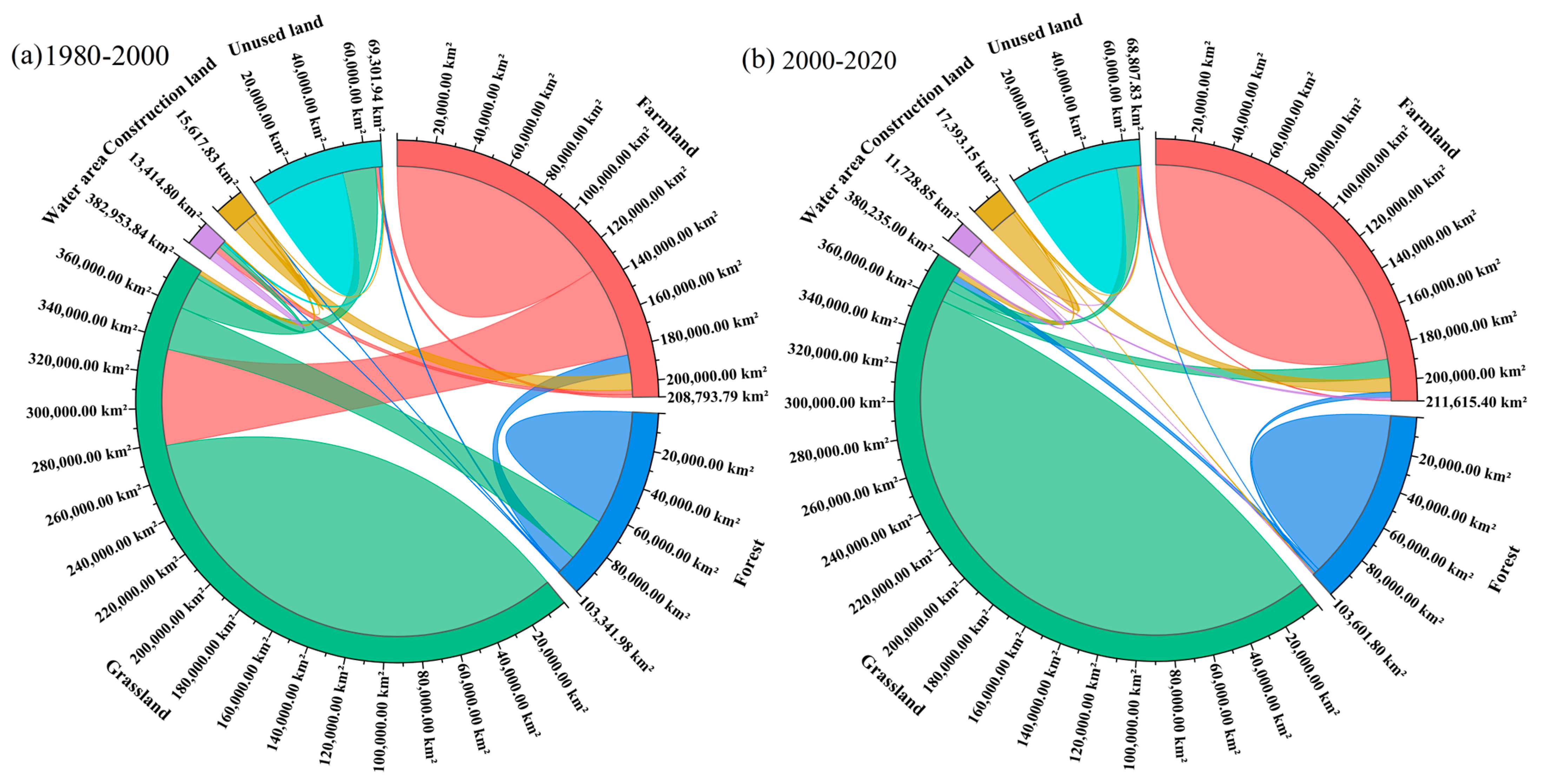

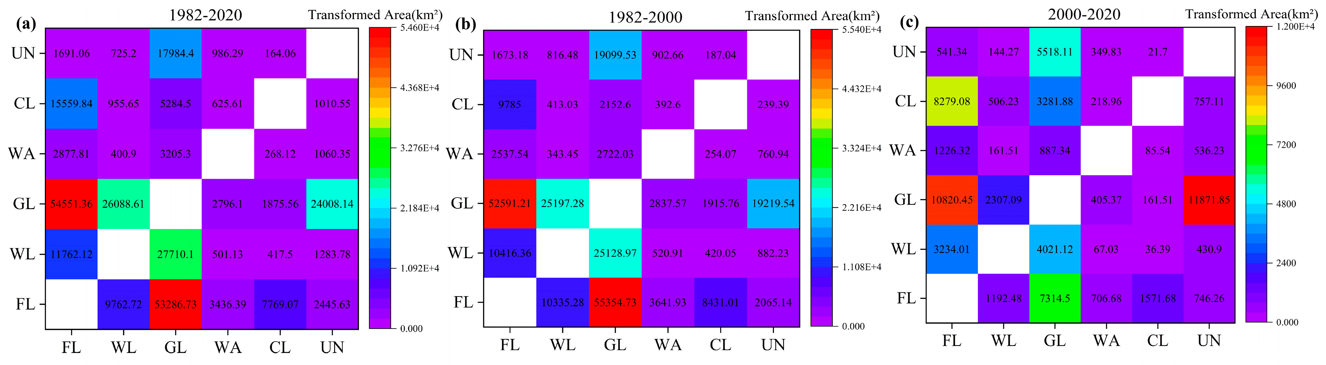
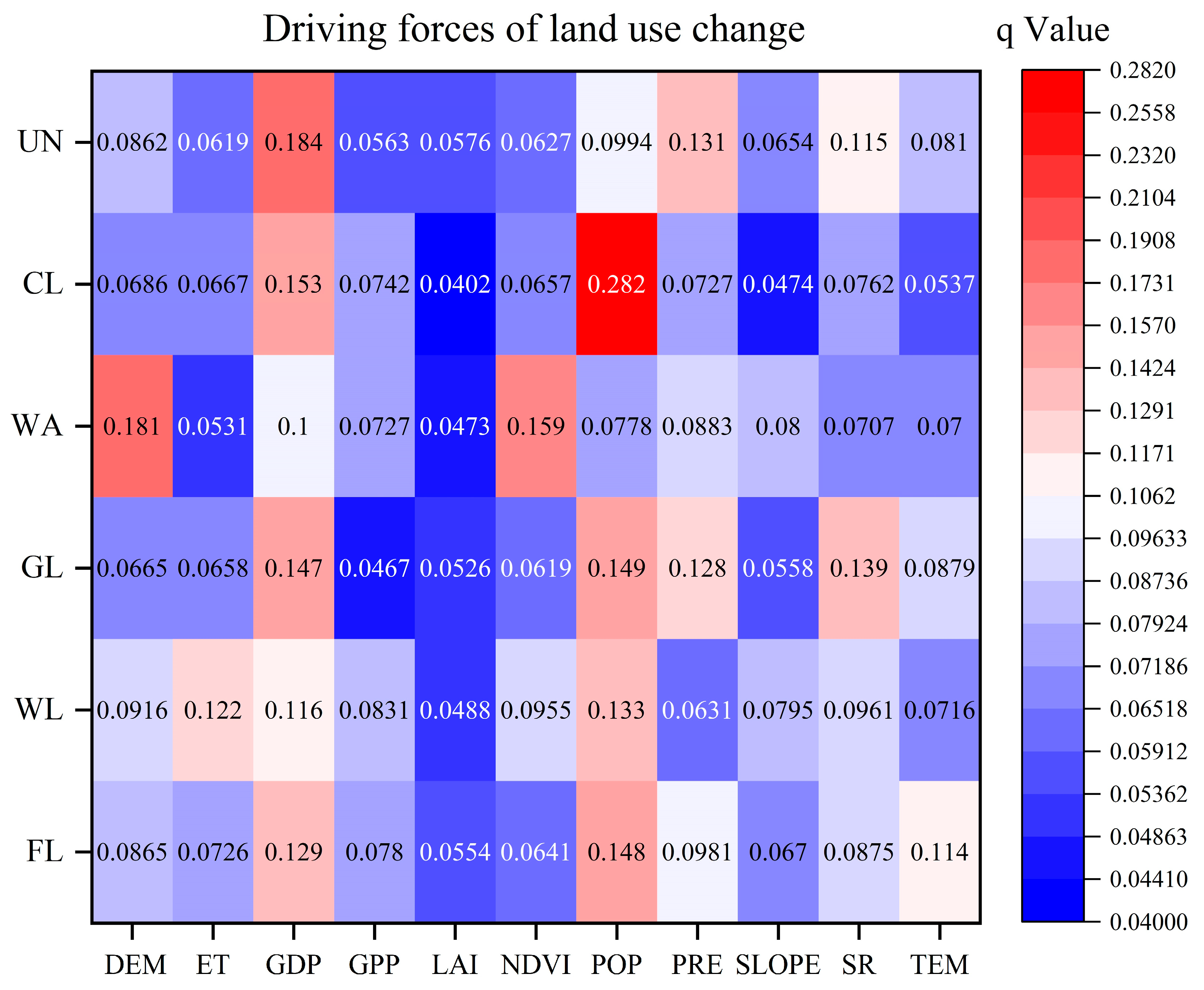

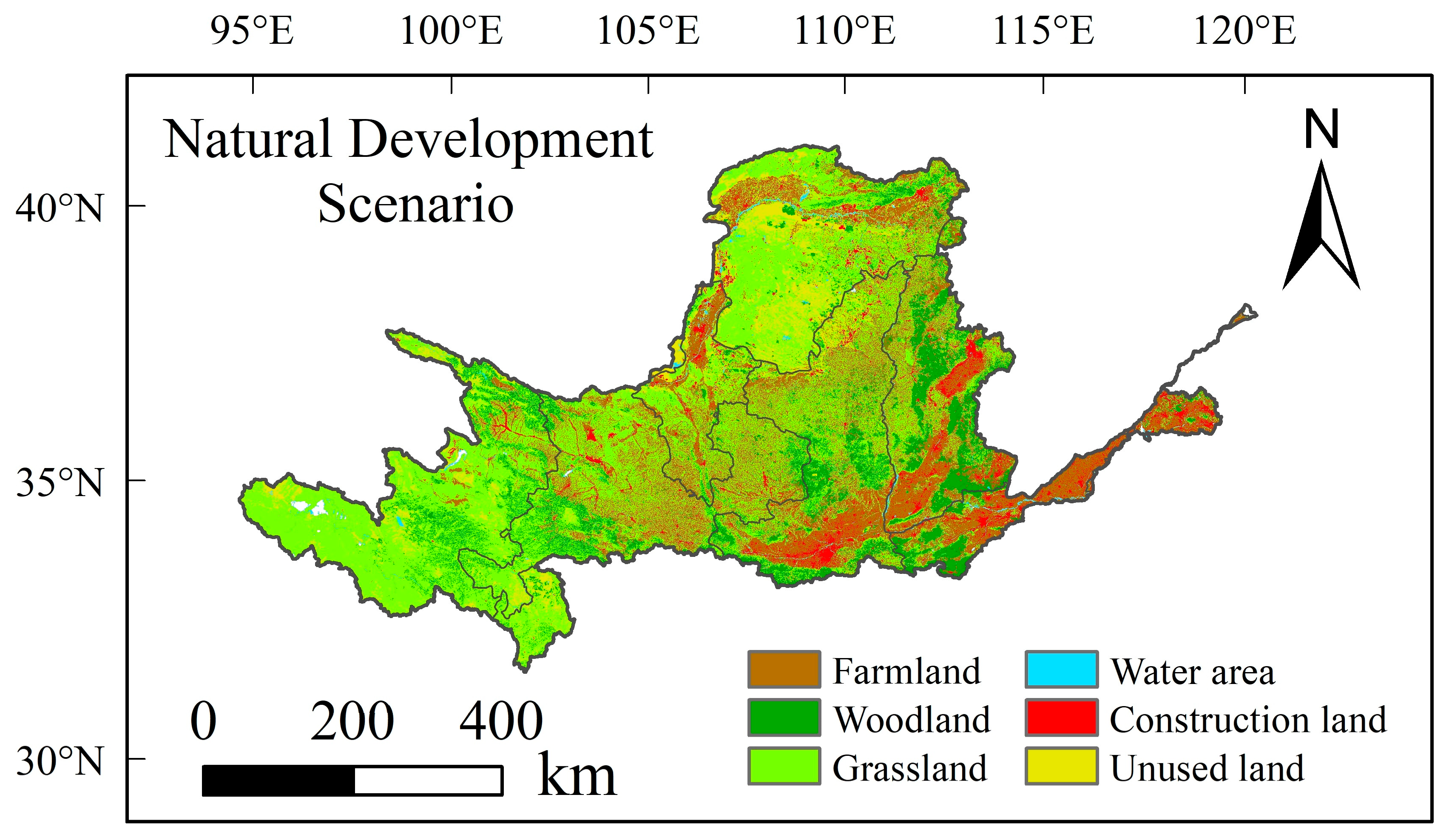
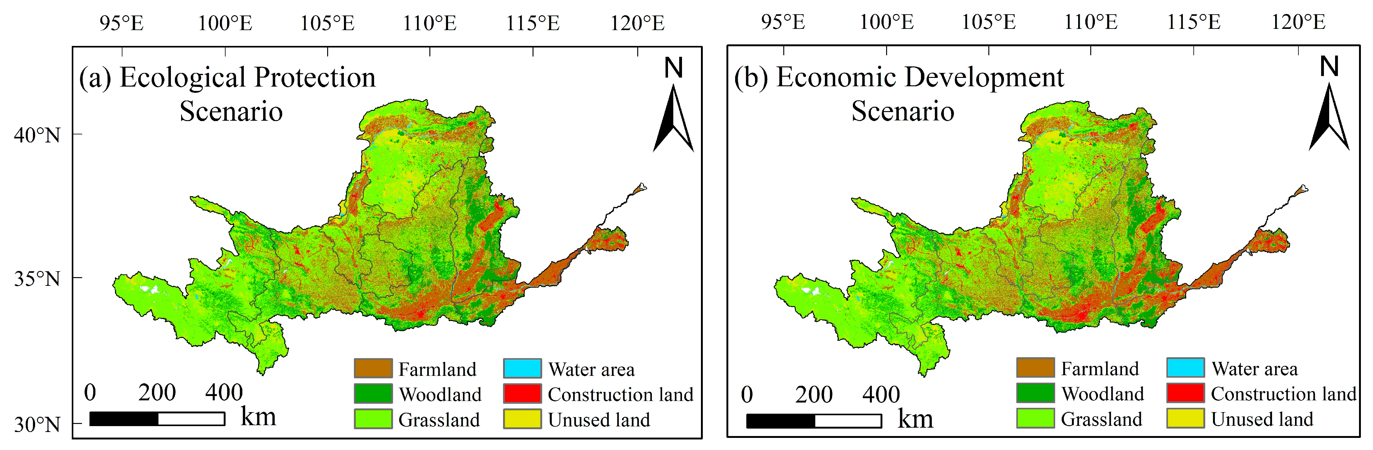
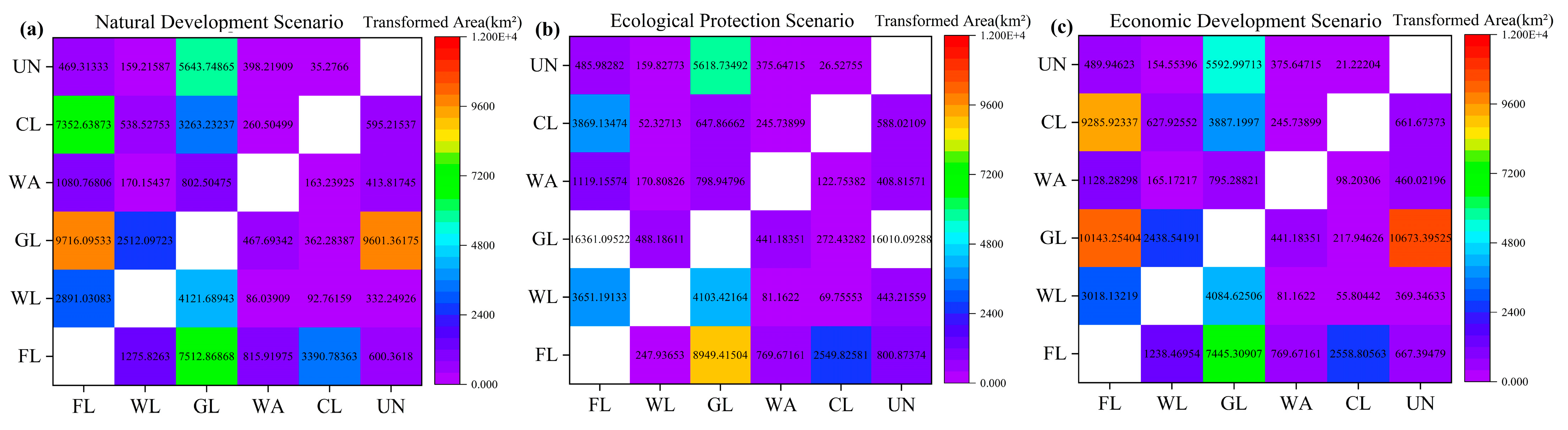
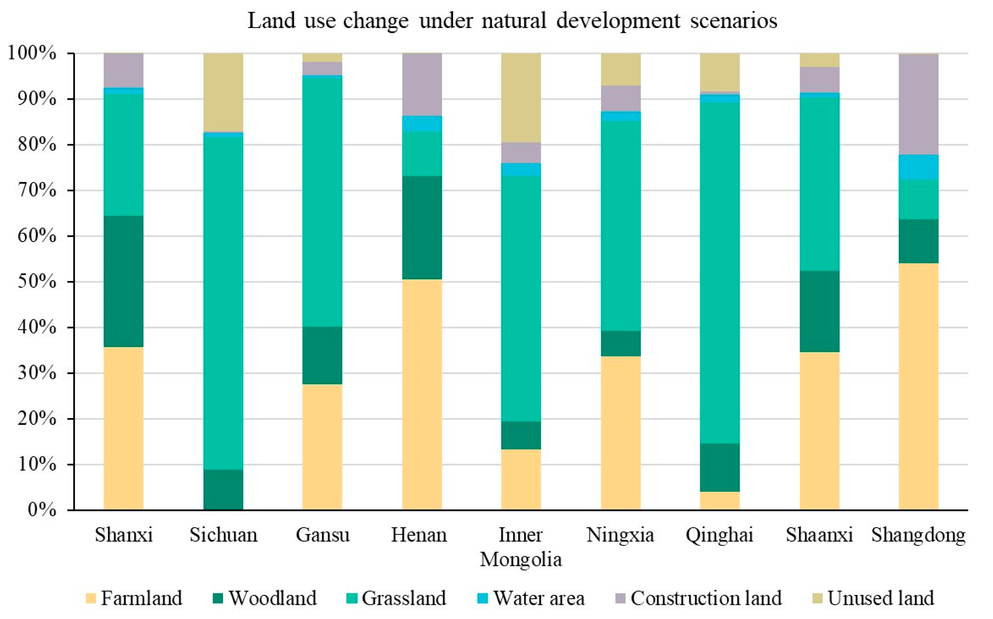
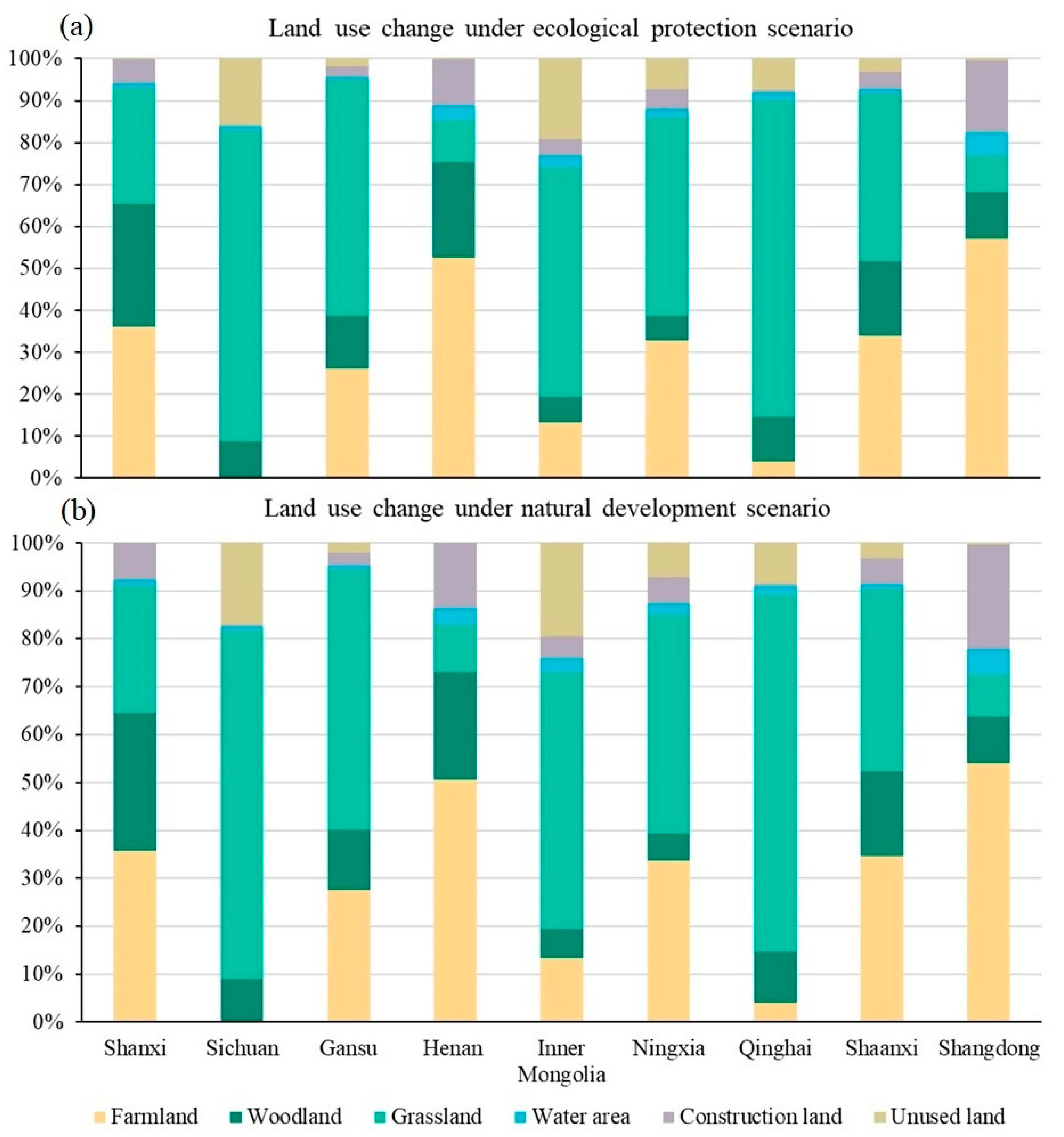
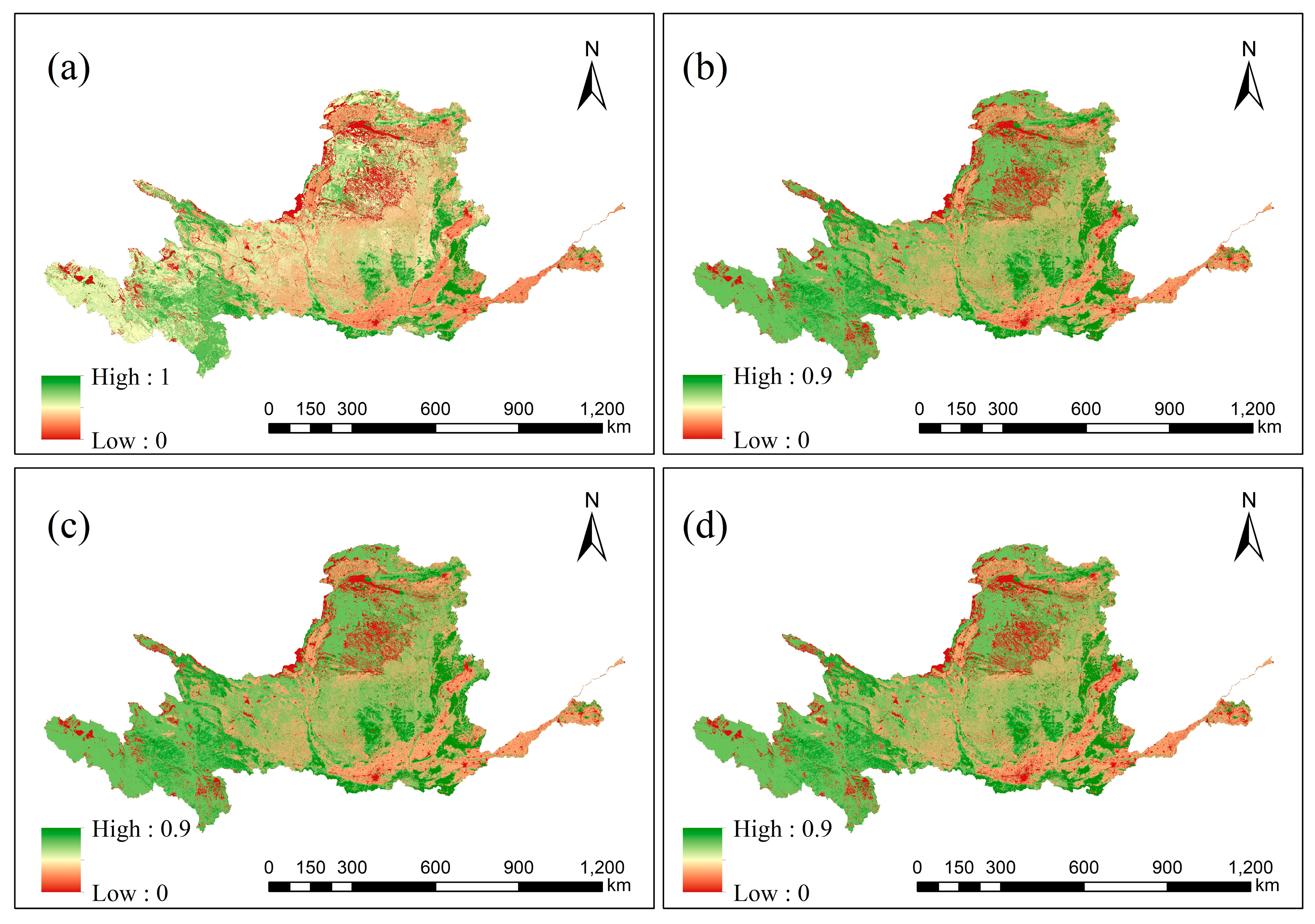
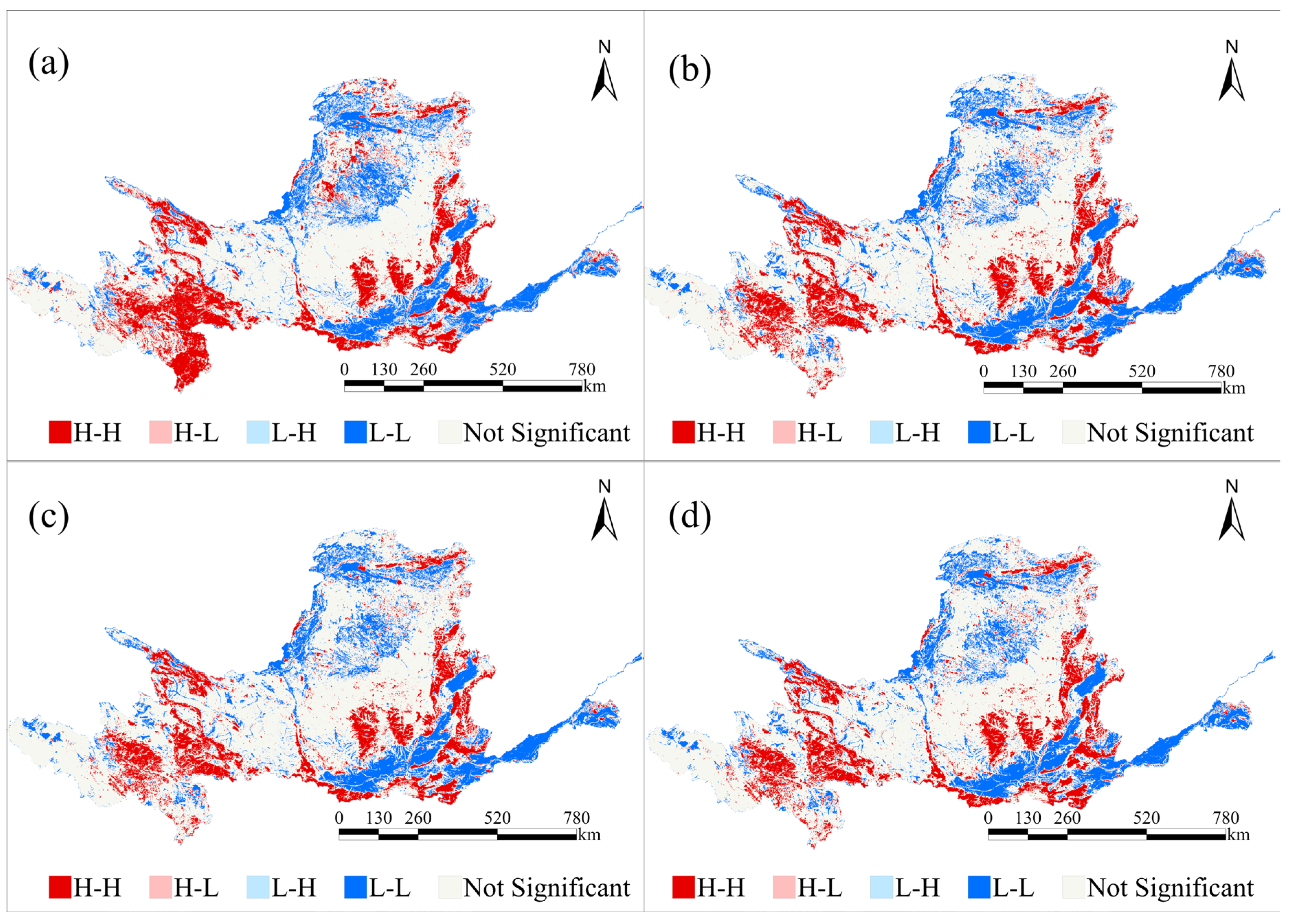

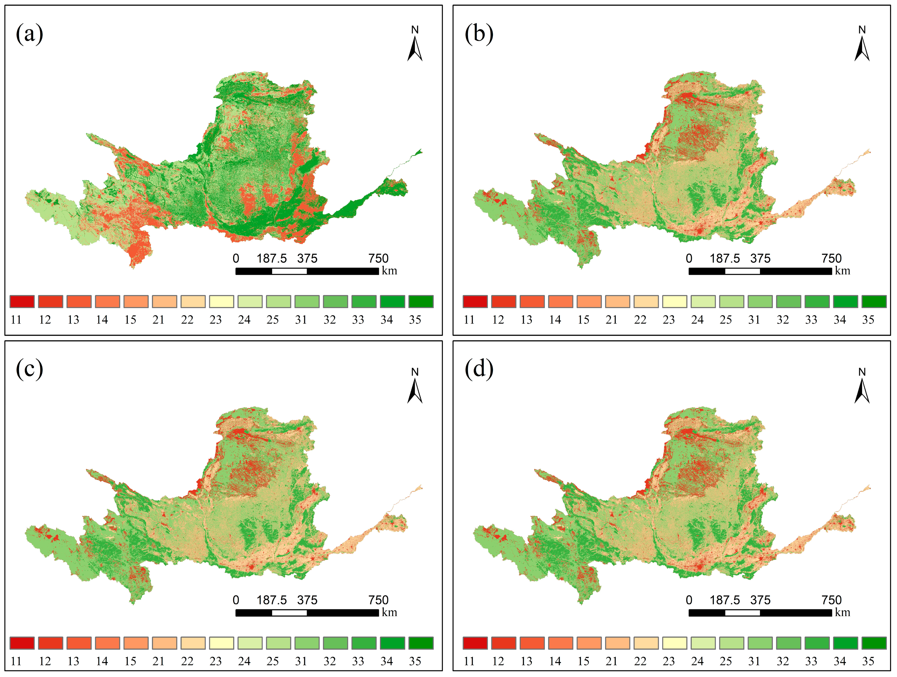

Disclaimer/Publisher’s Note: The statements, opinions and data contained in all publications are solely those of the individual author(s) and contributor(s) and not of MDPI and/or the editor(s). MDPI and/or the editor(s) disclaim responsibility for any injury to people or property resulting from any ideas, methods, instructions or products referred to in the content. |
© 2025 by the authors. Licensee MDPI, Basel, Switzerland. This article is an open access article distributed under the terms and conditions of the Creative Commons Attribution (CC BY) license (https://creativecommons.org/licenses/by/4.0/).