Abstract
Underwater robots require fast and accurate localization results during challenging near-bottom operations. However, commonly used methods such as acoustic baseline localization, dead reckoning, and sensor fusion have limited accuracy. The use of forward-looking sonar (FLS) images to observe the seabed environment for pose estimation has gained significant traction in recent years. This paper proposes a lightweight front-end FLS odometry to provide consistent and accurate localization for underwater robots. The proposed direct FLS odometry (DFLSO) includes several key innovations that realize the extraction of point clouds from FLS images and both image-to-image and image-to-map matching. First, an image processing method is designed to rapidly generate a 3-D point cloud of the seabed using FLS image, enabling pose estimation through point cloud matching. Second, a lightweight keyframe system is designed to construct point cloud submaps, which utilize historical information to enhance global pose consistency and reduce the accumulation of image-matching errors. The proposed odometry algorithm is validated by both simulation experiments and field data from sea trials.
1. Introduction
Underwater robots are essential for executing demanding tasks in harsh seabed conditions, including target search, biological surveys, oceanographic research, seabed exploration and inspection [1], and ocean resource development [2]. These robots require accurate position estimation [3]. Whereas typical acoustic baseline localization approaches perform poorly in time delay and accuracy [4]. Consequently, there is growing interest in leveraging environmental data to enhance underwater localization precision [5], particularly in seabed operations where forward-looking sonar (FLS) images have shown promise in estimating pose transformations [6].
FLS can provide real-time acoustic imaging of areas within a wide aperture in the elevation, azimuth angles and a certain range of distance. FLS can have an azimuth opening angle of approximately 130° and an elevation opening angle of about 30°. The maximum detectable distance can reach nearly 100 m. FLS operates by simultaneously emitting multiple fan-shaped acoustic beams and receiving the echo intensities from different distances in various azimuth directions to form an acoustic image. However, during the process of projecting the 3-D underwater environment into a 2-D image, information about the elevation angle is lost, which introduces ambiguity regarding the actual environment corresponding to the image. Compared with optical cameras, FLS has a significant advantage as it can achieve a much longer imaging distance. Moreover, in contrast to some other sonars, it is capable of real-time imaging at a frequency as high as 15 Hz. Thus, FLS would be highly used for perception and localization.
Recent progress in FLS odometry, however, faces challenges related to the accuracy of relative pose transformations and the accumulation of error. This study introduces algorithmic advancements to improve the precision of pose transformations derived from FLS image matching. Furthermore, a two-stage matching approach is proposed to address the issue of accumulated error in odometry positioning.
Odometry-based positioning methods, widely used in terrestrial applications, estimate self-pose changes using sensor-derived environmental information. Visual odometry (VO) typically matches feature points between adjacent images, while laser odometry (LO) uses 3-D point clouds for matching. In contrast, FLS images present unique challenges: low signal-to-noise ratio (SNR) and resolution, as well as a nonlinear projection model. These challenges arise due to the longer wavelengths of acoustic waves and the similarity in acoustic properties of underwater surfaces [7]. The nonlinear projection of FLS, where pixels represent curved arcs rather than straight rays [8], further complicates the matching process and necessitates specialized techniques for accurate pose estimation. Unlike LiDAR, which directly provides 3-D coordinates, FLS images lack direct point cloud data and lose elevation information during projection. Recovering 3-D information from FLS images before matching could enhance accuracy, drawing inspiration from LO. Thus, developing innovative algorithms for matching adjacent FLS images remains critical to improving the accuracy of relative pose transformations in sonar odometry.
Cumulative errors are inevitably introduced during each image-to-image matching process. Essentially, each matching result contributes to the overall positioning inaccuracy. Relying exclusively on adjacent image matches results in a progressive accumulation of errors with increasing match times. To counteract these cumulative errors, VO commonly employs loop closure detection methods, which identify previously visited locations to correct the estimated trajectory and thereby mitigate long-term drift. On the other hand, LO often utilizes a two-stage approach. In the first stage, initial estimates of relative motion are derived from scan-to-scan matching. During the second stage, the current LiDAR scan is matched against a map constructed from historical data, followed by a scan-to-map registration process. This second stage acts as a global correction, refining the pose obtained from each scan-to-scan match using past environmental information to enhance global pose consistency. This global adjustment effectively diminishes the influence of cumulative errors inherent in LO. Research on loop closure detection using FLS images has achieved some progress; however, there remains a significant gap in the exploration of the two-stage global pose correction method involving image matching with a pre-constructed map. This gap is largely due to the limited research on mapping natural seabed environments using FLS, as it is challenging to rapidly and directly construct past environmental information suitable for matching with current images.
This paper proposes a lightweight front-end FLS odometry solution named Direct FLS Odometry (DFLSO), which is designed to provide fast and accurate positioning for underwater robots. Different from SLAM methods that include loop closure detection and perform global pose optimization after loop closure is detected, this method focuses on improving positioning accuracy and minimizing cumulative errors while ensuring real-time performance, so as to quickly obtain the most accurate pose corresponding to the current FLS image. The DFLSO focuses on enhancing positioning accuracy and minimizing cumulative errors to achieve precise real-time localization. The approach is marked by two core innovations. First, a lightweight FLS image processing technique is developed to efficiently extract elevation information from FLS images, generating a 3-D point cloud suitable for matching to estimate relative poses. Second, a fast keyframe-based submapping approach with overlapping images is designed to create local submaps, directly reducing odometry-based localization errors for each FLS image. The feasibility of the proposed DFLSO algorithm is validated through simulations and real sea trial datasets.
2. Related Work
Odometry-based localization is often formulated as a nonlinear optimization problem to compute a best fit homogeneous transform that minimizes error across corresponding images or point clouds. Early research adapted optical image-matching techniques to address the FLS projective model and its images. Sekkati et al. [9] utilized sparse point features detected via Harris corner detection and Lucas-Kanade tracking to estimate relative motion with FLS images. Wang et al. [10] explored the Perspective-n-Point (PnP) problem in FLS, proposing two methods to solve it and derive the relative pose. The first method employed a non-approximate model with Singular Value Decomposition (SVD) to eliminate the cosine term in feature points, while the second approximated the projection model as a linearized system for an approximate solution. However, these point-feature-based approaches depend on stable feature extraction, which is challenging due to the low SNR, resolution, and intensity variations in FLS images [11]. Thus, region-based features have been developed. Johannsson et al. [12] selected regions with large gradient changes for matching, approximating the nonlinear projection as planar and assuming negligible elevation angles, enabling a linearized 2-D matching method. Aykin et al. [13] and Negahdaripour [14] utilized acoustic shadows at the region level, incorporating elevation angle estimation and proposing a registration approach based on a simplified 2-D image transformation model. Lee et al. [15] presents a method or estimating the height of feature points through shaded area analysis to enhance the performance of iterative closest point (ICP)-based algorithms for matching sonar images. Although these methods leverage stable region features, they rely on linearized approximations of the FLS projection model, potentially introducing errors in pose estimation.
Some studies employed spectral analysis methods for matching, which avoid the steps of feature extraction. Hurtos et al. [16] used Fourier transform to convert FLS images from the spatial to the frequency domain, estimating heading angles and 2-D translations between adjacent images. Franchi et al. [17] applied Fourier-transformed FLS images to approximate linear speed, integrating it with orientation data from other sensors for localization. Yoon et al. [18] propose a method to improve the accuracy of acoustic odometry using optimal frame interval selection for Fourier-based image registration. However, frequency analysis methods require assumptions such as constant height above the seabed and negligible roll-pitch rotations, limiting their applicability.
Optical flow methods derived from VO have been developed to estimate the motion of FLS images by analyzing pixel changes. One approach [19] assumes uniform pixel motion between frames, using statistical analysis of selected feature pixels for pose estimation. Another method [20] constructs pixel displacement maps for various motions and selects the most matching map as the motion estimation result.
In recent years, deep learning (DL) methods have been increasingly applied to FLS pose estimation. These approaches leverage DL architectures to extract spatiotemporal information from image sequences for motion estimation. For instance, Almanza-Medina et al. [21,22] used a multi-layer neural network to estimate three degrees of freedom (DOF) motion (heading angle, forward/backward, and lateral displacements) from consecutive FLS images. Their model, trained on synthetic data, assumes constant FLS height and negligible roll/pitch changes. Similarly, Muñoz et al. [23] proposed an RCNN architecture with LSTM modules to estimate 3-DOF motion using sequential FLS images, which was initially trained on synthetic data and fine-tuned with field data for real-world adaptation. While DL-based methods show promising results in simulations and specific scenarios, they primarily rely on synthetic training data, raising concerns about generalization across various environments.
Existing research predominantly focuses on improving motion estimation between consecutive FLS images but overlooks the cumulative error problem in FLS odometry. Fallon et al. [24] addressed this by matching current FLS image features against a prior map, selecting the most likely pose for loop closure and global optimization. Suresh et al. [25] extended this to 3-D grid maps using a global submap saliency metric, while Li et al. [26] applied machine learning for loop closure detection in ship hull images. Gaspar et al. [27] proposed an unsupervised recognition approach based on FLS images to solve the loop closure detection in harbor facilities. However, these methods depend heavily on accurate loop closure detection and pose graph optimization delays global optimization when no loop closure is detected.
Previous research on positioning using FLS image matching focuses on developing point or region features in 2-D images, as well as performing spectral analysis or deep learning on images. However, when FLS projects a 3-D environment onto a 2-D image, projection distortion occurs, which leads to certain errors in the pose obtained through image matching. Regarding the research on eliminating cumulative errors, it mainly focuses on loop closure detection and global pose optimization. These methods rely on the accuracy of loop closure detection. Moreover, since global optimization is delayed until a loop closure is detected, it may not be possible to obtain the optimal pose corresponding to the current image in real-time.
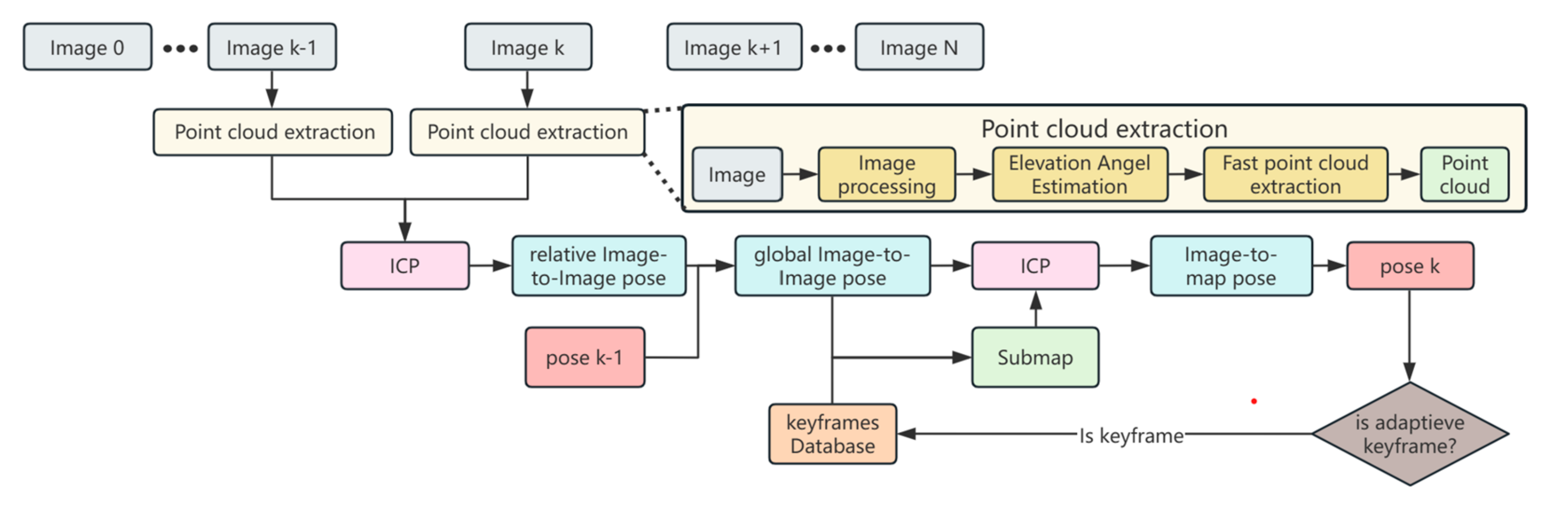
To overcome these limitations, this paper proposes DFLSO. Its algorithm framework is shown in the Figure 1, aiming to quickly and directly obtain the pose estimation result of the current FLS image. There are two core contributions: Firstly, a lightweight FLS image processing technique is developed, which can extract 3-D point clouds from FLS images. By using point cloud matching instead of image matching, the pose errors caused by the nonlinearity of the projection model are reduced. Secondly, a method for quickly constructing a local submap using past overlapping images is designed. By matching the point cloud of the current image with the submap, the cumulative errors based on odometry are reduced. This enhances the global pose consistency without relying on the accuracy of loop closure detection or waiting for a loop closure to be detected.
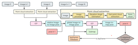
Figure 1.
The DFLSO framework.
3. Methods
3.1. FLS Projection Model
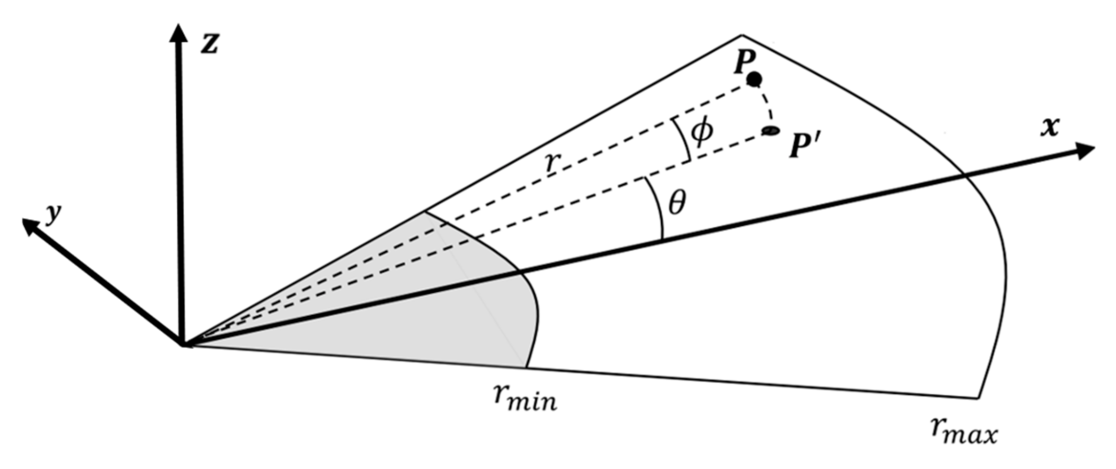
FLS can simultaneously transmit and receive multiple fan-shaped acoustic beams along different azimuth angle directions. Each beam has a narrow azimuth opening angle and a wide elevation opening angle, with the ranges covered by these acoustic beams collectively forming the field of view of FLS. As shown in Figure 2 and Equation (1), a 3-D point P in FLS coordinates can be described as (x, y, z) in Cartesian coordinates, and (r, θ, ϕ) in polar coordinates.

Figure 2.
Projection model of FLS.
Actually, FLS only generates 2-D images. The imaging plane of FLS images can be conceptualized as a horizontal plane formed by the X and Y axes within the FLS’s coordinate system. During the projection process, only the azimuth angle and distance of the echo are received, resulting in the loss of elevation angle and the elevation angle is assumed to be zero in this process. Thus, a 3-D point P is projected onto this 2-D imaging plane as P′, with the coordinates shown in Equation (2):
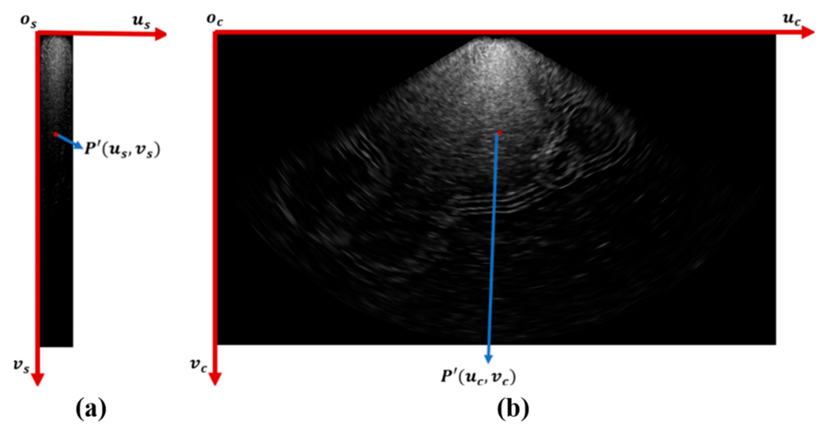
The point P′ ultimately needs to be presented on the pixel plane. FLS receives the echo intensity at different distance bins for each beam and generates a raw beam-bin image. Define the pixel coordinate system of the beam-bin image as os–us–vs, with the origin os located at the top-left corner, and the us-axis and vs-axis as shown in Figure 3a. Assume that the sonar configuration parameters include N acoustic beams, and each beam can measure the echo intensity at M bins, with the minimum and maximum detection distances being rmin and rmax, and the minimum and maximum detection azimuth angles being θmin and θmax. The point P′(us, vs) in the beam-bin image are given by Equation (3).

Figure 3.
Different forms of FLS images. (a) Beam-bin image in polar pixel plane. (b) Image in Cartesian pixel plane.
FLS images can also be interpolated into a Cartesian pixel plane. Define the pixel coordinate system as oc–uc–vc, with the origin oc at the top-left corner, the uc-axis and vc-axis as shown in Figure 3b. The coordinates of point P′(uc, vc) are given by Equation (4).
where umax denotes the width of the image, fu and fv are the scaling factors between the pixel space of the interpolated image and the physical space along the us and vs axes, respectively. These scaling factors are typically expressed in pixels per meter and are generally equal along both axes.
3.2. Point Cloud Extraction from Image
The grayscale value of each pixel in a FLS image is directly correlated with echo intensity, which is influenced by factors such as the acoustic beam’s propagation distance, reflection angle, and the acoustic properties of the reflecting surface. Typically, flat seabed terrain exhibits moderate echo intensity. In contrast, areas with rocks or protruding terrain display stronger echo intensity and accompanied by shadow regions with weaker intensity formed by the acoustic beam being blocked by the height of obstacles. Similarly, abrupt depressions, such as trenches or gullies, also produce shadow regions of weaker echo intensity. By segmenting the FLS image into three distinct regions: highlight, shadow, and background, it becomes possible to identify and extract seabed features associated with these regions. Specifically, highlight–shadow pairs generated by protruding terrain or rocks, as well as shadow features resulting from depressions, can be analyzed. Through the examination of their spatial positions and shadow lengths within the image, these terrain features can be extracted and represented as 3-D point clouds.
3.2.1. Image Processing
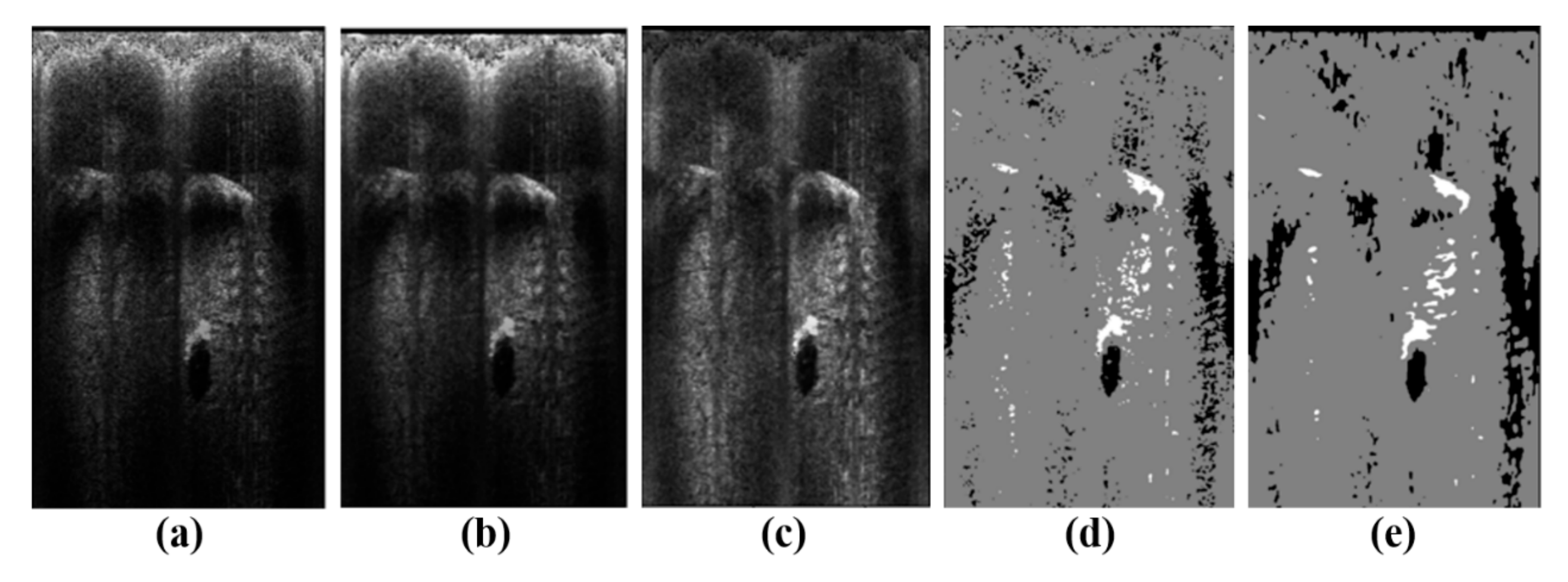
The objective of image processing is to classify each pixel in the FLS image based on its grayscale value into highlight, shadow, and background regions. This classification facilitates the extraction of highlight and shadow features, which are essential for subsequent calculations of the height and position of terrain features to form a 3-D point cloud. Firstly, FLS images are often contaminated with salt-pepper noise, which can be mitigated using a median filter, as shown in Figure 4b. Secondly, as acoustic beams propagate further, their intensity attenuates, leading to lower grayscale values in pixels corresponding to farther regions. The gain compensation coefficients for each distance are computed by averaging the grayscale values of pixels at the same distance along different azimuth angles in the image, thus compensating for the grayscale value differences caused by propagation distance, as shown in Figure 4c. Thirdly, the compensated pixels are classified based on their grayscale values. Given that only three categories are required, the k-means clustering method is chosen to perform the image segmentation, as shown in Figure 4d. Finally, the fast extraction method for 3-D point clouds in this work demands the preservation of the completeness of the highlight and shadow region features in the image. Consequently, morphological processing is applied to the segmented image. Specifically, an erosion operation is first employed to remove small highlight and shadow regions resembling noise, followed by a dilation operation to complete the damaged highlight and shadow regions, as shown in Figure 4e.

Figure 4.
Preprocessing of FLS images. (a) Raw beam-bin image. (b) Image after median filter. (c) Image after gain compensation. (d) Image after segmentation. (e) Image after morphological processing.
3.2.2. Elevation Angle Estimation
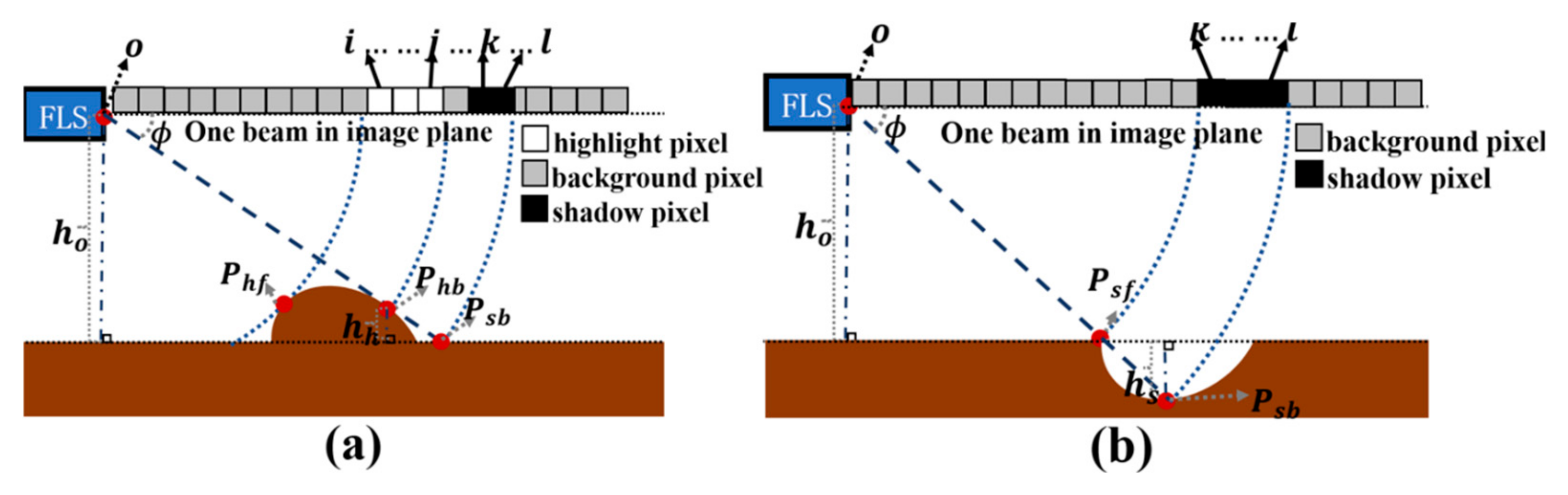
In FLS images, if some highlight pixels are immediately followed by shadow pixels, these pixels correspond to an acoustic beam encountering a protruding terrain with a certain height on the seabed. The shadow region is formed due to the elevation difference between the protruding terrain and the seabed, which blocks the sound waves. The length of shadow region can be used to calculate the elevation and elevation angle of the protruding terrain. Assuming the seabed around the protruding terrain is flat, the geometric relationship of elevation and shadow length in one acoustic beam is shown in Figure 5a. O represents the point where the FLS transmits and receives acoustic beams. Phb is the point where the protruding terrain begins to block the acoustic beam, and Psb is the point where the protruding terrain no longer blocks the acoustic beam. With the ideal model, Phb and Psb share the same elevation angle ϕ. Therefore, the elevation hh and elevation angle can be calculated using the elevation ho of the FLS above the seabed and the distances from point O to Phb and Psb by Equation (5).

Figure 5.
Geometric relationship between shadow length and seabed terrain. (a) Protruding terrain. (b) Depression terrain.
The elevation of FLS ho is a fixed value for some underwater robots operating close to the seabed, such as deep-sea mining vehicles or trenchers. For robots that float in the water, this elevation ho can be measured using an altimeter. The distances of |OPhb| and |OPsb| can be calculated by identifying the pixel positions corresponding to Phb and Psb in the image column. Point Phb corresponds to the transition boundary from the highlight region to the shadow region. However, in actual FLS images, the transition does not occur directly from the highlight region to the shadow region but includes a small transition background area. Therefore, the end pixel of the highlight region is defined as the corresponding pixel for point Phb, denoted as the j-th pixel. Point Psb corresponds to the position where the protruding terrain no longer blocks the acoustic beam, which is the transition point from the shadow region to the background region. Here, the end pixel of the shadow region is defined as the corresponding pixel for point Psb, denoted as the l-th pixel. The distances |OPhb| and |OPsb| can be calculated with j and l based on Equation (4).
The depression terrain on the seabed will form a shadow region without a corresponding highlight region. The geometric model based on the planar assumption is shown in Figure 5b. In this case, the points Psf and Psb should theoretically have the same elevation angel ϕ. The elevation between point Psb and the seabed plane can be calculated based on the geometric relationships by Equation (6). It should be noted that the elevation hs is negative here.
The distances of |OPsf| and |OPsb| can be determined by identifying the pixel positions corresponding to points Psf and Psb in the image column. Point Psf corresponds to the transition boundary from the background region to the shadow region, which is set as the front pixel of the shadow region, denoted as the k-th pixel. Point Psb corresponds to the transition boundary from the shadow region to the background region, which is defined as the end pixel of the shadow region, denoted as the l-th pixel. The distances |OPsf| and |OPsb| can also be calculated with k and l based on Equation (4).
3.2.3. Fast Point Cloud Extraction
In Section 3.2.2, the elevation and elevation angle of the end pixels of highlight or shadow regions in the FLS image can be calculated, thereby obtaining the 3-D coordinates of the corresponding points. However, the number of edge points obtained through this method is limited. When employing point cloud matching, it is advantageous to have a greater number of 3-D points to form a comprehensive point cloud. Several researchers have developed reconstruction methods to recover 3-D information about object surfaces, such as utilizing the elevation of the end pixel of the highlight region and constructing relationships between grayscale, reflection angle, and elevation for each highlight pixel to iteratively solve for the 3-D shape of the object’s surface [28]. However, these reconstruction methods often oversimplify the propagation and reflection models of acoustic beams, which may lead to inaccuracies in the results. Additionally, they require multiple iterative solutions, imposing a significant computational burden that makes real-time computation challenging.
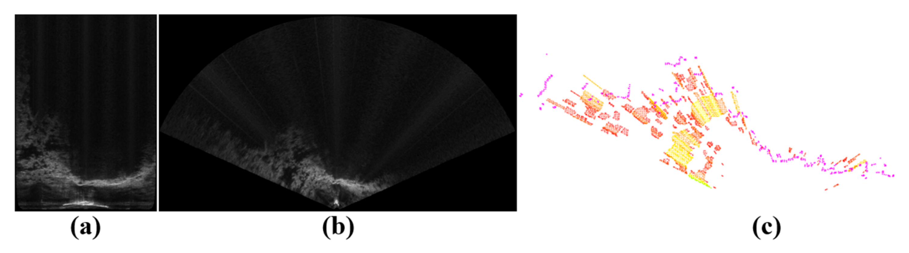
This paper aims to implement a fast method for obtaining an approximate point cloud of the seabed. To achieve this, the elevation at the end pixel is assumed to be representative of the entire region. Specifically, for highlight–shadow regions of protruding terrain, the elevation of the end highlight pixel is used to represent the elevation of each pixel within the highlight region, and the elevation angle is then calculated to determine its 3-D coordinates. For isolated shadow regions of depressed terrain, the elevation corresponding to the end shadow pixel in the column is used to represent the elevations of all pixels within the shadow region, and the elevation angle and 3-D coordinates are subsequently calculated. While this approach may introduce some discrepancies in elevation and horizontal size between the point cloud and the actual protruding or depressed terrain, it enables the rapid acquisition of an approximate point cloud of the seabed. Figure 6 shows an example of extracting point cloud from an FLS image.
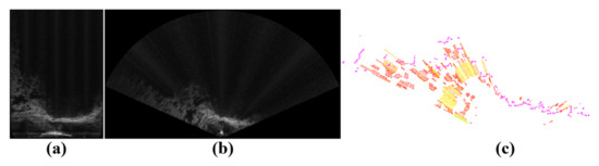
Figure 6.
An example of extracting point cloud from an FLS image. (a) Beam-bin image. (b) Image in Cartesian pixel plane. (c) The 3-D point cloud from this image.
3.3. Image-to-Image
In the first stage of DFLSO, it is necessary to match FLS images sampled at adjacent time instants to obtain the relative transformation of the robot’s pose at the time of image acquisition. Pk is defined as the point cloud extracted from the FLS image at time tk. And Xk, k−1 (Xk, k−1 ∈ SE (3)) is defined as the relative transformation between the robot’s pose at time tk−1 and time tk. Therefore, the problem is transformed into a classical point cloud registration problem as shown in Equation (7), which involves finding a relative transformation Xk, k−1 to make the distance between corresponding points in Pk and Pk−1 is minimized.
This paper uses the classical Iterative Closest Point (ICP) algorithm [29] for point cloud registration. The ICP algorithm is a classic method for 3-D point cloud matching, aiming to find the optimal rigid transformation between two point clouds. First, transform the source point cloud Pk using the transformation Xk, k−1, and for each point in the source point cloud Pk, the algorithm finds the closest point in the target point cloud Pk−1 as its corresponding point. Second, based on the corresponding point-pairs found in the previous step, the algorithm calculates the rigid transformation Xk, k−1 that minimizes the sum of squared distances between the corresponding points. Repeat the above steps until a convergence condition is met, such as the increment of the transformation being smaller than a certain threshold. The ICP algorithm needs an initial value for the transformation Xk, k−1. If prior information about the relative pose transformation can be obtained from an IMU or other sensors, we use this prior as the initial value for the registration. Otherwise, we assume that the robot’s attitude and position changes are small, and use an initial value of Xk, k−1 = I for the registration.
3.4. Submap and Image-to-Map Match
In the first stage, the relative transformation between adjacent FLS images obtained through image-to image matching is combined with the previous global pose to generate an initial estimate of the current pose. To enhance global consistency and mitigate potential cumulative errors, a second stage of image to-map matching is employed. Here, the global pose at time tk is denoted as XWk and the point cloud of submap is denoted as PWm. This image-to-map matching is formulated as a classical point cloud registration problem, as shown in Equation (8).
A key innovation in this work lies in the generation of a point cloud of submap for image-to-map matching. Instead of directly accumulating all historical point clouds, this work keeps a history of keyframes, where each keyframe consists of an image paired with its corresponding global pose. For the image-to-map matching, the submap point cloud is generated by searching for a subset of keyframes that have a co-visibility relationship with the current image.
3.4.1. Keyframe Selection for Submap
In this study, we propose principles for selecting appropriate keyframes to construct a submap for matching, focusing on minimizing odometry cumulative error and enhancing global pose consistency. To address cumulative errors, we employ a K-Nearest Neighbors (KNN) search to identify keyframes closest to the current pose, ensuring overlapping terrain features with the current image. By including them in the submap, the cumulative error between the current pose and the selected nearby poses is minimized.
Additionally, to improve global consistency, we incorporate earlier keyframes whose fields of view (FoV) overlap with the current sonar image’s FoV, including these older keyframes in the submap helps enhance the global consistency of the pose derived from image-to-map matching. Notably, FLS observes only a front-facing sector of the environment, unlike LiDAR which provides 360° coverage. This work defines the FoV center as the point located at half of the maximum observation distance in the FLS coordinate system directly, as shown in Figure 7. Consequently, the center of the FoV for each keyframe can be computed based on the global pose of the keyframe. Using the FoV centers, we perform a KNN search to select keyframes that enhance global pose consistency, crucial for underwater robots performing round-trip inspections, thereby improving localization accuracy and robustness.
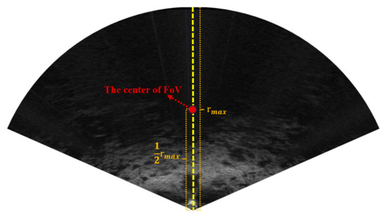
Figure 7.
The center of FLS’s field of view.
3.4.2. Adaptive Keyframing
The selection of images and their corresponding poses for keyframe designation significantly impacts the construction of the submap and the accuracy and robustness of the image-to-map matching process. Traditional approaches typically employ fixed thresholds for keyframe addition, where a keyframe is inserted when changes in position or orientation exceed predefined values. The keyframe should ideally aim to cover the entire environmental space with a minimal number. To address this, adaptive thresholds for keyframe insertion were proposed in [30], where the thresholds are dynamically adjusted based on spatial information derived from the image. Specifically, when the point clouds are distributed at greater distances, features at large distances remain visible even after significant displacement, making them suitable for matching. In such cases, the distance threshold can be larger. Conversely, if the point clouds are concentrated close to the FLS, even minor positional changes can cause nearby features to disappear from the image, rendering them unsuitable for matching. Thus, a smaller distance threshold is required in such scenarios. The distance threshold dthk for current image at time tk can vary adaptively by the median Euclidean point distance mk from the FLS to each point in the point cloud extracted from current image by Equation (9).
The rotational threshold is derived from the horizontal opening angle of FLS, and is set to 1/6 of this angle in this work. After the current image undergoes two-stage matching to obtain its global pose, the distance and rotational thresholds are computed based on the point cloud. If the positional or orientational changes between the current pose and the pose of the previous keyframe exceed these thresholds, the current image and its global pose are added to the set of keyframes.
3.4.3. Fast Keyframe-Based Submapping
For the seabed point clouds extracted from FLS images, the accuracy of the elevation information depends on the precision of the shadow region segmentation, which cannot achieve the same accuracy as the lidar. As a result, points associated with the same horizontal region across different images may exhibit variations in elevation. Simply stacking the point clouds from multiple keyframes can introduce “ghosting” artifacts in the representation of the seabed surface, thereby compromising the reliability of the image-to-map matching process.
To mitigate this issue, in this work, we perform a grid-based rasterization of the seabed space on the horizontal plane. Specifically, we create a grid map on the horizontal expanse of the seabed area. Each cell in this grid map serves as a discrete unit for processing. For every grid cell in the grid map, we aggregate the points contained within it into a single representative point. The elevation and horizontal position of this representative point are computed as the average of all the points from each keyframe that fall within that specific grid cell. This averaging mechanism effectively reduces the impact of elevation inconsistencies of different keyframes.
Once the submap point cloud is constructed from the selected keyframes, the ICP method is employed to match the current image’s point cloud with the submap, thereby facilitating accurate image-to-map matching and enabling the determination of the global pose.
4. Experiment and Discussion
4.1. Simulation Experiment
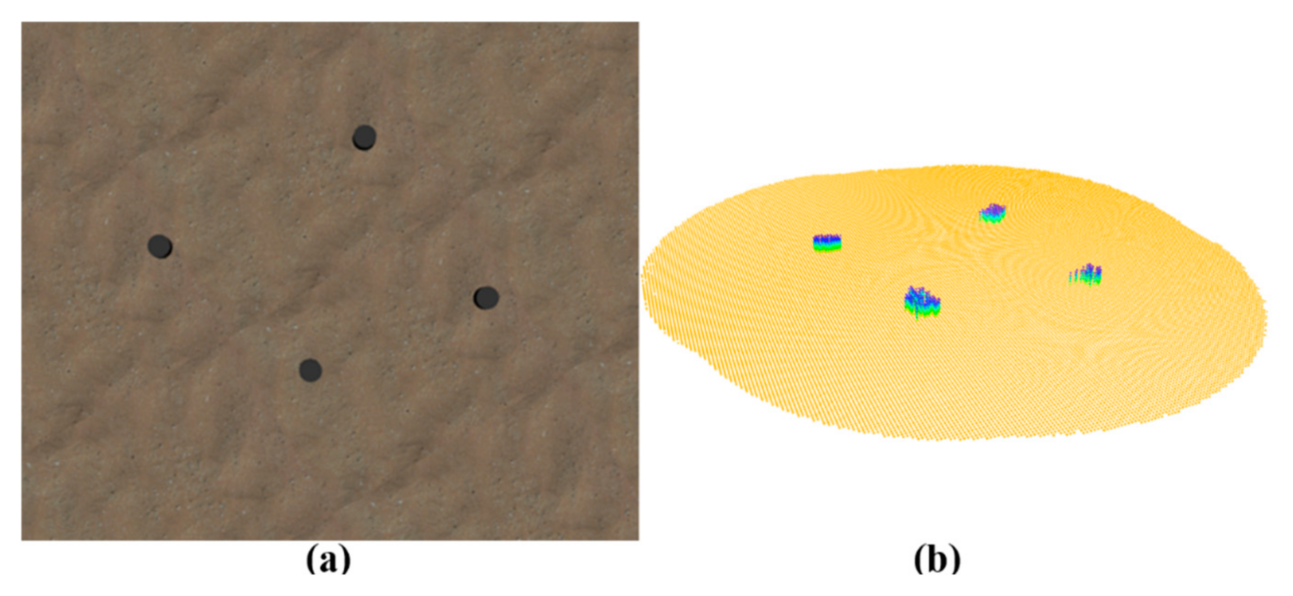
In underwater experiments, obtaining the true pose of an underwater robot is challenging. Therefore, the proposed DFLSO was validated through a simulation experiment. The simulations were conducted using ROS (Robot Operating System) in the Gazebo physics simulation environment, with the FLS simulated using the open-source UUV-Simulator [31]. In the simulation, the FLS was maintained at a fixed elevation of 2 m above the seabed, the azimuth opening angle is set as 45°, the elevation opening angle is set 30°, the detection range is set as 8 m and the imaging frame rate is set as 10 hz. The simulation environment was set on a sandy seabed and included several rocks as terrain features, as shown in Figure 8a. Figure 8b displays the seabed point cloud map constructed using all the keyframes. To provide a more intuitive visualization of the point cloud heights, after filtering the points within the horizontal grids, the points were filled from the seabed plane to their respective heights.
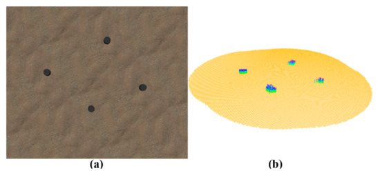
Figure 8.
Simulation environment and mapping results. (a) Simulation environment in Gazebo. (b) Seabed point cloud map.
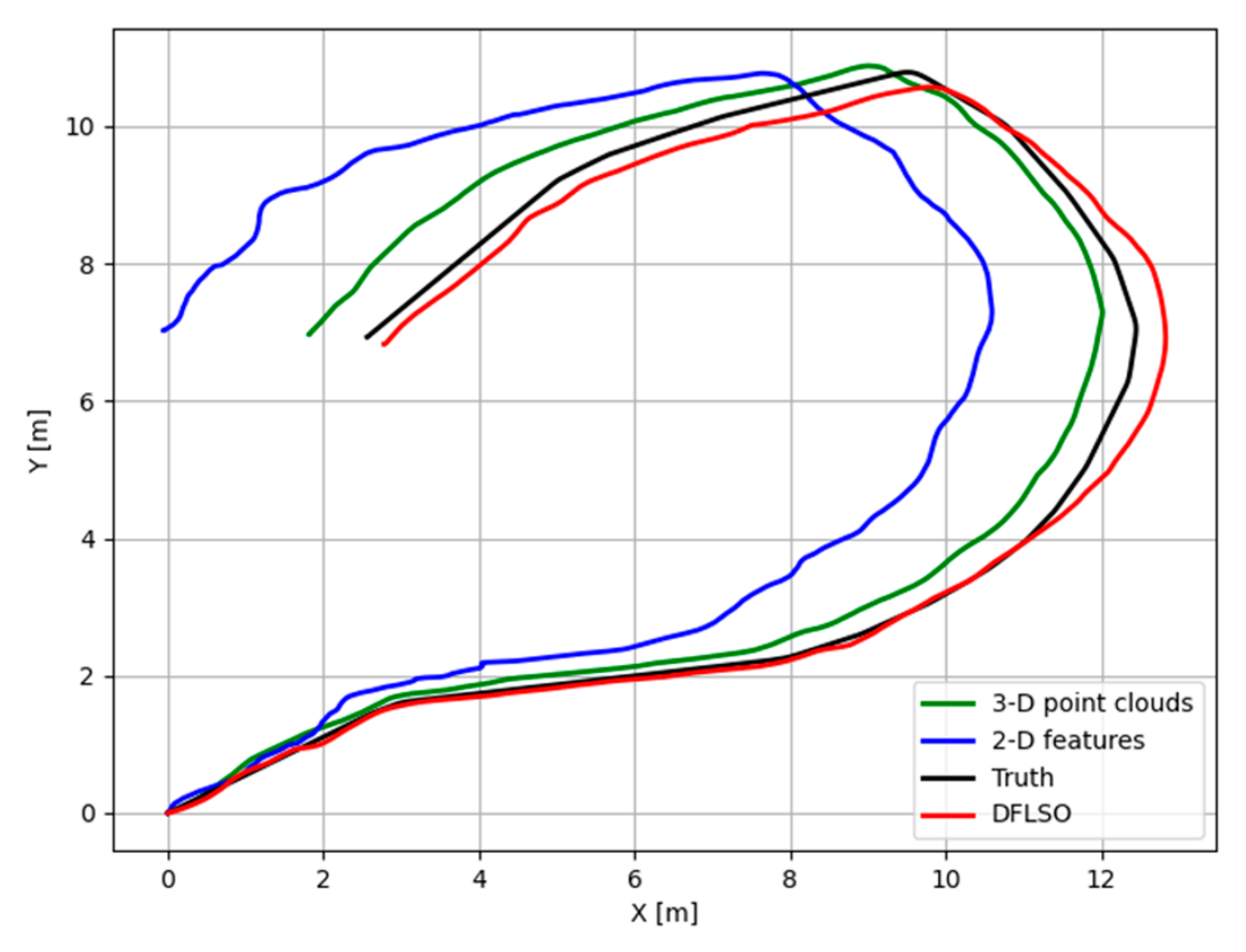
In the simulation experiment, three different odometry methods are compared: the first method (2-D features) [12] extracts 2-D features with large gradient changes in the FLS images and performing image-to-image matching for odometry estimation. The second method (3-D point clouds) [15] estimates the elevation through shaded area to form 3-D feature point clouds and use ICP-based algorithm for matching. The third method is the proposed DFLSO approach, which incorporated both image-to-image and image-to-map matching using the extracted 3-D point clouds; the number of keyframes for each submap is set as 6. The data was processed using a 16-core Intel Ultra 9 2.90 GHz CPU. In this simulation, the average processing times per image for the 2-D features, 3-D point clouds, and DFLSO are 14.6 ms, 24.8 ms, and 32.7 ms, respectively. Although both extracting 3-D point clouds and constructing submaps for two-stage matching will lead to an increase in computing time, with the fast point cloud extraction and submap construction methods proposed in this paper, the increased computing time can still meet the real-time requirements.
The trajectories for different methods are shown in Figure 9. Here, use the absolute position errors (APE) to evaluate the accuracy, which are shown in Figure 10, and some statistical metrics are summarized in Table 1. The APE used in this paper focuses on the deviation in the horizontal direction between the estimated position and its true position, as shown in Equation (10). Where and are the estimated position in the x-direction and y-direction, and are the ground-truth.
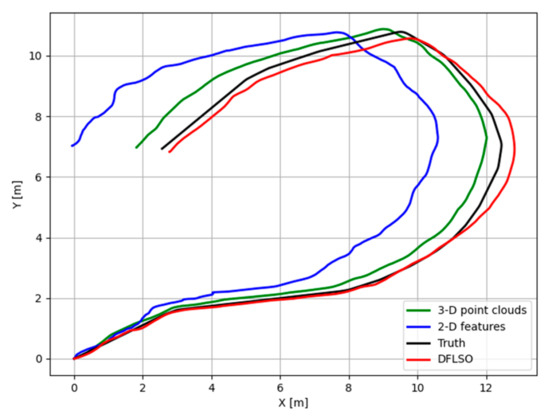
Figure 9.
Trajectories for different methods in the simulation.
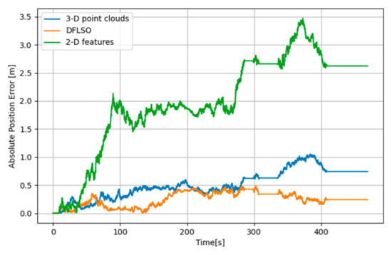
Figure 10.
Error comparison for different methods in the simulation.

Table 1.
Evaluation of different odometry methods in the simulation.
Compared to the 2-D feature-based approach, using the 3-D point clouds extracted from the FLS images achieves more accurate localization results. Furthermore, a comparison between the 3-D point cloud based matching method and the DFLSO approach revealed that the proposed image-to-map matching stage effectively mitigated the accumulation of errors and significantly improved the global consistency of the localization results.
4.2. Field Experiment
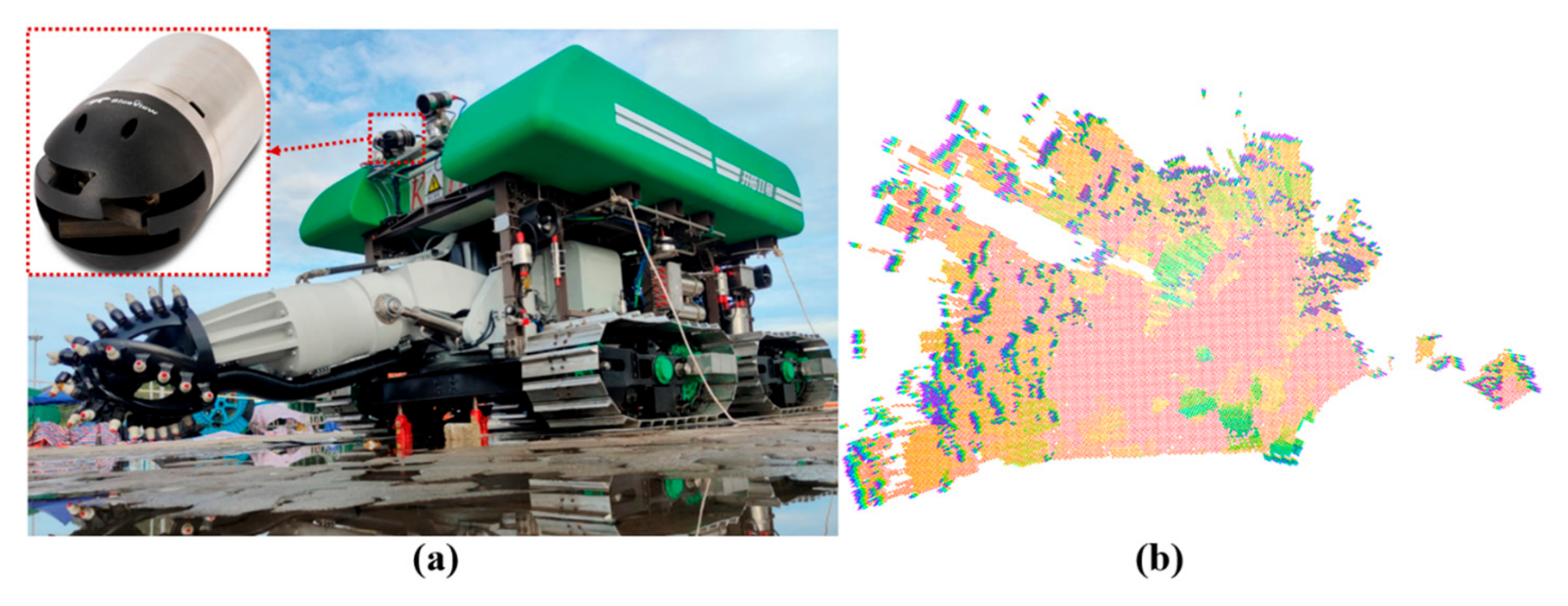
The proposed DFLSO was also tested with field data, and the number of keyframes for each submap was set as 6. We constructed a tracked deep-sea underwater robot, which is a cable robot equipped with a BlueView M900 FLS shown in Figure 11a. The robot was tested at a depth of 2000 m in July 2024. During this sea trial, the FLS is set to have an azimuth opening angle of 120°, an elevation opening angle of 20°, a detection range of 50 m, and an imaging frequency of 15 Hz. The FLS communicates via Ethernet, and the data is transmitted in real-time to the computer on board through the optical fiber in the cable. Data processing and recording are then carried out on the computer on board.

Figure 11.
The tracked underwater robot with FLS and the mapping result of the sea trial. (a) the tracked deep-sea underwater robot (b) the mapping result of the sea trial.
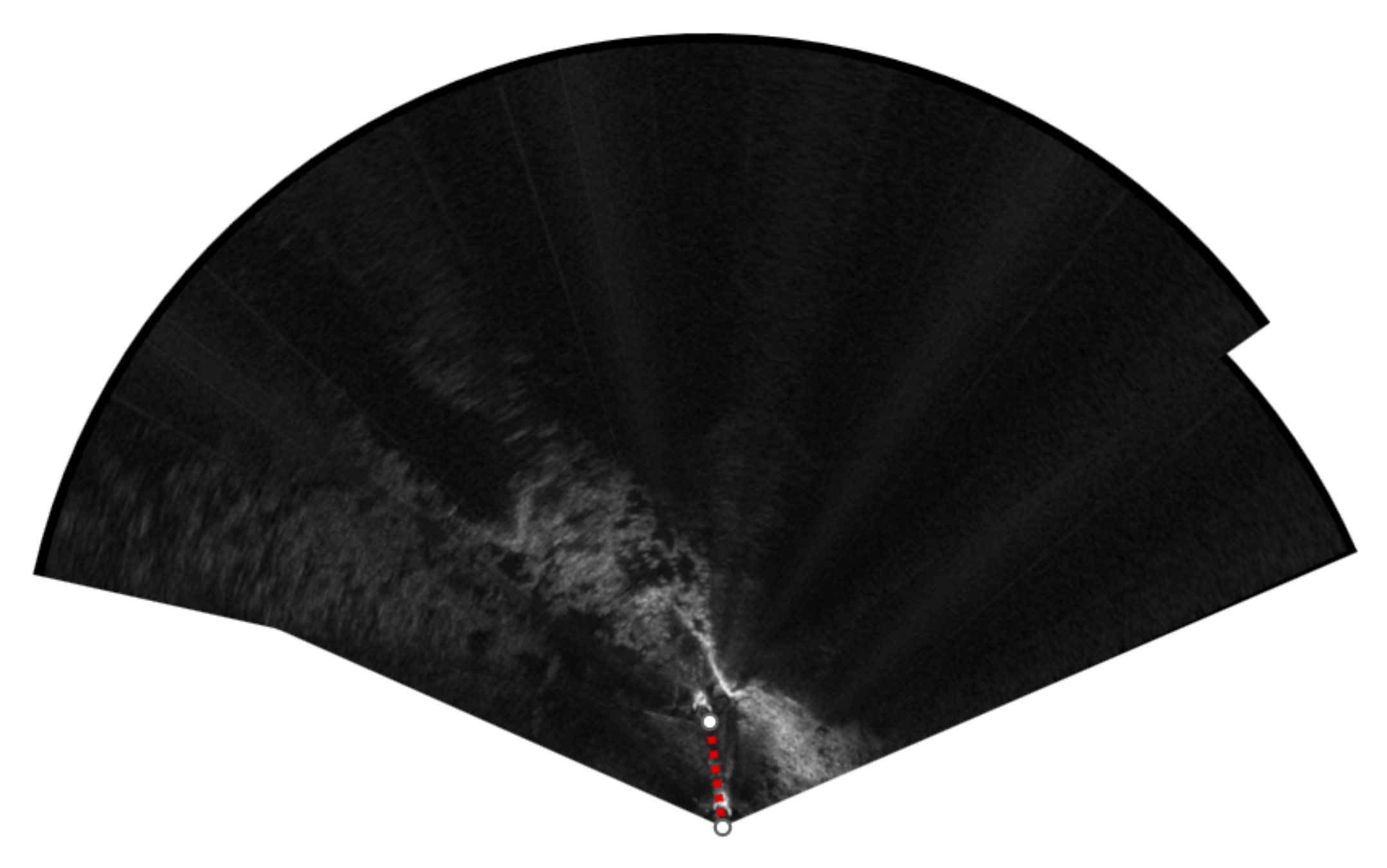
The sea trial has a rugged seabed with many topographical features, and the mapping result with DFLSO is shown in Figure 11b. During the sea trials, it was challenging to obtain the true position of the underwater robot. Therefore, to determine the true position of the selected reference points, we manually registered the FLS images sampled at different reference points, as shown in Figure 12. This process allowed us to establish the truth to evaluate the odometry results. The data was processed using a 16-core Intel Ultra 9 2.90 GHz CPU. With the FLS images in this field experiment, the average processing times per image for the 2-D features, 3-D point clouds, and DFLSO are 27.4 ms, 38.5 ms, and 52.6 ms, respectively.

Figure 12.
Example of manual registering of FLS images.
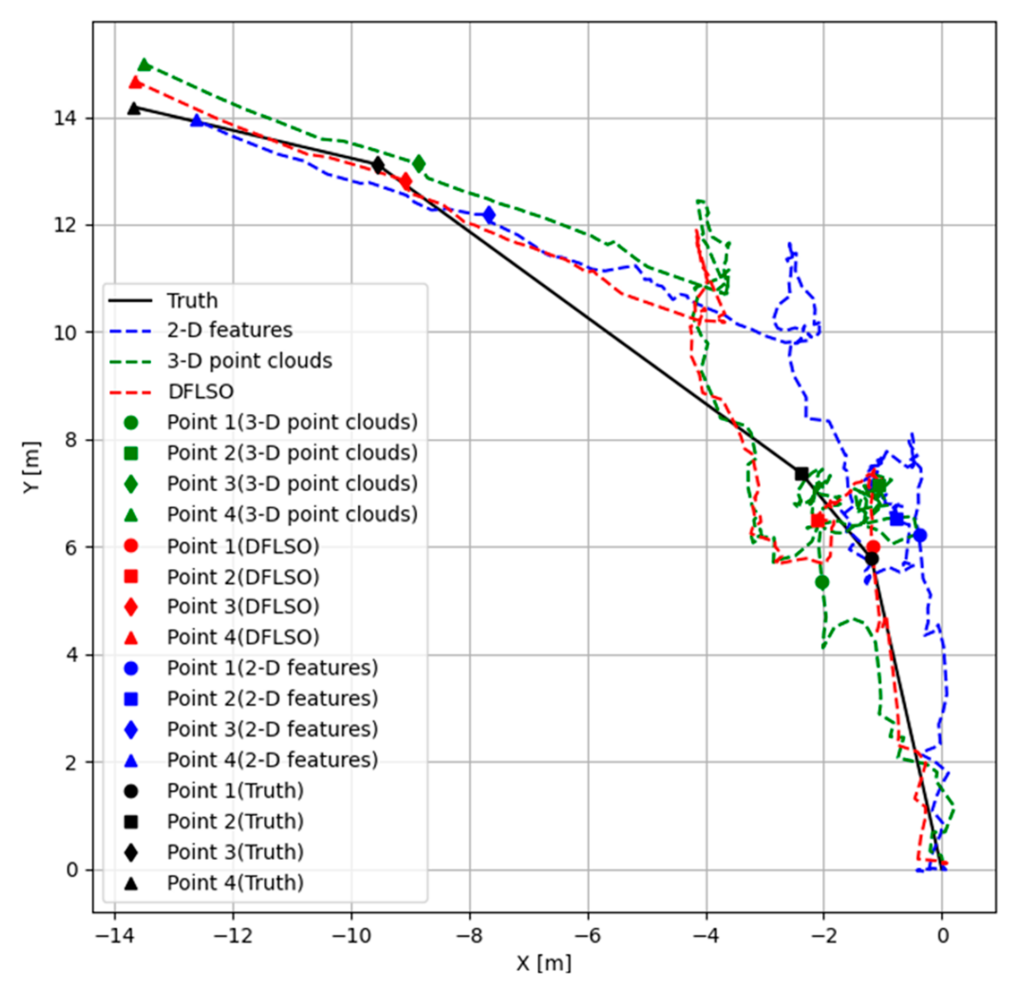
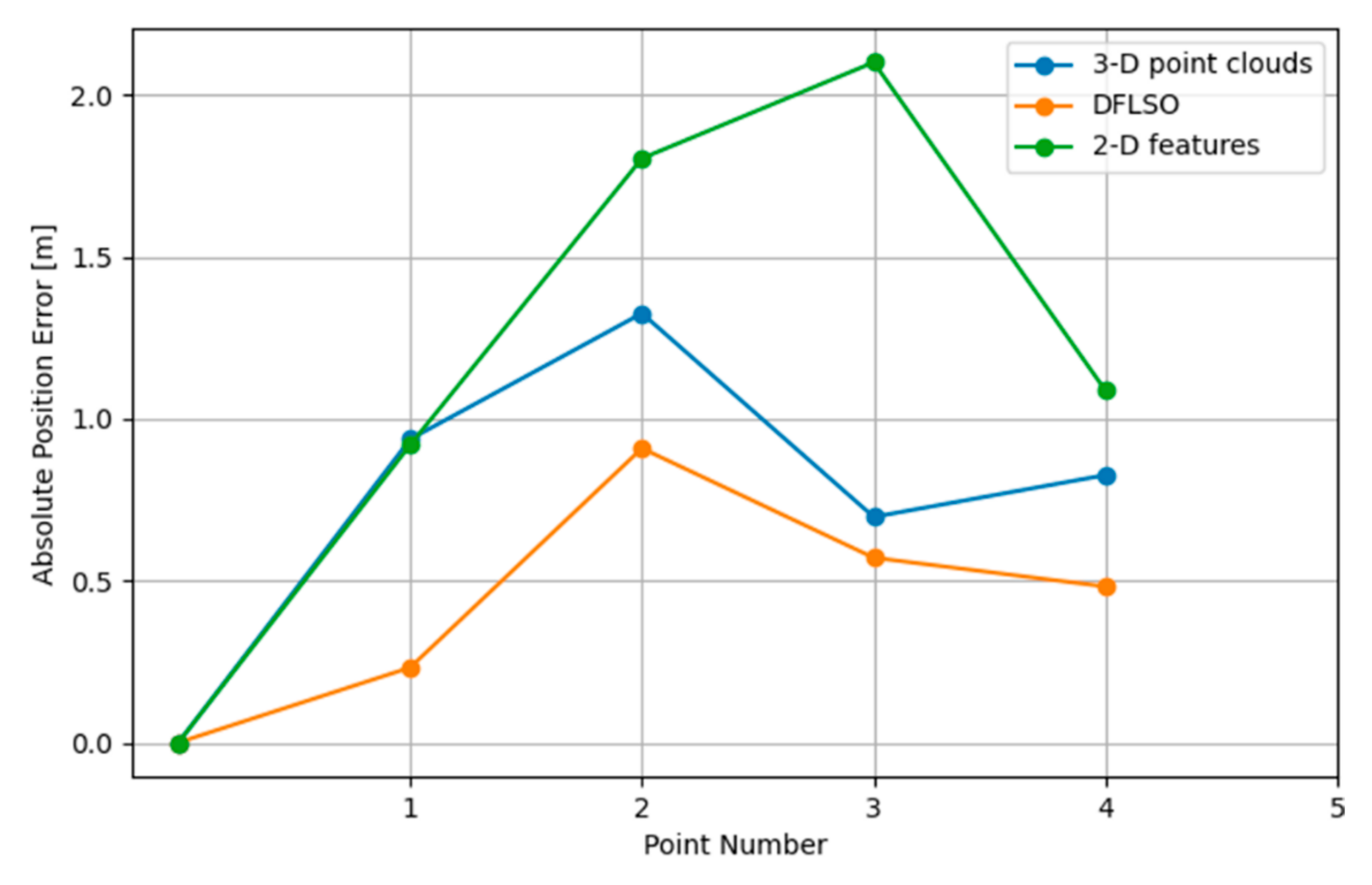
Four reference points were selected to quantitatively evaluate the positioning results, and the trajectories of the three methods are shown in Figure 13, the APE of each method relative to the reference points are shown in Figure 14, and statistical metrics are summarized in Table 2. The truth was obtained by directly connecting the reference points with straight lines, which represents the true trend of movement but does not necessarily imply that the robot traveled in a straight line between reference points. Notably, the DFLSO method proposed in this paper achieves the closest approximation to the true values of the reference point positions. These findings demonstrate the feasibility and superiority of the DFLSO method in a real seabed. By comparing the results of the method based on 2-D features and 3-D point clouds, it can be seen that using the 3-D point clouds extracted from the images for matching can improve the accuracy of the relative pose. By comparing the odometry results of the method based on 3-D point clouds and DFLSO, it can also be seen that the matching between the images and the submap effectively improves the positioning accuracy.
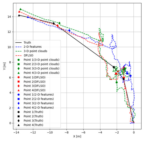
Figure 13.
Trajectories for different methods in the sea trial.

Figure 14.
APE for different methods in the sea trial.
Table 2.
Evaluation of different odometry methods in the field experiment.
5. Conclusions
This work presents the DFLSO, a lightweight front-end FLS odometry for underwater robot localization. The key innovation lies in proposing a lightweight image processing method that rapidly extracts approximate point clouds of the seabed terrain, enabling point cloud matching for odometry estimation, avoiding pose errors caused by image ambiguities when directly using image matching for localization. Secondly, the work develops a fast keyframe-based point cloud submapping method for FLS images. The point cloud of submap can realize image-to-map matching for FLS images, which can improve the pose global consistency and mitigate the accumulation of odometry errors. The reliability of the proposed DFLSO is validated through both simulation experiments and field trials, demonstrating its capability to provide high-precision localization for underwater robots in real-world scenarios, which would contribute to higher-precision localization, operation, and observation capabilities, reducing the omission or repetition of operation areas.
Author Contributions
Conceptualization, W.X.; methodology, W.X.; software, W.X. and X.L.; validation, W.X., J.M. and H.L.; formal analysis, W.X.; investigation, J.Y.; resources, W.X.; data curation, W.X.; writing—original draft preparation, W.X.; writing—review and editing, J.Y.; visualization, C.L. and X.L.; supervision, J.Y.; project administration, J.Y.; funding acquisition, J.Y. All authors have read and agreed to the published version of the manuscript.
Funding
This research was funded by the Science and Technology Committee Shanghai Municipality (19DZ1207300) and the Major Projects of Strategic Emerging Industries in Shanghai (BH3230001).
Data Availability Statement
The data presented in this study are available on request from the corresponding author.
Acknowledgments
The authors would like to thank the anonymous reviewers for their constructive suggestions which comprehensively improve the quality of the paper.
Conflicts of Interest
The authors declare no conflicts of interest.
References
- Martin, E.J.; Caress, D.W.; Thomas, H.; Hobson, B.; Henthorn, R.; Risi, M.; Paull, C.K.; Barry, J.P.; Troni, G. Enabling New Techniques in Environmental Assessment Through Multi-Sensor Hydrography. In Proceedings of the Oceans 2016 Mts/IEEE Monterey, Monterey, CA, USA, 19–23 September 2016. [Google Scholar] [CrossRef]
- Leng, D.X.; Shao, S.; Xie, Y.C.; Wang, H.H.; Liu, G.J. A brief review of recent progress on deep sea mining vehicle. Ocean. Eng. 2021, 228, 108568. [Google Scholar] [CrossRef]
- Hasan, K.; Ahmad, S.; Liaf, A.F.; Karimi, M.; Ahmed, T.; Shawon, M.A.; Mekhilef, S. Oceanic Challenges to Technological Solutions: A Review of Autonomous Underwater Vehicle Path Technologies in Biomimicry, Control, Navigation, and Sensing. IEEE Access 2024, 12, 46202–46231. [Google Scholar] [CrossRef]
- Paull, L.; Saeedi, S.; Seto, M.; Li, H. AUV Navigation and Localization: A Review. IEEE J. Ocean. Eng. 2014, 39, 131–149. [Google Scholar] [CrossRef]
- Hidalgo, F.; Braunl, T. Review of Underwater SLAM Techniques. In Proceedings of the 2015 6th International Conference on Automation, Robotics and Applications (Icara), Queenstown, The Netherlands, 17–19 February 2015; pp. 306–311. [Google Scholar]
- González-García, J.; Gómez-Espinosa, A.; Cuan-Urquizo, E.; García-Valdovinos, L.G.; Salgado-Jiménez, T.; Cabello, J.A.E. Autonomous Underwater Vehicles: Localization, Navigation, and Communication for Collaborative Missions. Appl. Sci. 2020, 10, 1256. [Google Scholar] [CrossRef]
- Westman, E.; Kaess, M. Degeneracy-Aware Imaging Sonar Simultaneous Localization and Mapping. IEEE J. Ocean. Eng. 2020, 45, 1280–1294. [Google Scholar] [CrossRef]
- Wang, Y.S.; Ji, Y.; Woo, H.; Tamura, Y.; Tsuchiya, H.; Yamashita, A.; Asama, H. Acoustic Camera-Based Pose Graph SLAM for Dense 3-D Mapping in Underwater Environments. IEEE J. Ocean. Eng. 2021, 46, 829–847. [Google Scholar] [CrossRef]
- Sekkati, H.; Negahdaripour, S. 3-D Motion Estimation for Positioning from 2-D Acoustic Video Imagery; Lecture Notes in Computer; Science; Springer: Berlin/Heidelberg, Germany, 2007; Volume 4478, pp. 80–88. [Google Scholar]
- Wang, Y.S.; Ji, Y.; Tsuchiya, H.; Ota, J.; Asama, H.; Yamashita, A. Acoustic-N-Point for Solving 2D Forward Looking Sonar Pose Estimation. IEEE Robot. Autom. Let. 2024, 9, 1652–1659. [Google Scholar] [CrossRef]
- Hurtos, N.; Nagappa, S.; Cufi, X.; Petillot, Y.; Salvi, J. Evaluation of Registration Methods on Two-Dimensional Forward-Looking Sonar Imagery. In Proceedings of the 2013 Mts/Ieee Oceans-Bergen, Bergen, Norway, 10–14 June 2013. [Google Scholar]
- Johannsson, H.; Kaess, M.; Englot, B.; Hover, F.; Leonard, J. Imaging Sonar-Aided Navigation for Autonomous Underwater Harbor Surveillance. In Proceedings of the IEEE/RSJ 2010 International Conference on Intelligent Robots and Systems (Iros 2010), Taipei, Taiwan, 18–22 October 2010; pp. 4396–4403. [Google Scholar] [CrossRef]
- Aykin, M.D.; Negahdaripour, S. On Feature Extraction and Region Matching for Forward Scan Sonar Imaging. In Proceedings of the 2012 Oceans, Hampton Roads, VA, USA, 14–19 October 2012. [Google Scholar]
- Negahdaripour, S. On 3-D Motion Estimation From Feature Tracks in 2-D FS Sonar Video. IEEE Trans. Robot. 2013, 29, 1016–1030. [Google Scholar] [CrossRef]
- Lee, G.; Yoon, S.; Lee, Y.; Lee, J. Improving ICP-Based Scanning Sonar Image Matching Performance Through Height Estimation of Feature Point Using Shaded Area. J. Mar. Sci. Eng. 2025, 13, 150. [Google Scholar] [CrossRef]
- Hurtos, N.; Ribas, D.; Cufi, X.; Petillot, Y.; Salvi, J. Fourier-based Registration for Robust Forward-looking Sonar Mosaicing in Low-visibility Underwater Environments. J. Field Robot. 2015, 32, 123–151. [Google Scholar] [CrossRef]
- Franchi, M.; Ridolfi, A.; Pagliai, M. A forward-looking SONAR and dynamic model-based AUV navigation strategy: Preliminary validation with FeelHippo AUV. Ocean Eng. 2020, 196, 106770. [Google Scholar] [CrossRef]
- Yoon, E.; Kim, B.; Joe, H. A Study on Acoustic Odometry Estimation based on the Image Similarity using Forward-looking Sonar. J. Sens. Sci. Technol. 2023, 32, 313–319. [Google Scholar] [CrossRef]
- Spears, A.; Howard, A.M.; West, M.; Collins, T. Determining Underwater Vehicle Movement from Sonar Data in Relatively Featureless Seafloor Tracking Missions. In Proceedings of the IEEE Winter Conference on Applications of Computer Vision, Steamboat Springs, CO, USA, 24–26 March 2014; pp. 909–916. [Google Scholar]
- Henson, B.T.; Zakharov, Y.V. Attitude-Trajectory Estimation for Forward-Looking Multibeam Sonar Based on Acoustic Image Registration. IEEE J. Ocean. Eng. 2019, 44, 753–766. [Google Scholar] [CrossRef]
- Almanza-Medina, J.E.; Henson, B.; Zakharov, Y.V. Deep Learning Architectures for Navigation Using Forward Looking Sonar Images. IEEE Access 2021, 9, 33880–33896. [Google Scholar] [CrossRef]
- Almanza-Medina, J.E.; Henson, B.; Zakharov, Y.V. Sonar FoV Segmentation for Motion Estimation Using DL Networks. IEEE Access 2022, 10, 25591–25604. [Google Scholar] [CrossRef]
- Muñoz, B.; Troni, G. Learning the Ego-Motion of an Underwater Imaging Sonar: A Comparative Experimental Evaluation of Novel CNN and RCNN Approaches. IEEE Robot. Autom. Let. 2024, 9, 2072–2079. [Google Scholar] [CrossRef]
- Fallon, M.F.; Folkesson, J.; McClelland, H.; Leonard, J.J. Relocating Underwater Features Autonomously Using Sonar-Based SLAM. IEEE J. Ocean. Eng. 2013, 38, 500–513. [Google Scholar] [CrossRef]
- Suresh, S.; Sodhi, P.; Mangelson, J.G.; Wettergreen, D.; Kaess, M. Active SLAM using 3D Submap Saliency for Underwater Volumetric Exploration. In Proceedings of the 2020 IEEE International Conference on Robotics and Automation (ICRA), Paris, France, 31 May 2020–31 August 2020. [Google Scholar]
- Li, J.; Kaess, M.; Eustice, R.M.; Johnson-Roberson, M. Pose-Graph SLAM Using Forward-Looking Sonar. IEEE Robot. Autom. Let. 2018, 3, 2330–2337. [Google Scholar] [CrossRef]
- Gaspar, A.R.; Matos, A. Feature-based place recognition using forward-looking sonar. J. Mar. Sci. Eng. 2023, 11, 2198. [Google Scholar] [CrossRef]
- Aykin, M.D.; Negahdaripour, S. Forward-Look 2-D Sonar Image Formation and 3-D Reconstruction. In Proceedings of the 2013 Oceans—San Diego, San Diego, CA, USA, 23–27 September 2013. [Google Scholar]
- Chen, Y.; Medioni, G. Object Modeling by Registration of Multiple Range Images. Image Vision. Comput. 1992, 10, 145–155. [Google Scholar] [CrossRef]
- Chen, K.; Lopez, B.T.; Agha-mohammadi, A.A.; Mehta, A. Direct LiDAR Odometry: Fast Localization With Dense Point Clouds. IEEE Robot. Autom. Let. 2022, 7, 2000–2007. [Google Scholar] [CrossRef]
- Manhaes, M.M.M.; Scherer, S.A.; Voss, M.; Douat, L.R.; Rauschenbach, T. UUV Simulator: A Gazebo-based Package for Underwater Intervention and Multi-Robot Simulation. In Proceedings of the Oceans 2016 Mts/Ieee Monterey, Monterey, CA, USA, 19–23 September 2016. [Google Scholar] [CrossRef]


Disclaimer/Publisher’s Note: The statements, opinions and data contained in all publications are solely those of the individual author(s) and contributor(s) and not of MDPI and/or the editor(s). MDPI and/or the editor(s) disclaim responsibility for any injury to people or property resulting from any ideas, methods, instructions or products referred to in the content. |
© 2025 by the authors. Licensee MDPI, Basel, Switzerland. This article is an open access article distributed under the terms and conditions of the Creative Commons Attribution (CC BY) license (https://creativecommons.org/licenses/by/4.0/).