
Research on Thermal Environment Influencing Mechanism and Cooling Model Based on Local Climate Zones: A Case Study of the Changsha–Zhuzhou–Xiangtan Urban Agglomeration

 ,
,  ,
,
Abstract
1. Introduction
- (a)
- To develop an enhanced WUDAPT methodology: Improve the traditional long-term LCZ classification framework of WUDAPT by extending it beyond single-city, single-time analysis. This generates unified classifications across interconnected urban areas to achieve long-term LCZ classification for the multi-centered Changsha–Zhuzhou–Xiangtan urban agglomeration. Employ appropriate methods for LST retrieval and analyze the spatial–temporal dynamic characteristics of LCZs and LST across different periods.
- (b)
- To comprehensively analyze thermal environment drivers using LCZs: Integrate a quantitative LCZ framework with 2D landscape metrics and 3D urban form parameters. Utilize techniques such as image processing, statistical analysis, and mathematical modeling to explore the driving mechanisms of the urban thermal environment in multidimensional spaces. Extract key parameters and provide targeted recommendations for improving the urban thermal environment.
- (c)
- To construct a regional cooling model: Leverage LCZ-based insights on cooling source distribution and resistance factors. Incorporate relevant socioeconomic parameters to construct a comprehensive resistance surface for the cooling model. Identify cooling sources, cooling corridors, and cooling nodes, and evaluate their significance in building a regional cooling model. This provides decision-making support for improving the urban thermal environment and enhancing the quality and stability of ecosystems.
2. Data and Methods
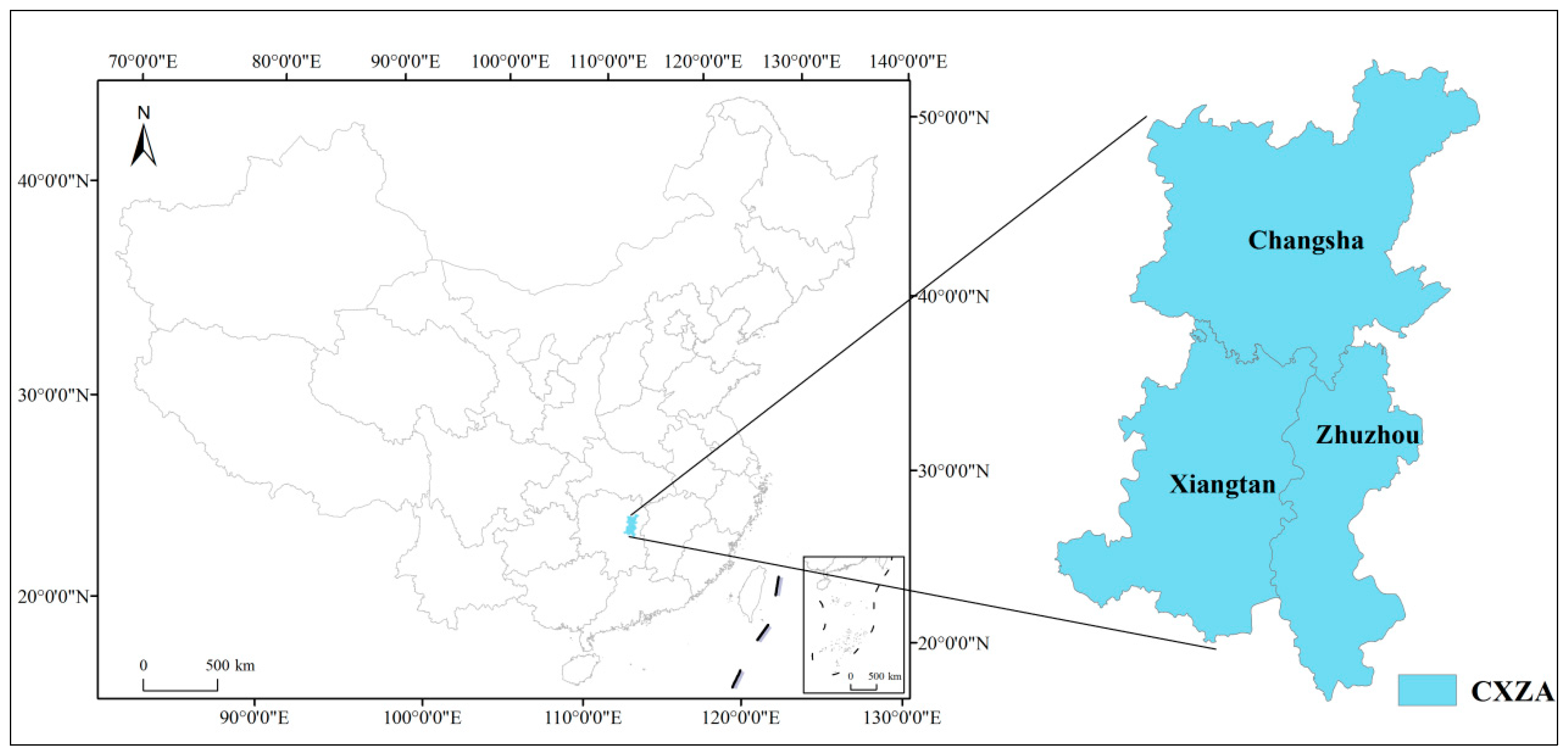
2.1. Study Area
2.2. LST Retrieval and LCZ Classification
2.2.1. Preprocessing of the Landsat Data
2.2.2. LST Retrieval and Accuracy Assessment
2.2.3. LCZ Mapping Method and Accuracy Assessment
2.3. Calculation of Parameters Affecting Thermal Environment
2.3.1. Landscape Pattern Calculation
2.3.2. Urban Volume Calculation
2.3.3. Urban Morphology Calculation
2.4. Statistical Analysis
2.5. Cooling Model Construction
3. Results
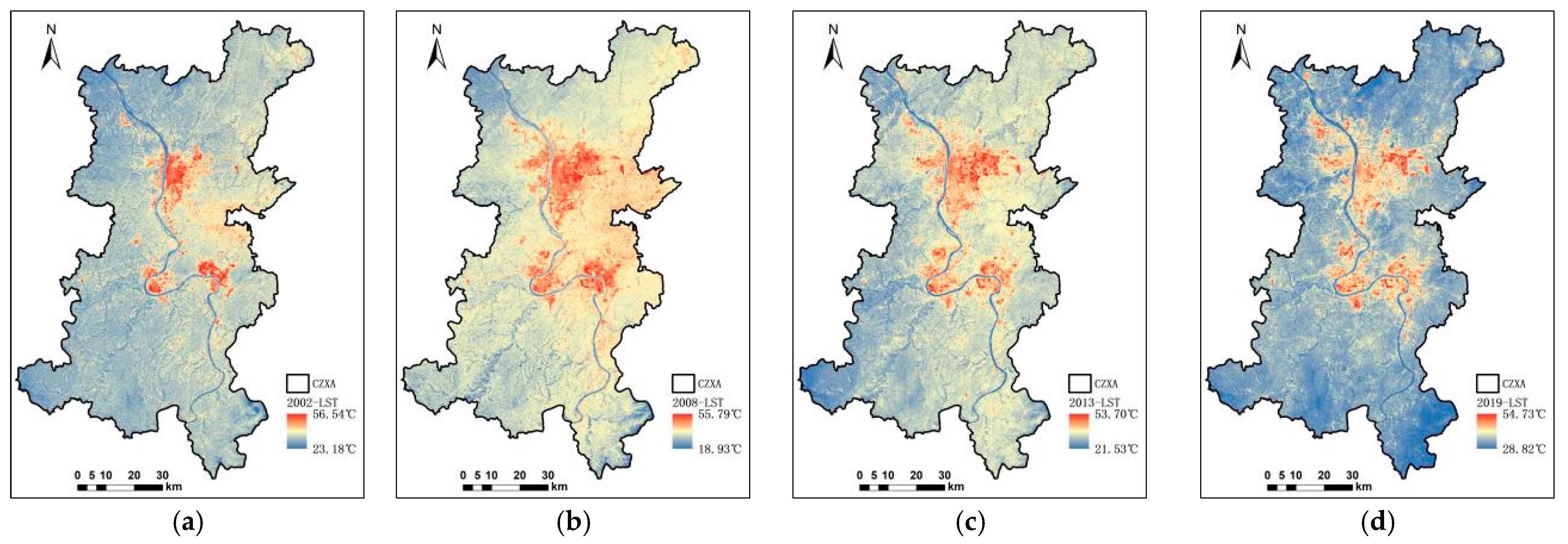
3.1. Spatial–Temporal Distributions of LCZs and LST
3.2. Correlation Between Urban Thermal Environment and Different Aspects Factors
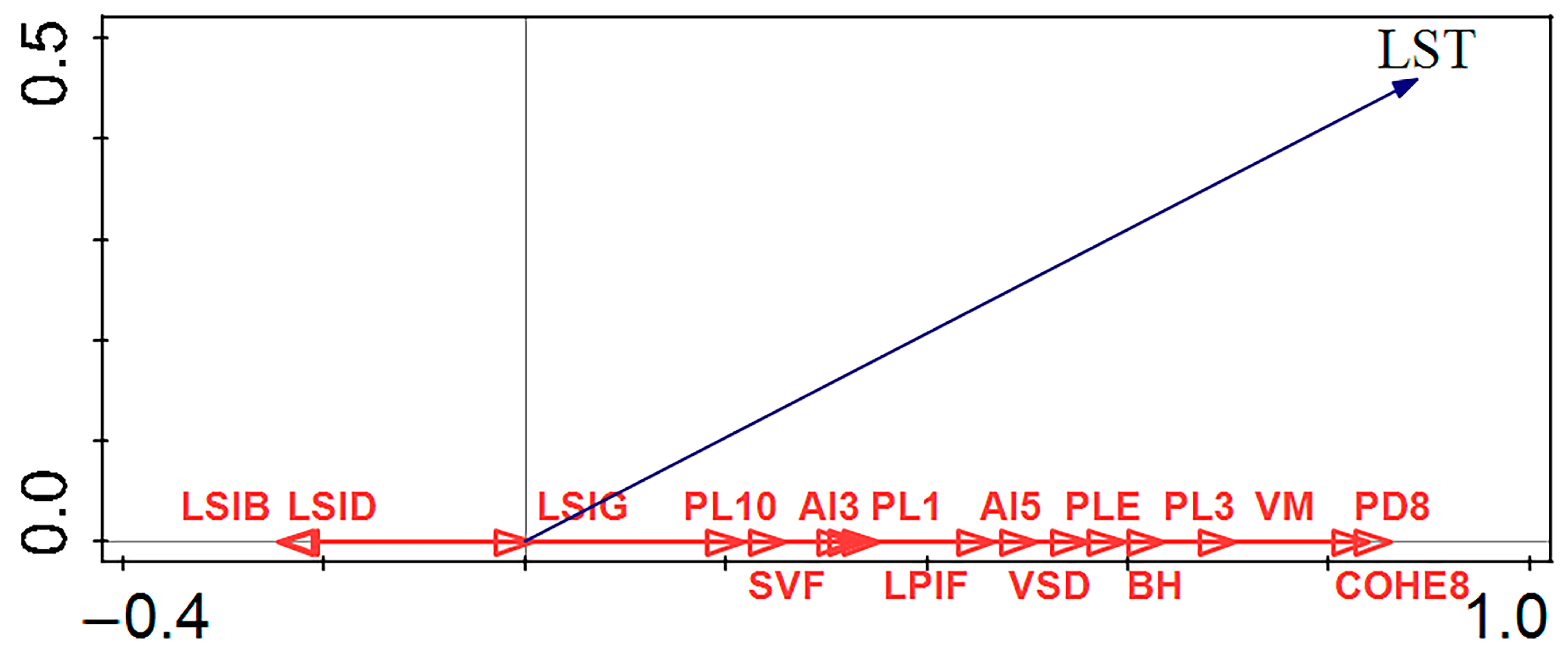
3.3. Redundancy Analysis Results
3.4. Cooling Model
4. Discussion
4.1. Analysis of Influence Mechanism of Urban Thermal Environment
4.2. Key Parameters Affecting Thermal Environment
4.3. Cooling Suggestions Based on Cooling Model
5. Conclusions
Author Contributions
Funding
Data Availability Statement
Acknowledgments
Conflicts of Interest
Appendix A


| LCZ_1: Compact high-rise | LCZ_2: Compact mid-rise | LCZ_3: Compact low-rise |
|
|
|
 |  |  |
| LCZ_4: Open high-rise | LCZ_5: Open mid-rise | LCZ_6: Open low-rise |
|
|
|
 |  |  |
| LCZ_8: Large low-rise | LCZ_9: Sparsely built | LCZ_10: Heavy industry |
|
|
|
 |  |  |
| LCZ_A: Dense trees | LCZ_B: Scattered trees | LCZ_D: Low plants |
|
|
|
 |  |  |
| LCZ_E: Bare rock or paved | LCZ_F: Bare soil or sand | LCZ_G: Water |
|
|
|
 |  |  |
| Years | Site Name | Longitude (Degree Minutes) | Latitude (Degree Minutes) | Measured Temperature/°C | Retrieved LST/℃ | Errors/°C |
|---|---|---|---|---|---|---|
| 17 August 2019 at 10:57 a.m. | Changsha | 11,255 | 2813 | 33.60 | 33.26 | −0.34 |
| Zhuzhou | 11,310 | 2752 | 33.90 | 35.03 | 1.13 | |
| Xiangtan | 11,249 | 2752 | 34.30 | 35.04 | 0.74 | |
| Mapoling | 11,247 | 2807 | 34.20 | 34.66 | 0.46 | |
| 17 September 2013 at 10:59 a.m. | Changsha | 11,255 | 2813 | 33.20 | 32.03 | −1.17 |
| Zhuzhou | 11,310 | 2752 | 32.20 | 33.48 | 1.28 | |
| Xiangtan | 11,249 | 2752 | 32.20 | 32.29 | 0.09 |
| The Accuracy of the New Samples | The Accuracy of GLC_FCS30 | |||||
|---|---|---|---|---|---|---|
| Years of New Samples | Overall Accuracy | Kappa Coefficient | Years of LCZs | Years of GLC_FCS30 | Overall Accuracy | Kappa Coefficient |
| 2002 | 77.30% | 0.70 | 2002 | 2000 | 71.19% | 0.70 |
| 2008 | 81.83% | 0.74 | 2002 | 2005 | 71.58% | 0.70 |
| 2013 | 77.27% | 0.72 | 2008 | 2010 | 75.30% | 0.62 |
| 2019 | 83.10% | 0.77 | 2013 | 2015 | 73.33% | 0.72 |
| 2019 | 2020 | 74.78% | 0.74 | |||
| Years | DF | Sig = 0 | LCZ Pairs with Insignificant Differences |
|---|---|---|---|
| 2002 | 14 | LCZ_2 and LCZ_1, LCZ_3 and LCZ_1, LCZ_4 and LCZ_1, LCZ_5 and LCZ_1, LCZ_6 and LCZ_1, LCZ_8 and LCZ_1, LCZ_8 and LCZ_4, LCZ_10 and LCZ_1, LCZ_10 and LCZ_3, LCZ_E and LCZ_1, LCZ_F and LCZ_1 | 11/105 |
| 2008 | 14 | LCZ_5 and LCZ_1, LCZ_E and LCZ_8, LCZ_F and LCZ_1 | 3/105 |
| 2013 | 14 | LCZ_6 and LCZ_4, LCZ_10 and LCZ_2, LCZ_B and LCZ_9, LCZ_E and LCZ_1 | 4/105 |
| 2019 | 14 | LCZ_10 and LCZ_1, LCZ_E and LCZ_1, LCZ_E and LCZ_10 | 3/105 |
| Criterion Layer | Parameters | Data Sources | Preprocessing |
|---|---|---|---|
| Socioeconomic Development | Population Density | Resource and Environment Science and Data Center | Projection Transformation, Downsampling |
| Gross Domestic Product (GDP) Density | Projection Transformation, Downsampling | ||
| 2.5-micrometer Particulate Matter (PM2.5) Concentration | China High Air Pollutants (CHAP) | Panoply, ArcGIS, Inverse Distance Weight (IDW), Projection Transformation, Resampling | |
| Physical Geography | Elevation | USGS-SRTM | Projection Transformation, Downsampling |
| Slope | USGS-SRTM | ArcGIS, Slope Calculation Tool | |
| Vegetation Coverage | Landsat imagery | Threshold segmentation with NDVI | |
| Urban Construction | COHESION8 | Conclusion of the previous article | RDA analysis |
| VM | |||
| PD8 | |||
| Land Use Barrier | Distribution of each LCZ | Conclusion of the previous article | The standard deviation level method |
| No | Data List | The Role of Data |
|---|---|---|
| 1 | Landsat5 | LCZ classification, LST retrieval |
| 2 | Landsat8 | |
| 3 | Temperature recorded at the station | LST accuracy assessment |
| 4 | Google Earth historical images | LCZ mapping |
| 5 | Field research data | |
| 6 | Baidu Street View | |
| 7 | Anjuke | |
| 8 | GLC_FCS30 | LCZ accuracy assessment |
| 9 | Landscape metric | Landscape pattern calculation |
| 10 | ZY-3 satellite data | Urban volume calculation |
| 11 | ALOS satellite data | |
| 12 | OSM data | Urban morphology calculation |
| 13 | DSM data | |
| 14 | Remote sensing data | |
| 15 | Population Density | Cooling model construction |
| 16 | GDP | |
| 17 | PM2.5 | |
| 18 | Elevation | |
| 19 | Slope | |
| 20 | Vegetation Coverage |
| No | Term | Full English Name |
|---|---|---|
| 1 | AI | Aggregation Index |
| 2 | ANOVA | One-Way Analysis of Variance |
| 3 | BH | Building Height |
| 4 | BSF | Building Surface Fraction |
| 5 | CFC | CF_Central |
| 6 | CHAP | China High Air Pollutants |
| 7 | COHESION | Patch Cohesion Index |
| 8 | CONTAG | Contagion Index |
| 9 | DEM | Digital Elevation Model |
| 10 | DSM | Digital Surface Model |
| 11 | GDP | Gross Domestic Product |
| 12 | GI | Green Infrastructure |
| 13 | GLC_FCS30 | Global Land-cover Product with Fine Classification System at 30 m |
| 14 | GM | Gravity Model |
| 15 | H/W | Height Width Ratio |
| 16 | ISF | Impervious Surface Fraction |
| 17 | LCZ | Local Climate Zones |
| 18 | LPI | Largest Patch Index |
| 19 | LSI | Landscape Shape Index |
| 20 | LST | Land Surface Temperature |
| 21 | MCR | Minimum Cumulative Resistance Mode |
| 22 | NDBI | Normalized Difference Built-up Index |
| 23 | NDVI | Normalized Difference Vegetation Index |
| 24 | OA | Overall Accuracy |
| 25 | OSM | Open Street Map |
| 26 | PD | Patch Density |
| 27 | PLAND | Percentage of Landscape |
| 28 | PM 2.5 | 2.5-micrometer Particulate Matter |
| 29 | PSF | Pervious Surface Fraction |
| 30 | RDA | Redundancy Analysis |
| 31 | RF | Random Forest |
| 32 | RS | Remote Sensing |
| 33 | RTE | Radiative Transfer Equation |
| 34 | SHDI | Shannon’s Diversity Index |
| 35 | SLR | Stepwise linear regression |
| 36 | SPCA | Spatial Principal Component Analysis |
| 37 | SVF | Sky View Factor |
| 38 | SW | Mean Street Width |
| 39 | Tukey’s HSD | Tukey’s Honest Significant Difference |
| 40 | UCZ | Urban Climate Zone |
| 41 | UHI | Urban Heat Island |
| 42 | UTZ | Urban Terrain Zone |
| 43 | VM | Volume Mean |
| 44 | VSD | Volume Standard Deviation |
| 45 | WUDAPT | The World Urban Database and Portal Tools |
References
- Cano, D.; Cacciuttolo, C.; Rosario, C.; Barzola, R.; Pizarro, S.; Ramirez, D.W.; Freitas, M.; Bremer, U.F. Performance of Green Areas in Mitigating the Alteration of Land Surface Temperature in Urban Zones of Lima, Peru. Remote Sens. 2025, 17, 1323. [Google Scholar] [CrossRef]
- Wang, J.; Lu, L.; Zhou, X.; Huang, G.; Chen, Z. Spatio-Temporal Patterns and Drivers of the Urban Heat Island Effect in Arid and Semi-Arid Regions of Northern China. Remote Sens. 2025, 17, 1339. [Google Scholar] [CrossRef]
- Bao, Y.; Du, H.; Huang, Z.; Ren, S.; Yin, G.; Mao, R. Assessing and mitigating the carbon emissions from illegal urban buildings: A spatial lifecycle analysis. Resour. Conserv. Recycl. 2025, 215, 108097. [Google Scholar] [CrossRef]
- Schneider, A.; Friedl, M.A.; Potere, D. Mapping global urban areas using MODIS 500-m data: New methods and datasets based on ‘urban ecoregions’. Remote Sens. Environ. 2010, 114, 1733–1746. [Google Scholar] [CrossRef]
- Yinghui, C.; Xiaomin, G. Disparities in the impact of urban heat island effect on particulate pollutants at different pollution stages—A case study of the “2 + 36” cities. Urban Clim. 2025, 59, 102273. [Google Scholar] [CrossRef]
- Wu, T.; Wu, S.; Hu, S.; Zhang, Q. Simulating future cultivated land using a localized SSPs-RCPs framework: A case study in Yangtze River Economic Belt. Habitat Int. 2024, 154, 103210. [Google Scholar] [CrossRef]
- Hua, S.; Jing, H.; Yao, Y.; Guo, Z.; Lerner, D.N.; Andrews, C.B.; Zheng, C. Can groundwater be protected from the pressure of China’s urban growth? Environ. Int. 2020, 143, 105911. [Google Scholar] [CrossRef]
- Zhan, X.; Liang, D.; Lin, X.; Li, L.; Wei, C.; Dingle, C.; Liu, Y. Background noise but not urbanization level impacted song frequencies in an urban songbird in the Pearl River Delta, Southern China. Glob. Ecol. Conserv. 2021, 28, e01695. [Google Scholar] [CrossRef]
- Oukawa, G.Y.; Krecl, P.; Targino, A.C. Fine-scale modeling of the urban heat island: A comparison of multiple linear regression and random forest approaches. Sci. Total Environ. 2022, 815, 152836. [Google Scholar] [CrossRef]
- Huang, Q. Effects of urban spatial morphology on urban heat island effect from multi-spatial scales perspectives. Sci. Geogr. Sin. 2021, 41, 1832–1842. [Google Scholar]
- Peng, J.; Ma, J.; Liu, Q.; Liu, Y.; Hu, Y.; Li, Y.; Yue, Y. Spatial-temporal change of land surface temperature across 285 cities in China: An urban-rural contrast perspective. Sci. Total Environ. 2018, 635, 487–497. [Google Scholar] [CrossRef] [PubMed]
- Ejaz, F.; Kausar, A.; Maqsoom, A.; Khan, O.I.; Lahori, A.H. Spatio-temporal analysis of Karachi metropolitan as an urban heat island. Adv. Space Res. 2025, 75, 331–352. [Google Scholar] [CrossRef]
- Zhao, Y.; Chen, Y.; Li, K. Revealing the impacts of 3D urban morphology on surface temperature considering geometry heterogeneity, component contribution, and scale effect. Sustain. Cities Soc. 2025, 119, 106093. [Google Scholar] [CrossRef]
- Zuo, W.; Ren, Z.; Shan, X.; Zhou, Z.; Deng, Q.; Bonafoni, S. Analysis of Urban Heat Island Effect in Wuhan Urban Area Based on Prediction of Urban Underlying Surface Coverage Type Change. Adv. Meteorol. 2024, 2024, 4509221. [Google Scholar] [CrossRef]
- Luo, T.; Jia, J.; Qiu, Y.; Zhang, Y. Effects of Urban Tree Species and Morphological Characteristics on the Thermal Environment: A Case Study in Fuzhou, China. Forests 2024, 15, 2075. [Google Scholar] [CrossRef]
- Li, X.; Liu, S.; Ma, Q.; Cao, W.; Zhang, H.; Wang, Z. Impacts of spatial explanatory variables on surface urban heat island intensity between urban and suburban regions in China. Int. J. Digit. Earth 2024, 17, 2304074. [Google Scholar] [CrossRef]
- Hashim, B.M.; Al Maliki, A.; Sultan, M.A.; Shahid, S.; Yaseen, Z.M. Effect of land use land cover changes on land surface temperature during 1984–2020: A case study of Baghdad city using landsat image. Nat. Hazards 2022, 112, 1223–1246. [Google Scholar] [CrossRef]
- Wu, Q.; Li, Z.Y.; Yang, C.B.; Li, H.Q.; Gong, L.W.; Guo, F.X. On the Scale Effect of Relationship Identification between Land Surface Temperature and 3D Landscape Pattern: The Application of Random Forest. Remote Sens. 2022, 14, 279. [Google Scholar] [CrossRef]
- Xiong, L.W.; Li, S.X.; Zou, B.; Peng, F.; Fang, X.; Xue, Y. Long Time-Series Urban Heat Island Monitoring and Driving Factors Analysis Using Remote Sensing and Geodetector. Front. Environ. Sci. 2022, 9, 828230. [Google Scholar] [CrossRef]
- Cai, Z.; Han, G.; Chen, M. Do water bodies play an important role in the relationship between urban form and land surface temperature? Sustain. Cities Soc. 2018, 39, 487–498. [Google Scholar] [CrossRef]
- Wang, Y. The Coolong Effect of Urban Waterbody Landscape: Case Study of Wuhan. Ph.D. Thesis, Wuhan University, Wuhan, China, 2019. [Google Scholar]
- Arnfield, A.J. Two decades of urban climate research: A review of turbulence, exchanges of energy and water, and the urban heat island. Int. J. Climatol. 2003, 23, 1–26. [Google Scholar] [CrossRef]
- Theeuwes, N.E.; Steeneveld, G.J.; Ronda, R.J.; Heusinkveld, B.G.; van Hove, L.W.A.; Holtslag, A.A.M. Seasonal dependence of the urban heat island on the street canyon aspect ratio. Q. J. R. Meteorol. Soc. 2014, 140, 2197–2210. [Google Scholar] [CrossRef]
- Marciotto, E.R.; Oliveira, A.P.; Hanna, S.R. Modeling study of the aspect ratio influence on urban canopy energy fluxes with a modified wall-canyon energy budget scheme. Build. Environ. 2010, 45, 2497–2505. [Google Scholar] [CrossRef]
- Chen, L.; Yang, J.; Zheng, X. Modelling the impact of building energy consumption on urban thermal environment: The bias of the inventory approach. Urban Clim. 2024, 53, 101802. [Google Scholar] [CrossRef]
- Lin, P.; Lau, S.S.Y.; Qin, H.; Gou, Z. Effects of urban planning indicators on urban heat island: A case study of pocket parks in high-rise high-density environment. Landsc. Urban Plan. 2017, 168, 48–60. [Google Scholar] [CrossRef]
- Mi, X.; Bai, L.; Zhao, Y. Analysis of urban heat island effect in Taiyuan based on multi source satellite data. Sci. Technol. Eng. 2021, 21, 13650–13658. [Google Scholar]
- Wang, Q. Study on the Spatio-Space Dirtribution of Urban Heat Island Effect in Changchun City Based on Remote Sensing Technology. Master’s Thesis, Changchun Institute of Technology, Changchun, China, 2019. [Google Scholar]
- Houet, T.; Pigeon, G. Mapping urban climate zones and quantifying climate behaviors—An application on Toulouse urban area (France). Environ. Pollut. 2011, 159, 2180–2192. [Google Scholar] [CrossRef]
- Stewart, I.D.; Oke, T.R. Local Climate Zones for Urban Temperature Studies. Bull. Am. Meteorol. Soc. 2012, 93, 1879–1900. [Google Scholar] [CrossRef]
- Bechtel, B.; Alexander, P.; Böhner, J.; Ching, J.; Conrad, O.; Feddema, J.; Mills, G.; See, L.; Stewart, I. Mapping Local Climate Zones for a Worldwide Database of the Form and Function of Cities. ISPRS Int. J. Geo-Inf. 2015, 4, 199–219. [Google Scholar] [CrossRef]
- Baqa, M.F.; Lu, L.; Guo, H.; Song, X.; Alavipanah, S.K.; Nawaz-ul-Huda, S.; Li, Q.; Chen, F. Investigating heat-related health risks related to local climate zones using SDGSAT-1 high-resolution thermal infrared imagery in an arid megacity. Int. J. Appl. Earth Obs. Geoinf. 2025, 136, 104334. [Google Scholar] [CrossRef]
- Aslam, A.; Rana, I.A.; Bhatti, S.S. Local climate zones and its potential for building urban resilience: A case study of Lahore, Pakistan. Int. J. Disaster Resil. Built Environ. 2022, 13, 248–265. [Google Scholar] [CrossRef]
- Cai, M.; Ren, C.; Xu, Y.; Lau, K.K.; Wang, R. Investigating the relationship between local climate zone and land surface temperature using an improved WUDAPT methodology—A case study of Yangtze River Delta, China. Urban Clim. 2018, 24, 485–502. [Google Scholar] [CrossRef]
- Zhang, R.; Chen, T.; Su, F.; Liu, Y.; Zheng, G. Simulating the Impact of Urban Expansion on Ecological Security Pattern from a Multi-Scenario Perspective: A Case Changsha–Zhuzhou–Xiangtan Urban Agglomeration, China. Sustainability 2024, 16, 9382. [Google Scholar] [CrossRef]
- Huang, X.; Xie, Y.; Lei, F.; Cao, L.; Zeng, H. Analysis on spatio-temporal evolution and influencing factors of ecosystem service in the Changsha-Zhuzhou-Xiangtan urban agglomeration, China. Front. Environ. Sci. 2024, 11, 1334458. [Google Scholar] [CrossRef]
- Duan, S.; Ru, C.; Li, Z. Reviews of methods for land surface temperature retrieval from Landsat thermal infrared data. Natl. Remote Sens. Bull. 2021, 25, 1591–1617. [Google Scholar] [CrossRef]
- Sobrino, J.A.; Jiménez-Muñoz, J.C.; Paolini, L. Land surface temperature retrieval from LANDSAT TM 5. Remote Sens. Environ. 2004, 90, 434–440. [Google Scholar] [CrossRef]
- Zhang, X.; Liu, L.; Chen, X.; Gao, Y.; Xie, S.; Mi, J. GLC_FCS30: Global land-cover product with fine classification system at 30 m using time-series Landsat imagery. Earth Syst. Sci. Data 2021, 13, 2753–2776. [Google Scholar] [CrossRef]
- Gao, Y.; Liu, L.; Zhang, X.; Chen, X.; Mi, J.; Xie, S. Consistency Analysis and Accuracy Assessment of Three Global 30-m Land-Cover Products over the European Union using the LUCAS Dataset. Remote Sens. 2020, 12, 3479. [Google Scholar] [CrossRef]
- Li, P.; Wang, Y.; Wang, C.; Tian, L.; Lin, M.; Xu, S.; Zhu, C. A Comparison of Recent Global Time-Series Land Cover Products. Remote Sens. 2025, 17, 1417. [Google Scholar] [CrossRef]
- Danylo, O.; See, L.; Bechtel, B.; Schepaschenko, D.; Fritz, S. Contributing to WUDAPT: A Local Climate Zone Classification of Two Cities in Ukraine. IEEE J. Sel. Top. Appl. Earth Observ. Remote Sens. 2016, 9, 1841–1853. [Google Scholar] [CrossRef]
- Unal Cilek, M.; Cilek, A. Analyses of land surface temperature (LST) variability among local climate zones (LCZs) comparing Landsat-8 and ENVI-met model data. Sustain. Cities Soc. 2021, 69, 102877. [Google Scholar] [CrossRef]
- Ge, M.; Fang, S.; Gong, Y.; Tao, P.; Yang, G.; Gong, W. Understanding the Correlation between Landscape Pattern and Vertical Urban Volume by Time-Series Remote Sensing Data: A Case Study of Melbourne. ISPRS Int. J. Geo-Inf. 2021, 10, 14. [Google Scholar] [CrossRef]
- Feng, B.; Yang, H.; Ren, Y.; Zheng, S.; Feng, G.; Huang, Y. Study on Change of Landscape Pattern Characteristics of Comprehensive Land Improvement Based on Optimal Spatial Scale. Land 2025, 14, 135. [Google Scholar] [CrossRef]
- Luo, J.; Fan, Y.; Wu, H.; Cheng, J.; Yang, R.; Zheng, K. Quantifying the Spatial Distribution Pattern of Soil Diversity in Southern Xinjiang and Its Influencing Factors. Sustainability 2024, 16, 2561. [Google Scholar] [CrossRef]
- Li, B.; Zhang, Y.; Gan, T. Temporal and Spatial Changes of Landscape Pattern of Changsha, Zhuzhou and Xiangtan Urban Agglomeration. Chin. Overseas Archit. 2018, 11, 57–61. [Google Scholar]
- Wang, J.; Zhan, Q.M.; Guo, H.G.; Jin, Z.C. Characterizing the spatial dynamics of land surface temperature–impervious surface fraction relationship. Int. J. Appl. Earth Obs. Geoinf. 2016, 45, 55–65. [Google Scholar] [CrossRef]
- Wang, H.; Sun, S.; Wang, B.; Song, F. Analysis of Similarities and Differences between DEM and DSM Data in Production and Application. Geomat. Spat. Inf. Technol. 2018, 41, 156–158. [Google Scholar]
- Zhang, Q.; Yang, Q.; Cheng, J.; Wang, C. Characteristics of 3′′ SRTM Errors in China. Geomat. Inf. Sci. Wuhan Univ. 2018, 43, 684–690. [Google Scholar]
- Scarano, M.; Mancini, F. Assessing the relationship between sky view factor and land surface temperature to the spatial resolution. Int. J. Remote Sens. 2017, 38, 6910–6929. [Google Scholar] [CrossRef]
- Dozier, J.; Bruno, J. A faster solution to the horizon problem. Comput. Geosci. 1981, 7, 145–151. [Google Scholar] [CrossRef]
- Zakšek, K.; Oštir, K.; Kokalj, Ž. Sky-View Factor as a Relief Visualization Technique. Remote Sens. 2011, 3, 398–415. [Google Scholar] [CrossRef]
- Qiao, Z.; Jia, R.; Liu, J.; Gao, H.; Wei, Q. Remote Sensing-Based Analysis of Urban Heat Island Driving Factors: A Local Climate Zone Perspective. IEEE J. Sel. Top. Appl. Earth Observ. Remote Sens. 2024, 17, 17337–17348. [Google Scholar] [CrossRef]
- Qin, M.; Ouyang, H.; Jiang, H.; Luo, T.; Zhou, Y.; Liu, Y. Spatiotemporal evolution characteristics and driving factors of heat island effect based on territorial perspective: A case study of Beibu Gulf urban agglomeration, China. Ecol. Indic. 2024, 166, 112197. [Google Scholar] [CrossRef]
- Lv, D.; Cai, H.; Zhang, X. Construction and optimization of the ecological security pattern in Yiyang County based on the remote sensing ecological index. Res. Agric. Mod. 2021, 42, 545–556. [Google Scholar]
- Cheng, Z.; He, Q. Remote Sensing Evaluation of the Ecological Environment of Su-Xi-Chang City Group based on Remote Sensing Ecological Index (RSEI). Remote Sens. Technol. Appl. 2019, 34, 531–539. [Google Scholar]
- Forman, R.T.T. Some general principles of landscape and regional ecology. Landsc. Ecol. 1995, 10, 133–142. [Google Scholar] [CrossRef]
- Wu, J.; He, H.; Hu, T. Analysis of factors influencing the “source-sink” landscape contribution of land surface temperature. Acta Geogr. Sin. 2022, 77, 51–65. [Google Scholar]
- Li, Y.; Sun, Y.; Li, J. Socioeconomic drivers of urban heat island effect Empirical evidence from major Chinese cities. Sustain. Cities Soc. 2020, 63, 102425. [Google Scholar] [CrossRef]
- Yao, L.; Sun, S.; Song, C.; Li, J.; Xu, W.; Xu, Y. Understanding the spatiotemporal pattern of the urban heat island footprint in the context of urbanization, a case study in Beijing, China. Appl. Geogr. 2021, 133, 102496. [Google Scholar] [CrossRef]
- Feng, Z.; Wang, X.; Yu, M.; Yuan, Y.; Li, B. PM2.5 reduces the daytime/nighttime urban heat island intensity over mainland China. Sustain. Cities Soc. 2025, 118, 106001. [Google Scholar] [CrossRef]
- Fan, S. Study on the Optimization of the Spatial Pattern of Ecological Land Use in the Beibu Gulf Urban Agglomeration Based on the Goal of Weakening the Heat Island Effect. Master’s Thesis, Guangxi University, Nanning, China, 2021. [Google Scholar]
- Liu, F.; Liu, J.; Zhang, Y.; Hong, S.; Fu, W.; Wang, M.; Dong, J. Construction of a cold island network for the urban heat island effect mitigation. Sci. Total Environ. 2024, 915, 169950. [Google Scholar] [CrossRef] [PubMed]
- Liu, Y.; Chen, H.; Wu, J.; Wang, Y.; Ni, Z.; Chen, S. Impact of urban spatial dynamics and blue-green infrastructure on urban heat islands: A case study of Guangzhou using Local Climate Zones and predictive modeling. Sustain. Cities Soc. 2024, 115, 105819. [Google Scholar] [CrossRef]
- Li, H.; Ma, T.; Wang, K. Construction of Ecological Security Pattern in Northern Peixian Based on MCR and SPCA. J. Ecol. Rural Environ. 2020, 36, 1036–1045. [Google Scholar]
- Guo, N.; Liang, X. Robustness assessment of urban cold island network based on green infrastructure—A case study of Bengbu, China. Ecol. Indic. 2024, 169, 112842. [Google Scholar] [CrossRef]
- Cao, Y.; Yang, R.; Carver, S. Linking wilderness mapping and connectivity modelling: A methodological framework for wildland network planning. Biol. Conserv. 2020, 251, 108679. [Google Scholar] [CrossRef]
- Adriaensen, F.; Chardon, J.P.; De Blust, G.; Swinnen, E.; Villalba, S.; Gulinck, H.; Matthysen, E. The application of ‘least-cost’ modelling as a functional landscape model. Landsc. Urban Plan. 2003, 64, 233–247. [Google Scholar] [CrossRef]
- Dickson, B.G.; Albano, C.M.; Anantharaman, R.; Beier, P.; Fargione, J.; Graves, T.A.; Gray, M.E.; Hall, K.R.; Lawler, J.J.; Leonard, P.B.; et al. Circuit-theory applications to connectivity science and conservation. Conserv. Biol. 2018, 33, 239–249. [Google Scholar] [CrossRef]
- Yang, W.; Yu, K.; Zhao, G.; Gen, J. Optimization of greenways in Fuzhou based on heat island effect. J. Zhejiang A&F Univ. 2022, 39, 876–883. [Google Scholar]
- Zhou, W.; Cao, F.L.; Wang, G.B. Effects of Spatial Pattern of Forest Vegetation on Urban Cooling in a Compact Megacity. Forests 2019, 10, 282. [Google Scholar] [CrossRef]
- Tang, Y.; Chen, H.; Yang, M.; Tan, Z.; Zhao, F.; Guo, J.; Fang, Y. Weak geostrophic wind driven ventilation in street canyons with trees and green walls: Cooperating or opposing dispersions of airborne pollutants? Build. Environ. 2024, 259, 111654. [Google Scholar] [CrossRef]
- Zheng, Y.; Ren, C.; Xu, Y.; Wang, R.; Ho, J.; Lau, K.; Ng, E. GIS-based mapping of Local Climate Zone in the high-density city of Hong Kong. Urban Clim. 2018, 24, 419–448. [Google Scholar] [CrossRef]
- Necira, H.; Matallah, M.E.; Bouzaher, S.; Mahar, W.A.; Ahriz, A. Effect of Street Asymmetry, Albedo, and Shading on Pedestrian Outdoor Thermal Comfort in Hot Desert Climates. Sustainability 2024, 16, 1291. [Google Scholar] [CrossRef]
- Taleghani, M.; Kleerekoper, L.; Tenpierik, M.; van den Dobbelsteen, A. Outdoor thermal comfort within five different urban forms in the Netherlands. Build. Environ. 2015, 83, 65–78. [Google Scholar] [CrossRef]
- Xi, Y.; Wang, S.; Zou, Y.; Zhou, X.; Zhang, Y. Seasonal surface urban heat island analysis based on local climate zones. Ecol. Indic. 2024, 159, 111669. [Google Scholar] [CrossRef]
- Zhu, L.; Yang, J.; Ouyang, X.; Xu, Y.; Wong, M.S.; Menenti, M. Street trees: The contribution of latent heat flux to cooling dense urban areas. Urban Clim. 2024, 58, 102147. [Google Scholar] [CrossRef]
- Wu, Q.; Huang, Y.; Irga, P.; Kumar, P.; Li, W.; Wei, W.; Shon, H.K.; Lei, C.; Zhou, J.L. Synergistic control of urban heat island and urban pollution island effects using green infrastructure. J. Environ. Manag. 2024, 370, 122985. [Google Scholar] [CrossRef]
- Hu, M.M.; Wang, Y.F.; Xia, B.C.; Huang, G.H. Surface temperature variations and their relationships with land cover in the Pearl River Delta. Environ. Sci. Pollut. Res. 2020, 27, 37614–37625. [Google Scholar] [CrossRef]
- Jinjie, D.; Liuxin, C.; Chengyun, Y.; Zhibo, X. Significance evaluation of ecological corridor in an highly-urbanized areas: A case study of Shenzhen. Geogr. Res. 2017, 36, 573–582. [Google Scholar]
- Gao, D.; Wang, Z.; Gao, X.; Chen, S.; Chen, R.; Gao, Y. Constructing an Ecological Network Based on Heat Environment Risk Assessment: An Optimisation Strategy for Thermal Comfort Coupling Society and Ecology. Sustainability 2024, 16, 4109. [Google Scholar] [CrossRef]
- Luo, Y.; Wu, Z.; Wong, M.S.; Yang, J.; Jiao, Z. Simulating the impact of ventilation corridors for cooling air temperature in local climate zone scheme. Sustain. Cities Soc. 2024, 115, 105848. [Google Scholar] [CrossRef]
- Salvati, A.; Kolokotroni, M. Urban microclimate and climate change impact on the thermal performance and ventilation of multi-family residential buildings. Energy Build. 2023, 294, 113224. [Google Scholar] [CrossRef]


| Data | Resolution | Path/Row | Date |
|---|---|---|---|
| Landsat5 | Multispectral 30 m, Thermal Infrared 120 m. | 123/40 123/41 | 3 September 2002 at 10:31 a.m. |
| 19 September 2008 at 10:41 a.m. | |||
| Landsat8 | Multispectral 30 m, Thermal Infrared 100 m. | 17 September 2013 at 10:59 a.m. | |
| 17 August 2019 at 10:57 a.m. |
| Morphologies | Definition | Data Source | Calculation Formula | Parameter Definition |
|---|---|---|---|---|
| SVF | The ratio of sky hemisphere visible from the ground | DSM | λi is the height angle between observation point i and surrounding buildings. n is the number of horizon search directions. | |
| BH | Mean building height of an LCZ grid | Building data | n is the number of buildings of the LCZ sample site. BSi is the ground area of a building. BHi is the height of a building. | |
| BSF | The fraction of land surface covered by buildings | Building data | BSi is the ground area of a building. Ssite is the area of the LCZ sample site. | |
| SW | Mean street width of an LCZ grid | Street data | Sstreet is the total area of the LCZ sample site. SLi is the total length of the LCZ sample site. | |
| H/W | The ratio of height to width of a street canyon | Building and street data | is the mean building height of an LCZ grid. SW is the mean street width of an LCZ grid. | |
| PSF | Pervious surface fraction of the LCZ sample site | Remote sensing data | Sper is the area of pervious surface of the LCZ sample site. Ssite is the area of the LCZ sample site. | |
| ISF | Impervious surface fraction of the LCZ sample site | Remote sensing data |
| Fragmentation | ||||||||
|---|---|---|---|---|---|---|---|---|
| Years | PD | PD1 | PD2 | PD3 | PD4 | PD5 | PD6 | PD8 |
| 2002 | 0.47 ** | 0.04 ** | 0.39 ** | 0.33 ** | 0.31 ** | 0.47 ** | 0.46 ** | 0.42 ** |
| 2008 | 0.42 ** | 0.20 ** | 0.54 ** | 0.46 ** | 0.47 ** | 0.55 | 0.51 ** | 0.52 ** |
| 2013 | 0.59 ** | 0.28 ** | 0.64 ** | 0.54 ** | 0.48 ** | 0.33 ** | 0.52 ** | 0.66 ** |
| 2019 | 0.68 ** | 0.35 ** | 0.74 ** | 0.61 ** | 0.66 ** | 0.64 ** | 0.55 ** | 0.74 ** |
| Years | PD9 | PD10 | PDA | PDB | PDD | PDE | PDG | |
| 2002 | −0.20 ** | 0.33 ** | −0.19 ** | 0.23 ** | 0.09 ** | 0.39 ** | 0.42 ** | 0.24 ** |
| 2008 | −0.21 ** | 0.26 ** | −0.22 ** | −0.15 ** | −0.04 ** | 0.43 ** | 0.40 ** | 0.06 ** |
| 2013 | 0.03 ** | 0.29 ** | −0.14 ** | −0.08 ** | −0.31 ** | 0.55 ** | 0.46 ** | −0.07 ** |
| 2019 | 0.08 ** | 0.32 ** | −0.23 ** | −0.20 ** | −0.16 | 0.60 ** | 0.38 ** | 0.00 ** |
| Years | PL1 | PL2 | PL3 | PL4 | PL5 | PL6 | PL8 | PL9 |
| 2002 | 0.04 ** | 0.27 ** | 0.25 ** | 0.30 ** | 0.45 ** | 0.40 ** | 0.35 ** | −0.08 ** |
| 2008 | 0.16 ** | 0.48 ** | 0.39 ** | 0.40 ** | 0.52 ** | 0.54 ** | 0.52 ** | −0.01 ** |
| 2013 | 0.24 ** | 0.56 ** | 0.49 ** | 0.48 ** | 0.38 ** | 0.56 ** | 0.68 ** | −0.09 ** |
| 2019 | 0.28 ** | 0.65 ** | 0.56 ** | 0.64 ** | 0.60 ** | 0.53 ** | 0.79 ** | −0.15 ** |
| Years | PL10 | PLA | PLB | PLD | PLE | PLF | PLG | |
| 2002 | 0.28 ** | −0.38 ** | 0.15 ** | 0.05 ** | 0.33 ** | 0.33 ** | 0.07 ** | |
| 2008 | 0.26 ** | −0.18 ** | 0.00 ** | 0.12 ** | 0.43 ** | 0.42 ** | 0.19 ** | |
| 2013 | 0.20 ** | −0.29 ** | −0.06 ** | −0.42 ** | 0.51 ** | 0.39 ** | −0.21 ** | |
| 2019 | 0.23 ** | −0.54 ** | −0.16 ** | −0.23 ** | 0.53 ** | 0.33 ** | −0.09 ** | |
| Years | LPI | LPI1 | LPI2 | LPI3 | LPI4 | LPI5 | LPI6 | LPI8 |
| 2002 | −0.24 ** | 0.09 ** | 0.38 ** | 0.33 ** | 0.39 ** | 0.52 ** | 0.44 ** | 0.42 ** |
| 2008 | −0.24 ** | 0.05 ** | 0.29 ** | 0.26 ** | 0.32 ** | 0.39 ** | 0.38 ** | 0.38 ** |
| 2013 | −0.35 ** | 0.27 ** | 0.48 ** | 0.46 ** | 0.41 ** | 0.35 ** | 0.47 ** | 0.60 ** |
| 2019 | −0.52 ** | 0.32 ** | 0.59 ** | 0.57 ** | 0.65 ** | 0.53 ** | 0.45 ** | 0.70 ** |
| Years | LPI9 | LPI10 | LPIA | LPIB | LPID | LPIE | LPIF | LPIG |
| 2002 | 0.02 ** | 0.33 ** | −0.19 ** | −0.08 ** | −0.24 ** | 0.36 ** | 0.32 ** | −0.15 ** |
| 2008 | 0.06 ** | 0.26 ** | −0.20 ** | 0.00 ** | −0.22 ** | 0.36 ** | 0.35 ** | −0.16 ** |
| 2013 | −0.06 ** | 0.18 ** | −0.26 ** | −0.05 ** | −0.39 ** | 0.49 ** | 0.34 ** | −0.20 ** |
| 2019 | −0.14 ** | 0.22 ** | −0.50 ** | −0.15 ** | −0.22 ** | 0.48 ** | 0.31 ** | −0.09 ** |
| Complexity | ||||||||
| Years | LSI | LSI1 | LSI2 | LSI3 | LSI4 | LSI5 | LSI6 | LSI8 |
| 2002 | 0.36 ** | 0.08 ** | 0.58 ** | 0.50 ** | 0.40 ** | 0.41 ** | 0.52 ** | 0.56 ** |
| 2008 | 0.30 ** | 0.21 ** | 0.55 ** | 0.48 ** | 0.49 ** | 0.54 ** | 0.52 ** | 0.50 ** |
| 2013 | 0.45 ** | 0.31 ** | 0.64 ** | 0.58 ** | 0.45 ** | 0.29 ** | 0.49 ** | 0.66 ** |
| 2019 | 0.56 ** | 0.39 ** | 0.76 ** | 0.64 ** | 0.58 ** | 0.63 ** | 0.56 ** | 0.78 ** |
| Years | LSI9 | LSI10 | LSIA | LSIB | LSID | LSIE | LSIF | LSIG |
| 2002 | −0.29 ** | 0.47 ** | −0.20 ** | 0.00 ** | −0.07 ** | 0.50 ** | 0.44 ** | 0.02 ** |
| 2008 | −0.22 ** | 0.29 ** | −0.33 ** | −0.14 ** | −0.17 ** | 0.45 ** | 0.42 ** | 0.06 ** |
| 2013 | −0.15 ** | 0.30 ** | −0.27 ** | −0.09 ** | −0.43 ** | 0.56 ** | 0.46 ** | −0.08 ** |
| 2019 | −0.07 ** | 0.34 ** | −0.43 ** | −0.22 ** | −0.22 ** | 0.62 ** | 0.40 ** | 0.00 ** |
| Aggregation | ||||||||
| Years | AI | AI1 | AI2 | AI3 | AI4 | AI5 | AI6 | AI8 |
| 2002 | −0.35 ** | 0.00 ** | 0.43 ** | 0.37 ** | 0.16 ** | 0.38 ** | 0.32 ** | 0.37 ** |
| 2008 | −0.29 ** | 0.11 ** | 0.41 ** | 0.40 ** | 0.35 ** | 0.43 ** | 0.43 ** | 0.39 ** |
| 2013 | −0.43 ** | 0.13 ** | 0.45 ** | 0.38 ** | 0.31 ** | 0.24 ** | 0.34 ** | 0.54 ** |
| 2019 | −0.54 ** | 0.16 ** | 0.51 ** | 0.30 ** | 0.46 ** | 0.41 ** | 0.30 ** | 0.65 ** |
| Years | AI9 | AI10 | AIA | AIB | AID | AIE | AIF | AIG |
| 2002 | −0.06 ** | 0.30 ** | −0.19 ** | −0.03 ** | −0.22 ** | 0.26 ** | 0.32 ** | −0.05 ** |
| 2008 | 0.03 ** | 0.13 ** | −0.31 ** | −0.12 ** | −0.31 ** | 0.23 ** | 0.35 ** | −0.07 ** |
| 2013 | −0.05 ** | 0.14 ** | −0.28 ** | −0.03 ** | −0.40 ** | 0.30 ** | 0.37 ** | −0.11 ** |
| 2019 | −0.11 ** | 0.14 ** | −0.49 ** | −0.11 ** | −0.21 ** | 0.28 ** | 0.34 ** | −0.03 ** |
| Years | CO | CO1 | CO2 | CO3 | CO4 | CO5 | CO6 | CO8 |
| 2002 | −0.40 ** | 0.00 ** | 0.48 ** | 0.39 ** | 0.20 ** | 0.52 ** | 0.43 ** | 0.45 ** |
| 2008 | −0.38 ** | 0.13 ** | 0.46 ** | 0.42 ** | 0.39 ** | 0.50 ** | 0.51 ** | 0.48 ** |
| 2013 | −0.55 ** | 0.17 ** | 0.54 ** | 0.44 ** | 0.42 ** | 0.36 ** | 0.49 ** | 0.66 ** |
| 2019 | −0.64 ** | 0.19 ** | 0.60 ** | 0.37 ** | 0.60 ** | 0.55 ** | 0.44 ** | 0.77 ** |
| Years | CO9 | CO10 | COA | COB | COD | COE | COF | COG |
| 2002 | −0.13 ** | 0.33 ** | −0.19 ** | −0.06 ** | −0.22 ** | 0.28 ** | 0.35 ** | −0.07 ** |
| 2008 | −0.05 ** | 0.15 ** | −0.31 ** | −0.16 ** | −0.31 ** | 0.27 ** | 0.38 ** | −0.09 ** |
| 2013 | −0.14 ** | 0.17 ** | −0.31 ** | −0.05 ** | −0.42 ** | 0.36 ** | 0.40 ** | −0.14 ** |
| 2019 | −0.16 ** | 0.16 ** | −0.53 ** | −0.13 ** | −0.24 ** | 0.37 ** | 0.35 ** | −0.04 ** |
| Aggregation | Diversity | |||||||
| Years | CONTAG | Years | SHDI | |||||
| 2002 | −0.13 ** | 2002 | 0.41 ** | |||||
| 2008 | −0.09 ** | 2008 | 0.37 ** | |||||
| 2013 | −0.39 ** | 2013 | 0.54 ** | |||||
| 2019 | −0.50 ** | 2019 | 0.66 ** | |||||
| Urban Volume Metrics | Mean (m3) | Regression Equations with LST | R2 | Pearson |
|---|---|---|---|---|
| VM | 14031 | 0.40 ** | 0.63 | |
| VSD | 18659 | 0.21 ** | 0.46 |
| Urban Morphologies | Regression Equations with LST | R2 | Pearson |
|---|---|---|---|
| SVF | 0.00 ** | 0.20 | |
| BH | 0.25 ** | 0.50 | |
| BSF | 0.31 ** | 0.55 | |
| SW | 0.44 ** | 0.66 | |
| H/W | 0.02 ** | 0.15 | |
| PSF | 0.68 ** | −0.82 | |
| ISF | 0.68 ** | 0.82 |
| No. | Metrics | Standardized Coefficient | Tolerance | VIF |
|---|---|---|---|---|
| 1 | PLAND1 | 0.044 ** | 0.449 | 2.229 |
| 2 | AI1 | 0.011 ** | 0.671 | 1.49 |
| 3 | PLAND3 | 0.046 ** | 0.32 | 3.128 |
| 4 | AI3 | −0.012 ** | 0.699 | 1.431 |
| 5 | AI5 | −0.015 ** | 0.515 | 1.941 |
| 6 | PD8 | 0.057 ** | 0.204 | 4.905 |
| 7 | COHE8 | −0.044 ** | 0.116 | 8.616 |
| 8 | AI9 | 0.048 ** | 0.123 | 8.159 |
| 9 | PLAND10 | 0.045 ** | 0.752 | 1.33 |
| 10 | LSIB | 0.069 ** | 0.361 | 2.767 |
| 11 | LSID | −0.093 ** | 0.227 | 4.401 |
| 12 | PLANDE | 0.044 ** | 0.524 | 1.907 |
| 13 | LPIF | 0.035 ** | 0.393 | 2.544 |
| 14 | LSIG | 0.041 ** | 0.461 | 2.169 |
| 15 | VM | 0.104 ** | 0.126 | 7.966 |
| 16 | VSD | −0.078 ** | 0.193 | 5.176 |
| 17 | SVF | 0.111 ** | 0.211 | 4.749 |
| 18 | BH | −0.059 ** | 0.273 | 3.665 |
| Goodness | R2 | 0.885 | ||
| Cooling Sources | Extremely Important | Important | Generally Important | Cooling Corridors | Extremely Important | Important | Generally Important | Cooling Nodes | Primary | Secondary | Tertiary |
|---|---|---|---|---|---|---|---|---|---|---|---|
| Number | 16 | 17 | 17 | Number | 46 | 46 | 47 | Number | 27 | 26 | 15 |
| Area | 1233.30 | 407.08 | 495.76 | Total Length | 418.04 | 805.11 | 135.88 | ||||
| Area Ratio | 57.73 | 19.06 | 23.21 | Average Length | 8.89 | 17.50 | 29.41 | ||||
| Length Ratio | 16.23 | 31.25 | 52.52 | ||||||||
Disclaimer/Publisher’s Note: The statements, opinions and data contained in all publications are solely those of the individual author(s) and contributor(s) and not of MDPI and/or the editor(s). MDPI and/or the editor(s) disclaim responsibility for any injury to people or property resulting from any ideas, methods, instructions or products referred to in the content. |
© 2025 by the authors. Licensee MDPI, Basel, Switzerland. This article is an open access article distributed under the terms and conditions of the Creative Commons Attribution (CC BY) license (https://creativecommons.org/licenses/by/4.0/).
Share and Cite
Ge, M.; Xiong, Z.; Li, Y.; Li, L.; Xie, F.; Gong, Y.; Sun, Y. Research on Thermal Environment Influencing Mechanism and Cooling Model Based on Local Climate Zones: A Case Study of the Changsha–Zhuzhou–Xiangtan Urban Agglomeration. Remote Sens. 2025, 17, 2391. https://doi.org/10.3390/rs17142391
Ge M, Xiong Z, Li Y, Li L, Xie F, Gong Y, Sun Y. Research on Thermal Environment Influencing Mechanism and Cooling Model Based on Local Climate Zones: A Case Study of the Changsha–Zhuzhou–Xiangtan Urban Agglomeration. Remote Sensing. 2025; 17(14):2391. https://doi.org/10.3390/rs17142391
Chicago/Turabian StyleGe, Mengyu, Zhongzhao Xiong, Yuanjin Li, Li Li, Fei Xie, Yuanfu Gong, and Yufeng Sun. 2025. "Research on Thermal Environment Influencing Mechanism and Cooling Model Based on Local Climate Zones: A Case Study of the Changsha–Zhuzhou–Xiangtan Urban Agglomeration" Remote Sensing 17, no. 14: 2391. https://doi.org/10.3390/rs17142391
APA StyleGe, M., Xiong, Z., Li, Y., Li, L., Xie, F., Gong, Y., & Sun, Y. (2025). Research on Thermal Environment Influencing Mechanism and Cooling Model Based on Local Climate Zones: A Case Study of the Changsha–Zhuzhou–Xiangtan Urban Agglomeration. Remote Sensing, 17(14), 2391. https://doi.org/10.3390/rs17142391