Abstract
Very high resolution (VHR) remote sensing change detection (CD) is crucial for monitoring Earth’s dynamics but faces challenges in capturing fine-grained changes and distinguishing them from pseudo-changes due to varying acquisition conditions. Existing deep learning methods often suffer from information loss via downsampling, obscuring details, and lack filter adaptability to spatial heterogeneity. To address these issues, we introduce Information-Preserving Adaptive Convolutional Network (IPACN). IPACN features a novel Information-Preserving Backbone (IPB), leveraging principles adapted from reversible networks to minimize feature degradation during hierarchical bi-temporal feature extraction, enhancing the preservation of fine spatial details, essential for accurate change delineation. Crucially, IPACN incorporates a Frequency-Adaptive Difference Enhancement Module (FADEM) that applies adaptive filtering, informed by frequency analysis concepts, directly to the bi-temporal difference features. The FADEM dynamically refines change signals based on local spectral characteristics, improving discrimination. This synergistic approach, combining high-fidelity feature preservation (IPB) with adaptive difference refinement (FADEM), yields robust change representations. Comprehensive experiments on benchmark datasets demonstrate that IPACN achieves state-of-the-art performance, showing significant improvements in F1 score and IoU, enhanced boundary delineation, and improved robustness against pseudo-changes, offering an effective solution for very high resolution remote sensing CD.
1. Introduction
Remote sensing change detection (CD), the process of identifying differences in the Earth’s surface state from multi-temporal observations, plays a fundamental role across diverse domains, including environmental monitoring, urban development tracking, agricultural management, and disaster impact assessment [1,2]. The proliferation of very high resolution (VHR) satellite and aerial imagery offers unprecedented spatial detail, enabling the analysis of fine-scale changes, critical for many applications [1]. However, this increased resolution also presents significant challenges for automated analysis, demanding sophisticated algorithms capable of handling intricate details and complex scenes [3,4].
Despite considerable advancements driven by deep learning (DL), achieving accurate and robust CD in VHR images remains a complex task [5,6]. Several key challenges remain: (1) Loss of fine-grained information: Standard DL architectures often employ downsampling operations (e.g., pooling, strided convolutions) to build hierarchical representations and increase receptive fields. While effective for capturing semantics, this process inherently leads to a loss of fine spatial details [7,8], a problem that is particularly detrimental in VHR CD. It hinders the ability to detect subtle changes, accurately delineate complex or irregular change boundaries, and distinguish small objects [9], which are fundamental tasks in high-resolution earth observation. (2) Pseudo-change interference: VHR images are highly sensitive to variations in acquisition conditions unrelated to actual land cover changes. Differences in illumination, atmospheric conditions, seasonality, sensor calibration, and minor misregistration can introduce significant pixel-level differences, known as pseudo-changes, which are easily misinterpreted as genuine changes [10,11]. Distinguishing these artifacts from true changes is a major hurdle. (3) Scene heterogeneity and filter inflexibility: Remote sensing scenes exhibit high spatial heterogeneity. Conventional convolutional filters, being static and spatially invariant, struggle to adapt their behavior to this local variability, limiting their effectiveness in optimally representing diverse features or change types [12,13].
Current DL-based CD methods, predominantly relying on convolutional neural networks (CNNs) [14,15] or Transformers [16,17], partially address these issues but retain limitations. CNN hierarchies often conflict with the need for detail preservation demanded by CD, contrasting with the information bottleneck principle [7,18]. Transformers excel at global context but can be computationally demanding and lack precise localization [19]. Crucially, these methods often struggle to simultaneouslypreserve detailed spatial information throughout the feature extraction process and adaptively process the critical bi-temporal difference features to distinguish true changes from complex pseudo-changes and noise.
Addressing these intertwined challenges necessitates a framework that synergistically combines high-fidelity feature preservation with adaptive difference signal enhancement. To this end, we introduce the Information-Preserving Adaptive Convolutional Network (IPACN). IPACN integrates two core components that are specifically re-engineered for change detection:
- An Information-Preserving Backbone (IPB): To combat information loss, the IPB leverages principles adapted from reversible networks [7,20]. Its multi-column, reversibly connected architecture facilitates quasi-lossless feature propagation, enhancing the preservation of fine spatial details critical for accurate change delineation. This provides high-quality features for subsequent difference analysis.
- A Frequency-Adaptive Difference Enhancement Module (FADEM): To tackle pseudo-changes and heterogeneity, the FADEM applies adaptive filtering, informed by frequency analysis concepts [12], directly to the bi-temporal difference features derived from the IPB. The FADEM dynamically adjusts its spatial context aggregation and kernel frequency response based on the local spectral characteristics of the difference map, allowing it to selectively enhance salient change signals while suppressing noise and pseudo-changes.
The central hypothesis of IPACN is that the high-fidelity features from the IPB provide a superior foundation for the FADEM, enabling more effective and robust refinement of change information than is possible with features from conventional, lossy backbones.
The primary contributions of this work are summarized as follows:
- The proposal of IPACN, a novel framework synergistically integrating information preservation and frequency-adaptive difference enhancement specifically for VHR remote sensing CD.
- The design and adaptation of an Information-Preserving Backbone (IPB) based on reversible network principles, tailored for extracting high-fidelity bi-temporal features in the CD context.
- The development of the Frequency-Adaptive Difference Enhancement Module (FADEM), which innovatively applies and adapts frequency-aware processing concepts to robustly refine bi-temporal difference features.
- Comprehensive experimental validation on four challenging benchmark datasets, demonstrating that IPACN achieves state-of-the-art performance compared to existing methods.
The remainder of this paper is organized as follows: Section 2 provides a review of related work. Section 3 details the proposed IPACN architecture and its components. Section 4 presents the experimental setup, results, and detailed analyses, including ablation studies. Section 5 discusses the findings, limitations, and potential future directions. Finally, Section 6 concludes the paper.
2. Related Work
Deep learning (DL) has become the dominant paradigm for remote sensing change detection (CD), significantly improving performance over traditional methods [5,6]. Early DL approaches primarily adapted segmentation architectures like fully convolutional networks (FCNs) and U-Net variants into Siamese structures for bi-temporal feature extraction and comparison [8,14,15]. While effective, these CNN-based methods inherently struggle with the progressive loss of fine spatial details due to repeated downsampling operations, compromising the precise localization needed for VHR CD [7]. Furthermore, the static nature of standard convolutional filters limits their adaptability to the diverse spectral and textural characteristics within heterogeneous VHR scenes [12].
To address the limitations of CNNs in capturing global context, Transformer architectures [16,17,21,22], leveraging self-attention, have been introduced to CD [19,22]. Transformers excel at modeling long-range dependencies but can be computationally demanding and may lack the inductive biases beneficial for precise spatial localization, often necessitating hybrid CNN-Transformer designs [19]. Despite these advancements [9], effectively minimizing information loss throughout deep feature hierarchies and adaptively processing the crucial, yet often noisy, bi-temporal difference features remain significant challenges.
Mitigating information loss is critical for preserving the fine details vital in VHR CD. While skip connections [23] and attention mechanisms [24] offer improvements, they do not fundamentally prevent information degradation in deep layers. Information-preserving or reversible network designs [25] offer a more principled solution. Reversible Column Networks (RevCol) [7], for instance, achieve quasi-lossless feature propagation and training efficiency via parallel subnets with reversible connections. However, the direct application or specific adaptation of such principles for optimizing *bi-temporal feature extraction* within the unique context of CD requires dedicated investigation. Our work addresses this by developing the Information-Preserving Backbone (IPB), adapting reversible concepts specifically to maintain feature integrity from multi-temporal inputs for robust CD.
Complementary to feature preservation is the need for adaptive processing to handle scene heterogeneity and suppress pervasive pseudo-changes. Techniques like deformable convolution (DCN) [26] provide geometric flexibility by adapting filter sampling locations. Dynamic filtering methods [27] generate input-conditioned weights. More recently, frequency-adaptive approaches, such as Frequency-Adaptive Dilated Convolution (FADC) [12], have demonstrated effectiveness in semantic segmentation by dynamically adjusting dilation and kernel frequency responses based on local spectral content. FADC adaptively balances receptive field size and feature detail preservation. While powerful, these adaptive techniques, including FADC, have primarily targeted single-image tasks. Their specific application to enhance *bi-temporal difference features*—a domain critical for CD but uniquely susceptible to noise and pseudo-change contamination—remains underexplored. Our Frequency-Adaptive Difference Enhancement Module (FADEM) is designed precisely to fill this gap, migrating and tailoring frequency-aware adaptive processing to specifically refine difference maps, thereby improving the discrimination between true changes and spurious variations.
Therefore, IPACN is proposed to synergistically address these gaps by integrating adapted principles from reversible networks (in the IPB) for high-fidelity information preservation and from frequency-adaptive convolution (in the FADEM) for robust, targeted enhancement of difference features. Crucially, while inspired by these works, our approach introduces key architectural and training distinctions: The IPB employs a weight-shared Siamese structure with end-to-end training, and the FADEM represents a streamlined re-engineering of frequency-adaptive concepts specifically for sparse difference maps.
3. Method
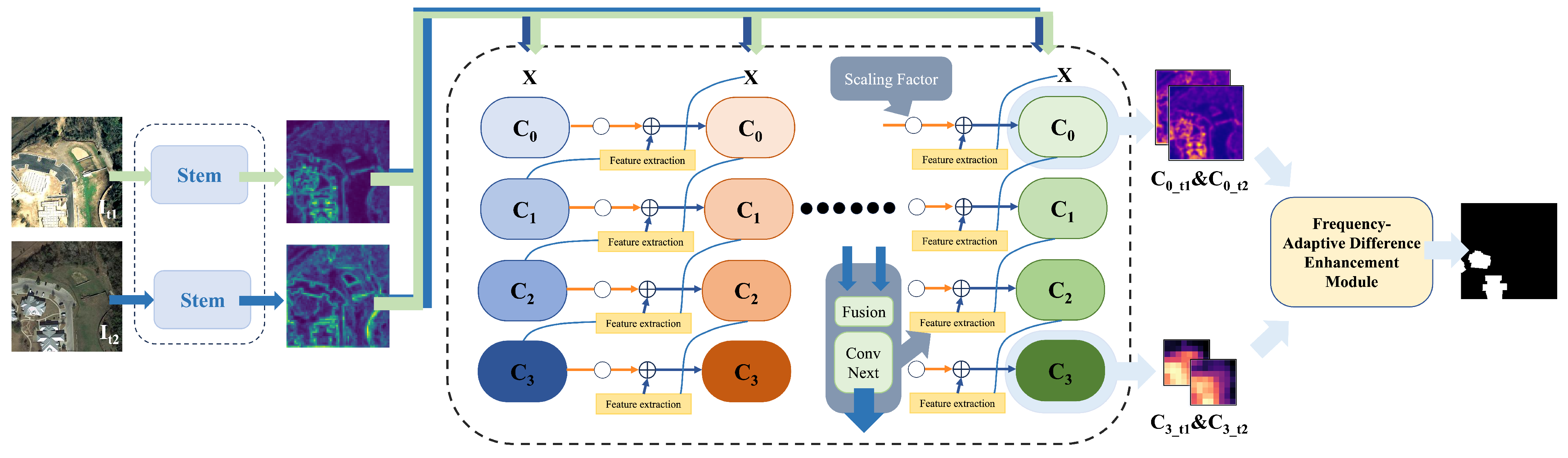
To effectively address the challenges inherent in remote sensing change detection (CD), such as the loss of critical spatial details during feature extraction, the inflexibility of standard convolutions in adapting to diverse ground features, and the susceptibility to pseudo-changes induced by varying acquisition conditions, we propose a novel deep learning framework: Information-Preserving Adaptive Convolutional Network (IPACN). This framework is meticulously engineered to generate robust and accurate change maps by synergistically integrating mechanisms for information preservation and adaptive feature processing tailored to frequency content. IPACN comprises three primary components orchestrated within a Siamese architecture: (1) a shared-weight Information-Preserving Backbone based on reversible principles, designed for quasi-lossless hierarchical feature extraction; (2) a novel Frequency-Adaptive Difference Enhancement Module (FADEM) that leverages frequency-adaptive concepts to refine bi-temporal difference features; (3) a decoder head for final change map generation. The overall workflow and architecture are depicted in Figure 1 and detailed in the subsequent sections.

Figure 1.
Overall architecture of the proposed IPACN framework. Key components include the shared Information-Preserving Backbone (IPB), temporal feature interaction, the Frequency-Adaptive Difference Enhancement Module (FADEM), and the decoder head.
3.1. Overall Architecture
The proposed Information-Preserving Adaptive Convolutional Network (IPACN) framework is illustrated in Figure 1. Designed for robust VHR change detection, IPACN processes bi-temporal images () using a Siamese architecture with a shared-weight backbone. The core workflow comprises four key stages:
- Information-Preserving Backbone (IPB): A shared backbone (detailed in Section 3.2), adapted from reversible network principles [20], extracts hierarchical feature sets and for both input images while minimizing information loss.
- Temporal feature interaction: Initial difference features are computed via absolute difference between corresponding feature levels from the two temporal branches (, primarily for and in our setup, see Section 3.3) to explicitly capture temporal discrepancies.
- Frequency-Adaptive Difference Enhancement Module (FADEM): The initial difference features from the previous step serve as the direct input to this novel module (Section 3.4). Leveraging frequency-adaptive filtering concepts [12], the FADEM processes these features to generate enhanced difference maps by adaptively refining change signals and suppressing noise.
- Decoder head: Finally, the enhanced difference features and are fed into a decoder (Section 3.5), based on the DeepLabV3+ architecture [28], which fuses the multi-level enhanced difference information to produce the final pixel-wise binary change map .
This integrated pipeline aims to deliver accurate and detailed change detection by combining high-fidelity feature preservation with adaptive difference feature refinement, as visualized in the corrected workflow in Figure 1.
3.2. Information-Preserving Backbone for Change Feature Extraction
Standard deep learning models for change detection often lose fine spatial details crucial for VHR imagery analysis due to inherent downsampling operations [8]. To address this, we designed an Information-Preserving Backbone (IPB) aimed at maximizing feature retention throughout the hierarchical extraction process, yielding high-fidelity representations, essential for accurate CD.
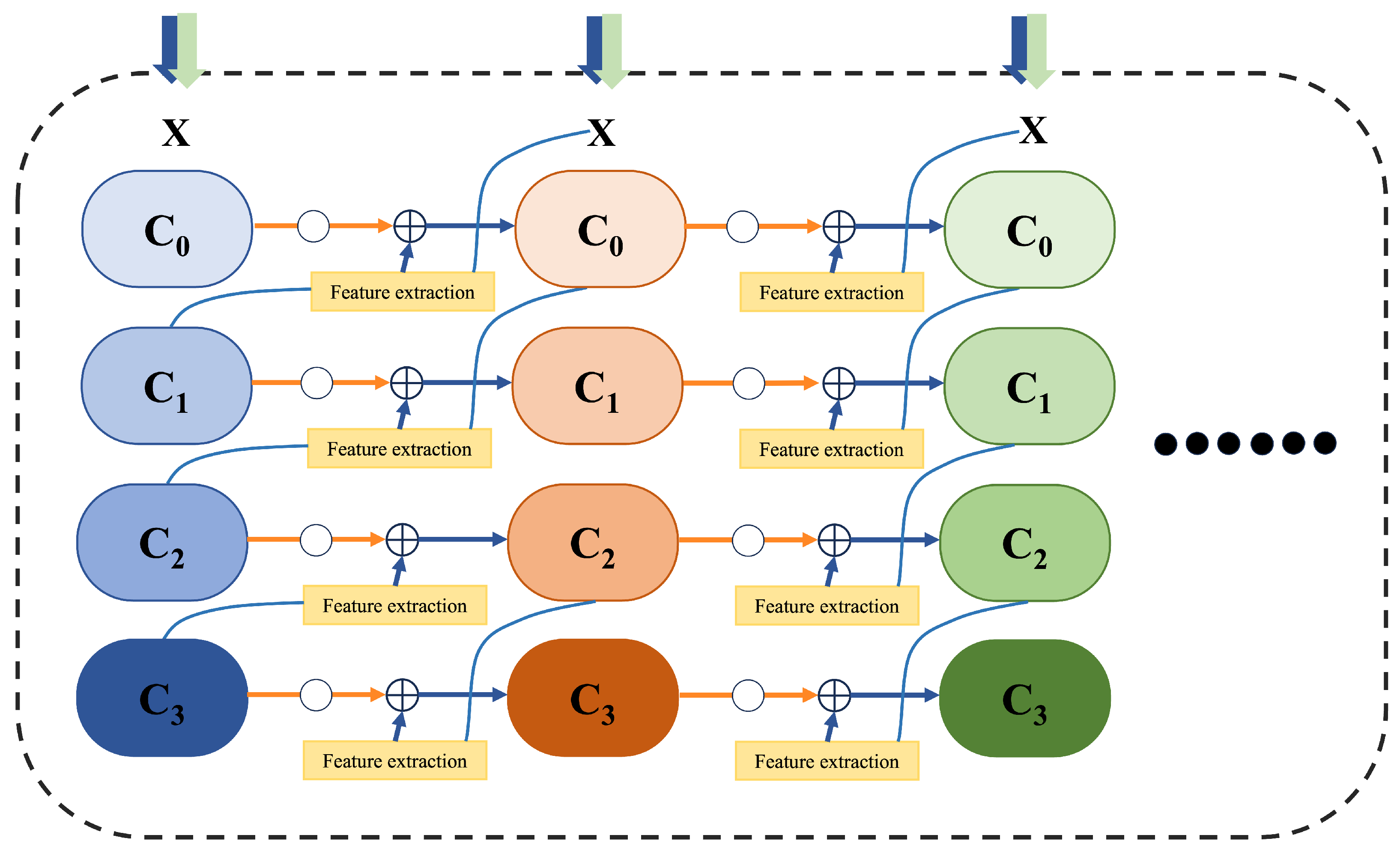
The IPB processes bi-temporal images () through a shared-weight, multi-stage architecture, depicted in Figure 1 and Figure 2. An initial stem module extracts low-level features (x). These features then pass through parallel processing columns (subnets). Each subnet refines features across four hierarchical levels (), handling progressively coarser spatial resolutions () with increasing channel depths (). This parallel, multi-level structure facilitates concurrent analysis at different scales. For our IPACN-Base model, we use , with channel depths and blocks per level. This 16-column configuration was chosen as a high-capacity setup, informed by prior work [7] that explored the trade-off between the number of columns and model performance. Empirically, it was also found to be a practical and effective scale for our computational resources, yielding strong results without incurring prohibitive training costs.

Figure 2.
Detailed conceptual architecture of the Information-Preserving Backbone (IPB). The figure illustrates the multi-column, multi-level structure where features are iteratively refined. At each level, features from the preceding column are combined with newly extracted features from the current column through additive connections (⊕), allowing for progressive information enhancement.
To maximize information preservation across the columns, the IPB utilizes specialized inter-column connections incorporating principles adapted from reversible computation [20]. This allows features to propagate through the columns with minimal loss. Within each column i () and level l, the features are computed by applying a non-linear transformation block (representing the Level module’s operations) to features from the current and preceding columns, and then integrating this output additively with a scaled representation of the features from the same level in the previous column (). This update mechanism can be conceptually represented (e.g., for level ) as
where ⊙ denotes element-wise (channel-wise) multiplication. The term is a set of learnable, channel-wise scaling factors. These factors are implemented as parameters that are specific to each level l but shared across all columns, and they are optimized via standard backpropagation along with all other network weights. The inputs to (e.g., for ) are determined by the Fusion block, combining features from different levels and columns. This additive integration, carefully managed by the learnable scaling factors, ensures effective propagation and refinement of information from earlier stages while mitigating the feature degradation common in deep sequential networks. Furthermore, a key benefit inherited from this reversible design is significantly reduced GPU memory consumption during training, as intermediate activations within the backbone can be recomputed during the backward pass instead of being stored [7,20].
The functional role of is twofold. First, as detailed in the original RevCol concept, it is critical for maintaining training stability by dynamically modulating the magnitude of the features passed through the residual connection, preventing uncontrolled growth in deep, multi-column architectures [7]. Second, its learned values provide insight into the network’s information flow patterns. For instance, if channels in learn values close to 1, it signifies that the network finds it beneficial to preserve information from the previous column almost perfectly, favoring an iterative refinement process for those feature channels. Conversely, values closer to 0 suggest that the information from the previous column is being down-weighted, with the network relying more on the new, non-linearly transformed features from the block. This channel-wise adaptive control allows the IPB to flexibly manage information propagation throughout the backbone.
Each level’s computation () is handled by a Level module (Figure 2). This module begins with a Fusion block (Figure 2), responsible for integrating appropriately downsampled features from the level below (current column) and upsampled features (via UpSampleConvnext) from the level above (previous column, except for the first column). The fused features are then refined by a sequence of ConvNextBlocks [19] utilizing efficient kernels. This standard kernel size was chosen for its computational efficiency, as we posit that the IPB’s multi-column architecture already provides a large effective receptive field through its iterative feature fusion process.
The IPB outputs two sets of high-fidelity, multi-resolution feature hierarchies, and . Unlike multi-column architectures designed for segmentation or classification tasks, that often employ intermediate supervision at various stages, our IPB is trained end-to-end, with supervision only on the final change map, allowing the entire backbone to optimize specifically for discriminative bi-temporal feature extraction. The features from levels (rich in spatial detail) and (rich in semantics), denoted and , respectively, are primarily used in the subsequent temporal feature interaction stage (Section 3.3).
3.3. Temporal Feature Interaction
Having extracted high-fidelity hierarchical features and using the shared Information-Preserving Backbone (Section 3.2), the next step is to explicitly highlight the temporal discrepancies between the two time points. We achieve this through a straightforward yet effective feature interaction mechanism. Specifically, we compute the absolute difference between the feature maps of the corresponding levels ( for high-resolution details and for semantic context) from the two temporal branches:
These resulting difference maps, and , provide initial estimates of change intensity at different feature levels. The use of absolute difference is a standard and effective technique in Siamese-based change detection frameworks to highlight temporal discrepancies while maintaining feature dimensionality [14,29]. While informative, these raw difference features may contain noise and lack the necessary refinement to reliably distinguish true changes from pseudo-changes across diverse scene complexities. Therefore, they serve as the crucial input to the subsequent enhancement stage detailed in Section 3.4.
3.4. Frequency-Adaptive Difference Enhancement Module (FADEM)
The initial difference maps (from Section 3.3) capture temporal discrepancies but often suffer from noise and fail to adequately represent the diverse characteristics of real-world changes amidst background clutter and potential pseudo-changes [13,30]. Standard static convolutional filters applied to these difference maps lack the flexibility to handle this variability effectively. To overcome this, we introduce the Frequency-Adaptive Difference Enhancement Module (FADEM), a key innovation of IPACN, designed specifically to refine these difference features by dynamically adapting its processing based on their local frequency content.
The FADEM operates on the principle that different types of change signals and noise exhibit distinct spectral characteristics. By analyzing the local frequency spectrum of the input difference map (primarily and ), the FADEM employs adaptive convolutional mechanisms to selectively enhance salient change information while suppressing irrelevant variations. This approach adapts frequency-aware processing concepts, such as those explored in FADC [12], uniquely tailoring them for the task of robust bi-temporal difference feature enhancement in remote sensing CD. Crucially, this frequency-adaptive behavior is not achieved through a separate, explicit analysis module but is an emergent property learned implicitly by the convolutional filters during end-to-end training.
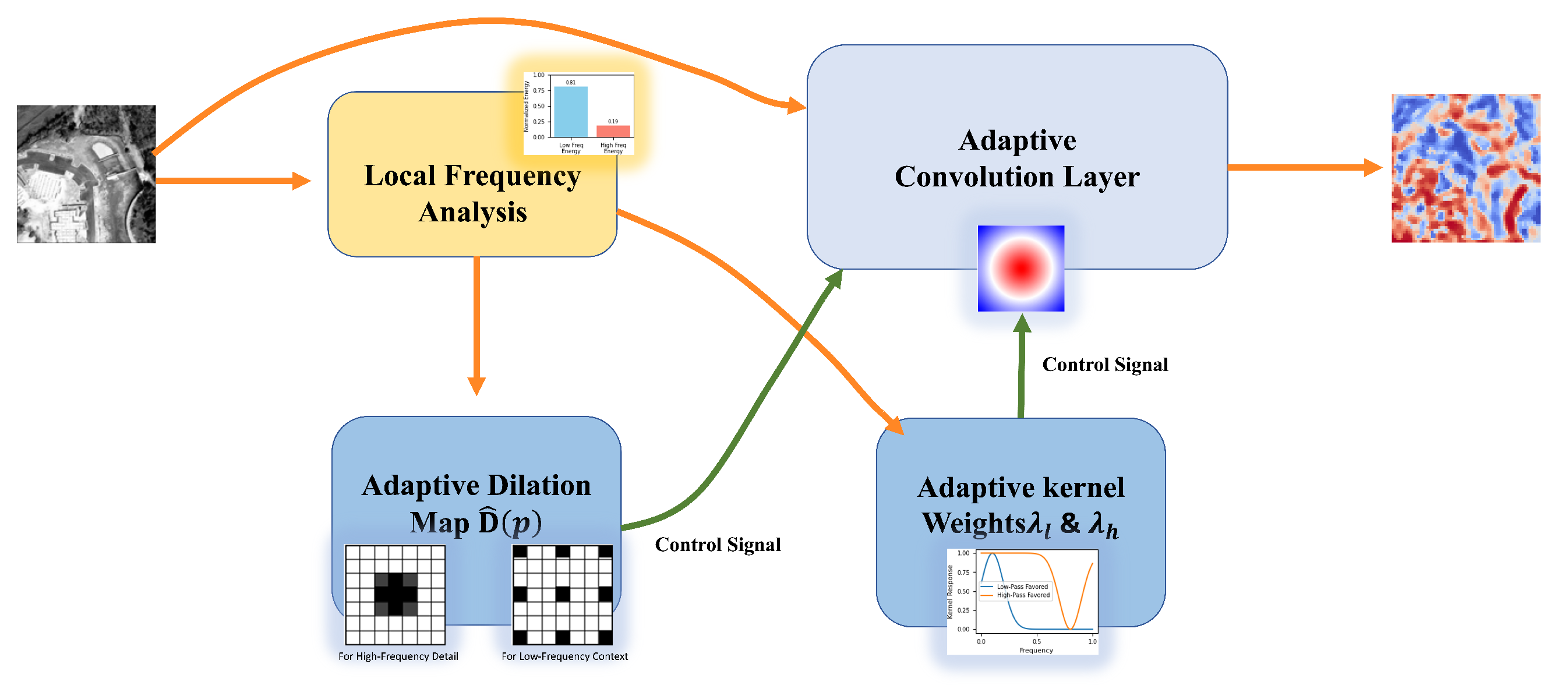
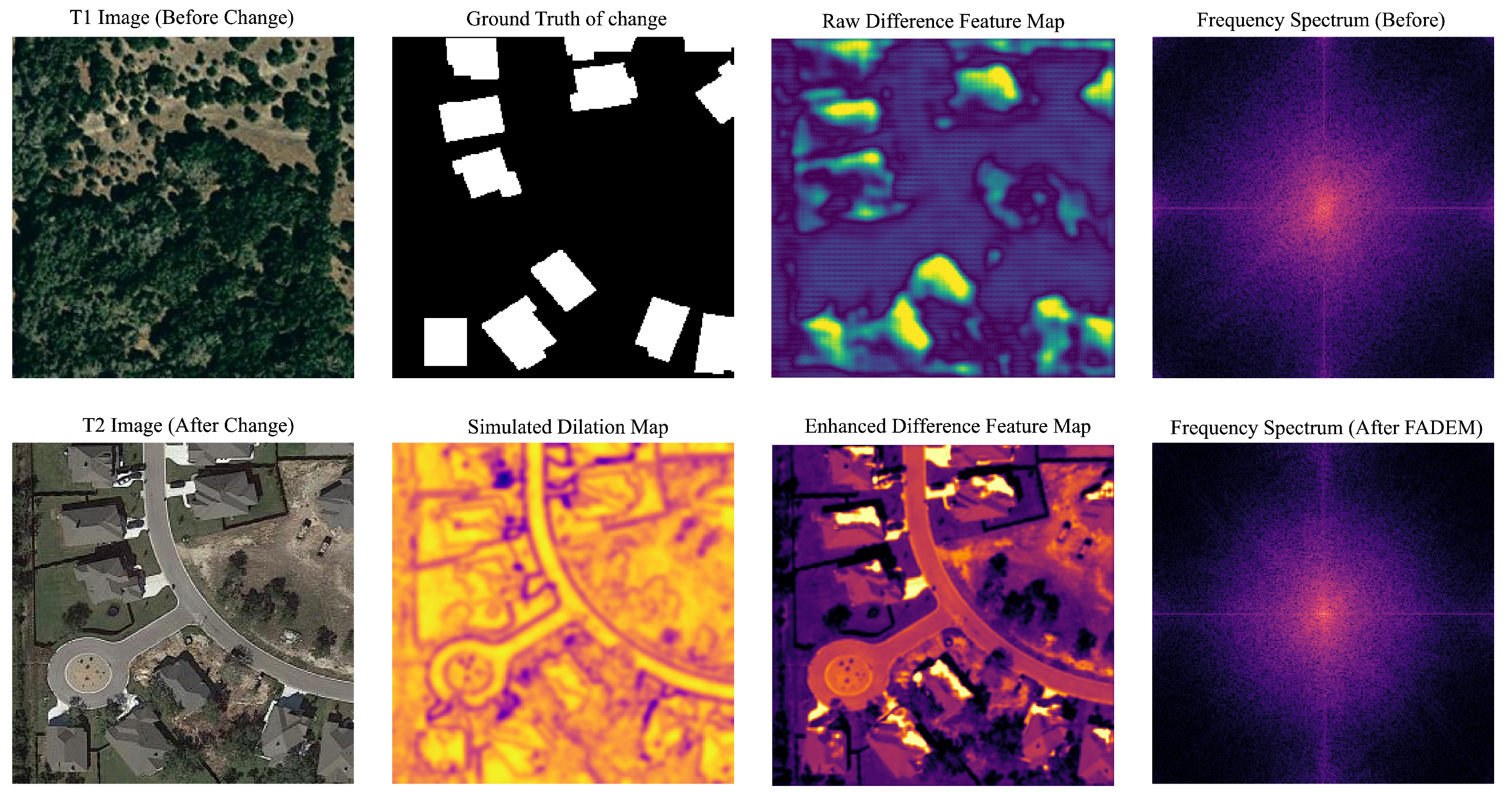
As illustrated conceptually in Figure 3, the FADEM processes each input difference map through a specialized adaptive convolution layer. To provide a concrete example of this process, a comprehensive visual analysis is presented in Figure 4. The figure demonstrates how the FADEM transforms a raw, noisy difference map into an enhanced one by modulating its frequency content. As seen in the frequency spectrum comparison within Figure 4, the FADEM effectively suppresses high-frequency noise while enhancing the signals corresponding to true changes, resulting in a cleaner and more accurate enhanced difference map. This provides direct visual evidence of the module learning a transfer function that adaptively filters the feature space. Central to this process is local frequency analysis, which examines the spectral content within local patches of . The results of this analysis generate dynamic, spatially varying control signals that govern the behavior of the convolution layer in two key ways.

Figure 3.
Conceptual illustration of the Frequency-Adaptive Difference Enhancement Module (FADEM). Input difference features () undergo analysis of local frequency content, which guides the dynamic adaptation of both spatial context aggregation (effective dilation) and filtering frequency response within the adaptive convolution layer, producing enhanced difference features (). Optional frequency-selective pre-processing may precede the adaptive convolution.

Figure 4.
Comprehensive visual analysis of the FADEM mechanism on a sample from the LEVIR-CD dataset. The top row displays: the T1 (before change) image, the ground truth mask, the initial Raw Difference Feature Map, and its corresponding frequency spectrum. The bottom row shows: the T2 (after change) image, a Simulated Dilation Map to conceptualize the adaptive process, the resulting Enhanced Difference Feature Map after FADEM processing, and its corresponding cleaned frequency spectrum. This comparison visually confirms FADEM’s ability to suppress high-frequency noise while enhancing true change signals.
- Adaptive spatial context aggregation: Based on the determined local frequency content, the FADEM dynamically adjusts its effective receptive field. For regions within rich in high-frequency components (e.g., potential change edges), the module adopts a smaller receptive field (akin to using a smaller dilation rate) to preserve fine details. Conversely, for smoother, lower-frequency regions (e.g., homogeneous areas), it expands its receptive field (akin to using a larger dilation rate) to aggregate broader context and potentially mitigate noise. This ensures the spatial context aggregation strategy matches the local characteristics of the difference signal. It is important to note that this adaptive behavior is achieved implicitly through the learned convolutional filters within the FADEM, rather than by predicting an explicit, spatially variant dilation map as in some other works [12].
- Adaptive filtering response: Concurrently, the filter’s response to different frequency components is adaptively modulated, again, guided by the local spectral analysis of . This allows the FADEM, for instance, to increase sensitivity to high-frequency components when sharp change boundaries are detected in the difference map, or to emphasize lower-frequency components when processing larger, uniform change regions. This adaptive filtering enhances the discriminability of true changes from their surrounding context and potential artifacts.
In terms of practical implementation, the FADEM is constructed from a lightweight stack of standard convolutional layers (e.g., a sequence of 3 × 3 and 1 × 1 convolutions). This design is inherently robust and does not rely on sensitive, manually tuned hyperparameters, ensuring its effectiveness and ease of use.
Optionally, prior to the adaptive convolution, a frequency-selective pre-processing step can be employed. This step could decompose into frequency bands and re-weight them using spatially varying attention, potentially suppressing high-frequency noise prevalent in difference maps or enhancing frequency ranges strongly correlated with land cover changes, yielding a pre-conditioned feature for more effective adaptive convolution.
The output of the FADEM is the enhanced difference feature map . By adaptively processing the raw differences based on their frequency content, the FADEM produces refined change representations () that are richer in relevant change information and more robust to noise and pseudo-changes, providing superior input for the final decoder head (Section 3.5). This targeted enhancement of difference features is central to IPACN’s improved performance.
3.5. Decoder Head for Change Map Generation
The enhanced difference features, (shallow-level, high-resolution details) and (deep-level, high semantics), produced by the FADEM module (Section 3.4), encapsulate the refined change information necessary for final classification. To effectively synthesize these multi-level features into a pixel-wise change map, IPACN utilizes a decoder head architecture adapted from the well-established DeepLabV3+ framework [28].
Specifically, the deep enhanced feature is first processed by an Atrous Spatial Pyramid Pooling (ASPP) module [31] to capture multi-scale context from the change representations. The resulting context-rich features are then bilinearly upsampled. Concurrently, the shallow enhanced feature undergoes channel reduction via a convolution block (self.reduce). The upsampled deep features and the processed shallow features are subsequently concatenated and fused using a sequence of convolution layers (self.fuse). Finally, a convolution (self.classifier) performs the pixel-wise classification, generating the final 2-channel logit map (), which is interpolated to the original input resolution . This process effectively combines high-level semantic change context with preserved low-level spatial details for accurate change map generation.
3.6. Loss Function for End-to-End Training
The entire IPACN, encompassing the IPB, FADEM, and decoder head, is trained end-to-end using a pixel-wise loss function suitable for binary change detection. We employ the standard binary cross-entropy (BCE) loss as the primary objective function. It is computed between the final predicted probability map (where is the sigmoid activation function applied to the logits ) and the binary ground truth change mask .The main training loss, , is the average of over all pixels in the batch.
The BCE loss for each pixel is given by
To potentially enhance gradient propagation, particularly to deeper layers, an auxiliary loss (also BCE) can be optionally computed from an intermediate feature map within the decoder (e.g., before the final classifier, after appropriate upsampling) and added to the main loss with a weighting factor :
This loss (either or ) guides the optimization of all learnable parameters throughout the IPACN framework. Notably, unlike multi-column architectures that employ intermediate supervision, our training relies solely on this final objective, allowing the entire network to optimize cohesively for change detection performance.
4. Experiments
This section details the experimental validation of the proposed IPACN framework.
4.1. Datasets
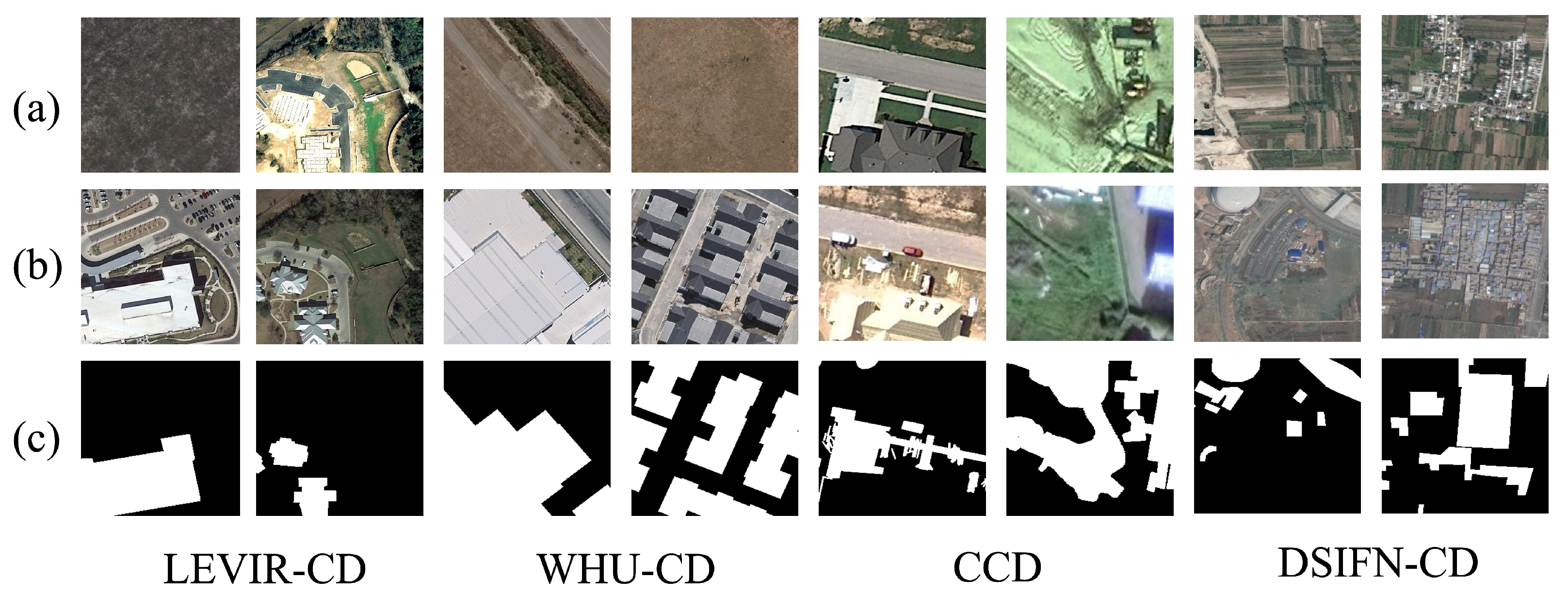
To ensure a thorough and comparable evaluation across diverse scenarios, we utilize four widely adopted public benchmark datasets for high-resolution remote sensing change detection: LEVIR-CD [29], WHU-CD [32], CDD [33], and DSIFN-CD [34]. These datasets collectively represent a variety of geographic locations, sensor characteristics, spatial resolutions, and types of land cover changes, forming a robust testbed for assessing the generalization capability and effectiveness of CD models. Example image pairs and ground truth masks illustrating the change types in each dataset are shown in Figure 5.

Figure 5.
Example image pairs (T1 images in row (a), T2 images in row (b)) and their corresponding ground truth change masks (row (c)) from four datasets: LEVIR-CD (first column), WHU-CD (second column), CCD (third column), and DSIFN-CD (fourth column).
- LEVIR-CD [29]: A large-scale dataset focusing on building changes, derived from Google Earth imagery ( m/pixel resolution) across several Texas cities. It contains 637 image pairs of size , presenting challenges related to small-object changes and complex urban contexts (see Figure 5, first column).
- WHU-CD [32]: Contains a pair of very high resolution ( m/pixel) aerial images of Christchurch, New Zealand, captured before (2012) and after (2016) significant earthquake-related reconstruction. It primarily features changes related to building construction and damage in urban and suburban areas (see Figure 5, second column).
- CDD [33]: This dataset features seasonally varying scenes from Google Earth with varying spatial resolutions ( m to m/pixel) and an image size of . It includes changes in objects like cars, roads, and buildings, testing model robustness against seasonal variations and diverse change scales (see Figure 5, third column).
- DSIFN-CD [34]: Sourced from Google Earth images of six Chinese cities, this dataset (2 m/pixel resolution, size) includes diverse land cover changes such as roads, buildings, farmland, and water bodies, offering complex multi-class change scenarios (evaluated here as binary change) (see Figure 5, fourth column).
Following standard practice for comparative studies [17], all images from these datasets were uniformly cropped into non-overlapping patches of pixels. The datasets were partitioned into training, validation, and testing sets according to the splits provided by the original authors or common benchmarks. Detailed statistics of the processed datasets are summarized in Table 1. Example image pairs and ground truth masks illustrating the change types in each dataset are shown in Figure 5.

Table 1.
Summary of the change detection datasets used in the experiments (after pre-processing into patches).
4.2. Experimental Setup and Evaluation Metrics
4.2.1. Experimental Setup
All models were implemented using the PyTorch 2.7.1 framework and trained on NVIDIA A6000 GPUs. The AdamW optimizer [35] was employed with an initial learning rate of and a weight decay of . A polynomial learning rate decay schedule (power = 0.9) was applied over 160,000 training iterations, including a linear warmup phase. For IPACN models, a layer-wise learning rate decay (decay rate: 0.9) suitable for the Information-Preserving Backbone was used. This strategy and value were adopted from the original RevCol framework [7], upon which our IPB is based, as it has been shown to be effective for stabilizing the training of deep, multi-column architectures. An effective batch size of 16 was maintained. Standard data augmentations were applied during training, including random horizontal and vertical flipping, rescaling, random cropping (), and photometric distortions. This combination of augmentations is a standard and effective practice in VHR change detection, widely adopted to enhance model generalization and prevent overfitting [17]. The same augmentation strategy was applied consistently across all datasets to ensure a fair and robust evaluation of model performance. To ensure a fair comparison and rigorously evaluate the generalization capabilities of the models, the same training configuration and hyperparameter settings were consistently applied across all four benchmark datasets. This approach minimizes dataset-specific tuning, ensuring that performance improvements can be more directly attributed to the architectural merits of the models.
4.2.2. Evaluation Metrics
To quantitatively assess the performance of the change detection models, we adopted a standard set of metrics derived from the confusion matrix based on pixel-level predictions: True positive (TP—correctly identified change pixels), false positive (FP—unchanged pixels incorrectly identified as change), true negative (TN—correctly identified unchanged pixels), and false negative (FN—change pixels incorrectly identified as unchanged). The specific metrics used are defined as follows:
- Precision (Pre): Measures the accuracy of the positive predictions (change class).
- Recall (Rec): Measures the model’s ability to identify all actual change pixels (sensitivity).
- F1 Score (F1): The harmonic mean of precision and recall, providing a balanced measure, especially useful for imbalanced datasets.
- Intersection over union (IoU): For the change class, it measures the overlap between the predicted and ground truth change regions.
- Overall accuracy (OA): The proportion of all pixels correctly classified.
Given the typical class imbalance in CD tasks, F1 and IoU are considered primary metrics for comparing model performance on the change class. OA, Pre, and Rec provide further insights into the model’s behavior.
4.3. Comparison Methods
To rigorously evaluate the proposed IPACN framework, its performance is benchmarked against a selection of representative and state-of-the-art (SOTA) change detection methods from the existing literature. The selection aims to cover different architectural paradigms and aligns closely with methods evaluated in comparable studies on the chosen benchmark datasets [22], ensuring a relevant comparison context. The methods included for comparison are as follows.
- CNN-based methods:
Foundational fully convolutional approaches.
- FC-EF [14]: Employs early fusion of bi-temporal inputs.
- FC-Siam-Di [14]: A Siamese network utilizing feature differencing.
- FC-Siam-Conc [14]: A Siamese network using feature concatenation.
- Attention-augmented CNN methods:
Architectures enhancing CNNs with attention mechanisms.
- DTCDSCN [36]: Features a dual-task constrained network incorporating attention.
- STANet [29]: Integrates specific spatial–temporal attention modules.
- IFNet [34]: Uses attention within a deeply supervised fusion framework.
- SNUNet [15]: Combines Siamese NestedUNet with channel attention.
- Transformer-based methods:
Approaches leveraging Transformer architectures for contextual modeling.
- BIT [16]: A bi-temporal image Transformer network combined with a CNN backbone.
- ChangeFormer [17]: Employs a hierarchical Transformer encoder and MLP decoder.
- Variants of our proposed method:
- IPACN-Base: Our core Information-Preserving Backbone (IPB) with simple difference features fed to the decoder, isolating the backbone’s impact.
- IPACN (Full): The complete framework, utilizing the IPB and the Frequency-Adaptive Difference Enhancement Module (FADEM).
To ensure a fair and direct comparison, the performance scores for the primary state-of-the-art competitors (e.g., ChangeFormer, BIT) were obtained by reproducing the results using their publicly available official code within our experimental environment. This ensures that the key benchmarks were evaluated under the same data splits and training configurations as our proposed model. For some foundational methods, results are reported from established benchmark papers [17] to provide a broader comparative context.
4.4. Experimental Results and Analysis
This section presents a comprehensive evaluation of the proposed IPACN framework against selected state-of-the-art (SOTA) methods across four benchmark datasets. We analyze both quantitative metrics and qualitative visual results to demonstrate the effectiveness of our approach.
4.4.1. Performance on LEVIR-CD Dataset
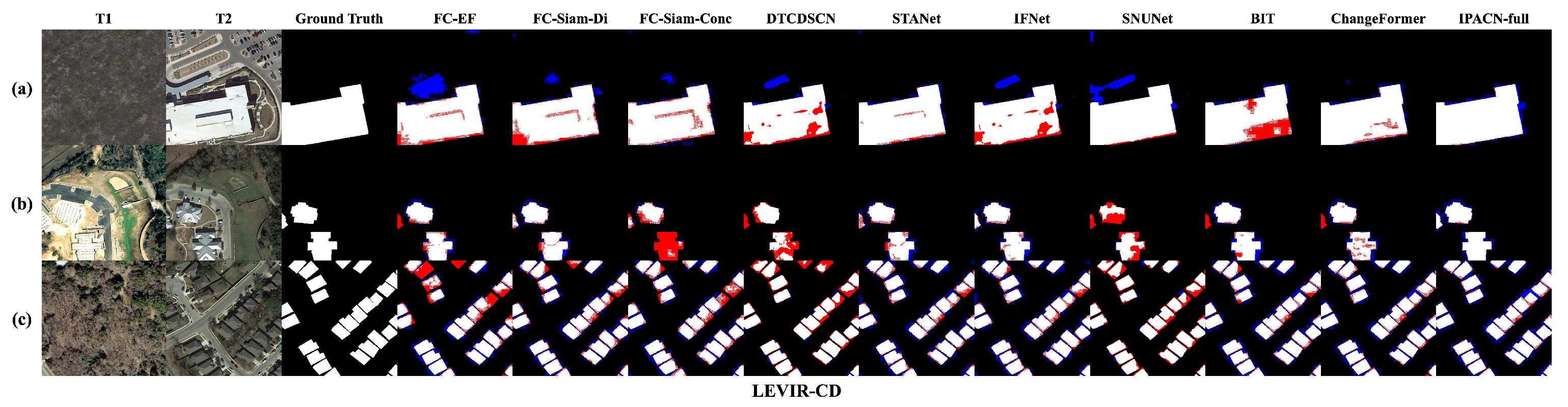
The LEVIR-CD dataset, characterized by diverse building changes, serves as a primary benchmark for evaluating our proposed IPACN. Visual comparisons of change detection maps from various methods are presented in Figure 6. These qualitative results illustrate the performance of IPACN (Full) in handling different scenarios. For instance, in rows (a) and (b), our model (last column) shows more precise boundary delineation for both large and small structures compared to methods like FC-Siam-Di [14] or STANet [29], which tend to produce more jagged edges or miss change areas. Row (c), which depicts a dense context with numerous newly constructed buildings, highlights IPACN’s proficiency. The model accurately identifies these small, scattered changes often missed by other approaches (e.g., FC-EF [14], BIT [16]), and demonstrates a significant reduction in both false negatives (missed changes, red) and false positives (false alarms, blue) when contrasted with models like SNUNet [15] and ChangeFormer [17].

Figure 6.
Qualitative comparison results on sample images from the LEVIR-CD test set. Methods shown (left to right after GT): FC-EF, FC-Siam-Di, FC-Siam-Conc, DTCDSCN, STANet, IFNet, SNUNet, BIT, ChangeFormer, IPACN (Full) (ours). Color coding: White = TP, black = TN, blue = FP, red = FN.The rows illustrate diverse building change scenarios: (a) detection of a large newly constructed building; (b) identification of a smaller-scale new structure; and (c) a challenging case with multiple small, densely-packed new buildings.
The quantitative performance of IPACN and other state-of-the-art methods on the LEVIR-CD test set is detailed in Table 2.
Table 2.
Quantitative comparison on the LEVIR-CD test set. Best results in bold.
In summary, on the LEVIR-CD dataset, IPACN demonstrates a strong capability to accurately detect building changes of varying scales and complexities. The qualitative results show improved boundary definition and fewer detection errors, while the quantitative metrics, particularly the F1 score and IoU, confirm its superior performance. This success is largely attributable to the IPB’s detail preservation and the FADEM’s adaptive enhancement, which work synergistically to overcome challenges posed by intricate urban environments and diverse change types, leading to high overall accuracy and balanced precision and recall.
4.4.2. Performance on WHU-CD Dataset
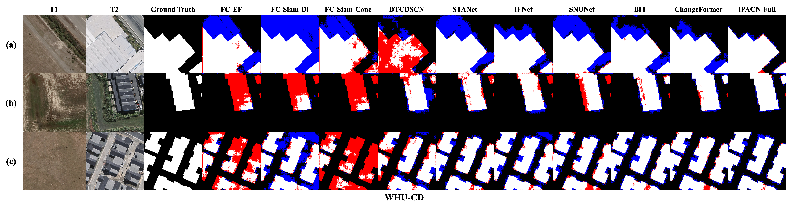
The WHU-CD dataset, comprising very high resolution (VHR) aerial images that primarily document building changes resulting from reconstruction activities, presents distinct challenges due to fine-grained object details and subtle contextual variations. The qualitative results on this dataset are depicted in Figure 7. These visualizations underscore IPACN (Full)’s proficiency in precisely localizing changes in VHR imagery. For instance, row (a) illustrates how IPACN generates significantly cleaner change maps with fewer false positives (blue areas) compared to methods such as DTCDSCN [36] and FC-Siam-Conc [14], which struggle with ambiguous non-change regions. In row (b), IPACN accurately identifies changes in closely situated buildings while effectively minimizing missed detections (red areas), a common issue for models like FC-Siam-Di [14] and STANet [29] in such scenarios. Furthermore, row (c) showcases IPACN’s ability to achieve more complete and accurate segmentation of complex change areas, contrasting with the fragmented or incomplete outputs from several other baseline methods.

Figure 7.
Qualitative comparison results on sample images from the WHU-CD test set. Methods shown (left to right after GT): FC-EF, FC-Siam-Di, FC-Siam-Conc, DTCDSCN, STANet, IFNet, SNUNet, BIT, ChangeFormer, IPACN (Full) (ours). Color coding: White = TP, black = TN, blue = FP, red = FN.The rows illustrate diverse change scenarios: (a) detection of a large newly constructed building; (b) identification of a smaller new structure; and (c) a challenging scenario involving multiple small, densely-packed new buildings.
Quantitative metrics for the WHU-CD dataset are presented in Table 3. IPACN (Full) once again demonstrates superior performance, achieving a leading F1 score of 94.52% and an IoU of 89.61%. These results significantly surpass those of the other evaluated methods, including the competitive ChangeFormer [17] (F1 = 89.05%, IoU = 80.26%). The IPACN-Base variant also exhibits strong performance, with an F1 score of 93.38% and an IoU of 87.59%, further validating the IPB’s capability to effectively process VHR data and preserve critical change information. The consistent high performance across the precision, recall, and overall accuracy metrics highlights the robustness of our full IPACN model in demanding VHR scenarios.
Table 3.
Quantitative comparison on the WHU-CD test set. Best results in bold.
In conclusion, for the WHU-CD dataset, IPACN’s architectural design, particularly the synergy between the Information-Preserving Backbone and the Frequency-Adaptive Difference Enhancement Module, proves highly effective. The model excels in accurately delineating building changes within VHR imagery characterized by post-reconstruction alterations. This is evident from its superior ability to capture fine details, minimize false alarms in spectrally similar non-changed areas, and maintain completeness in complex change regions, as reflected by its leading F1 score, IoU, and overall accuracy.
4.4.3. Performance on DSIFN-CD Dataset
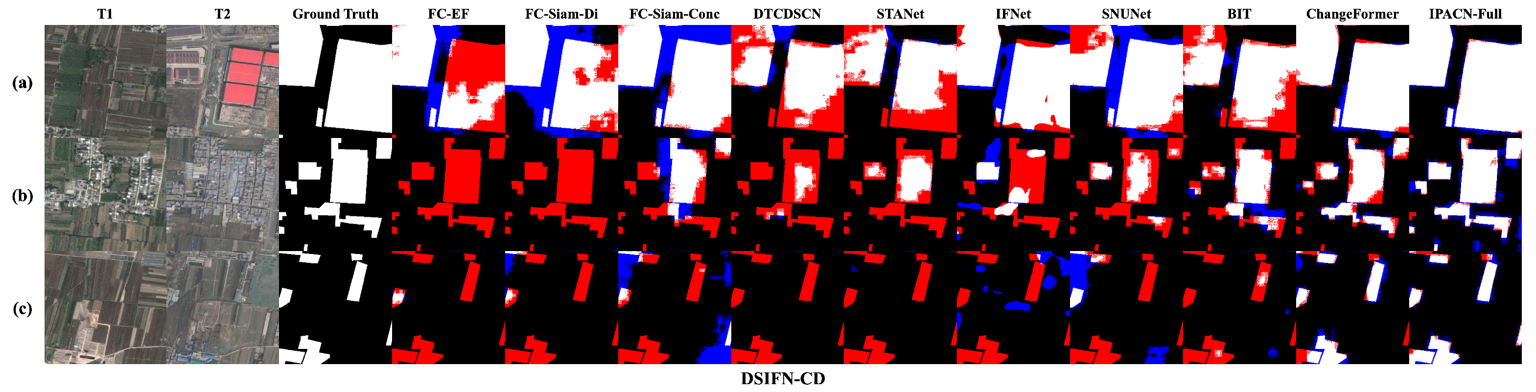
The DSIFN-CD dataset introduces a greater diversity of change scenarios, encompassing not only building alterations but also changes in various other land cover types such as agricultural land, bare soil, and road networks. Figure 8 provides qualitative comparisons on representative samples from this dataset. In row (a), which shows the large-scale conversion of agricultural land into prepared plots, IPACN (Full) achieves more complete detection with significantly fewer missed areas (false negatives, red) compared to baseline methods that struggle with these large, homogeneous change regions. Row (b) presents a complex mixed urban scene, where IPACN effectively identifies multiple scattered building changes with high accuracy and minimal fragmentation, outperforming approaches like FC-Siam-Di [14] and STANet [29] which produce noisy and incomplete results. Furthermore, row (c) illustrates another type of large-scale land-use change, where vegetated areas are converted into regular, rectangular plots. IPACN (Full) again demonstrates superior performance, precisely delineating the boundaries of these plots while other methods like IFNet [34] and BIT [16] either miss parts of the change or introduce significant false alarms.

Figure 8.
Qualitative comparison results on sample images from the DSIFN-CD test set. Methods shown (left to right after GT): FC-EF, FC-Siam-Di, FC-Siam-Conc, DTCDSCN, STANet, IFNet, SNUNet, BIT, ChangeFormer, IPACN (Full) (ours). Color coding: White = TP, black = TN, blue = FP, red = FN.The rows display different land cover change types: (a) large-scale conversion of agricultural land; (b) complex changes in a mixed urban scene; and (c) conversion of vegetation into regular rectangular plots.
The quantitative results on the DSIFN-CD dataset are summarized in Table 4. IPACN (Full) again achieves the leading performance, with an F1 score of 92.11% and an IoU of 85.18%. This demonstrates the model’s robustness and strong generalization across diverse change types beyond just building footprints. The IPACN-Base model also performs commendably (F1 = 90.75%, IoU = 83.05%), yet the notable improvement by the full IPACN model underscores the critical role of the FADEM in effectively handling heterogeneous changes by adaptively enhancing relevant difference features. The consistently high overall accuracy, along with balanced precision and recall, further reflects IPACN’s adaptability to varied land cover change scenarios.
Table 4.
Quantitative comparison on the DSIFN-CD test set. Best results in bold.
To summarize, the DSIFN-CD dataset, with its inclusion of diverse land cover changes, highlights the adaptability of IPACN. The model’s consistent top performance, evidenced by superior F1 score and IoU, demonstrates its capability to generalize beyond building-centric change detection. This success stems from the IPB’s robust feature preservation combined with the FADEM’s adaptive enhancement, which together allow IPACN to accurately identify a wider array of change types while maintaining precision and minimizing errors across heterogeneous scenes.
4.4.4. Performance on CDD Dataset
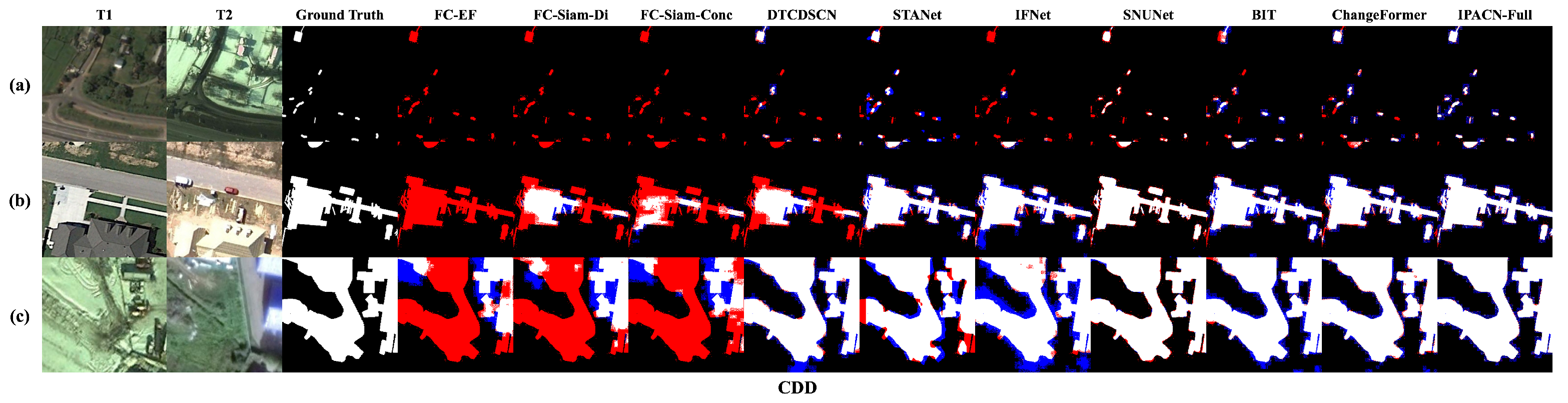
The Change Detection Dataset (CDD) is particularly challenging as it contains significant seasonal variations and illumination differences across bi-temporal images, demanding high robustness against pseudo-changes. Figure 9 visually demonstrates IPACN’s remarkable ability to overcome these challenges. The selected samples clearly exhibit strong pseudo-change signals, such as shifts in vegetation color (row a) and varying shadow conditions (row b). Despite these interferences, IPACN (Full) consistently produces exceptionally clean and accurate change maps, with minimal false positives (blue pixels). This contrasts sharply with methods like FC-Siam-Di [14] and STANet [29], which show a high number of errors under such conditions. Even advanced models like ChangeFormer [17] exhibit more false alarms in these illustrative examples when compared to our IPACN. Furthermore, row (c) highlights IPACN’s capability to precisely delineate complex change boundaries even amidst strong background variations.

Figure 9.
Qualitative comparison results on sample images from the CDD test set, showcasing robustness to seasonal and illumination variations. Methods shown (left to right after GT): FC-EF, FC-Siam-Di, FC-Siam-Conc, DTCDSCN, STANet, IFNet, SNUNet, BIT, ChangeFormer, IPACN (Full) (ours). Color coding: White = TP, black = TN, blue = FP, red = FN.The rows showcase the model’s robustness against challenging pseudo-changes: (a) a scene with significant seasonal variation; (b) a genuine change under strong illumination and shadow differences; and (c) a complex change object amidst severe background interference.
The quantitative evaluation on the CDD dataset, presented in Table 5, further substantiates these qualitative observations. IPACN (Full) achieves near-perfect scores across all reported metrics, with an F1 score of 99.27% and an IoU of 97.56%. These outstanding results significantly exceed all the other compared methods, underscoring the model’s exceptional robustness and its proficiency in accurately distinguishing genuine changes from seasonal and illumination-induced artifacts. IPACN-Base also performs impressively (F1 = 98.65%, IoU = 97.35%), but the further refinement by the FADEM in IPACN (Full) is crucial for achieving this level of near-perfect discrimination against pseudo-changes, as reflected in its superior precision, recall, and overall accuracy.
Table 5.
Quantitative comparison on the CDD test set. Best results in bold.
In essence, the results on the CDD dataset powerfully highlight IPACN’s primary strength: Its robustness against pseudo-changes stemming from seasonal and illumination variations. The FADEM component, in particular, demonstrates its effectiveness in adaptively filtering out these interferences while preserving true change information identified by the IPB. This capability is critical for reliable change detection in real-world applications, where such variations are common, leading to the exceptionally high F1 score, IoU, and overall accuracy achieved by our model.
4.5. Ablation Studies
To validate the effectiveness and quantify the contribution of the core components within our proposed IPACN framework—namely, the Information-Preserving Backbone (IPB) and the Frequency-Adaptive Difference Enhancement Module (FADEM)—we conducted a series of ablation studies. These experiments were performed on the challenging LEVIR-CD dataset. It is important to note that for this specific analysis we utilized a different model configuration than in the main comparative experiments. While the main results (Table 2, Table 3, Table 4 and Table 5) were generated using the standard IPACN-Base setup (e.g., , channels = [72, …]), the ablation studies were conducted with a ’large’ configuration (, channels = [128, 256, 512, 1024]). This choice was made to rigorously test the impact of our core components in a high-capacity setting, where their architectural benefits could be isolated more distinctly. We compare our full IPACN model against several configurations derived from it: (1) IPACN with a non-reversible version of our IPB (termed “IPACN (IPB Non-Rev.)”), where standard forward/backward propagation replaces the reversible mechanism; (2) IPACN with the reversible IPB but without the FADEM (termed “IPACN (IPB Rev.)”). All IPACN variants in the ablation study utilize the ‘large’-scale backbone configuration (channels = [128, 256, 512, 1024], layers = [1, 2, 6, 2], ), as detailed in Section 4.2.1. The performance metrics (in %) are summarized in Table 6, and the corresponding model complexities for the IPACN variants are reported in Table 7. Note that the BIT baseline [16] mentioned in previous comparisons serves as an external reference point but is not included in the direct IPACN component ablation complexity analysis.
Table 6.
Ablation study performance metrics on the LEVIR-CD test set (units in %). “IPB Rev.” indicates reversible connections. “FADEM” indicates the enhancement module. Best results in bold. Baseline BIT is included for performance context.
Table 7.
Model complexity comparison for IPACN variants in the ablation study.
4.5.1. Impact of the Information-Preserving Backbone (IPB) Structure and Reversible Connections
The IPB forms the core of our feature extraction strategy. Comparing the non-reversible IPB against the external BIT baseline (Table 6) shows the inherent advantage of the IPB’s multi-column structure (F1: 90.00% vs. 89.31%).
The primary advantage of incorporating reversible connections becomes evident when comparing “IPACN (IPB Rev.)” with “IPACN (IPB Non-Rev.)”. The reversible version achieves superior performance (Table 6: F1+1.30%, IoU+2.18%). Crucially, this improvement is achieved while leveraging the primary benefit of reversible architectures–substantially reduced GPU memory consumption during training. As established in [20], reversible connections allow activations to be recomputed on the fly during the backward pass instead of being stored, theoretically offering memory overhead with increasing depth or column numbers. This efficiency is particularly vital for VHR remote sensing CD. It means that **within the same GPU memory constraints, one could train a considerably deeper or wider IPACN model using the reversible IPB compared to a non-reversible equivalent, potentially unlocking further performance gains with different, larger parameter configurations**. Thus, the reversible IPB not only enhances performance through better information preservation (leading to more discriminative features for accurate change identification) but also offers crucial scalability by enabling the training of more powerful models on memory-limited hardware, essential for handling large VHR datasets. While the inference complexities (params/FLOPs; see Table 7) remain similar between the reversible and non-reversible IPB variants (273 M Params, 39.0 G FLOPs), the training memory efficiency represents a major practical advantage of adopting the reversible principle in the IPB, facilitating better model scaling and handling of high-resolution data. The performance gains themselves further underscore that minimizing information loss through reversibility leads to more discriminative features, essential for accurate change detection.
4.5.2. Contribution of the Frequency-Adaptive Difference Enhancement Module (FADEM)
Adding the FADEM to the reversible IPB yields the full “IPACN (Full)” model, achieving the best overall performance (Table 6; F1: 92.49%, IoU: 85.05%). Compared to the IPB Rev. version, the FADEM provides a significant boost (F1+1.19%, IoU+1.07%), while significantly increasing model complexity (Table 7). This substantial gain highlights the FADEM’s effectiveness in adaptively refining the bi-temporal difference features. By dynamically adjusting its spatial context aggregation and filtering based on local frequency characteristics (Section 3.4), the FADEM enhances salient change signals and suppresses noise/pseudo-changes, prevalent in VHR imagery, leading to more precise and robust detection.
4.5.3. Overall Performance and Synergy
The ablation results (Table 6) show a clear benefit from each component of IPACN. The IPB structure provides a strong foundation. Its reversible nature enhances feature quality via information preservation and critically enables **training larger, potentially more performant models under fixed memory budgets** due to its efficiency. The FADEM then provides substantial refinement by adaptively processing difference features. The top performance of the full IPACN model (F1: 92.49%, IoU: 85.05%) demonstrates the powerful synergy between efficient, high-fidelity feature extraction and adaptive difference enhancement, validating our design choices for VHR change detection. These ablation studies robustly validate our design choices, highlighting the individual and combined contributions of information preservation (with associated training efficiency) and frequency-adaptive enhancement to achieving state-of-the-art change detection accuracy on the LEVIR-CD dataset.
4.6. Analysis of Information Preservation and Frequency Adaptation Benefits
While the quantitative results and ablation studies confirm the overall effectiveness of IPACN and its components, this section provides a deeper, qualitative analysis of the underlying mechanisms contributing to its performance, focusing on the benefits derived from the principles of information preservation and frequency adaptation.
5. Discussion
The comprehensive experimental results presented in Section 4, particularly the ablation studies summarized in Table 6, strongly validate the effectiveness of the proposed Information-Preserving Adaptive Convolutional Network (IPACN) for VHR remote sensing change detection. IPACN consistently achieved state-of-the-art performance across multiple benchmark datasets, demonstrating significant improvements over existing CNN, attention-based, and Transformer methodologies. This section delves deeper into the underlying reasons for IPACN’s success by discussing the distinct advantages conferred by its core components—the Information-Preserving Backbone (IPB) and the Frequency-Adaptive Difference Enhancement Module (FADEM)—and their synergistic interplay.
5.1. Benefits of Information Preservation via Reversible IPB
A key factor contributing to IPACN’s performance is the IPB’s ability to mitigate information loss during hierarchical feature extraction. Inspired by reversible network principles [7,20], the IPB employs multi-column processing with reversible inter-column connections. As evidenced by the ablation study (Table 6), enabling reversible connections (“IPACN (IPB Rev.)”) yields a notable improvement in F1 score (+1.30%) and IoU (+2.18%) compared to the identical architecture with standard, non-reversible backpropagation (“IPACN (IPB Non-Rev.)”), despite having the same parameter count and FLOPs. This confirms that the quasi-lossless information propagation inherent in the reversible design is beneficial for CD. By preserving fine-grained spatial details—crucial for identifying subtle changes, delineating complex boundaries, and detecting small objects, often lost in conventional downsampling—the IPB provides a higher-fidelity feature foundation for subsequent analysis. Furthermore, this reversible architecture offers significant potential for training efficiency, drastically reducing GPU memory consumption by reconstructing activations during backpropagation [20], which is invaluable for handling large VHR images or scaling to larger models.
5.2. Advantages of Frequency-Adaptive Difference Enhancement (FADEM)
While the IPB ensures high-quality feature extraction, the FADEM module plays a crucial role in refining the crucial bi-temporal difference features (). Difference maps in remote sensing are often noisy and contain a mix of true change signals, pseudo-changes, and background clutter, exhibiting significant spatial heterogeneity in their frequency content. The FADEM addresses this by adapting concepts from frequency-aware processing [12]. As shown in Table 7, incorporating the FADEM (“IPACN (Full)”) provides a substantial performance boost over the IPB alone (“IPACN (IPB Rev.)”), improving the F1 score by 1.19% and IoU by 1.07% on LEVIR-CD. This demonstrates the FADEM’s effectiveness. By dynamically adjusting its spatial context aggregation (akin to adaptive dilation) and filtering frequency response based on the local spectral characteristics of the difference map, the FADEM can intelligently enhance salient change features (e.g., high frequencies at boundaries) while suppressing irrelevant variations (e.g., low-frequency illumination shifts or high-frequency noise). This adaptive contextualization and filtering leads to cleaner, more discriminative change representations and contributes to the model’s improved robustness against pseudo-changes, a common challenge in real-world CD scenarios.
5.3. Synergy Between Information Preservation and Adaptation
The superior performance of the full IPACN framework stems significantly from the synergy between the IPB and FADEM. The IPB provides the high-fidelity, detail-rich features necessary for accurate analysis. The FADEM then leverages this high-quality input, applying its frequency-adaptive capabilities to selectively enhance the true change signals embedded within the difference features, while mitigating noise and adapting to the diverse spectral nature of changes and non-changes. This sequential process—preserving details first with the IPB, then adaptively refining the relevant differences with the FADEM—allows IPACN to outperform methods that may suffer from either initial information loss or subsequent non-adaptive processing of potentially degraded difference features.
5.4. Computational Complexity Considerations
A comprehensive assessment of the IPACN framework necessitates a discussion of its computational profile. The design of the Information-Preserving Backbone (IPB), with its multi-column architecture inspired by reversible networks, is intentionally high-capacity. This choice was made to rigorously test the upper limits of performance by minimizing information loss, a primary bottleneck in VHR change detection. Consequently, our IPACN models, particularly the full version, inherently demand a greater computational budget in terms of parameter count and FLOPs compared to standard single-stream CNNs or some more streamlined Transformer architectures. We acknowledge this as a significant trade-off between performance and efficiency. Our current study focuses on achieving state-of-the-art accuracy; however, as we have noted in our limitations, this higher complexity may pose challenges for applications on resource-constrained platforms. Therefore, a critical direction for future work, as outlined in the subsequent discussion on limitations, is the development of lightweight IPACN variants through model compression and optimization techniques.
5.5. Potential for Long-Term Time-Series Analysis and Large-Scale Generalization
A critical aspect for any change detection model is its potential to scale from bi-temporal analysis of curated patches to robust, large-scale, and long-term monitoring. This extension presents significant challenges, including the accumulation of pseudo-changes over time and the need to preserve fine-grained details for tracking subtle dynamics, an issue of importance in applications such as annual land cover mapping [37]. While IPACN is architected for bi-temporal inputs, its design principles offer a strong foundation for these advanced scenarios. For long-term analysis, a straightforward approach is to apply the model sequentially to pairwise images (e.g., year-to-year) to derive a series of change maps.
The inherent architecture of IPACN is particularly suited to overcome the challenges of this scaled-up application. The primary obstacle in long-term and large-area analysis is the compounding effect of pseudo-changes from inconsistent acquisition conditions. Our Frequency-Adaptive Difference Enhancement Module (FADEM) is intrinsically designed to tackle this. Rather than relying on static filters that may fail on unseen variations, the FADEM’s frequency-adaptive mechanism dynamically adjusts its response to local signal characteristics. This provides the inherent robustness needed to suppress diverse, acquisition-related noise signatures and maintain high fidelity across large datasets with significant temporal and spatial variance. Concurrently, meaningful long-term monitoring requires the preservation of fine-grained details to accurately track subtle or incremental changes. The information-preserving design of ourInformation-Preserving Backbone (IPB) is fundamental to this goal. By minimizing feature degradation, the IPB ensures that the essential spatial details required to identify small or complex changes are not lost, which is vital for accurate historical analysis. In summary, the synergy of the IPB’s detail preservation and the FADEM’s adaptive robustness provides a strong theoretical basis for IPACN’s applicability to large-scale, long-term monitoring. Future work should focus on empirically validating this potential and exploring optimizations for efficient large-area processing.
5.6. Limitations and Future Directions
Despite its demonstrated strengths, IPACN has limitations that present avenues for future work. The primary limitation is the computational complexity of the full model. As shown in Table 7, the multi-column backbone results in a high parameter count and significant FLOPs, which could hinder deployment on resource-constrained platforms. Future research should focus on developing lightweight IPACN variants. Several strategies could be pursued. (1) Structured pruning: The parallel-column architecture of the IPB may contain redundancies, making it a strong candidate for structured pruning to remove less salient columns or channels, thereby creating a more efficient backbone. (2) Quantization: Converting the model’s weights from 32-bit floating-point precision to lower-bit representations (e.g., INT8) would substantially reduce the memory footprint and accelerate inference on compatible hardware. (3) Knowledge distillation: This is a particularly compelling approach, where the high-performance IPACN could serve as a ‘teacher’ model to guide the training of a smaller ‘student’ network, enabling the student to learn the teacher’s capabilities while maintaining a much lower computational budget.
Furthermore, IPACN currently relies on supervised learning. Exploring self-supervised or semi-supervised pre-training strategies tailored for this architecture could significantly reduce the dependence on extensive pixel-level annotations, broadening its practical applicability. Extending the framework to multi-class change detection or adapting it for diverse sensor modalities (e.g., SAR) represent other valuable avenues for future research.
6. Conclusions
Remote sensing change detection using very high resolution (VHR) imagery is essential for monitoring dynamic environmental and anthropogenic processes, but faces challenges from complex scenes, subtle changes, pseudo-change artifacts, and information loss in conventional deep learning models. This paper introduced Information-Preserving Adaptive Convolutional Network (IPACN), a novel framework designed to overcome these limitations.
IPACN uniquely integrates two core concepts: an Information-Preserving Backbone, inspired by reversible network principles, which minimizes feature degradation during hierarchical extraction; and a Frequency-Adaptive Difference Enhancement Module (FADEM), which adapts frequency-aware processing techniques to intelligently refine bi-temporal difference features based on their local frequency content. This synergistic combination aims to produce change representations that are both rich in detail and robust to noise and irrelevant variations.
Extensive experiments on four standard benchmark datasets demonstrated that IPACN achieves state-of-the-art performance, surpassing various CNN, attention-based, and Transformer-based methods in F1 score and IoU. Ablation studies and specific analyses confirmed the significant contributions of both the information-preserving architecture and the frequency-adaptive enhancement strategy. The results highlight IPACN’s improved capability for accurate boundary delineation, detection of small changes, and enhanced robustness, particularly in challenging VHR scenarios.
By pioneering the integration of information preservation and frequency-adaptive processing specifically tailored for change detection, IPACN presents a powerful and effective new direction for analyzing Earth’s surface dynamics from remote sensing data. Future work will focus on improving computational efficiency, reducing label dependency, and extending the framework’s applicability.
Author Contributions
Conceptualization, H.Q., J.L. and X.G.; methodology, H.Q. and F.W.; software, H.Q. and X.G.; validation, J.L., F.W. and X.G.; formal analysis, X.G.; investigation, X.G. and J.L.; resources, H.Q.; data curation, H.Q.; writing—original draft, H.Q. and X.G.; writing—review and editing, J.L.; visualization, F.W.; supervision, X.G.; project administration, X.G.; funding acquisition, X.G. All authors have read and agreed to the published version of the manuscript.
Funding
This work was supported by the Xinjiang Tianshan Talent Program (No. 2022TSYCLJ0002), the Basic Frontier Project of the Xinjiang Institute of Ecology and Geography, Chinese Academy of Sciences (No. E3500201), and the Youth Interdisciplinary Innovation Team of the Key State Laboratory of Ecological Safety and Sustainable Development in Arid Lands (No. E4500125).
Data Availability Statement
The datasets analyzed during the current study are publicly available and are cited accordingly in the manuscript.
Conflicts of Interest
The authors declare no conflicts of interest.
References
- Jiang, W.; Sun, Y.; Lei, L.; Kuang, G.; Ji, K. Change detection of multisource remote sensing images: A review. Int. J. Digit. Earth 2024, 17, 2398051. [Google Scholar] [CrossRef]
- Cheng, G.; Huang, Y.; Li, X.; Lyu, S.; Xu, Z.; Zhao, H.; Zhao, Q.; Xiang, S. Change detection methods for remote sensing in the last decade: A comprehensive review. Remote Sens. 2024, 16, 2355. [Google Scholar] [CrossRef]
- Hussain, M.; Chen, D.; Cheng, A.; Wei, H.; Stanley, D. Change detection from remotely sensed images: From pixel-based to object-based approaches. ISPRS J. Photogramm. Remote Sens. 2013, 80, 91–106. [Google Scholar] [CrossRef]
- Wu, C.; Du, B.; Zhang, L. Fully convolutional change detection framework with generative adversarial network for unsupervised, weakly supervised and regional supervised change detection. IEEE Trans. Pattern Anal. Mach. Intell. 2023, 45, 9774–9788. [Google Scholar] [CrossRef]
- Khelifi, L.; Mignotte, M. Deep learning for change detection in remote sensing images: Comprehensive review and meta-analysis. IEEE Access 2020, 8, 126385–126400. [Google Scholar] [CrossRef]
- Shafique, A.; Cao, G.; Khan, Z.; Asad, M.; Aslam, M. Deep learning-based change detection in remote sensing images: A review. Remote Sens. 2022, 14, 871. [Google Scholar] [CrossRef]
- Cai, Y.; Zhou, Y.; Han, Q.; Sun, J.; Kong, X.; Li, J.; Zhang, X. Reversible column networks. arXiv 2022, arXiv:2212.11696. [Google Scholar]
- Peng, D.; Zhang, Y.; Guan, H. End-to-end change detection for high resolution satellite images using improved UNet++. Remote Sens. 2019, 11, 1382. [Google Scholar] [CrossRef]
- Zheng, Z.; Wan, Y.; Zhang, Y.; Xiang, S.; Peng, D.; Zhang, B. CLNet: Cross-layer convolutional neural network for change detection in optical remote sensing imagery. ISPRS J. Photogramm. Remote Sens. 2021, 175, 247–267. [Google Scholar] [CrossRef]
- Hu, C.; Ma, M.; Ma, X.; Zhang, H.; Wu, D.; Gao, G.; Zhang, W. STANet: Spatiotemporal Adaptive Network for Remote Sensing Images. In Proceedings of the 2023 IEEE International Conference on Image Processing (ICIP), Kuala Lumpur, Malaysia, 8–11 October 2023; pp. 3429–3433. [Google Scholar]
- Zhang, J.; Shao, Z.; Ding, Q.; Huang, X.; Wang, Y.; Zhou, X.; Li, D. AERNet: An attention-guided edge refinement network and a dataset for remote sensing building change detection. IEEE Trans. Geosci. Remote Sens. 2023, 61, 1–16. [Google Scholar] [CrossRef]
- Chen, L.; Gu, L.; Zheng, D.; Fu, Y. Frequency-adaptive dilated convolution for semantic segmentation. In Proceedings of the IEEE/CVF Conference on Computer Vision and Pattern Recognition, Seattle, WA, USA, 17–18 June 2024; pp. 3414–3425. [Google Scholar]
- Peng, X.; Zhong, R.; Li, Z.; Li, Q. Optical remote sensing image change detection based on attention mechanism and image difference. IEEE Trans. Geosci. Remote Sens. 2020, 59, 7296–7307. [Google Scholar] [CrossRef]
- Daudt, R.C.; Le Saux, B.; Boulch, A. Fully convolutional siamese networks for change detection. In Proceedings of the 2018 25th IEEE international conference on image processing (ICIP), Athens, Greece, 7–10 October 2018; pp. 4063–4067. [Google Scholar]
- Fang, S.; Li, K.; Shao, J.; Li, Z. SNUNet-CD: A densely connected Siamese network for change detection of VHR images. IEEE Geosci. Remote Sens. Lett. 2021, 19, 1–5. [Google Scholar] [CrossRef]
- Chen, H.; Qi, Z.; Shi, Z. Remote sensing image change detection with transformers. IEEE Trans. Geosci. Remote Sens. 2021, 60, 1–14. [Google Scholar] [CrossRef]
- Bandara, W.G.C.; Patel, V.M. A transformer-based siamese network for change detection. In Proceedings of the IGARSS 2022—2022 IEEE International Geoscience and Remote Sensing Symposium, Kuala Lumpur, Malaysia, 7–22 July 2022; pp. 207–210. [Google Scholar]
- Tishby, N.; Pereira, F.C.; Bialek, W. The information bottleneck method. arXiv 2000, arXiv:physics/0004057. [Google Scholar]
- Liu, Z.; Mao, H.; Wu, C.Y.; Feichtenhofer, C.; Darrell, T.; Xie, S. A convnet for the 2020s. In Proceedings of the IEEE/CVF Conference on Computer Vision and Pattern Recognition, New Orleans, LA, USA, 19–20 June 2022; pp. 11976–11986. [Google Scholar]
- Gomez, A.N.; Ren, M.; Urtasun, R.; Grosse, R.B. The reversible residual network: Backpropagation without storing activations. In Advances in Neural Information Processing Systems; Curran Associates, Inc.: Red Hook, NY, USA, 2017; Volume 30. [Google Scholar]
- Vaswani, A.; Shazeer, N.; Parmar, N.; Uszkoreit, J.; Jones, L.; Gomez, A.N.; Kaiser, Ł.; Polosukhin, I. Attention is all you need. In Advances in Neural Information Processing Systems; Curran Associates, Inc.: Red Hook, NY, USA, 2017; Volume 30. [Google Scholar]
- Zhao, J.; Jiao, L.; Wang, C.; Liu, X.; Liu, F.; Li, L.; Yang, S. GeoFormer: A geometric representation transformer for change detection. IEEE Trans. Geosci. Remote Sens. 2023, 61, 1–17. [Google Scholar] [CrossRef]
- Ronneberger, O.; Fischer, P.; Brox, T. U-net: Convolutional networks for biomedical image segmentation. In Proceedings of the Medical Image Computing and Computer-Assisted Intervention–MICCAI 2015: 18th International Conference, Munich, Germany, 5–9 October 2015; Proceedings, Part III 18. Springer: Berlin/Heidelberg, Germany, 2015; pp. 234–241. [Google Scholar]
- Soydaner, D. Attention mechanism in neural networks: Where it comes and where it goes. Neural Comput. Appl. 2022, 34, 13371–13385. [Google Scholar] [CrossRef]
- Mangalam, K.; Fan, H.; Li, Y.; Wu, C.Y.; Xiong, B.; Feichtenhofer, C.; Malik, J. Reversible vision transformers. In Proceedings of the IEEE/CVF Conference on Computer Vision and Pattern Recognition, New Orleans, LA, USA, 19–20 June 2022; pp. 10830–10840. [Google Scholar]
- Zhu, X.; Hu, H.; Lin, S.; Dai, J. Deformable convnets v2: More deformable, better results. In Proceedings of the IEEE/CVF Conference on Computer Vision and Pattern Recognition (CVPR), Long Beach, CA, USA, 5–20 June 2019; pp. 9308–9316. [Google Scholar]
- Jia, X.; De Brabandere, B.; Tuytelaars, T.; Gool, L.V. Dynamic filter networks. In Advances in Neural Information Processing Systems; Curran Associates, Inc.: Red Hook, NY, USA, 2016; Volume 29. [Google Scholar]
- Chen, L.C.; Zhu, Y.; Papandreou, G.; Schroff, F.; Adam, H. Encoder-decoder with atrous separable convolution for semantic image segmentation. In Proceedings of the European Conference on Computer Vision (ECCV), Munich, Germany, 8–14 September 2018; pp. 801–818. [Google Scholar]
- Chen, H.; Shi, Z. A spatial-temporal attention-based method and a new dataset for remote sensing image change detection. Remote Sens. 2020, 12, 1662. [Google Scholar] [CrossRef]
- Shi, Q.; Liu, M.; Li, S.; Liu, X.; Wang, F.; Zhang, L. A deeply supervised attention metric-based network and an open aerial image dataset for remote sensing change detection. IEEE Trans. Geosci. Remote Sens. 2021, 60, 1–16. [Google Scholar] [CrossRef]
- Chen, L.C.; Papandreou, G.; Schroff, F.; Adam, H. Rethinking atrous convolution for semantic image segmentation. arXiv 2017, arXiv:1706.05587. [Google Scholar]
- Ji, S.; Wei, S.; Lu, M. Fully convolutional networks for multisource building extraction from an open aerial and satellite imagery data set. IEEE Trans. Geosci. Remote Sens. 2018, 57, 574–586. [Google Scholar] [CrossRef]
- Lebedev, M.; Vizilter, Y.V.; Vygolov, O.; Knyaz, V.A.; Rubis, A.Y. Change detection in remote sensing images using conditional adversarial networks. Int. Arch. Photogramm. Remote Sens. Spat. Inf. Sci. 2018, 42, 565–571. [Google Scholar] [CrossRef]
- Zhang, C.; Yue, P.; Tapete, D.; Jiang, L.; Shangguan, B.; Huang, L.; Liu, G. A deeply supervised image fusion network for change detection in high resolution bi-temporal remote sensing images. ISPRS J. Photogramm. Remote Sens. 2020, 166, 183–200. [Google Scholar] [CrossRef]
- Loshchilov, I.; Hutter, F. Decoupled weight decay regularization. arXiv 2017, arXiv:1711.05101. [Google Scholar]
- Liu, Y.; Pang, C.; Zhan, Z.; Zhang, X.; Yang, X. Building change detection for remote sensing images using a dual-task constrained deep siamese convolutional network model. IEEE Geosci. Remote Sens. Lett. 2020, 18, 811–815. [Google Scholar] [CrossRef]
- He, D.; Shi, Q.; Liu, X.; Zhong, Y.; Xia, G.; Zhang, L. Generating annual high resolution land cover products for 28 metropolises in China based on a deep super-resolution mapping network using Landsat imagery. GIScience Remote Sens. 2022, 59, 2036–2067. [Google Scholar] [CrossRef]
Disclaimer/Publisher’s Note: The statements, opinions and data contained in all publications are solely those of the individual author(s) and contributor(s) and not of MDPI and/or the editor(s). MDPI and/or the editor(s) disclaim responsibility for any injury to people or property resulting from any ideas, methods, instructions or products referred to in the content. |
© 2025 by the authors. Licensee MDPI, Basel, Switzerland. This article is an open access article distributed under the terms and conditions of the Creative Commons Attribution (CC BY) license (https://creativecommons.org/licenses/by/4.0/).