Abstract
The interaction between atmospheric moisture condensation (AMC) on leaf surfaces and vegetation health is an emerging area of research, particularly relevant for advancing our understanding of water–vegetation dynamics in the contexts of remote sensing and hydrology. AMC, particularly in the form of dew, plays a vital role in both hydrological and ecological processes. The presence of AMC on leaf surfaces serves as an indicator of leaf water potential and overall ecosystem health. However, the large-scale assessment of AMC on leaf surfaces remains limited. To address this gap, we propose a leaf area index (LAI)-derived condensation potential (LCP) index to estimate potential dew yield, thereby supporting more effective land management and resource allocation. Based on psychrometric principles, we apply the nocturnal condensation potential index (NCPI), using dew point depression (ΔT = Ta − Td) and vapor pressure deficit derived from field meteorological data. Kriging interpolation is used to estimate the spatial and temporal variations in the AMC. For management applications, we develop a management suitability score (MSS) and prioritization (MSP) framework by integrating the NCPI and the LAI. The MSS values are classified into four MSP levels—High, Moderate–High, Moderate, and Low—using the Jenks natural breaks method, with thresholds of 0.15, 0.27, and 0.37. This classification reveals cases where favorable weather conditions coincide with low ecological potential (i.e., low MSS but high MSP), indicating areas that may require active management. Additionally, a pairwise correlation analysis shows that the MSS varies significantly across different LULC types but remains relatively stable across groundwater potential zones. This suggests that the MSS is more responsive to the vegetation and micrometeorological variability inherent in LULC, underscoring its unique value for informed land use management. Overall, this study demonstrates the added value of the LAI-derived AMC modeling for monitoring spatiotemporal micrometeorological and vegetation dynamics. The MSS and MSP framework provides a scalable, data-driven approach to adaptive land use prioritization, offering valuable insights into forest health improvement and ecological water management in the face of climate change.
1. Introduction
Climate policies aimed at achieving net-zero emissions highlight the importance of natural-based solutions, especially carbon sinks such as forests. The land-use, land-use change, and forestry (LULUCF) sector has become pivotal in reducing atmospheric carbon dioxide levels, as vegetation plays a significant role in carbon sequestration [1]. Healthy vegetation, however, depends on adequate water availability, making ecological water requirements essential for sustaining various land uses and land covers (LULC). Understanding vegetation–water dynamics is essential as climate change intensifies water stress, particularly in the agricultural and forest ecosystems [2,3].
The leaf area index (LAI) is defined as the total one-sided leaf surface area per unit ground surface area (m2/m2). It is a fundamental biophysical parameter used to characterize vegetation structure, to quantify canopy density, and to assess photosynthetic capacity [4]. The LAI is essential for evaluating dynamic land-use changes, particularly in managed ecosystems such as agroforests. Long-term in situ monitoring further underscores its critical role in energy exchange, climate response, and vegetation adaptation to environmental change [5]. This significance is supported by remote sensing applications, including airborne laser scanning and satellite-based observations [6]. Recent advances highlight the potential of LiDAR-derived metrics to capture vertical canopy structure and to enhance the forest LAI estimation accuracy across diverse forest types [7]. Furthermore, to mitigate saturation effects commonly observed in traditional vegetation indices under dense canopy conditions, improved methods such as the use of a negative soil adjustment factor in the soil-adjusted vegetation index have shown promise in refining the LAI estimates in high-density vegetative areas [8]. Linking hydrologically weighted LAI with local precipitation provides insights into the vegetation’s influence on hydrological cycles, demonstrating that global vegetation changes can enhance water availability and can help mitigate global water decline [9]. Leaf water potential (LWP) is a key indicator of plant water status, reflecting how plants respond to water stress and employ mechanisms to avoid dehydration [10]. In response to drought stress and limited water availability, plants activate various coping mechanisms, including a reduction in the LWP [11]. This is often accompanied by a decrease in turgor pressure, stomatal closure, and reduced cell growth, all of which contribute to conserving water [12]. Remote sensing and satellite-based indices, such as temperature–soil moisture dryness indices, have proven effective in monitoring agricultural drought stress and water availability [13,14].
In addition to soil moisture, atmospheric moisture can act as a supplemental water source, particularly in arid and semi-arid environments. Dew, a prevalent form of atmospheric moisture condensation (AMC), can be absorbed by plants through foliar uptake, directly increasing the LWP and aiding plant survival in water-limited environments [15]. Dew not only supplies moisture but affects the energy balance of vegetation by lowering leaf temperatures through evaporative cooling, modifying surface albedo, and altering emissivity [16,17]. In agricultural environments, dew presents both advantages and drawbacks; it supports plant growth in regions with limited rainfall [18,19], but it can also promote fungal development and plant pathogens, potentially leading to crop diseases [20,21,22]. Although dew contributes only a small fraction to the Earth’s total water budget, it plays a vital role in local hydrological processes, and helps maintain ecosystem stability. Dew formation varies across different surfaces, including polyethylene foils, grass, soil, leaves, and sand particles [23,24,25,26,27], and is influenced by factors like humidity, temperature differentials, wind speed, and clear skies [19,28]. Studies employing dew formation models [29,30,31,32,33] and kriging interpolation methods [34,35] have produced valuable insights into regional dew patterns, deepening our understanding of micrometeorological processes and informing water management strategies in arid regions.
In ecosystems defined by precipitation, such as deserts, grasslands, and forests, dew serves as an important moisture source during dry periods, thereby contributing to overall ecosystem stability. For instance, in China’s Gurbantünggüt Desert, dew forms frequently but in small amounts, with an average annual accumulation of approximately 12.21 mm. It contributes around 9% to the regional water balance, particularly during spring and autumn when humidity levels favor dew formation [36]. In a continental semiarid grassland, dew was observed on 39% of the nights, with each event lasting an average of 5 ± 4 h. The average daily dew deposition was 0.2 mm, with peak values reaching up to 0.7 mm. Annual dew accumulation ranged from 16.5 to 69 mm, accounting for 4.9% to 10.2% of the total annual precipitation. During the dry season, dew contributed up to 33.6% of the seasonal rainfall, helping to alleviate local water shortages [37]. In the eastern Amazon rainforest, dew significantly enhances canopy moisture, especially during the dry season. Dew events last an average of 10.4 h and, under dry conditions, can contribute up to 50% of the ambient humidity [38]. Together, these findings underscore the ecosystem-specific and seasonal significance of dew, highlighting its role not only in plant water relations but in broader hydrological and energy dynamics.
The interaction between the AMC on leaves and vegetation health is an emerging area of interest, particularly within the fields of remote sensing and hydrology [39,40,41]. Estimating the water on leaf surfaces through energy balance models [17,42,43] and remote sensing technologies [44,45], such as radar backscatter and brightness temperature measurements, provides valuable insights into the dynamics of water–vegetation interactions. Although dew typically accumulates in small amounts—around 0.4 mm per event—previous studies have shown that it plays a crucial role in maintaining canopy moisture, especially during dry periods [22]. These advancements significantly improve our capacity to monitor vegetation health and hydrological processes across multiple spatial and temporal scales. The research has highlighted the significant influence of vegetation–groundwater interactions in shaping the LULC distribution, diversity, and structure, especially in groundwater-dependent ecosystems [46,47], underscoring the need for regional-scale estimation methods. The integration of remote sensing (RS) and geographic information systems (GIS) has proven to be an effective tool for conducting such assessments [48,49]. Assessing the groundwater potential (GWP) requires a comprehensive analysis of multiple factors, including geology, topography, drainage patterns, and remote sensing-derived indices, such as the normalized difference vegetation index (NDVI), soil moisture index, and lineament extraction [50,51].
The existing dew estimation methods vary in their complexity, data requirements, and spatial applicability. Energy balance models offer physically robust estimates of dew formation; however, their reliance on detailed input parameters—such as net radiation, wind speed, and surface emissivity—limits their scalability in data-scarce regions. Empirical models often depend on site-specific coefficients and require additional inputs, such as cloud cover, which can limit their generalizability. Remote sensing approaches utilizing radar backscatter and brightness temperature enable large-scale monitoring; however, they are prone to errors caused by vegetation structure, surface roughness, and atmospheric interference, and often require frequent calibration to maintain accuracy.
By contrast, this study presents a simplified and scalable framework for estimating condensation potential, grounded in psychrometric principles and relying solely on field-measured temperature, relative humidity, and dew point. This approach reduces data dependency, making it particularly well-suited for regions with limited monitoring infrastructure. Furthermore, by integrating the LAI and the AMC, the proposed framework quantifies their combined influence on the LULC dynamics. This practical method enhances regional-scale assessments and supports data-driven land management by emphasizing the hydrological contributions of vegetation and atmospheric moisture under changing environmental conditions.
2. Materials and Methods
2.1. Study Area
In alignment with the growing emphasis on forest management and catchment-scale meteorological analysis [5,9,52], the study area was located in the central catchments of Taiwan, as illustrated in Figure 1. Within this region, there are notable differences in instrumentation between meteorological and agricultural stations. Meteorological stations are equipped for comprehensive atmospheric data collection, often aligned with international research standards, including parameters related to dew formation. By contrast, agricultural stations are primarily established to support agricultural production; however, due to budget constraints, their observational datasets are frequently incomplete. Additionally, meteorological stations are typically located in urban areas; whereas agricultural stations are situated in suburban or rural environments, where the potential for atmospheric condensation is generally higher. Due to the limitations in available data, this study utilized condensation-related meteorological parameters from 20 meteorological stations and 14 agricultural stations across Taiwan. Between 1991 and 2020, Taiwan recorded an average annual precipitation of 2422 mm—approximately 2.4 times the global average. The region also experiences considerable seasonal temperature variation, with mean monthly temperatures ranging from 15.8 °C in January to 26.8 °C in July. The annual average relative humidity is 78.9%, with peak values typically observed between April and September.
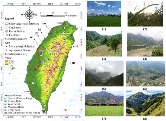
Figure 1.
Study area and field sites: distribution of topography, the target catchment, forestry stations, and monitoring stations, along with in situ photos of field sites 1 to 8. These photos illustrate land use and vegetation across an elevation gradient (generally from low to high), labeled (1–8) and corresponding to the details in Table 1.
Geographically, Taiwan spans elevations from sea level to 3952 m, and covers a total area of 35,873 square kilometers. The island stretches approximately 394 km in length and 144 km in width, centrally located at 23°58′N and 120°58′E. About two-thirds of Taiwan’s land area is mountainous, while the remaining one-third consists of flatlands, offering a wide range of ecosystems and climatic conditions. The Central Mountain Range (annotated as (a) in Figure 1), characterized by towering peaks and dense forests, plays a critical role in the island’s ecological diversity. Flanking this central spine are the eastern and western hill regions at mid-elevations (annotated as (b) and (c) in Figure 1). Typical flatland areas include mountain basins, urban basins, and the East Longitudinal Valley (annotated as (d) to (f) in Figure 1). Taiwan’s altitudinal gradients create distinct climate zones, transitioning from tropical climates at lower elevations to boreal forests at higher altitudes. This results in a diverse range of ecosystems, including tropical, subtropical, warm temperate, temperate, and boreal forests. The representative tree species across these various elevations are shown in Figure 1 and Table 1. Taiwan’s geographical setting exposes it to a variety of climatic and ecological conditions.

Table 1.
Locations and landscape characteristics of the field sites.
The forests of Taiwan host a diverse array of species, including Chamaecyparis formosensis (Taiwan red cypress), Chamaecyparis taiwanensis (Taiwan hinoki), Tsuga chinensis (Taiwan hemlock), Zelkova serrata (Japanese zelkova), Magnolia compressa (Formosan michelia), Cinnamomum kanehirae (Taiwan cinnamon), and Fraxinus griffithii (Griffith’s ash). According to the 1995 Taiwan Forest Resources and Land Use Survey, forests cover 2,102,400 hectares, accounting for 58.5% of the island’s total area. Forest composition includes 53.3% broad-leaved forests, 20.9% coniferous forests, 18.6% mixed coniferous and broad-leaved forests, and 7.2% bamboo forests. Taiwan is home to 30 forestry stations, 83% of which are managed by government agencies and 17% by academic institutions. Most stations are located in the foothill and high mountain regions, with only two situated in flatland areas.
Focusing on the LULC in the study area, this region encompasses Taiwan’s highest peak, Mt. Jade (3952 m), and five sub-catchments, collectively representing 37% of Taiwan’s forestry stations. This area provides a critical foundation for comprehensive assessments of vegetation, water dynamics, and land use at the catchment scale. To characterize the land use and vegetation distribution, we analyzed the Sentinel-2-based LULC data and the Sentinel-3-derived NDVI data from 2017 (Figure 2a,b). The LULC classification system included the following five major categories: Built area, River, Trees, Crops, and Bare ground. These categories capture the diverse land use patterns shaped by Taiwan’s unique topography and climatic conditions. As shown in Figure 3, trees dominate the island’s LULC, covering 66%, with built areas accounting for 17%, primarily in the urban lowlands. Crops, bare ground, and rivers make up the remainder, reflecting agricultural and hydrological features. In the study catchments, tree coverage rises to 79%, highlighting the presence of dense forests. These forests are key to ecological stability and hydrological regulation. The NDVI analysis shows that tree-dominated areas consistently have higher values, indicating healthy, dense vegetation, while the built areas and bare ground show lower NDVI values due to limited vegetation. These patterns provide essential baseline data for evaluating vegetation health and landscape dynamics.
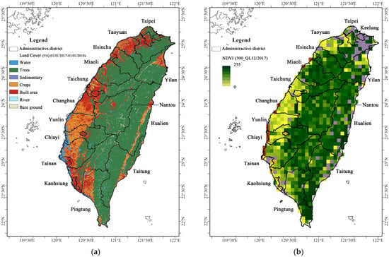
Figure 2.
Distribution of land use and land cover (LULC) types and normalized difference vegetation index (NDVI) values across Taiwan: (a) Spatial land use distribution based on the Sentinel-2 LULC in 2017, (b) NDVI values derived from the Sentinel-3-based NDVI_QL_201712 dataset.

Figure 3.
Percentage of LULC across Taiwan and the study areas.
2.2. Study Flow Chart and Data Acquisition
As summarized in Table 2, the existing dew estimation methods vary in terms of complexity, data requirements, and spatial applicability. Remote sensing approaches are typically applied at regional to global scales, whereas energy balance and empirical models typically require detailed input parameters, limiting their broader applicability. In Taiwan (Figure 1), data from 20 meteorological stations located in urban and high-mountain areas are suitable for use in empirical modeling. Meanwhile, 14 agricultural stations located in crop-targeted plains and hilly regions provide the detailed data required for energy balance models. Both types of stations provide essential meteorological variables, including temperature, dew point, and relative humidity.
Table 2.
Summary of the dew assessment methods, including their requirements, spatial coverage, and limitations.
Given the challenges of incorporating diverse terrain and data availability across all stations, this study employed a combined data-driven and theoretical approach to address key research gaps—particularly the difficulty of assessing the AMC in data-scarce regions. As illustrated in the methodological flow chart (Figure 4), the approach involved comparing the outputs of empirical dew models to estimate site-specific dew yield. The methodology also integrated remote sensing, meteorological observations, and environmental datasets to support sustainable land and ecological management strategies. This integrated methodology represents a significant step forward in aligning natural hydrometeorological processes with data-informed environmental decision-making.

Figure 4.
The flow chart illustrates the methodology of this study, integrating remote sensing, meteorological, and GIS data to analyze spatiotemporal variability and implications for the LULC patterns, environmental dynamics, ecological monitoring, and management prioritization strategies. Data sources: Meteorological data from the Central Weather Administration (CWA): https://opendata.cwa.gov.tw/index (accessed on 16 June 2025); Remotely sensed data, including the leaf area index (LAI), NDVI, and LULC, from the Land Monitoring Service, Copernicus: https://land.copernicus.eu/en (accessed on 16 June 2025) and Esri, Microsoft, and Impact Observatory: https://livingatlas.arcgis.com/landcoverexplorer/ (accessed on 16 June 2025); Landsat imagery from EarthExplorer, United States Geological Survey (USGS): https://earthexplorer.usgs.gov/ (accessed on 16 June 2025); ASTER GDEM from Jet Propulsion Laboratory, National Aeronautics and Space Administration (NASA): https://asterweb.jpl.nasa.gov/gdem.asp (accessed on 16 June 2025) or Japan Space Systems: https://www.jspacesystems.or.jp/ersdac/GDEM/E/ (accessed on 16 June 2025); Geological data from the Geological Survey and Mining Management Agency (GSMMA): https://hydro.geologycloud.tw/map (accessed on 16 June 2025).
Data acquisition relied on publicly available sources, including meteorological observations, remote sensing imagery, and geospatial datasets. These datasets were processed and analyzed to develop spatial indices and models that addressed several core research dimensions. The analytical framework consisted of four key components. First, the AMC potential was interpreted using kriging interpolation and compared with site-specific dew yield derived from empirical dew model results. Second, the condensation potential driven by vegetation was assessed using the LAI, referred to as the LAI-derived condensation potential (LCP). Third, land management suitability was evaluated through spatial analysis and pairwise correlations of the LULC types, resulting in the management suitability score (MSS) and management suitability prioritization (MSP). Finally, the GWP was estimated as a comparative baseline for validating the MSP outcomes across the different LULC categories.
This study integrated remote sensing data with GIS-based spatial analysis to generate comprehensive insights across the following three key domains: (1) the spatiotemporal variability of the AMC and their influence on the LULC dynamics; (2) the monitoring of environmental and hydrological variables essential for informed decision-making; and (3) the support of ecological resilience and climate adaptation strategies. The framework quantifies how vegetation influences dew formation, clarifying its significance in ecological processes and guiding sustainable land management priorities.
2.3. Fundamental Principles
2.3.1. Psychrometric Chart and Condensation
Temperature and relative humidity are fundamental parameters for characterizing the properties of moist air. The psychrometric chart (Figure 5) graphically depicts the physical and thermal characteristics of moist air, including temperature difference (ΔT = Ta − Td) and vapor pressure deficit (VPD), in relation to the driving force toward saturation curve [53,54,55]. It serves as a critical tool for interpreting atmospheric moisture conditions and assessing the potential for dew formation and condensation. In the context of this study, it facilitates the visualization of the relationships among air temperature, dew point temperature, relative humidity, and the condensation pathway.

Figure 5.
The psychrometric chart graphically depicts the physical and thermal characteristics of moist air, including temperature difference (ΔT = Ta − Td) and vapor pressure deficit (VPD = 100% − RH), in relation to the driving force toward saturation curve [53,54,55].
The saturation curve, which forms the uppermost boundary of the chart, represents air at 100% relative humidity. Any point along this curve indicates fully saturated air, where condensation is imminent. The dry-bulb temperature (Ta), shown along the horizontal axis, is the ambient air temperature measured with a standard thermometer. Lines of constant relative humidity (RH) curve from the dry-bulb axis toward the saturation curve, ranging from 0% to 100%, enabling the identification of moisture levels at varying temperatures. On the right-hand vertical axis is the humidity ratio (w), also known as specific humidity, which represents the mass of water vapor per unit mass of dry air. Diagonal lines sloping downward to the right indicate the wet-bulb temperature (Tw), which reflects the minimum temperature achievable through evaporative cooling. The dew point temperature (Td) is the temperature at which air becomes saturated (RH = 100%) and condensation begins. It is represented by horizontal lines extending leftward from the saturation curve. Additionally, enthalpy (h) lines, which slope diagonally upward to the right on the psychrometric chart, represent the total heat content of moist air. Enthalpy includes both sensible heat, associated with changes in the air temperature, and latent heat, associated with the moisture content. While these lines are commonly utilized in heating, ventilation, and air conditioning applications to estimate energy loads for heating, cooling, humidification, and dehumidification, they are equally valuable in atmospheric studies. In the context of this research, enthalpy lines are used to track energy changes during phase transitions, particularly condensation. As moist air cools and approaches saturation, the latent heat released during the condensation process becomes an important indicator of atmospheric stability and energy exchange.
2.3.2. Thermodynamic Principles and Key Formulas
This study evaluates condensation potential by integrating fundamental thermodynamic relationships that govern moisture phase transitions.
The Clausius–Clapeyron relationship describes the rate at which the saturation vapor pressure increases with the temperature. This thermodynamic principle governs the phase transition between liquid water and water vapor, and is expressed as follows:
where is the saturation vapor pressure (Pa), which represents the maximum moisture the air can hold at a given temperature before condensation occurs, denotes the latent heat of vaporization (J/kg), referring to the energy required to convert liquid water into vapor without a change in temperature, represents the specific gas constant for water vapor, approximately 461 J/kg·K, and T is the absolute temperature measured in Kelvin (K).
This relationship is fundamental in atmospheric sciences and hydrology, as it quantifies the exponential increase in the air’s moisture-holding capacity with rising temperature. It explains why warmer air can sustain more water vapor, thereby influencing dew formation, cloud development, and overall climate feedback processes.
In addition, the saturation vapor pressure (es) is the maximum vapor pressure that the air can hold at a given temperature. It is calculated using the Clausius–Clapeyron relation (or simplified Magnus-type formula) as follows [56]:
where T is the air temperature in °C.
Actual vapor pressure (e) is derived from the dew point temperature (Td), and relative humidity (RH) relates the actual vapor pressure to the saturation vapor pressure. It provides an important link between dew point, air temperature, and atmospheric moisture conditions.
2.4. Atmospheric Moisture Condensation
2.4.1. Nocturnal Condensation Potential Index
The condensation threshold, the temperature difference (ΔT = Ta − Td), and the VPD play a critical role in this study. It can be determined using the psychrometric chart (Figure 5), which visually illustrates the relationship between moist air properties toward saturation. The ΔT, defined as the difference between air temperature (Ta) and dew point temperature (Td), and the VPD, calculated as the difference between the saturated and actual vapor pressure at a given temperature, are key indicators of atmospheric moisture status. Lower values of the ΔT or VPD indicate sub-saturated conditions and, as these values approach zero, the air nears saturation, signaling a higher potential for condensation.
Since both key parameters (i.e., ΔT and VPD) are used to characterize the atmospheric moisture state, they can be jointly analyzed to derive a slope analogous to the tangent of the saturation curve. This slope represents the derivative at a given point, and reflects the instantaneous rate of change in the air’s moisture-holding capacity with respect to temperature. As the air temperature and humidity increase, the slope of the saturation curve becomes steeper, corresponding to higher enthalpy and vapor content, thereby enhancing the potential for dew formation. In this framework, variations in the slope between the ΔT and the VPD serve as indicators of site-specific condensation potential. A steeper slope implies a more rapid approach toward saturation under nocturnal cooling, signifying a higher potential for atmospheric moisture condensation.
The nightly condensation potential under precipitation-free conditions was quantified by proposing the Nocturnal Condensation Potential Index (NCPI). This index is derived from the linear relationship between the ΔT and the VPD at each meteorological station, based on daily mean values calculated during nighttime periods (22:00 to 06:00 local time). The resulting regressions consistently demonstrated high R2 values, confirming strong linearity across stations and enabling reliable characterization of the local condensation dynamics. To account for the seasonal variability in condensation behavior, Taiwan’s climate was divided into two distinct periods: the warm season (May to October) and the cold season (November to April of the following year), based on an approximate air temperature threshold of 21 °C. This classification enables a comparative analysis of seasonal trends in condensation potential and enhances the interpretability of the NCPI across different climatic regimes.
where f’(Ta) denotes the derivative of the saturation curve at Ta and a represents the slope of the linear regression, defined as the NCPI.
For normalization, the NCPI values are scaled between 0 and 1 using min–max scaling across all observations:
where amin and amax represent the minimum and maximum slope values observed across all stations, used to normalize the NCPI (denoted as NCPInorm, ranging from 0 to 1).
Higher normalized NCPI values indicate more favorable atmospheric conditions for nocturnal condensation, whereas lower values suggest greater atmospheric resistance to condensation. This framework provides a practical approach for assessing the condensation potential in regions such as Taiwan, where meteorological data are relatively limited but environmental management priorities require reliable spatial and temporal assessments.
2.4.2. Kriging Interpolation of the NCPI
Kriging is a geostatistical interpolation technique that estimates values at unsampled locations based on the spatial correlation of observed data points. It assumes that the spatial structure of the variable can be described by a variogram model. In this study, the normalized NCPI values derived from Equation (8) were used to construct empirical variograms. Three theoretical models—spherical, exponential, and Gaussian—were tested to fit the empirical variogram and assess spatial dependence. The key variogram parameters include the following: (1) Sill: the plateau of the variogram, representing the total variance; (2) Range: the distance at which the variogram reaches the sill, indicating the limit of spatial correlation; (3) Nugget: the value at the origin, accounting for measurement error or microscale variability. The best-fitting model was examined based on leave-one-out cross-validation (LOOCV), with the root mean square error (RMSE) used as the performance metric. The chosen model was then applied to generate continuous spatial estimates of the NCPI over a regular grid.
where is the observed value and is the predicted value.
2.4.3. Empirical Dew Model
The nightly dew yield rate (dh/dt) was estimated using Equation (10) to enable a comparison with the spatial patterns derived from the kriging interpolation of the NCPI [28,30]. The model assumes that dew condensation occurs on a planar surface with perfect emissivity (ε = 1). Sky emissivity, influenced by cloud cover and elevation, was computed using Equation (11) to account for its effect on long wave radiation and, consequently, on dew formation.
where and represent dew point and air temperatures (°C), N denotes 10 scales of cloud cover (oktas) in this study, u stands for wind velocity (m/s), SE denotes sky emissivity, and H represents elevation (m).
2.5. LAI-Derived Condensation Potential and Management Suitability
Atmospheric vapor condenses on various vegetative surface areas acting as a prominent medium due to its extensive surface area. Previous studies have primarily assessed the leaf wetness and the LWP at local scales. However, when evaluating patterns at the regional scale, the availability of suitable meteorological data and remote sensing observations is often limited. Despite these constraints, identifying priority areas for management remains essential. This study proposes an approach to address this challenge by integrating the normalized NCPI values with the LAI to derive the LCP, as defined in Equation (12). The original LAI values, which can typically exceed 5 or 6 in dense vegetative areas, were normalized to a 0–1 range to ensure consistency and comparability with the other indices used in the derivation of the MSS. This normalization facilitates the integration of multiple datasets into a unified framework while preserving spatial variability patterns relevant for identifying management priority zones.
It is important to note that the LCP represents a potential estimation; the actual dew yield on vegetation, including processes such as absorption and interception by leaves, remains unknown and will be the focus of future research. Nevertheless, identifying regions with high condensation potential is crucial for guiding funding allocation and management interventions. To further support prioritization efforts, we introduced the MSS, a composite metric that emphasized the areas where climatic conditions were suboptimal but the ecological potential was strong. The MSS is defined as follows:
In this formulation, the term (1 − NCPInorm) reflects the weather gap from optimal conditions, while the LAI captures the site’s biological responsiveness. Areas characterized by a high NCPI value (indicating strong climatic suitability) but a low LAI value (reflecting limited ecological potential) tend to exhibit lower MSS values, thereby signaling higher MSP for targeted interventions. Conversely, areas with higher MSS values correspond to lower MSP values, suggesting reduced urgency for active management. The schematic interpretation of the LCP, MSS, and MSP levels is summarized in Table 3. It is noteworthy that relying solely on the LCP may lead to misleading conclusions. For example, although two cases may both exhibit moderate LCP values, their MSS values may differ significantly—one indicating a high MSP and the other a low priority. This comparison highlights that the MSS more effectively captures the combined effects of climatic suitability and ecological potential, providing a more reliable framework for guiding management decisions.
Table 3.
Schematic interpretation of the LAI-derived condensation potential (LCP) and management suitability prioritization (MSP) levels based on climate and ecological potential. Threshold criteria are detailed in the results section.
The development of the MSP framework reflects the principles of equity and efficiency in resource allocation, emphasizing the areas where interventions are both necessary and likely to yield effective outcomes. It follows the structure of multi-criteria decision-making models widely adopted in sustainability research, where prioritization is determined by the overlap of ecological opportunity and management demand. The MSS values enable standardized comparisons across spatial units and support integration into spatial decision-support systems and GIS-based analytical workflows. To facilitate interpretation and application, the MSS results were classified into four priority levels—High, Moderate–High, Moderate, and Low—using the natural breaks (Jenks optimization) method [57]. This classification offers a robust basis for informing management strategies in forest conservation, afforestation planning, and drought response.
2.6. Pairwise Correlation of the LULC
A pairwise correlation analysis of the LULC categories was conducted to apply the MSS and MSP framework to the LULC evaluation. Specifically, we analyzed data from six consecutive seasons corresponding to the same time periods within the study area. For each LULC type, the following statistical indicators were calculated: mean value, standard deviation (std), and coefficient of variation (Cv) for the LAI, NCPI, and MSS. In addition, Pearson correlation coefficients (r-values) were calculated between the LAI and the NCPI, and between the LAI and the MSS, to assess their linear relationships. The statistical formulas used in this analysis are as follows:
where and are the observed values of the two variables, and are the mean values of x and y, n is the number of observations and is the standard deviation.
The mean and standard deviation provide basic descriptions of the data’s central tendency and spread, while the coefficient of variation (Cv) offers a normalized measure of variability relative to the mean. The Pearson correlation coefficient quantifies the strength and direction of linear relationships between variables. This analysis enables the identification of the LULC categories where vegetation structure (represented by the LAI), climatic condensation potential (represented by the NCPI), and management priority (represented by the MSP) exhibit strong or weak interactions. Understanding these relationships is crucial for optimizing land management strategies, prioritizing interventions, and enhancing the effectiveness of resource allocation in environmental planning and conservation efforts.
2.7. Groundwater Potential as a Comparative Baseline
The MSS and MSP were developed in this study to evaluate the suitability of the LULC management based on atmospheric moisture dynamics and vegetation responsiveness. To ensure that the MSS reflects surface ecological and atmospheric conditions rather than broader hydrological processes, the GWP was introduced as an independent comparative baseline. The hydrological cycle inherently links atmospheric, surface, and subsurface water processes. However, given that the MSS is derived from nocturnal atmospheric condensation potential and vegetation indices, it is theoretically independent of groundwater dynamics. By contrast, the GWP specifically characterizes subsurface hydrological properties. Therefore, a lack of correlation between the MSS and the GWP would validate that the MSS captures surface–atmosphere–vegetation interactions pertinent to the LULC management, rather than reflecting groundwater availability. This comparison is essential to confirm the intended specificity of the MSS, and to ensure that its impact on the LULC assessment is not confounded by unrelated hydrological factors.
To perform this validation, a synthesized GWP map was generated by integrating RS and GIS datasets at a spatial resolution of 30 m × 30 m. The parameters used in this analysis include lineament density (LD), soil moisture index (SMI) derived from Landsat imagery, slope degree (SD), drainage density (DD), and the topographic wetness index (TWI) calculated from a digital elevation model (DEM). Additionally, hydrogeological units (HGU) were incorporated, reflecting the spatial complexity of geological structures and lithology in Taiwan.
As shown in the flow chart (Figure 4), the primary datasets and post-processed outputs utilized in this study are essential for estimating the GWP. The steps are as follows. In the geological data, a digital geological map at a 1:50,000 scale detailing geological sections and rock types is used to delineate the HGU. This helps in identifying the structural and lithological characteristics of the study area. In the DEM analysis, the DEM, provided by the ASTER GDEM, was processed using ArcGIS 10.2 (Esri, Redlands, CA, USA). A spatial analysis was performed to calculate the TWI and the SD.
where represents the upslope contributing area per unit contour length, and is the slope gradient (degree or radians).
To compute the DD, the flow accumulation (FA) method was applied. The maximum, mean, and standard deviation values of the FA in the study area were found to be 1,461,926, 1017, and 23,682, respectively. By adjusting the threshold for the FA, it was determined that a threshold value of 8046, resulting in five stream orderings, yielded the clearest representation of the favorable groundwater distribution.
where represents the length of the drainage and A is the unit of area.
Landsat imagery captured on multiple dates (6 November 1994; 9 June 2015; 2 December 2015; 27 June 2016; 4 December 2016) was analyzed to derive the land surface temperature (LST), NDVI, and SMI using the band math tool in ENVI 5.3 (Exelis Visual Information Solutions, Boulder, CO, USA). The SMI was defined by Equation (20) based on the scatter plot of the LST and NDVI values forming a trapezoid in the LST–NDVI space. Consequently, the standard deviation in the above four seasons of the SMI results were compiled statistics for the SMI thematic map.
where Ts max and Ts min are the maximum and minimum surface temperature for a given NDVI value, respectively. These values were obtained by a linear regression of known remotely-sensed data for both dry and wet edges in the LST–NDVI space.
To improve the LD map, a principal component analysis (PCA) was applied to the imagery from 6 November 1994, enhancing the image processing and facilitating the extraction of relevant features. Geological lineaments were then extracted using the LINE module of PCI Geomatica 2013 (PCI Geomatics, Richmond Hill, ON, Canada). The parameters for this extraction, such as the radius of the filter in pixels, threshold for edge gradient, threshold for curve length, threshold for line fitting error, threshold for angular difference, and threshold for linking distance, were established based on the literature [50] and Table 4. Geological lineaments longer than 1000 m were considered significant, with artificial features excluded from the analysis. The resulting lineament density map was then generated as follows:
where represents the length of the lineament and A is the unit of area.
Table 4.
List of parameter values used in the LINE module of PCI Geomatics for automatic lineament extraction in this study.
Finally, these multi-parameter datasets were ranked using the Jenks natural breaks method, producing groundwater potential values on a scale from 1 to 5. GIS overlay tools were applied to accumulate and normalize these values from 0 to 1, delineating the potential groundwater zones that reflect the complex interplay between geological and hydrological features.
3. Results
3.1. Spatiotemporal Dynamics of the NCPI, LAI, and MSS
3.1.1. NCPI and Kriging Interpolation
Based on the meteorological data, Taiwan’s seasons were categorized into two distinct periods: the warm season (May to October) and the cold season (November to April of the following year), using an air temperature threshold of approximately 21 °C. This seasonal division is illustrated in Figure 6, based on data from the representative meteorological stations located in northern, central, and southern Taiwan during the period 2016–2017. The NCPI, calculated for both the warm and cold seasons, exhibited slight but consistent differences, and reflected variations in the nocturnal condensation potential as visualized through the psychrometric relationships (Figure 5).
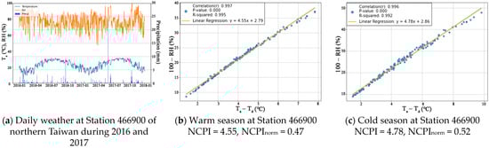
Figure 6.
Time series meteorological data and the seasonal NCPI values at the represented stations of northern, central, and southern Taiwan from 2016 to 2017.
The spatiotemporal patterns of the NCPI were investigated by analyzing data from monitoring stations across Taiwan over six consecutive seasons—three cold and three warm—spanning from November 2016 to October 2019. The raw NCPI values ranged from 2.61 to 6.75, and were normalized to NCPInorm values between 0 and 1. Despite spatial gaps due to the uneven station distribution across Taiwan’s complex terrain, kriging interpolation enabled the generation of continuous NCPInorm maps, facilitating seasonal spatial pattern analysis (Figure 7). For interpolation, an empirical variogram was constructed, and three theoretical models—spherical, exponential, and Gaussian—were tested. The best-fitting model was examined based on LOOCV, using the root mean square error (RMSE) as the performance criterion. The variogram parameters, including sill, range, and nugget, along with the RMSE values, are presented in Table 5. The spherical model was selected as the most appropriate due to its applicability in scenarios where the semivariance increases rapidly and then levels off—consistent with the behavior of the NCPI data. The RMSE values ranged from 0.0703 to 0.1032, indicating satisfactory interpolation accuracy.
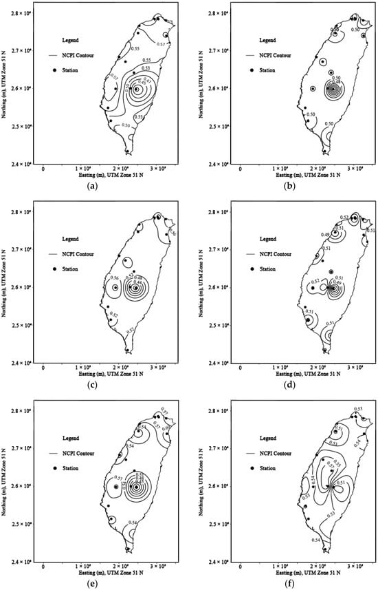
Figure 7.
Seasonal kriging map of NCPInorm: (a) cold season between November 2016 and April 2017; (b) warm season between April 2017 and October 2017; (c) cold season between November 2017 and April 2018; (d) warm season between April 2018 and October 2018; (e) cold season between November 2018 and April 2019; (f) warm season between April 2019 and October 2019.
Table 5.
Variogram models and the root mean square error (RMSE) for the kriging interpolation of NCPInorm.
Seasonal variation in the variogram range suggests that the spatial autocorrelation distance tends to be longer during the cold season. The nugget effect, ranging from 30% to 60% of the sill, implies a moderate measurement error or short-range variability in the data. The interpolated NCPI maps revealed distinct seasonal and regional patterns. Broader and more spatially uniform NCPI distributions were observed in some periods (e.g., the first cold season; Figure 7a), while others displayed more localized clustering and sharper gradients (e.g., the third warm season; Figure 7f). Regional disparities were also evident, with higher NCPI values consistently found in high-altitude areas, aligning with the previous research that reported increased dew formation at higher elevations [19,30,33,34]. Furthermore, the temporal shifts in the NCPI between seasons highlighted the dynamic interactions among elevation, seasonal temperature changes, and nocturnal moisture condensation processes. These findings underscore the strong influence of seasonal climate patterns on condensation potential across Taiwan’s diverse topography.
3.1.2. Distribution and Classification of the LAI
The mean LAI across Taiwan was analyzed over six periods—three cold seasons and three warm seasons from 2016 to 2019—building upon the seasonal patterns identified in the NCPI. The monthly LAI data were averaged to assess both the spatial and temporal variability for each season. The LAI values were categorized into four classes using the Jenks natural breaks method: low, moderate, moderate–high, and high. The threshold values (0.31, 0.54, and 0.76) were derived from the combined mean LAI across all six seasons (Table 6).
Table 6.
Categorization of the mean LAI values across Taiwan into four classes based on the Jenks natural breaks method.
In line with the previous recommendations emphasizing catchment-scale analysis [5,9,52], this study focused on the catchment areas to better capture the nuanced spatial and seasonal variations. The LAI distribution maps and histograms (Figure 8) revealed distinct seasonal patterns. Within the study catchment, the LAI histograms displayed a single pronounced peak (Figure 8), shifting from approximately 0.6 during the cold season to around 0.8 during the warm season. Given that approximately 79% of the catchment is covered by trees (Figure 3), the histograms were heavily skewed toward higher LAI values. During the cold seasons, low to moderate LAI values were mainly observed in the central mountain range, likely reflecting seasonal dormancy, reduced vegetation activity, or snow cover in the higher-altitude zones. By contrast, a slight increase in the LAI during the warm seasons was evident, particularly across mid-altitude regions, driven by enhanced vegetation growth under favorable climatic conditions. In the hilly areas adjacent to the central mountains and the western hills, moderate LAI values prevailed during the cold seasons, influenced by resilient vegetation and moderate climatic conditions. By contrast, the eastern hills consistently exhibited high LAI values across all seasons, reflecting abundant year-round precipitation from the northeast monsoons, plum rains, and typhoons. The urbanized areas and plains exhibited predominantly low LAI values. However, the western coastal plains demonstrated a notable seasonal increase in the LAI from the cold to the warm season, largely associated with the agricultural crop cycles.
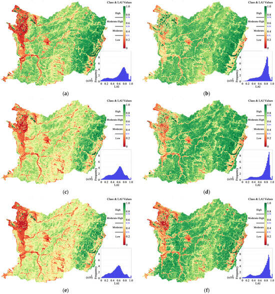
Figure 8.
Seasonal distribution of the LAI classes and histograms of the LAI values in the study catchment: (a) cold season between November 2016 and April 2017; (b) warm season between April 2017 and October 2017; (c) cold season between November 2017 and April 2018; (d) warm season between April 2018 and October 2018; (e) cold season between November 2018 and April 2019; (f) warm season between April 2019 and October 2019.
Overall, these findings highlighted the complex interactions among terrain, land use, vegetation dynamics, and seasonal climatic factors across Taiwan. The observed spatial patterns of the LAI provided important insights into ecosystem health, agricultural productivity, and regional microclimate regulation.
3.1.3. Identification of Management Suitability Prioritization
The MSS, a composite metric integrating (1 − NCPI) and LAI, was implemented to effectively prioritize areas for management intervention. This approach enables management strategies to accurately identify areas where plant water requirements persist, even after accounting for the supplemental water potential provided by leaf surface condensation. By combining both metrics, this method more realistically reflects management needs, focusing on improving insufficient vegetation biomass and enhancing atmospheric moisture condensation. It highlights regions that, although favorable in terms of weather, may suffer from inadequate vegetation, thereby impairing overall ecosystem health. Thus, the MSS provides a more reliable assessment of land management suitability across Taiwan. In this framework, lower MSS values correspond to higher MSP (i.e., areas requiring more immediate intervention), whereas higher MSS values indicate lower MSP (i.e., relatively stable or resilient areas). The MSP values were classified into four categories using the Jenks natural breaks method: High, Moderate–High, Moderate, and Low, with the corresponding MSS thresholds of 0.15, 0.27, and 0.37, respectively, derived from the mean values across six seasons (Table 7).
Table 7.
Categorization of the MSP across Taiwan into four classes based on the Jenks natural breaks method.
The results showed that the seasonal patterns of the MSS were more distinctly defined compared to those of the NCPI or the LAI alone. High to moderately high MSP values (i.e., lower MSS values) predominated along the western slopes of the Central Mountain Range during the cold seasons, expanding into mid-altitude hill regions between 2017 and 2019. By contrast, moderate MSP levels dominated most regions during the warm seasons, although the hill areas adjacent to the Central Mountain Range exhibited a shift from moderately high to high MSP between 2017 and 2019. In the eastern hills, low MSP levels persisted across all seasons but showed a slight increase toward moderate levels during the warm season of 2019. During the cold seasons, areas of high and moderate-high MSP extended up to elevations of approximately 2000 m, likely influenced by mountain–valley wind systems circulating below ridge heights (~2000 m a.s.l.), as described by [58]. Above this elevation, the prevailing winds maintained lower MSP levels (i.e., higher MSS values) from the northeast to southeast within the mixed coniferous and broad-leaved forests (Figure 1(7)). In the urbanized areas and plains, high MSP regions expanded along the river systems toward the mountainous areas during the cold seasons. During the warm seasons, high MSP zones became particularly evident across the coastal plains, indicating a significant reduction in dew formation potential and increased management needs.
The spatial extent of low MSP (i.e., high MSS) areas was limited to specific regions, suggesting that favorable conditions for land management suitability were both environmentally and seasonally constrained. During the warm season of 2017, low MSP levels were predominantly observed in the eastern hills, an area characterized by robust vegetation cover and favorable climatic conditions (Figure 9b). This pattern coincided with periods of abundant precipitation from plum rains and typhoons, which supported sustained vegetation water demand and enhanced atmospheric moisture condensation potential. In 2018, portions of the Central Mountain Range also exhibited low MSP levels during both the cold and warm seasons (Figure 9c,d), reflecting the combined influence of stable vegetation cover, lower temperatures, and adequate humidity—conditions conducive to nocturnal condensation. However, a progressive shift toward higher MSP values was observed over time. By 2019, the regions exhibiting low MSP levels had become increasingly scarce, particularly across the western hills and portions of the Central Mountain Range. This trend suggests an increasing sensitivity of vegetation to seasonal climatic variations, potentially driven by shifts in temperature, moisture availability, or land cover changes. Factors such as vegetation stress, environmental degradation, and climatic variability may have contributed to the observed rise in the MSP values, indicating a growing need for more targeted management strategies in the future.
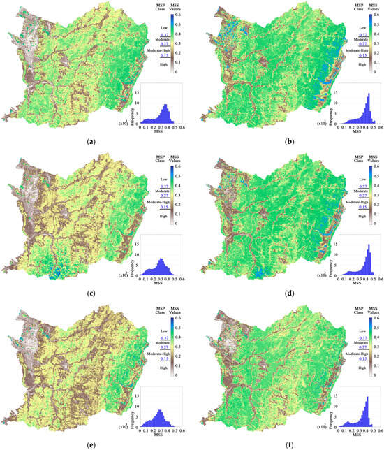
Figure 9.
Seasonal distribution of the MSP classes and histograms of the MSS values in the study catchment: (a) cold season between November 2016 and April 2017; (b) warm season between April 2017 and October 2017; (c) cold season between November 2017 and April 2018; (d) warm season between April 2018 and October 2018; (e) cold season between November 2018 and April 2019; (f) warm season between April 2019 and October 2019.
3.2. Pairwise Correlation and Plot Visualizations of the LULC Metrics
We conducted statistical analyses using the pairwise Pearson correlations and the MSP visualizations to better understand the characteristics of the LAI, NCPI, and MSP across different LULC types in Taiwan. The statistical comparisons of these indices for the various LULC categories during the cold and warm seasons from 2016 to 2019 are summarized in Figure 10. The key findings within the study catchment are detailed as follows. The pairwise correlation analysis (Figure 10) revealed that trees consistently exhibit the highest mean LAI, while built areas and rivers display greater variability (higher Cv) across periods. Furthermore, the NCPI fluctuated significantly in trees and bare ground between November 2017 and April 2018, particularly when analyzed at the catchment scale using mean values. A box plot analysis (Figure 11) highlighted an increasing trend in the slope degrees across the five LULC categories within the catchment.
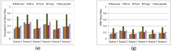
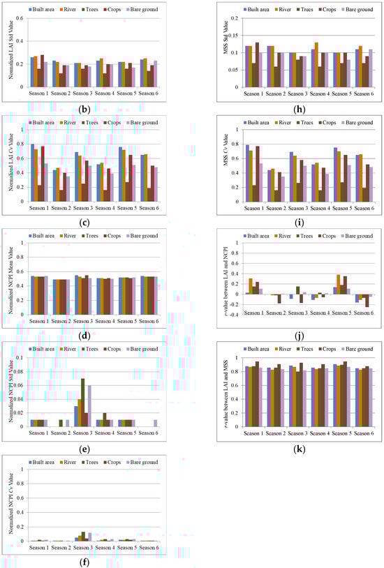
Figure 10.
Plot of six continuous seasons corresponding to the same time periods delineated in Figure 7 for the target catchment, along with the statistical values for each LULC: (a) normalized LAI mean value; (b) normalized LAI std value; (c) normalized LAI Cv value; (d) normalized NCPI mean value; (e) normalized NCPI std value; (f) normalized NCPI Cv value; (g) MSS mean value; (h) MSS std value; (i) MSS Cv value; (j) r-value between the LAI and NCPI; (k) r-value between the LAI and MSS.

Figure 11.
The box plot shows the distribution of the MSS across five LULC categories over six periods in the target catchment. The MSS variability among the LULC types provides insights for the MSP decisions.
We used river plots based on the first quartile, mean, and third quartile statistics to further explore the temporal dynamics in the vegetation and climatic patterns (Figure 12). These plots provided insights into trends, variability, central tendencies, and simplified interpretations. This study divided six periods of the LCP mean values into five sections: November 2016 to April 2017, April 2017 to October 2017, October 2017 to April 2018, April 2018 to October 2018, and October 2018 to October 2019. For tree and bare ground types, the first, third, and fifth sections showed an increasing slope transition from cold to warm seasons, with slightly lower intercepts, indicating relative stabilization. Conversely, for the built areas, rivers, and crops, the slopes decreased in the first, third, and fifth sections. The interquartile range (IQR) was wider in the first section but narrowed in the fifth, indicating reduced variability over time. However, these categories also demonstrated a concerning decrease in the MSS values. These findings underscore the importance of river plots for analyzing climate trends and informing forest management practices. This method demonstrated broader potential applications in climate change studies and ecological monitoring.
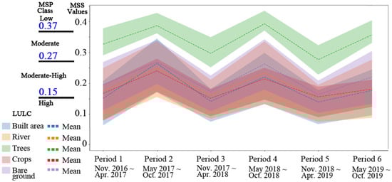
Figure 12.
The river plot visualizes and reveals the dynamic patterns of the MSS, highlighting the evolution of statistical indicators over time. Within each LULC class, these plots identify periods of increased climatic variability or stability. The mean line tracks central trends across periods, enabling the detection of significant shifts. By combining these elements—mean, first quartile, and third quartile—the river plots provide a clearer understanding of temporal and categorical dynamics at the catchment scale.
3.3. Temporal MSS Changes and Empirical Dew Yield of Field Sites in LULUCF Areas
Since the MSS was derived from the LAI, a correlation between the two was expected. However, the results showed that this relationship was not straightforward, especially in the tree-dominated areas where canopy structure complexity may weaken the direct correlation. The correlation coefficients (r-values) between the LAI and the MSS, measured from November 2016 to October 2019 (Figure 10k), for different LULC types in the study catchment were as follows: built areas (0.88), rivers (0.86), trees (0.86), crops (0.93), and bare ground (0.85). Although the tree-dominated areas showed higher mean MSS values and lower coefficients of variation (Cv), the relationship between the LAI and the MSS in these areas is weaker. This is likely due to saturation effects in the canopy structure; trees typically have high LAI values, and beyond a certain threshold, increases in the LAI may have less influence on the MSS. Additionally, trees have more complex canopy structures with multiple layers, variations in leaf angles, and shading effects, which further weaken the direct correlation between the LAI and the MSS. By contrast, the other LULC types, such as crops, exhibit a stronger and more direct relationship between the LAI and the MSS (r = 0.93), due to simpler canopy structures.
The MSS data were extracted from eight field sites to further investigate this funding with varying locations, tree types, and elevations (Figure 13). Field site 1 is in urban and crop landscapes, while sites 2 to 8 are situated in mountainous LULUCF areas. Over the warm and cold seasons, field sites 1 and 7 showed minimal change in the MSS, while sites 3 to 8 in the LULUCF areas experienced significant variation, particularly during the cold seasons. Notably, field site 7, located in the eastern hills, exhibited higher MSS values than those in the western hills across both seasons. This regional variation reflects the influence of both biophysical and external drivers on condensation potential.
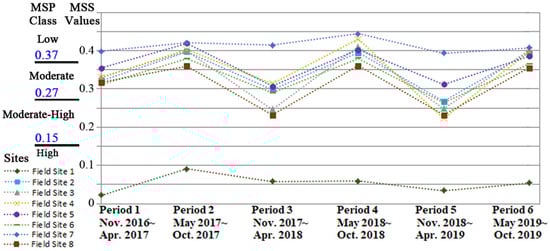
Figure 13.
The seasonal variation of the MSS at field sites, with notable changes in the land-use, land-use change, and forestry (LULUCF) areas (Field sites 2, 3, 4, 5, 6, and 8 in Figure 1), demonstrated that, despite the same LULC type, the MSS varied across each site, highlighting spatiotemporal changes.
In particular, the western hill sites (e.g., sites 4, 5, and 6) experienced pronounced declines in the MSS during the cold season, likely influenced by seasonal drought events and reduced vegetation activity [13,14]. Furthermore, land use changes, such as the partial conversion of natural forest to fruit tree orchards at field site 6, introduce anthropogenic pressures that may lower the LAI and disrupt canopy structure, further decreasing the MSS. These findings highlight that both climatic stress (e.g., drought) and human-induced land cover changes contribute to spatial and temporal shifts in the MSS. As a result, the MSS of site 1 remained below 0.1 (indicating high MSP), while the others ranged from 0.2 to 0.45. This suggests that the MSP can serve as a valuable tool for prioritizing land use and vegetation management strategies, especially in regions subject to environmental and anthropogenic stressors.
Dew yield estimates were derived using Equation (10) at two representative sites to compare the MSP findings with the empirical dew data. Field site 1 and field site 5 are located near meteorological stations 467490 and 467650, respectively. Seasonal NCPI values and corresponding average dew yields for these stations are presented in Figure 14 and Figure 15. Station 467490 (near field site 1) exhibited consistently lower dew yields, whereas station 467650 (near field site 5) demonstrated higher condensation potential. This indicates that field site 5 had a stronger dew formation capacity and therefore a lower MSP classification than field site 1, supporting the utility of combining field observations with empirical and remote-sensing data for robust site assessment.
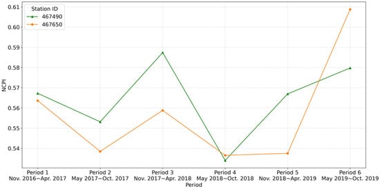
Figure 14.
The seasonal variation of the NCPI at meteorological stations 467490 and 467650 near field site 1 and 5.
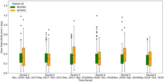
Figure 15.
The seasonal variation of dew yield at meteorological stations 467490 and 467650 near field site 1 and 5.
3.4. Validation of the MSS Independence Using GWP
We analyzed the relationship between the MSS and the LULC using the GWP as a comparative baseline, given that the hydrological cycle governs the movement of water between the atmosphere, land surface, and groundwater systems. However, the MSS should not be directly related to the GWP. Therefore, we created thematic maps for each parameter (Figure 16a–f), with the synthesized GWP map shown in Figure 16g. The GWP values, ranging from 0 to 1, were classified into the following four levels using natural break criteria: low (0.20–0.50), medium (0.50–0.56), high (0.56–0.63), and very high (0.63–0.97). The percentage distribution of these groundwater potential levels was 26% (low), 15% (medium), 32% (high), and 27% (very high). According to the literature [50], areas with a groundwater yield exceeding 60 L per minute, suitable for local and regional water supplies, correspond to regions classified as very high potential (0.63–0.97 GWP).
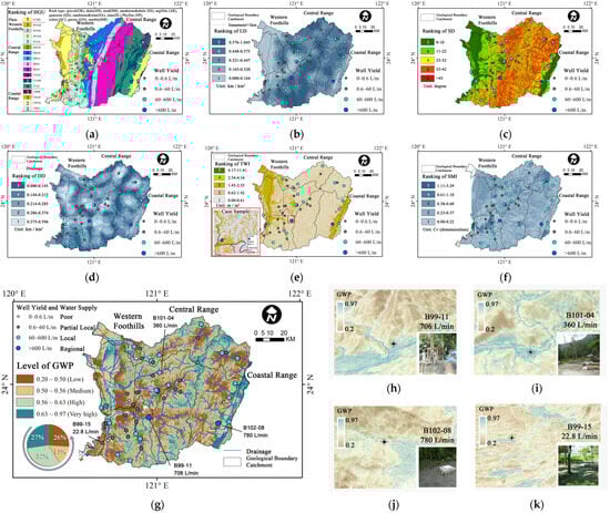
Figure 16.
The thematic maps of groundwater potential map: (a) hydrogeological unit (HGU); (b) lineament density (LD); (c) slope degree (SD); (d) drainage density (DD); (e) topographic wetness index (TWI); (f) soil moisture index (SMI) as multi-period analysis results of coefficient of variation; (g) synthesized groundwater potential (GWP) map; (h) Station B99-11 located in High–Very High GWP of convergence of two rivers with the yield of 706 L per minute; (i) Station B101-4 between High–Very High GWP of concave and convex mountains with the yield of 360 L per minute; (j) Station B102-8 located in High–Very High GWP of the mouth of two mountains with the yield of 780 L per minute; (k) Station B99-15 located in low GWP area with gentle strata and terrain and the yield of only 22.8 L per minute.
People have identified groundwater resources based on topographic features and personal experience during earlier agricultural periods, when scientific data was limited. This reliance on observational knowledge led to the development of traditional proverbs and folk practices related to groundwater exploration. When paired with the 3D GWP thematic maps (Figure 16h–k), the significance of such traditional knowledge becomes clear. We analyzed four specific terrains to validate these classifications, comparing the results with in situ pumping test data. For instance, at the convergence of two rivers, the yield was 706 L per minute at Station B99-11. In the area between concave and convex mountains, the yield was 360 L per minute at Station B101-4. In the mouth of two mountains, the yield was 780 L per minute at Station B102-8. In the gentle strata and terrain, the yield was only 22.8 L per minute at Station B99-15. These results highlight the effectiveness of the GWP classifications in identifying groundwater potential sites.
We applied a similar approach after validating the availability of the GWP classes and analyzed the seasonal variations in the MSS across each GWP class (Figure 17). In the very high GWP class, the mean MSS values were lower, but the IQR was larger, indicating greater variability. By contrast, the low GWP class exhibited higher mean MSS values with a smaller IQR. Although the mean MSS values were similar across the GWP classes, showing minimal variation, the values differed significantly among the LULC types. Additionally, the mean MSS values during the warm season were higher than in the cold season, which aligned with the results observed in the LULC analysis regarding the seasonal factors. Therefore, the MSS was strongly influenced by the LULC, and the GWP served as a useful comparative baseline to validate these findings.

Figure 17.
The box plot illustrates the distribution of the MSS across four GWP categories over six distinct periods in the study area. The MSS is strongly influenced by the LULC, as shown in Figure 11. Thus, the GWP serves as a useful comparative baseline to validate these findings.
4. Discussion
4.1. Implications of the MSS Dynamics for Ecosystem Management
This study highlights the critical role of vegetation density, meteorological conditions, and the LULC characteristics in influencing the LAI-derived atmospheric moisture condensation potential, called the LCP. A deeper understanding of the LCP dynamics offers practical insights across multiple sectors. In agriculture, it supports the optimization of dew harvesting and irrigation planning in regions with limited access to conventional water resources [18,30]. In hydrology, it provides a valuable tool for evaluating the atmospheric water resource potential of areas with low precipitation [22]. Moreover, for ecosystem management, identifying regions with high condensation potential is crucial for sustaining local biodiversity and maintaining ecosystem resilience. Collectively, these findings contribute to more sustainable land-use practices and resource management strategies, particularly in areas where dew represents a significant ecological and hydrological resource [19,25,37]. Importantly, this study highlights the pronounced seasonal dynamics in the MSS, with lower values observed during colder seasons compared to warmer periods. These seasonal variations help identify critical zones for understanding the ecological and climatic factors that regulate dew formation [2,3,9]. The integration of the MSS with land use and climatic data thus provides a valuable framework for identifying management priorities, guiding targeted interventions, and optimizing land-use planning according to seasonal variations in atmospheric moisture dynamics.
The MSS developed in this study was specifically designed to evaluate the suitability of the LULC management based on atmospheric moisture dynamics and vegetation responsiveness, independent of broader subsurface hydrological processes. To validate this independence, the GWP was introduced as an external baseline. The absence of a direct relationship between the MSS and the GWP confirms that the MSS predominantly reflects surface ecological and atmospheric conditions on the LULC rather than groundwater-driven processes. This strengthens the reliability of using the MSS in surface-based land management evaluations. Nevertheless, certain vegetation types inevitably rely on groundwater resources, leading to complex interactions. Although the mean MSS is lower in regions with high GWP, the broad IQR observed (Figure 17) suggests substantial variability. High GWP zones, often located in recharge areas at higher altitudes or discharge zones along riverbeds, exhibit LAI patterns with significant seasonal variability. By contrast, low GWP regions, typically situated on slopes with established tree cover, tend to show more stable LAI dynamics. As a result, prioritization based solely on the GWP is not feasible, as moderate MSP levels prevail across different groundwater settings. Furthermore, while groundwater availability influences vegetation health and the LAI, and by extension the MSS, the relationships are complex and warrant further investigation.
We found that the MSS values in the river and crop areas declined over the time evaluating the MSS as a proxy for ecosystem monitoring, as shown in Figure 11 and Figure 12. The decreasing MSS trends may indicate increasing environmental stress, leading to reduced supplemental water availability for the LWP. Under such conditions, plants relying on foliar water uptake struggle to sustain physiological functions [15,59,60], often developing coping mechanisms, such as reducing the LWP [11]. These trends may be associated with drought events or shifts in climate patterns, as evidenced by Taiwan’s severe droughts in 2020 and 2021. Lower MSS values were observed particularly in central and southern Taiwan during the cold (dry) seasons. (Figure 9a,c,e). This pattern is consistent with findings from remote sensing and satellite-derived indices, such as temperature–soil moisture dryness indices, which have proven effective in monitoring agricultural drought stress and water availability [13,14]. Although Taiwan generally receives abundant rainfall, seasonal water shortages still occur, largely due to high evaporation rates during dry months, thereby adversely affecting agriculture, domestic water supply, and industrial activities.
Overall, this study underscores the importance of understanding the MSS dynamics for advancing sustainable ecosystem management. By identifying areas of high or vulnerable atmospheric moisture potential, the MSS offers an innovative dimension for prioritizing land-use planning and ecosystem conservation efforts.
4.2. Limitations and Future Research
Several limitations were identified in this study, each pointing to opportunities for future work. First, the use of the 2017 LULC data as a baseline may not fully capture the dynamic nature of land-use alterations over time. Incorporating multi-year LULC datasets would offer a more comprehensive understanding of long-term trends and their influence on hydrological and ecological processes. Second, the limited availability of meteorological stations, particularly those equipped with dew-point measurements, constrains the accuracy of the condensation assessment. Although agricultural stations are available in some regions, they often lack the critical parameters needed for a comprehensive analysis. Expanding meteorological monitoring networks would improve spatial coverage and data quality, enhancing the reliability of the NCPI and MSS estimations. Third, the current formulation of the LCP does not yet incorporate important vegetation traits, such as leaf surface roughness or species-specific water absorption capacities. These factors could significantly influence condensation efficiency and should be integrated into future models to improve the quantitative accuracy.
Currently, the application of the MSS facilitates the identification of additional vegetation characteristics that are crucial for optimizing land management strategies. Although the method is designed to maximize spatial coverage through remote sensing and minimal in situ meteorological validation, future applications should adopt a two-tiered framework as follows: first, using the MSS to identify priority regions, and second, conducting targeted field investigations to validate and refine the management strategies. This tiered approach would significantly enhance the operational applicability of the MSS-guided land-use policies. In the long term, the MSS and MSP could become a strategic governance tool, enabling the scientifically validated prioritization of interventions for more effective and efficient landscape management.
Future research should also explore incorporating high-MSP zones into land-use planning to mitigate the impacts of climate variability on forest health, photosynthetic activity, carbon emissions, and related environmental issues. Investigating the relationship between the LCP and other environmental parameters—such as soil moisture, evapotranspiration, and precipitation patterns—would deepen our understanding of condensation dynamics under changing climatic conditions. Expanding the temporal scope to include long-term datasets could reveal more robust trends in the LCP as an indicator of climate change. Additionally, integrating natural processes with engineered solutions, such as condensation-enhancing materials or structures, may optimize water yields in the high-NCPI zones. Finally, incorporating high-resolution vegetation and hydrological indices into predictive models would improve our understanding of landscape–climate interactions and contribute to the development of sustainable forest health management strategies.
5. Conclusions
This study presented a novel application of the NCPI to assess key atmospheric condensation indicators, including temperature and relative humidity, using a psychrometric chart-based approach. This method offered an alternative means of dew assessment in data-scarce regions by linking leaf surface condensation with plant water demand—an increasingly vital factor as climate change intensifies aridity. The research also introduced the MSS as a reliable indicator for monitoring forest health and supporting adaptive land management strategies. This study revealed significant variations in the management priorities across seven regions classified under the LULUCF framework, even among areas sharing the same land cover types. This finding underscored the utility of the LCP as a practical tool for evaluating micro-meteorological conditions and vegetation dynamics. The integration of remote sensing with limited meteorological data provided a cost-effective framework for ecological monitoring and land-use planning in water-stressed environments, enabling informed decision-making where traditional data collection is constrained. The broader implications of this study suggest that coupling natural processes with technological tools can support more resilient land management strategies in the face of climate variability. The proposed two-tiered framework—using the MSS to identify priority zones followed by field-based validation—enhanced the practical applicability of remote-sensing-based tools for policy development (e.g., forest conservation, drought mitigation, land restoration).
Author Contributions
Conceptualization, J.-J.L. and A.N.A.; methodology, J.-J.L. and A.N.A.; software, J.-J.L.; validation, J.-J.L. and A.N.A.; formal analysis, J.-J.L. and A.N.A.; investigation, J.-J.L.; resources, J.-J.L.; data curation, J.-J.L.; writing—original draft preparation, J.-J.L.; writing—review and editing, A.N.A.; visualization, J.-J.L.; supervision, A.N.A.; project administration, J.-J.L.; funding acquisition, A.N.A. All authors have read and agreed to the published version of the manuscript.
Funding
This research received no external funding.
Data Availability Statement
Data are available in a public, open access repository.
Acknowledgments
This study gives thanks to the database support from the Central Weather Administration, Geological Survey and Mining Management Agency, and remotely sensing imagery support from ESA, NASA, JPL, JSS, Esri, and the EU Copernicus programme, contributing to this study’s completeness.
Conflicts of Interest
Author J.-J.L. was employed by the company Sinotech Engineering Consultants, Inc. The remaining authors declare that the research was conducted in the absence of any commercial or financial relationships that could be construed as a potential conflict of interest.
Abbreviations
The following abbreviations are used in this manuscript:
| AMC | Atmospheric moisture condensation |
| ASTER GDEM | Advanced Spaceborne Thermal Emission and Reflection Radiometer Global Digital Elevation Model |
| CWA | Central Weather Administration |
| DD | Drainage density |
| DEM | Digital elevation model |
| FA | Flow accumulation |
| GIS | Geographic information system |
| GWP | Groundwater potential |
| GSMMA | Geological Survey and Mining Management Agency |
| HGU | Hydrogeological units |
| IQR | Interquartile range |
| LAI | Leaf area index |
| LCP | LAI-derived condensation potential |
| LD | Lineament density |
| LOOCV | Leave-one-out cross-validation |
| LULC | Land use and land cover |
| LULUCF | The land-use, land-use change, and forestry |
| LST | Land surface temperature |
| LWP | Leaf water potential |
| MSS | Management suitability score |
| MSP | Management suitability prioritization |
| NASA | National Aeronautics and Space Administration |
| NCPI | Nocturnal condensation potential index |
| NDVI | Normalized difference vegetation index |
| PCA | Principal component analysis |
| RH | Relative humidity |
| RMSE | Root mean square error |
| RS | Remote sensing |
| SD | Slope degree |
| SMI | Soil moisture index |
| TWI | Topographic wetness index |
| USGS | United States Geological Survey |
| VPD | Vapor pressure deficit |
References
- Tenkanen, M.K.; Tsuruta, A.; Tyystjärvi, V.; Törmä, M.; Autio, I.; Haakana, M.; Tuomainen, T.; Leppänen, A.; Markkanen, T.; Raivonen, M.; et al. Using atmospheric inverse modelling of methane budgets with Copernicus land water and wetness data to detect land use-related emissions. Remote Sens. 2024, 16, 124. [Google Scholar] [CrossRef]
- Cheng, H.; Park, C.Y.; Cho, M.; Park, C. Water requirement of urban green infrastructure under climate change. Sci. Total Environ. 2023, 893, 164887. [Google Scholar] [CrossRef]
- Wu, H.; Long, B.; Huang, N.; Lu, N.; Qian, C.; Pan, Z.; Men, J.; Zhang, Z. Impacts of climate change on ecological water use in the Beijing–Tianjin–Hebei region in China. Water 2024, 16, 319. [Google Scholar] [CrossRef]
- Bock, A.D.; Belmans, B.; Vanlanduit, S.; Blom, J. Alvarado-Alvarado, A.A.; Audenaert, A. A review on the leaf area index (LAI) in vertical greening systems. Build. Environ. 2023, 229, 109926. [Google Scholar] [CrossRef]
- Gao, Z.; Chen, Y.; Zhang, Z.; Duan, T.; Chen, J.; Li, A. Continuous leaf area index (LAI) observation in forests: Validation, application, and improvement of LAI-NOS. Forests 2024, 15, 868. [Google Scholar] [CrossRef]
- Gavilán-Acuna, G.; Coops, N.C.; Tompalski, P.; Mena-Quijada, P.; Varhola, A.; Roeser, D.; Olmedo, G.F. Characterizing annual leaf area index changes and volume growth using ALS and satellite data in forest plantations. Sci. Remote Sens. 2024, 10, 100159. [Google Scholar] [CrossRef]
- Wang, Y.; Fang, H. Derivation and Evaluation of LAI from the ICESat-2 data over the NEON sites: The impact of segment size and beam type. Remote Sens. 2024, 16, 3078. [Google Scholar] [CrossRef]
- Zhen, Z.; Chen, S.; Yin, T.; Chavanon, E.; Lauret, N.; Guilleux, J.; Henke, M.; Qin, W.; Cao, L.; Li, J.; et al. Using the negative soil adjustment factor of soil adjusted vegetation Index (SAVI) to resist saturation effects and estimate leaf area index (LAI) in dense vegetation areas. Sensors 2021, 21, 2115. [Google Scholar] [CrossRef]
- Cui, J.; Lian, X.; Huntingford, C.; Gimeno, L.; Wang, T.; Ding, J.; He, M.; Xu, H.; Chen, A.; Gentine, P.; et al. Global water availability boosted by vegetation-driven changes in atmospheric moisture transport. Nat. Geosci. 2022, 15, 982–988. [Google Scholar] [CrossRef]
- Reddy, P.S. Chapter 20—Breeding for Abiotic Stress Resistance in Sorghum. In Woodhead Publishing Series in Food Science, Technology and Nutrition, Breeding Sorghum for Diverse End Uses; Aruna, C., Visarada, K.B.R.S., Bhat, B.V., Tonapi, V.A., Eds.; Woodhead Publishing: Sawston, UK, 2019; pp. 325–340. [Google Scholar] [CrossRef]
- Diatta, A.A.; Min, D.; Jagadish, K.S.V. Chapter Two—Drought stress responses in non-transgenic and transgenic alfalfa—Current status and future research directions. Adv. Agron. 2021, 170, 35–100. [Google Scholar] [CrossRef]
- Hussain, M.; Farooq, S.; Hasan, W.; Ul-Allah, S.; Tanveer, M.; Farooq, M.; Nawaz, A. Drought stress in sunflower: Physiological effects and its management through breeding and agronomic alternatives. Agric. Water Manag. 2018, 201, 152–166. [Google Scholar] [CrossRef]
- Liou, Y.-A.; Thai, M.-T. Surface water availability and temperature (SWAT): An innovative index for remote sensing of drought observation. IEEE Trans. Geosci. Remote Sens. 2023, 61, 4507312. [Google Scholar] [CrossRef]
- Thai, M.-T.; Liou, Y.-A. Advancements in the temperature-soil moisture dryness index (TMDI) for drought monitoring in southwestern Taiwan. IEEE Trans. Geosci. Remote Sens. 2024, 62, 4405415. [Google Scholar] [CrossRef]
- Li, Z.-K.; Gong, X.-W.; Wang, J.-L.; Chen, Y.-D.; Liu, F.-Y.; Li, H.-P.; Lü, G.-H. Foliar water uptake improves branch water potential and photosynthetic capacity in Calligonum mongolicum. Ecol. Indic. 2023, 146, 109825. [Google Scholar] [CrossRef]
- Pinter, P.J., Jr. Effect of dew on canopy reflectance and temperature. Agric. For. Meteorol. 1986, 19, 187–205. [Google Scholar] [CrossRef]
- Gerlein-Safdia, C.; Koohafkan, M.C.; Chung, M.; Rockwell, F.E.; Thompson, S.; Caylor, K.K. Dew deposition suppresses transpiration and carbon uptake in leaves. Agric. For. Meteorol. 2018, 259, 305–316. [Google Scholar] [CrossRef]
- Alnaser, W.E.; Barakat, A. Use of condensed water vapour from the atmosphere for irrigation in Barhein. Appl. Energy 2000, 65, 3–18. [Google Scholar] [CrossRef]
- Kidron, G.J.; Herrnstadt, I.; Barzilay, E. The role of dew as a moisture source for sand microbiotic crusts in the Negev Desert, Israel. J. Arid Environ. 2002, 52, 517–533. [Google Scholar] [CrossRef]
- Duvdevani, S. Dew Gradients in relation to climate, soil and topography. In Proceedings of the International Symposium on Desert Research, Research Council of Israel, Jerusalem, Israel, 7–14 May 1952; Govt. Printer: Jerusalem, Israel, 1953; pp. 136–148. [Google Scholar]
- Lhomme, J.-P.; Jimenez, O.F. Estimating dew duration on banana and plantain leaves from standard meteorological observations. Agric. For. Meteorol. 1992, 62, 263–274. [Google Scholar] [CrossRef]
- Schmitz, H.F.; Grant, R.H. Precipitation and dew in a soybean canopy: Spatial variations in leaf wetness and implications for Phakopsora pachyrhizi infection. Agric. For. Meteorol. 2009, 149, 1621–1627. [Google Scholar] [CrossRef]
- Nilsson, T.M.J. Initial experiments on dew collection in Sweden and Tanzania. Sol. Energy Mater. Sol. Cells 1996, 40, 23–32. [Google Scholar] [CrossRef]
- Williams, D.W.; Powell, A.J., Jr.; Dougherty, C.T.; Vincelli, P. Separation and quantitation of the sources of dew on creeping bentgrass. Crop Sci. 1998, 38, 1613–1617. [Google Scholar] [CrossRef]
- Jacobs, A.F.G.; Heusinkveld, B.G.; Berkowicz, S.M. Dew deposition and drying in a desert system: A simple simulation model. J. Arid Environ. 1999, 42, 211–222. [Google Scholar] [CrossRef]
- Wilson, T.B.; Bland, W.L.; Norman, J.M. Measurement and simulation of dew accumulation and drying in a potato canopy. Agric. For. Meteorol. 1999, 93, 111–119. [Google Scholar] [CrossRef]
- Li, X.Y. Effects of gravel and sand mulches on dew deposition in the semiarid region of China. J. Hydrol. 2002, 260, 151–160. [Google Scholar] [CrossRef]
- Beysens, D.; Pruvost, V.; Pruvost, B. Dew observed on cars as a proxy for quantitative measurements. J. Arid Environ. 2016, 135, 90–95. [Google Scholar] [CrossRef]
- Vuollekoski, H.; Vogt, M.; Sinclair, V.A.; Duplissy, J.; Järvinen, H.; Kyrö, E.-M.; Makkonen, R.; Petäjä, T.; Prisle, N.L.; Räisänen, P.; et al. Estimates of global dew collection potential on artificial surfaces. Hydrol. Earth Syst. Sci. 2015, 19, 601–613. [Google Scholar] [CrossRef]
- Tomaszkiewicza, M.; Abou Najm, M.; Zurayk, R.; El-Fadela, M. Dew as an adaptation measure to meet water demand in agricultureand reforestation. Agric. For. Meteorol. 2017, 232, 411–421. [Google Scholar] [CrossRef]
- Atashi, N.; Rahimi, D.; Goortani, B.M.; Duplissy, J.; Vuollekoski, H.; Kulmala, M.; Vesala, T.; Hussein, T. Spatial and temporal investigation of dew potential based on long-term model simulations in Iran. Water 2019, 11, 2463. [Google Scholar] [CrossRef]
- Atashi, N.; Rahimi, D.; Al Kuisi, M.; Jiries, A.; Vuollekoski, H.; Kulmala, M.; Vesala, T.; Hussein, T. Modeling long-term temporal variation of dew formation in Jordan and its link to climate change. Water 2020, 12, 2186. [Google Scholar] [CrossRef]
- Muselli, M.; Lekouch, I.; Beysens, D. Physical and chemical characteristics of dew and rain in north-west Africa with focus on Morocco: Mapping past and future evolution (2005–2100). Atmosphere 2022, 13, 1974. [Google Scholar] [CrossRef]
- Muselli, M.; Beyens, D. Mapping past, present and future dew and rain water resources for biocrust evolution in southern Africa. J. Hydrol. Hydromech. 2021, 69, 400–420. [Google Scholar] [CrossRef]
- Lin, J.-J.; Arslan, A.N. Assessing the impact of land use on dew yield using remote sensing data in Taiwan. Int. Arch. Photogramm. Remote Sens. Spat. Inf. Sci. 2025, 48, 207–212. [Google Scholar] [CrossRef]
- Jia, Z.; Zhao, Z.; Zhang, Q.; Wu, W. Dew yield and its influencing factors at the Western Edge of Gurbantunggut Desert, China. Water 2019, 11, 733. [Google Scholar] [CrossRef]
- Aguirre-Gutiérrez, C.A.; Holwerda, F.; Goldsmith, G.R.; Delgado, J.; Yepez, E.; Carbajal, N.; Escoto-Rodríguez, M.; Arredondo, J.T. The importance of dew in the water balance of a continental semiarid Grassland. J. Arid Environ. 2019, 168, 26–35. [Google Scholar] [CrossRef]
- Binks, O.; Finnigan, J.; Coughlin, I.; Disney, M.; Calders, K.; Burt, A.; Vicari, M.B.; da Costa, A.L.; Mencuccini, M.; Meir, P. Canopy wetness in the Eastern Amazon. Agric. For. Meteorol. 2021, 297, 108250. [Google Scholar] [CrossRef]
- Cosh, M.H.; Kabela, E.D.; Hornbuckle, B.; Gleason, M.L.; Jackson, T.J.; Prueger, J.H. Observations of dew amount using in situ and satellite measurements in an agricultural landscape. Agric. For. Meteorol. 2009, 149, 1082–1086. [Google Scholar] [CrossRef]
- Heusinkveld, B.G.; Berkowicz, S.M.; Jacobs, A.F.G.; Hillen, W.; Holtslag, A.A.M. A new remote optical wetness sensor and its applications. Agric. For. Meteorol. 2008, 148, 580–591. [Google Scholar] [CrossRef]
- Xu, Y.; Dou, Y.; Yu, Y.; Yang, X. The dew particle interception abilities of typical plants in Northeast China plant leaves capture particles in dew. Adv. Meteorol. 2022, 2022, 7157012. [Google Scholar] [CrossRef]
- Madeira, A.C.; Kim, K.S.; Taylor, S.E.; Gleason, M.L. A simple cloud-based energy balance model to estimate dew. Agric. For. Meteorol. 1999, 111, 55–63. [Google Scholar] [CrossRef]
- Kuwagata, T.; Maruyama, A.; Kondo, J.; Watanabe, T. Theoretical study on dew formation in plant canopies based on a one-layer energy-balance model. Agric. For. Meteorol. 2024, 354, 109911. [Google Scholar] [CrossRef]
- Gillespie, T.J.; Brisco, B.; Brown, R.J.; Sofko, G.J. Radar detection of a dew event in wheat. Remote Sens. Environ. 1990, 33, 151–156. [Google Scholar] [CrossRef]
- Schneebeli, M.; Wolf, S.; Kunert, N.; Eugster, W.; Mätzler, C. Relating the X-band opacity of a tropical tree canopy to sapflow, rain interception and dew formation. Remote Sens. Environ. 2011, 115, 2116–2125. [Google Scholar] [CrossRef]
- Glanville, K.; Sheldon, F.; Butler, D.; Capon, S. Effects and significance of groundwater for vegetation: A systematic review. Sci. Total Environ. 2023, 875, 162577. [Google Scholar] [CrossRef]
- El-Hokayem, L.; De Vita, P.; Usman, M.; Link, A.; Conrad, C. Mapping potentially groundwater-dependent vegetation in the Mediterranean biome using global geodata targeting site conditions and vegetation characteristics. Sci. Total Environ. 2023, 898, 166397. [Google Scholar] [CrossRef]
- Nguyen, K.-A.; Liou, Y.-A. Global mapping of eco-environmental vulnerability from human and nature disturbances. Sci. Total Environ. 2019, 664, 995–1004. [Google Scholar] [CrossRef]
- Teodoro, A.C.; Duarte, L. Chapter 11—The synergy of remote sensing and geographical information systems in the management of natural disasters. In Micro and Nano Technologies, Nanotechnology-Based Smart Remote Sensing Networks for Disaster Prevention; Denizli, A., Alencar, M.S., Nguyen, T.A., Motaung, D.E., Eds.; Elsevier: Amsterdam, The Netherlands, 2022; pp. 217–230. [Google Scholar] [CrossRef]
- Lin, J.-J.; Liou, Y.-A. Integrating In-Situ Data and RS-GIS Techniques to Identify Groundwater Potential Sites in Mountainous Regions of Taiwan. Appl. Sci. 2020, 10, 4119. [Google Scholar] [CrossRef]
- Abera, K.A.; Gebreyohannes, T.; Abrha, B.; Hagos, M.; Berhane, G.; Hussien, A.; Belay, A.S.; Van Camp, M.; Walraevens, K. Vulnerability mapping of groundwater resources of Mekelle City and surroundings, Tigray region, Ethiopia. Water 2022, 14, 2577. [Google Scholar] [CrossRef]
- Ponette-González, A.G.; Brauman, K.A.; Marín-Spiotta, E.; Farley, K.A.; Weathers, K.C.; Young, K.R.; Curran, L.M. Managing water services in tropical regions: From land cover proxies to hydrologic fluxes. Ambio 2015, 44, 367–375. [Google Scholar] [CrossRef]
- Niu, G.; Kozai, T.; Sabeh, N. Chapter 11—Physical environmental factors and their properties. In Plant Factory, 2nd ed.; Kozai, T., Niu, G., Takagaki, M., Eds.; Academic Press: Cambridge, MA, USA, 2020; pp. 185–195. [Google Scholar] [CrossRef]
- Hundy, G.F.; Trott, A.R.; Welch, T.C. Chapter 19—Air and Water Vapour Mixtures. In Refrigeration, Air Conditioning and Heat Pumps, 5th ed.; Hundy, G.F., Trott, A.R., Welch, T.C., Eds.; Butterworth-Heinemann: Oxford, UK, 2016; pp. 301–312. [Google Scholar] [CrossRef]
- Alduchov, O.A.; Eskridge, R.E. Improved Magnus form approximation of saturation vapour pressure. J. Appl. Meteor. 1996, 35, 601–609. [Google Scholar] [CrossRef]
- Koutsoyiannis, D. Clausius–Clapeyron equation and saturation vapour pressure: Simple theory reconciled with practice. Eur. J. Phys. 2012, 33, 295. [Google Scholar] [CrossRef]
- Jenks, G.F. The data model concept in statistical mapping. Int. Yearb. Cartogr. 1967, 7, 186–190. [Google Scholar]
- Wang, C.-W. The Observation and Model Simulation of Valley Boundary Layer. Master’s Thesis, National Taiwan University, Taipei, Taiwan, 2011. [Google Scholar] [CrossRef]
- Tian, J.; Li, Z.; Wang, H.; Lv, G.; Li, W.; Wang, H.; Wang, Y. Physiological responses and ecological benefits of water uptake by Populus euphratica leaves in arid areas. Forests 2024, 15, 430. [Google Scholar] [CrossRef]
- Boanares, D.; Jovelina da-Silva, C.; Mary Dos Santos Isaias, R.; Costa França, M.G. Oxidative metabolism in plants from Brazilian rupestrian fields and its relation with foliar water uptake in dry and rainy seasons. Plant Physiol. Biochem. 2020, 146, 457–462. [Google Scholar] [CrossRef]
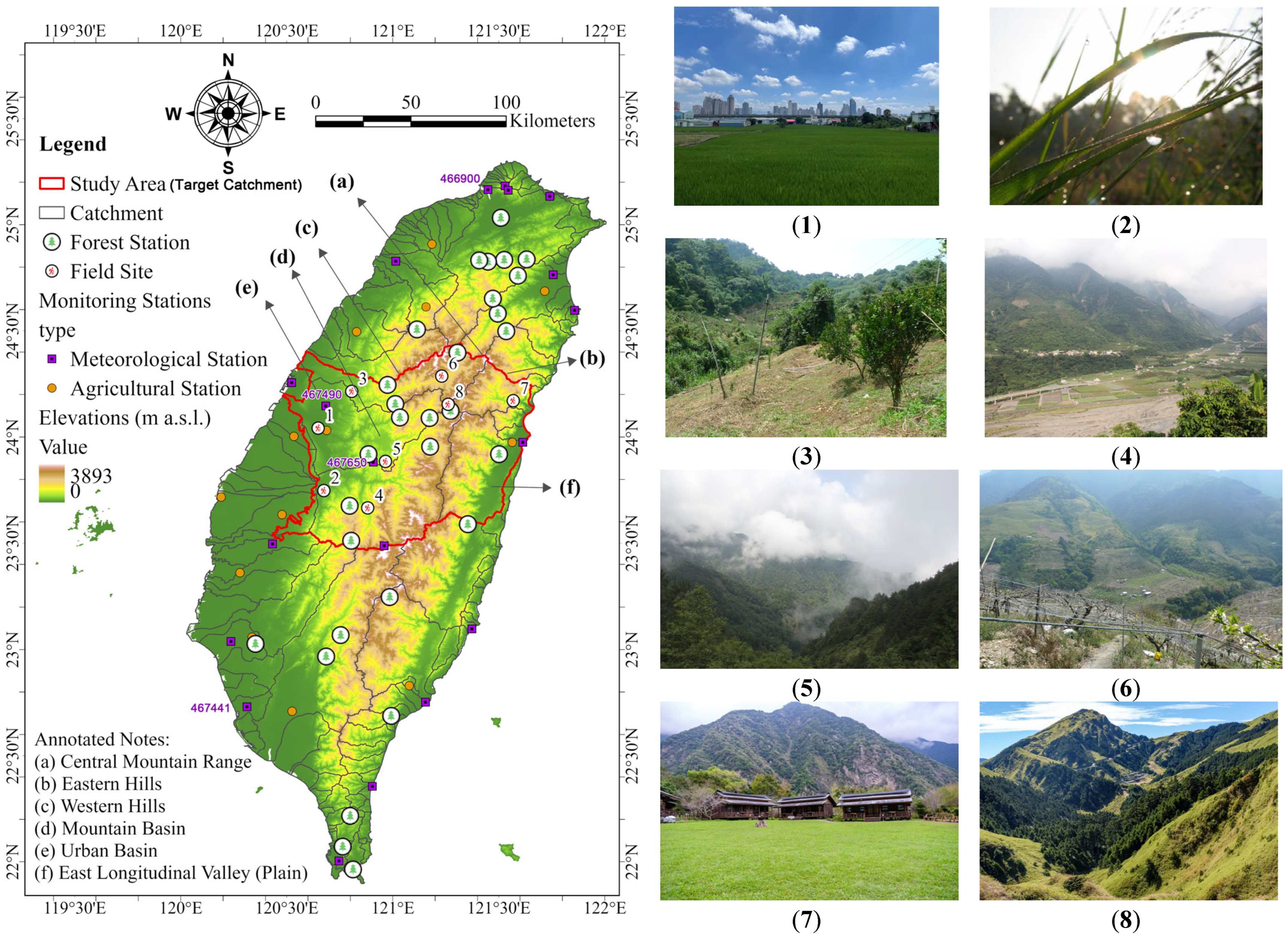

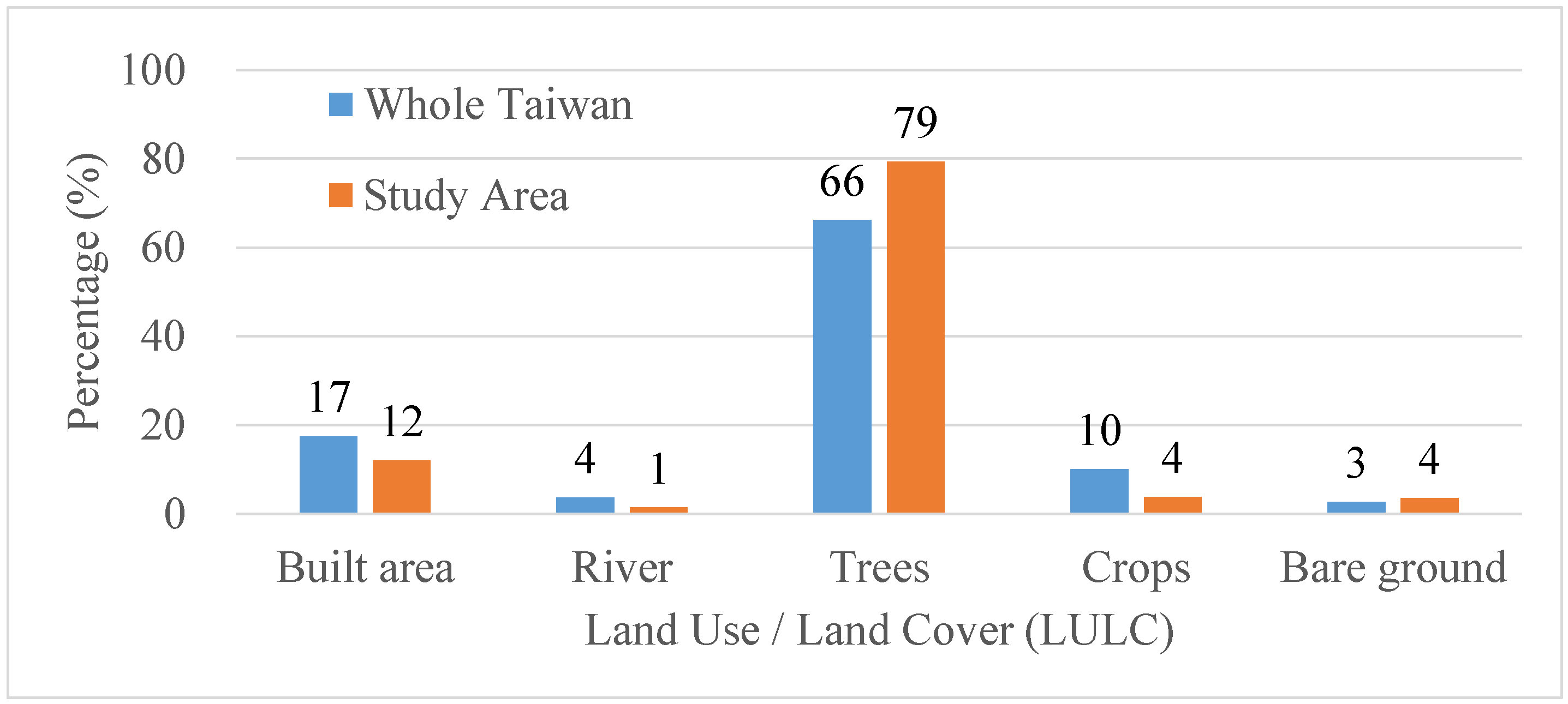
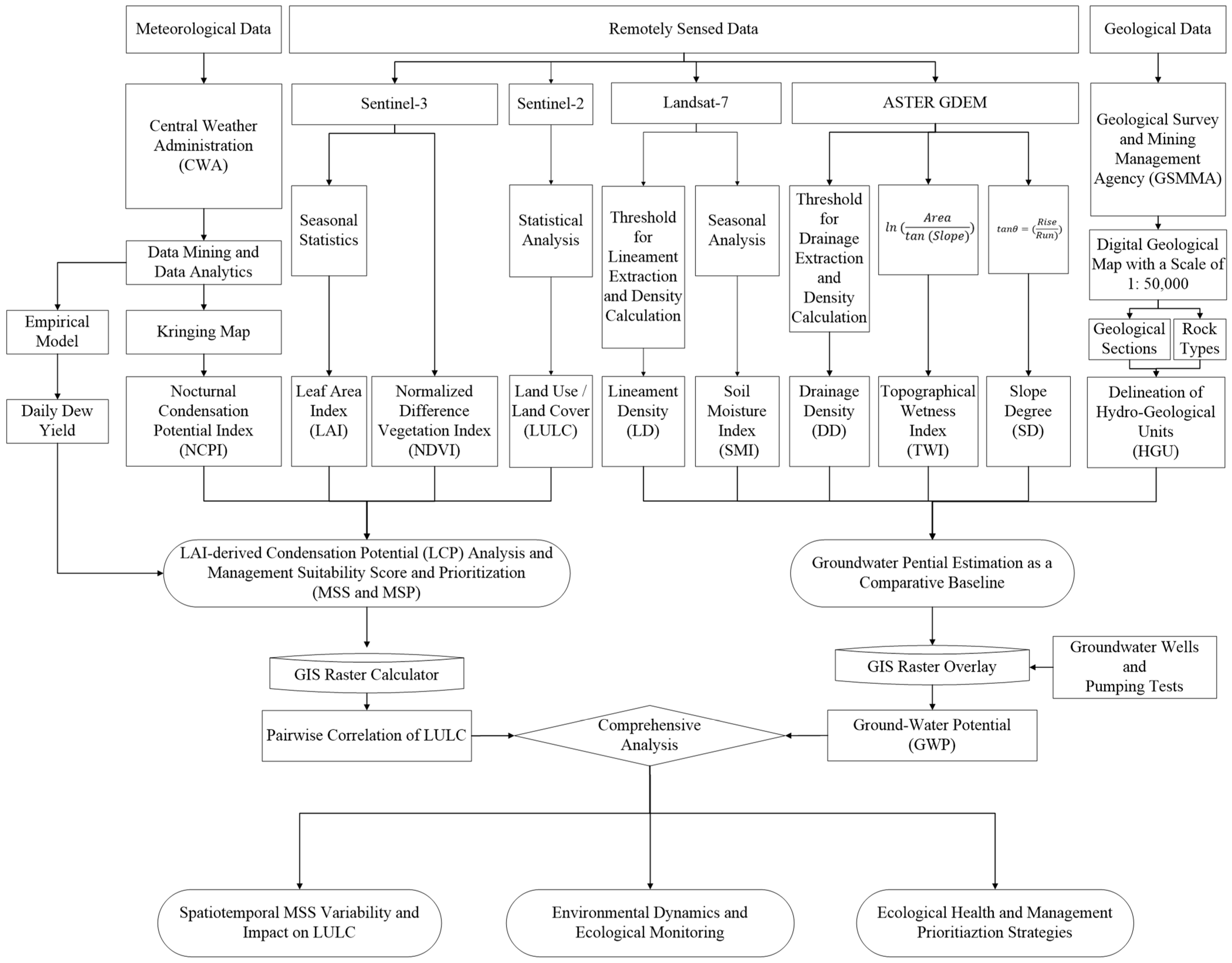
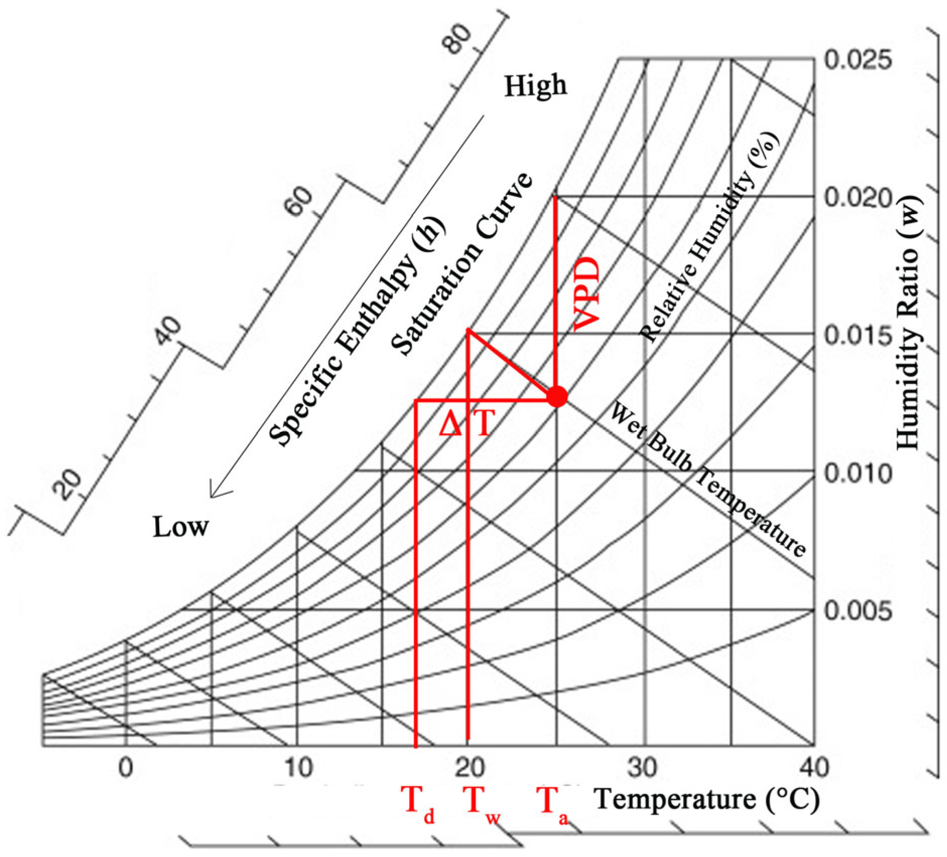

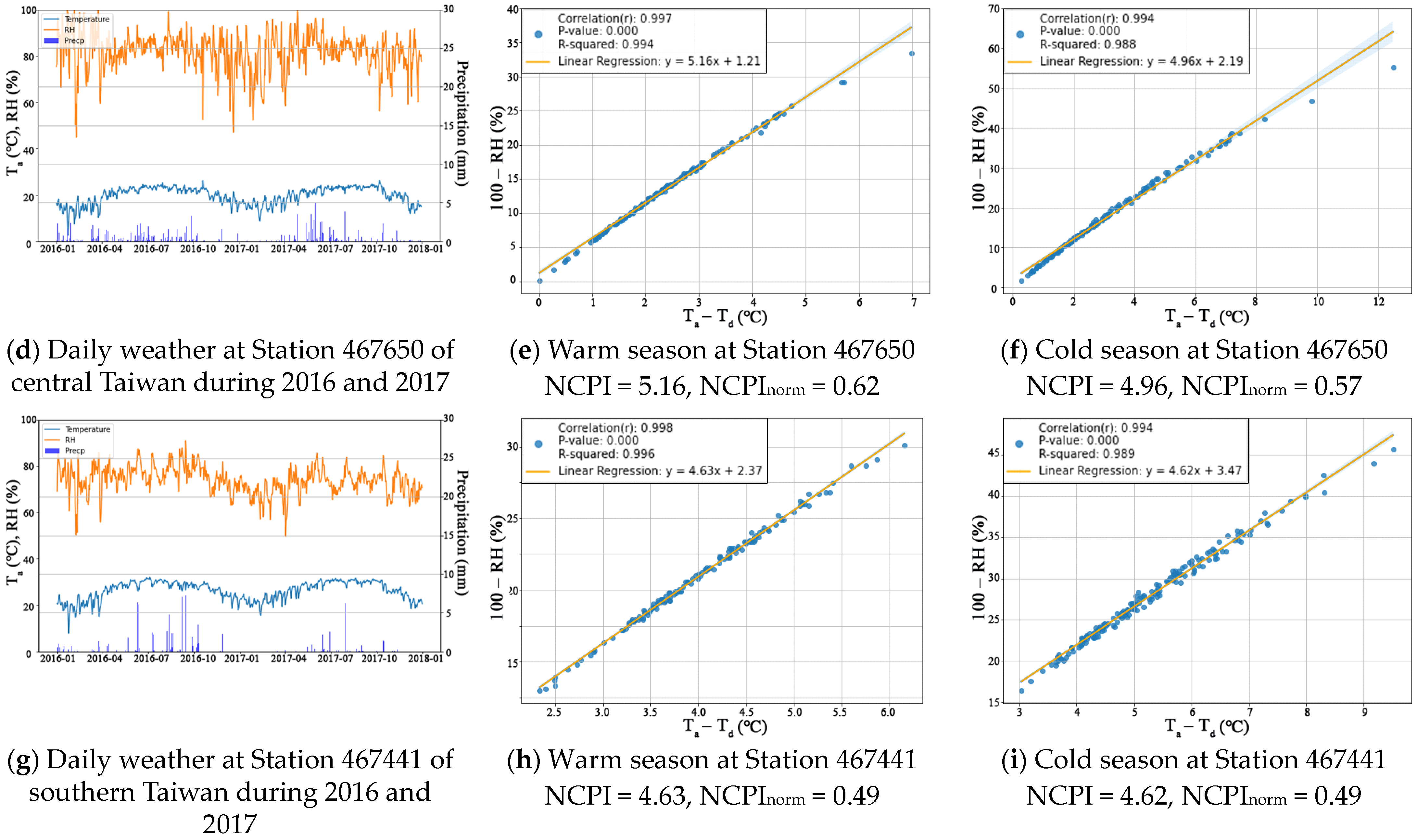


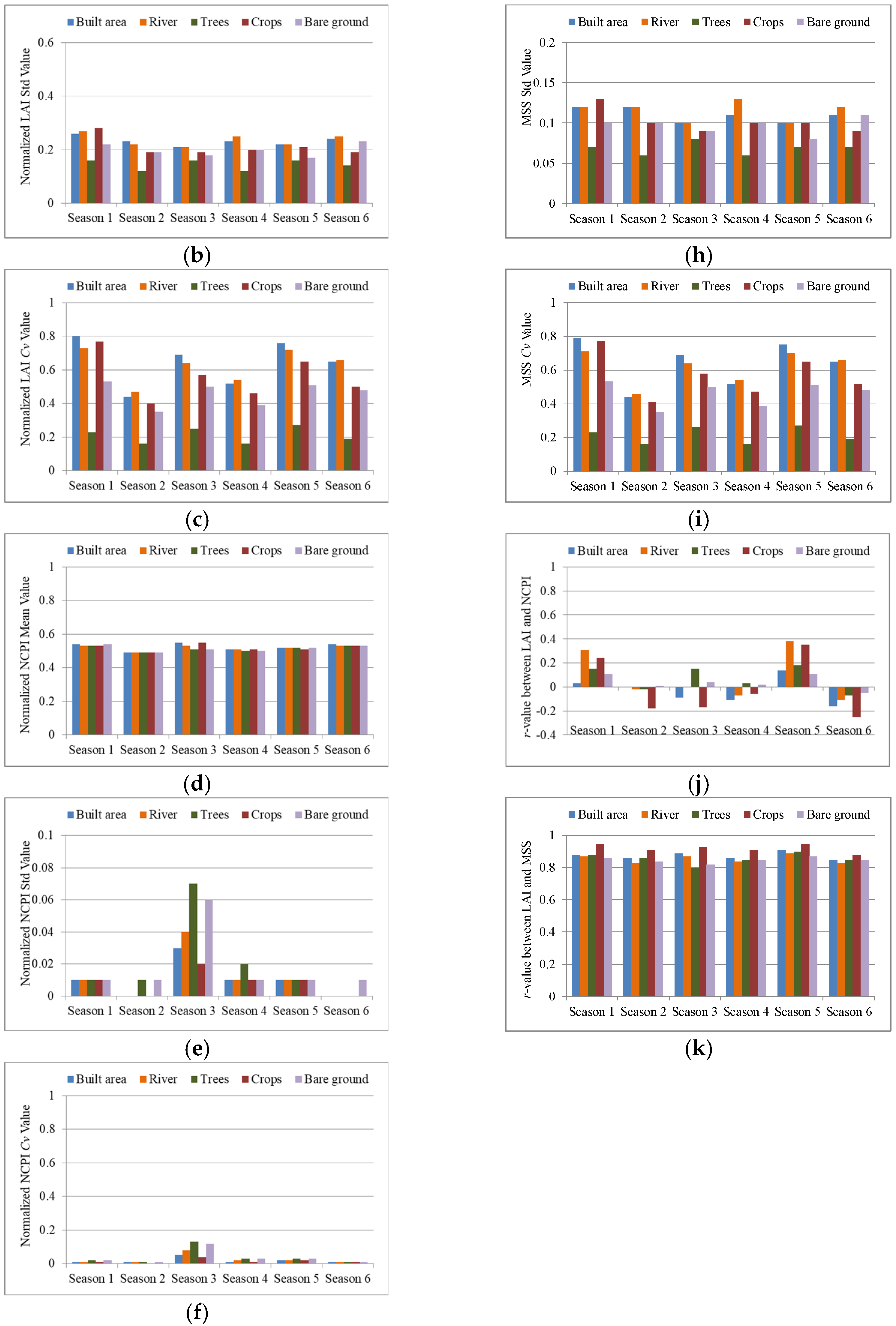
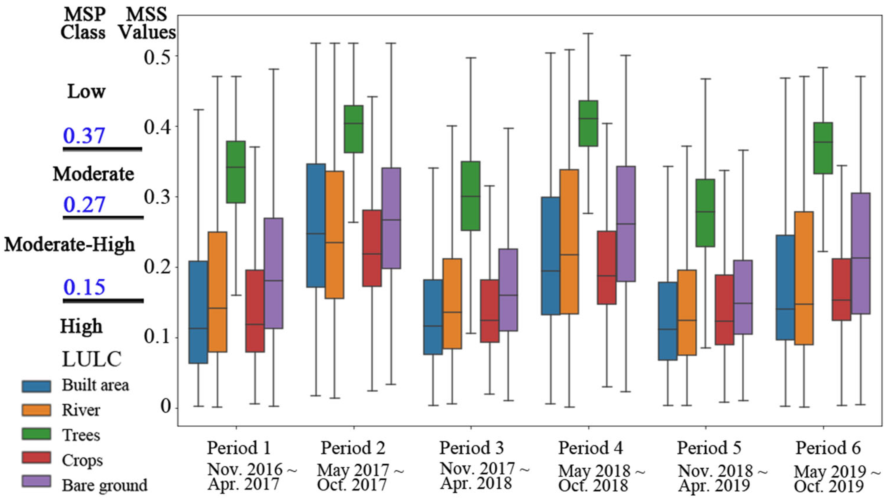
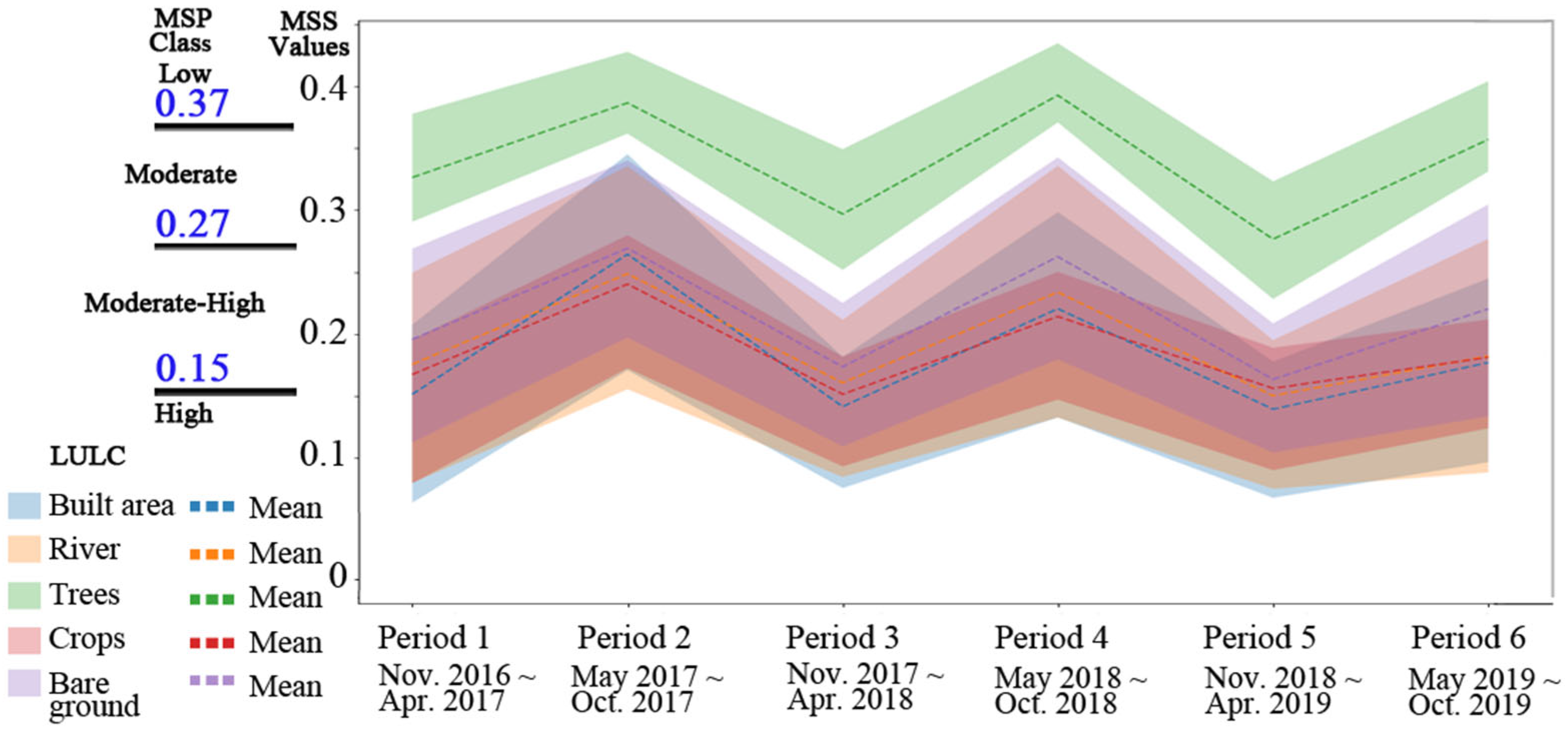
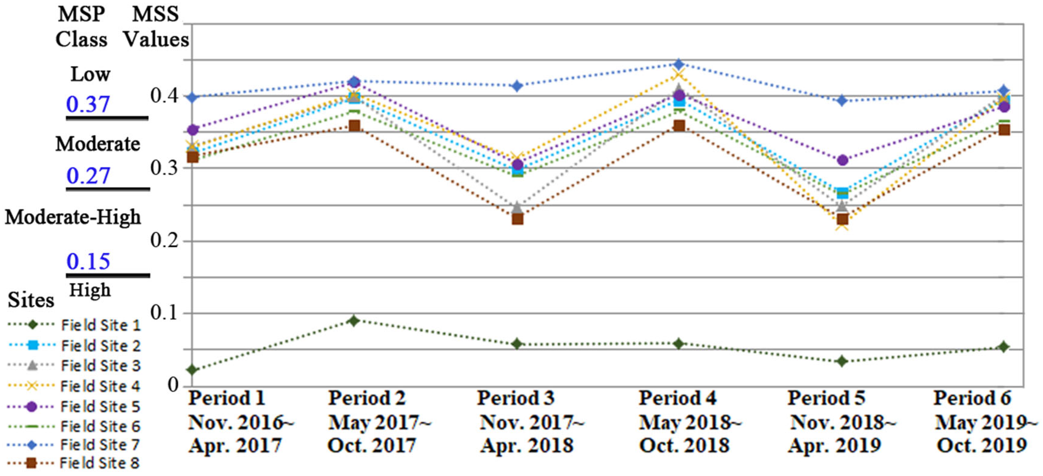
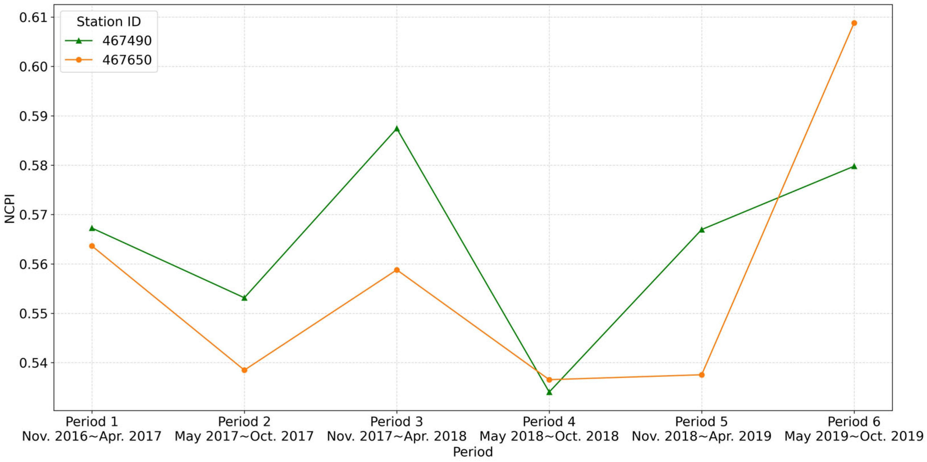
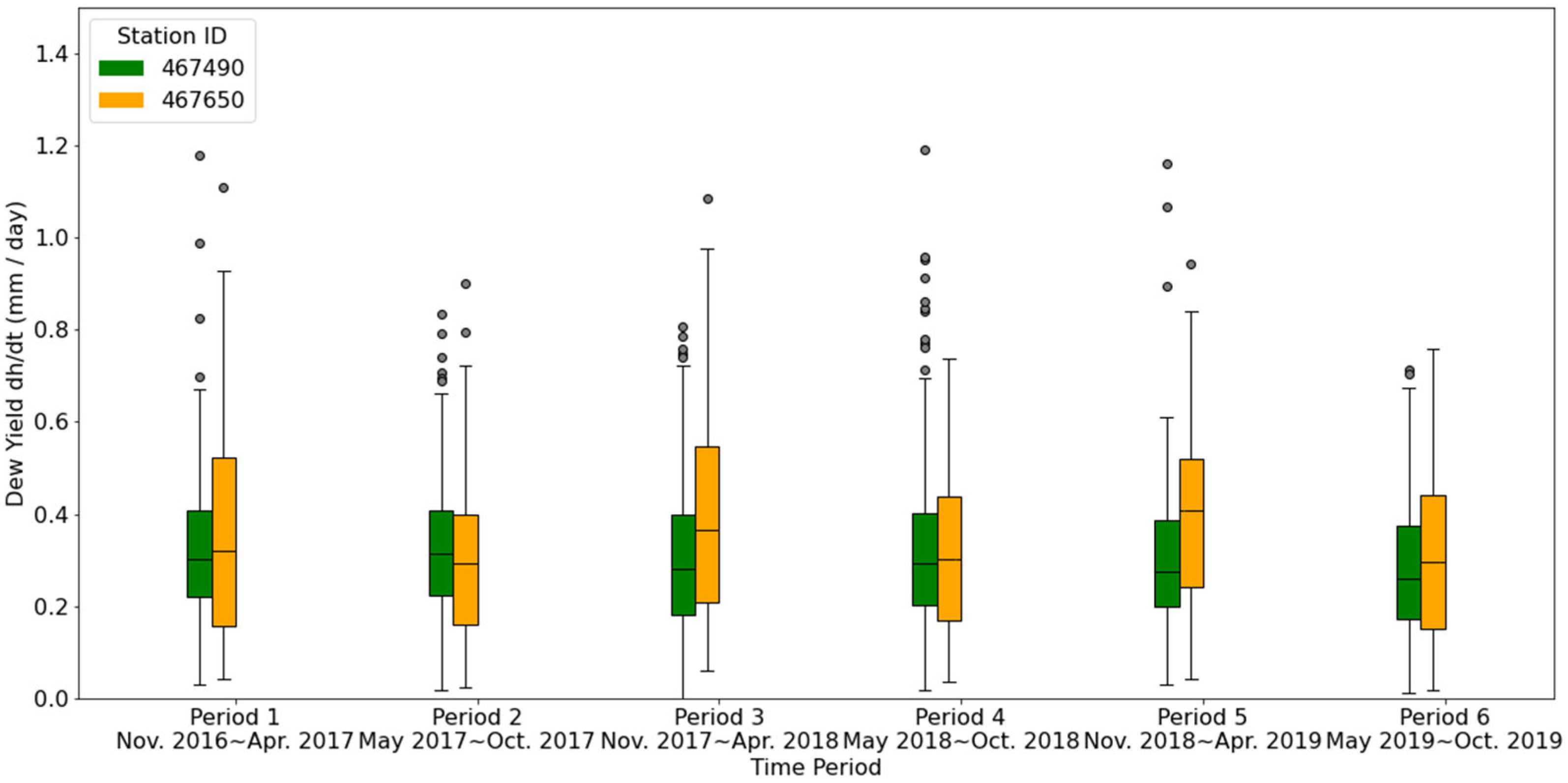

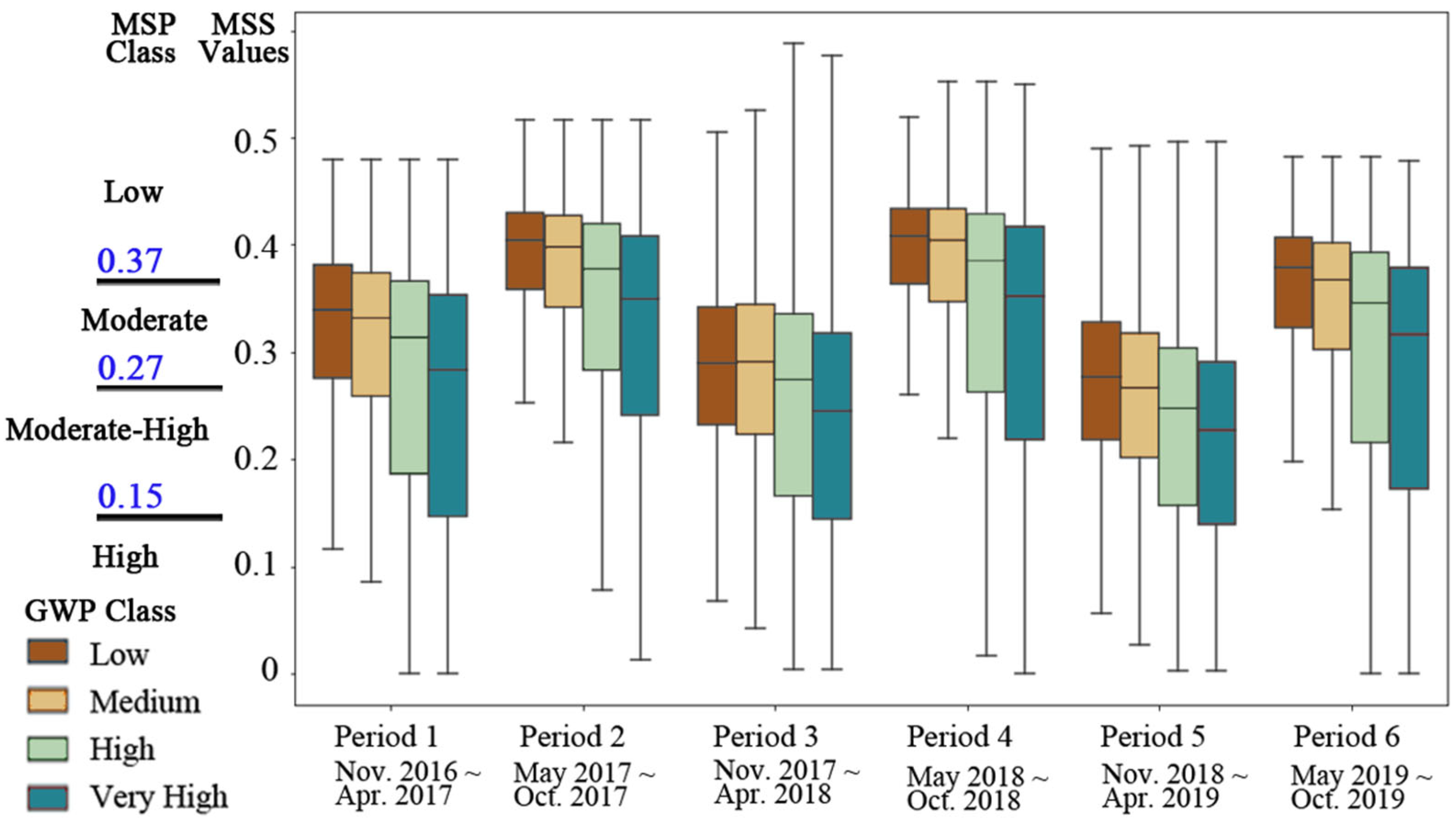
Disclaimer/Publisher’s Note: The statements, opinions and data contained in all publications are solely those of the individual author(s) and contributor(s) and not of MDPI and/or the editor(s). MDPI and/or the editor(s) disclaim responsibility for any injury to people or property resulting from any ideas, methods, instructions or products referred to in the content. |
© 2025 by the authors. Licensee MDPI, Basel, Switzerland. This article is an open access article distributed under the terms and conditions of the Creative Commons Attribution (CC BY) license (https://creativecommons.org/licenses/by/4.0/).