Energy-Efficient Target Area Imaging for UAV-SAR-Based ISAC: Beamforming Design and Trajectory Optimization

Abstract

Integrated Sensing and Communication (ISAC) has been enhanced to serve as a pivotal enabler for next-generation communication systems. In the context of target area detection, a UAV-SAR (Unmanned Aerial Vehicle–Synthetic Aperture Radar) based ISAC system, which shares both physical infrastructure and spectrum, can enhance the utilization of spectrum and hardware resources. However, existing studies on UAV-SAR-based ISAC systems for target imaging remain limited. In this study, we first established an ISAC mechanism to enable SAR imaging and communication. Then, we analyzed the energy consumption model, which includes both UAV propulsion and ISAC energy consumption. To maximize system energy efficiency, we propose an optimization method based on sequential convex optimization with linear state-space approximation. Furthermore, we propose a plan with general constraints, including the initial and final positions, the signal-to-noise ratio (SNR) constraint for SAR imaging, the data transmission rate constraint, and the total power limitation of the UAV. To achieve maximum energy efficiency, we jointly optimized the UAV’s trajectory, velocity, communication beamforming, sensing beamforming, and power allocation. Numerical results demonstrate that compared to existing benchmarks and PSO algorithms, the proposed method significantly improves the energy efficiency of UAV-SAR-based ISAC systems through optimized trajectory design.

1. Introduction

With the rapid improvement of wireless communication, integrated sensing and communication (ISAC) integrates communication and sensing simultaneously, emerging as one of the key technologies for the 6th Generation Mobile Communications System (6G) [1,2]. AS an advanced physical layer technology, ISAC systems share frequency bands and hardware resources to enable both sensing and communication functions. Compared with traditional separate sensing and communication systems, ISAC can enhance both the spectral and energy efficiency. Given its potential, ISAC is expected to play a pivotal role in 6G technology, being widely applied in emergency rescue, regional detection coverage, and other scenarios [3,4,5,6].

Among the diverse platforms for ISAC, Unmanned Aerial Vehicles (UAVs) stand out due to their high mobility, flexible deployment, and strong line-of-sight (LoS) communication capabilities [7]. Traditional UAV platforms often rely on separate communication and sensing devices, increasing the payload burden and limiting operational efficiency. ISAC provides a novel approach to overcoming the limitations of aerial platforms. UAV-enabled ISAC leverages shared communication hardware, effectively reducing payload weight, lowering energy consumption, and enhancing overall UAV performance [8,9]. Compared with traditional airborne systems, UAV-enabled ISAC can simultaneously integrate communication and sensing. Thus, UAV-enabled ISAC has garnered significant attention in both academia and industry [10].

Currently, UAV-ISAC systems still face several challenges. Existing research primarily focuses on enhancing the detection performance of conventional target parameters, including target position, angle of arrival (AoA), and velocity [11,12,13]. However, imaging performance—which is critical for many remote sensing applications—has received significantly less attention.

As an important imaging technology, UAV-SAR is a widely utilized remote sensing technique that enables high-resolution scene awareness in complex environments [14,15,16]. Thus, UAV-SAR based ISAC systems provide a unique opportunity to unify high-resolution radar imaging and real-time communication. They can be widely applied in scenarios requiring both precise environmental perception and efficient data transmission, such as disaster monitoring, battlefield reconnaissance, precision agriculture, and urban surveillance. By integrating sensing and communication capabilities within a single UAV platform, these systems significantly enhance operational efficiency while reducing payload costs.

Despite the promising potential of UAV-enabled ISAC systems, several critical challenges remain unresolved. First, the integration of SAR imaging and real-time communication leads to a large volume of data, which must be handled efficiently under the UAV’s limited energy budget. Second, maximizing energy efficiency is inherently difficult due to the non-convex nature of the optimization problem, which involves coupling between the UAV’s mobility, beamforming, power control, and sensing strategies. Third, practical constraints on imaging quality and communication throughput further complicate the problem formulation and solution design. These challenges necessitate the development of a mathematically rigorous and computationally tractable framework that can jointly optimize multiple coupled variables under realistic UAV operational constraints.

In this paper, we propose a novel UAV-based remote sensing framework that aims to maximize data acquisition while minimizing energy consumption. To this end, we introduce the metric of energy efficiency (EE), defined as the ratio between the total sensing and communication throughput and the UAV’s propulsion energy consumption. Unlike conventional energy optimization methods that primarily focus on reducing UAV energy usage while often overlooking sensing performance, our approach emphasizes a holistic design that jointly considers sensing, communication, and mobility. Specifically, we adopt phased-array SAR in Spotlight mode to enable the high-resolution imaging of target areas, where beamforming is employed to dynamically steer the beam toward the region of interest in real time. The UAV collects sensing data during flight and transmits it back to the base station (BS) simultaneously, making the total data volume consist of both the sensed data and the returned communication data. The UAV initiates its mission from a predefined location, performs SAR imaging along its trajectory, and completes the operation upon reaching the final destination. To maximize EE, we jointly optimize the UAV’s trajectory, velocity, beamforming pattern, and the allocation of sensing and communication power. A sequential convex optimization method based on linear state-space approximation is proposed to obtain a locally optimal solution. Simulation results validate the effectiveness of the proposed framework, demonstrating significant improvements in power allocation, flight trajectory, and overall energy efficiency.

The main contributions of this work are summarized as follows:

• We formulate a novel energy-efficiency maximization problem for a UAV-SAR-based integrated sensing and communication (ISAC) system. The problem jointly considers SAR imaging and sensing data transmission under realistic constraints on imaging quality and communication rate. The total data volume comprises both received echo data and transmitted sensing data. The resulting optimization problem is a highly non-convex fractional program with a non-concave numerator and a non-convex denominator. To address this challenge, we transform the original formulation into a tractable form with a concave numerator and a convex denominator, enabling the use of fractional programming techniques.
• To efficiently solve the transformed problem, we propose a sequential convex optimization framework based on linear state-space approximation. The proposed algorithm jointly optimizes the UAV’s flight trajectory, velocity profile, beamforming strategy, and power allocation. Moreover, non-convex constraints are approximated through convex reformulations, ensuring that each iteration can be solved efficiently with theoretical convergence guarantees.
• Comprehensive simulation results demonstrate the effectiveness of the proposed approach. Compared with baseline schemes, the proposed method significantly enhances the energy efficiency of the UAV-enabled ISAC system. These findings underscore the importance of the joint optimization of mobility and communication resources and provide valuable insights for the practical deployment of ISAC systems in UAV-SAR applications.

The remainder of this paper is organized as follows. Section 2 reviews the related works including the UAV-enabled ISAC systems, UAV-SAR imaging, and energy-efficient UAV operations. Section 3 introduces the system model, including the SAR imaging model, UAV communication model, energy consumption model, and system energy efficiency formulation. Section 4 details the proposed solution approach. Section 5 presents simulation results to evaluate the performance of the proposed algorithm. Finally, Section 6 concludes this paper.

2. Related Works

In this section, we provide a brief review of recent advances in UAV-enabled ISAC systems, UAV-SAR imaging, and energy-efficient UAV operations.

2.1. UAV-Enabled ISAC Systems

UAV-enabled ISAC systems offer high mobility, flexibility, and controllability and can establish strong line-of-sight (LoS) air-to-ground communication links. Beamforming techniques are widely adopted to enhance the performance of ISAC systems by improving signal quality and spatial resolution. As a signal processing technology, beamforming can enhance the signal and suppress the interference in a specific direction by weighting the signals of multiple antennas to realize directional signal transmission or reception. Jointly designing the resource allocation strategy, beamforming scheme, and UAV trajectory to fully exploit the potential of UAV-enabled ISAC systems remains a highly promising yet inherently challenging problem.

Various beamforming design methods have been proposed, enabling UAV-enabled ISAC to provide high-quality ISAC services. In [11], the authors considered the challenges of wireless resource wastage and low system resource utilization in UAV-based multi-target sensing and communication scenarios. They proposed a novel Adaptive ISAC (AISAC) mechanism, which optimizes communication and sensing beamforming as well as UAV trajectory to maximize the average system throughput. In [12], for an ISAC system with simultaneous sensing and communication, the authors designed the transmit beamforming to maximize the detection performance under the condition of satisfying the SNR of the communication users. In [13], in order to enhance the communication and sensing coverage and improve the comprehensive gain of communication and sensing, the authors jointly optimized the UAV trajectory and beamforming design to improve the performance of the UAV-enabled ISAC system. Imaging performance for target detection enables one to acquire more detailed target information, which is not achievable with conventional radar detection methods.

2.2. UAV-SAR Imaging

UAV-SAR, as an important imaging technology, can not only offer large-area observation and high-resolution imaging capabilities but also obtain targets information as conventional radars, remaining unaffected by lighting and weather conditions. The commonly used UAV-SAR modes mainly include StripMap mode and Spotlight mode. The StripMap mode of SAR is mainly used to scan and image the large area. In StripMap mode, the beam direction remains fixed while the platform moves, causing the beam to sweep uniformly across the ground and generate continuous strip images. This mode provides wide-area coverage but lacks detailed imaging of specific target regions, making it suitable for large-scale imaging [17]. However, in Spotlight mode, the antenna beam tracks a target area within a certain range, increasing the observation time for that region and enabling the acquisition of high-resolution images [18]. By synthesizing multiple beam echoes from the target area, a high-resolution image can be obtained. While Spotlight mode offers high observation efficiency, its coverage area is relatively small.

The current research on UAV-SAR target area imaging mainly includes the following research [19,20]. In [19], the authors proposed a BS-UAV bistatic SAR platform for UAV-enabled ISAC for target area detection, where the BS (Base Station) transmits signals at a fixed angle within the target area. A single rotary-wing UAV receives both the communication signals from the BS and the target-reflected signals to obtain imaging information. By optimizing the UAV’s flight trajectory, they effectively reduced UAV flight energy consumption. In [20], the authors investigated the problem of maximizing SAR imaging coverage for UAVs scanning a square area. They proposed a low-complexity suboptimal algorithm based on successive convex approximation. By jointly optimizing UAV resources and three-dimensional (3D) trajectory while ensuring imaging quality and communication reliability with the BS, they enhanced SAR radar coverage of the target area. UAV-SAR-based ISAC enables simultaneous target area imaging and communication, enhancing system efficiency, adaptability, and intelligence. This technology holds significant research value and demonstrates immense application potential across military, civil, and emergency response domains. Although UAV-SAR can provide high-resolution remote sensing images, considering the limited energy budget of UAVs in practical applications, maximizing the amount of information acquired per unit of energy consumption has emerged as a critical challenge in system design [21].

2.3. Energy-Efficient UAVs

Current research on UAV energy efficiency primarily focuses on communication scenarios [22,23,24]. In [22], the authors investigated the energy efficiency problem in a fixed-wing UAV-to-BS direct communication scenario. By jointly optimizing the UAV’s flight radius, trajectory, acceleration, and velocity using a sequential convex optimization approach, they achieved maximum energy efficiency for the UAV. In [23], the authors optimized the 3D trajectory of a fixed-wing UAV and adopted the convex difference function and continuous convex approximation method to maximize the communication efficiency of the UAV. In [24], the authors investigated the energy efficiency problem in a scenario where a fixed-wing UAV, serving as a relay node, forwards received information from the BS to ground nodes (GNs) in real time. By jointly optimizing the UAV’s trajectory, acceleration, and velocity while incorporating an information causality constraint, they employed an alternating iterative optimization approach to enhance UAV energy efficiency. In [25], the authors investigated the energy consumption minimization problem for a rotary-wing UAV collecting data from a ground wireless sensor network (WSN). By optimizing the node wake-up mechanism and UAV trajectory using a successive convex approximation-based joint optimization approach, they achieved a trade-off between the energy consumption of the UAV and SNs. However, there are few studies on the target sensing energy efficiency of UAV-enabled ISAC. Due to the limited energy consumption of UAVs, UAV-enabled ISAC uses less energy to obtain more target sensing data and transmit it back to the BS. Considering the large volume of real-time sensing and communication data in UAV-SAR-based ISAC, optimizing energy efficiency becomes even more critical in system design. Therefore, we investigated the problem of maximizing the energy efficiency of UAV-SAR-based ISAC for target area imaging.

This paper proposes an energy-efficient UAV-SAR-based ISAC sensing framework that integrates Spotlight-mode beamforming for high-resolution imaging and real-time data transmission. Joint optimization of trajectory, velocity, beamforming, and power control was performed to maximize energy efficiency. A sequential convex optimization method was developed, and the simulation results validate the effectiveness of the proposed approach.

3. System Model

In this section, a UAV-ISAC target area sensing and communication model is described, including a UAV-SAR imaging model, a communication model, and a UAV energy consumption model. Then, a joint optimization problem is formulated for UAV energy efficiency, considering trajectory, sensing and communication beamforming parameters, and flight velocity. The main notations are listed in

Table 1. Notation table.

Notation	Physical Meaning
$r^{\left(m\right)}$	Radius of detection area
H	UAV flight altitude
$PRF$	Pulse repetition frequency
$Br$	Radar bandwidth
$SN{R}_{min}$	SAR imaging SNR threshold
$V_{Max}$	Maximum UAV speed
${\tau }_p$	Radar pulse duration
B	Transmission bandwidth
$\lambda$	Wavelength
$P_0$	Blade profile power
$P_1$	Rotor-induced power
$U_{tip}$	Tip speed
$v_0$	Rotor velocity
S	Rotor solidity
A	Disc area
$P_{max}$	UAV power upper limit
${\theta }_d$	Radar elevation range
$\mu$	Subslot allocation coefficient
${\mathbf{a}}_{\mathbf{T}}$	Transmit steering vector of sensing
$\mathbf{f}$	Beamforming vector of sensing
$R^{dr}$	Sensing data rate
R	Data rate of UAV
${\mathrm{SNR}}^{\left(rad\right)}$	UAV-SAR imaging SNR
$\gamma$	Communication SNR
$\mathbf{H}$	Communication channel matrix
$EE$	Energy-efficiency of UAV
E	Energy consumption of UAV

.

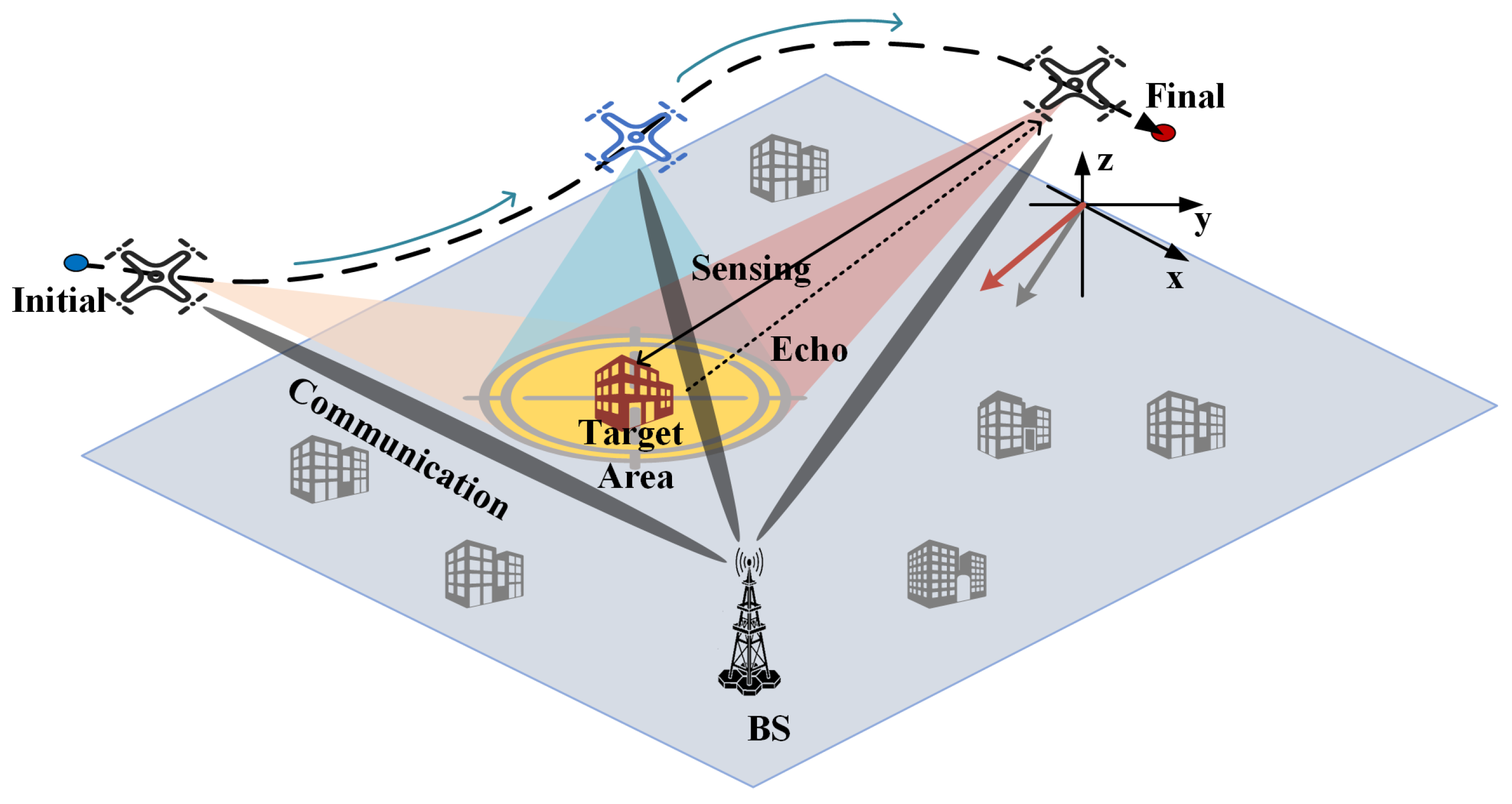
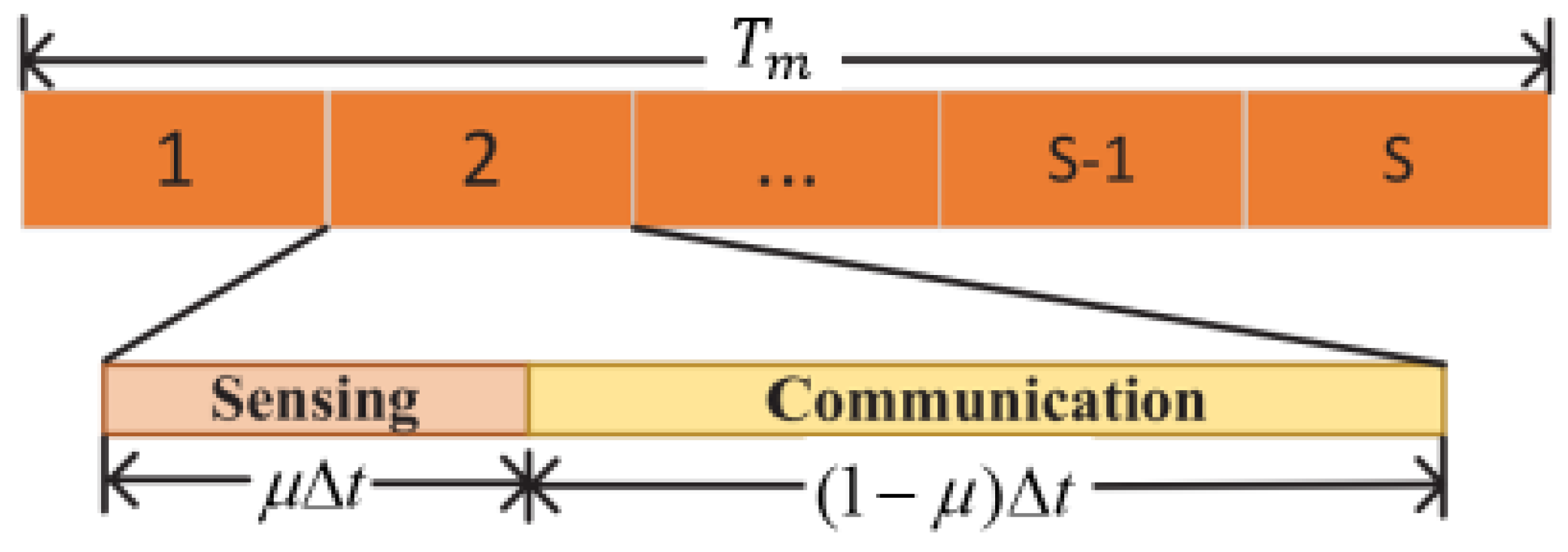
Consider a single rotary-wing UAV equipped with an $m\times m$ array antenna, which departs from the initial position to perform SAR imaging of a single target area while transmitting the sensing data to the BS in real time, as shown in Figure 1. The UAV continues this process until it reaches the final position, completing the target area sensing. The UAV-SAR uses Spotlight mode to sense the target area and beamforming to control the beam direction of perception and communication. During the communication and sensing process, it divides each time slot into two sub-slots, with sub-slot $\mu \Delta t$ dedicated to sensing and sub-slot $(1-\mu )\Delta t$ used for communication, as shown in Figure 2. The position at time slot n of the UAV is $\mathbf{q}\left[n\right]={[x_n,y_n]}^T\in {\mathrm{R}}^{2\times 1}$, $n\in [0,N]$. The UAV flies at a constant altitude $\mathrm{H}$, and the inital and final positions are denoted as $\mathbf{q}\left[0\right]$ and $\mathbf{q}\left[N\right]$, respectively, which are within the range of the UAV detection area. The center coordinate of the detected target area is defined as $[0,0]$.

3.1. Radar Sensing and Imaging Model

In the first subslot of time slot n, the SAR signal transmitted by the UAV is denoted as s. ${\theta }_d$ and ${\phi }_d$ denote the elevation and azimuth angles between the UAV and the target area, respectively. The steering vector matrices are between the transmitter and defined as ${\mathbf{a}}_{\mathbf{T}}\in {\mathrm{C}}^{1\times m^2}$, transmit steering vector ${\mathbf{a}}_{\mathbf{T}}=[a_{11},\dots ,a_{1m},a_{21},\dots ,a_{2m},\dots ,a_{m1},\dots ,a_{mm}]$, and $a_{jk}=e^{j\pi [(j-1)sin{\theta }_{d}cos{\phi }_d+(k-1)sin{\theta }_{d}sin{\phi }_d]}$. In the UAV-SAR Spotlight model, beamforming is used to control the direction of the transmitted radar signals, which is represented by $\mathbf{f}\in {\mathrm{f}}^{m^2\times 1}$. Therefore, the echo signal $\mathbf{r}$ received by the UAV from the target area can be expressed as

$$\begin{array}{c}\hfill \mathbf{r}=\alpha {\mathbf{a}}_T{\mathbf{a}}_T^H\mathbf{f}s+\mathbf{n},\end{array}$$

(1)

where $\alpha$ represents the reflection coefficient, s denotes the transmitted sensing symbol with a unit energy constraint, and $\mathbf{n}$ is the stacked vector of zero-mean additive white Gaussian noise (AWGN) at the receiving antenna input. During the target area sensing and imaging process, the sensing signal transmission power is $P^{SAR}={∥\mathbf{f}∥}^2$. UAV-SAR uses Spotlight mode to sense and image the target area, and the sensing data rate $R^{dr}$ can be expressed as

$$\begin{array}{c}\hfill R^{dr}\left[n\right]=B_r({\displaystyle \frac{2H\Omega \left[n\right]}{c}}+{\tau }_p)PRF[\mathrm{bit}/\mathrm{s}],\end{array}$$

(2)

where $B_r$ is the radar bandwidth, ${\tau }_p$ is the radar pulse duration, c is the speed of light, $PRF$ is the radar pulse repetition frequency, and $\Omega \left[n\right]$ is the distance difference between UAV detection far point and near point and the ratio of UAV flight height in time slot n [26]. $\Omega \left[n\right]$ can be written as

$$\begin{array}{cc}\hfill \Omega \left[n\right]=& {\displaystyle \frac{1}{cos\left({\theta }_2\left[n\right]\right)}}-{\displaystyle \frac{1}{cos\left({\theta }_1\left[n\right]\right)}}\hfill \\ \hfill =& {\displaystyle \frac{cos\left({\theta }_1\left[n\right]\right)-cos\left({\theta }_2\left[n\right]\right)}{cos\left({\theta }_1\left[n\right]\right)cos\left({\theta }_2\left[n\right]\right)}},\hfill \end{array}$$

(3)

where ${\theta }_1\left[n\right]={\theta }_d\left[n\right]-{\Theta }_{3\mathrm{dB}}/\phantom{{\Theta }_{3\mathrm{dB}}2}2$ and ${\theta }_2\left[n\right]={\theta }_d\left[n\right]+{\Theta }_{3\mathrm{dB}}/\phantom{{\Theta }_{3\mathrm{dB}}2}2$. ${\Theta }_{3\mathrm{dB}}$ is the $3\mathrm{dB}$ beamwidth of the radar antenna and ${\theta }_d$ is the radar depression Angle, denoted as ${\theta }_d\left[t\right]=arctan∥\mathbf{q}\left[n\right]∥/\phantom{∥\mathbf{q}\left[n\right]∥H}H$.

UAV-SAR imaging SNR can be expressed as

$$\begin{array}{c}\hfill {\mathrm{SNR}}^{\left(\mathrm{rad}\right)}\left[n\right]={\displaystyle \frac{{∥\mathbf{f}∥}^2{\lambda }^3{G}_t{G}_r{\sigma }_{0}c·{\tau }_p·PRF·{cos}^2{\theta }_d\left[n\right]}{{\left(4\pi \right)}^4{H}^{3}k·T_o·NF·B_r{L}_{\mathrm{tot}}v\left[n\right]}},\end{array}$$

(4)

where $\lambda$ represents the detection wavelength and $G_t$ and $G_r$ are the radar antenna transmission and reception gains, respectively [27]. The radar backscatter coefficient is denoted as ${\sigma }_0$. The Boltzmann constant is denoted as k. $T_o$ is the equivalent noise factor. $NF$ is the system noise figure and the overall loss factor is denoted as $L_{\mathrm{tot}}$.

3.2. Communication Model

Considering that the communication process of the UAV forwarded to the BS is similar to the above process, ${\eta }_n$ and ${\tau }_n$ are used to represent the elevation and azimuth angles between the UAV and the BS, respectively. The communication channel variation between the UAV and BS is induced by the change in relative angles under constant-altitude flight. Given the constant flight altitude, the variation of the relative angle is attributed to the changes in the UAV’s planar (horizontal) position. The sensing data signal y received by the BS can be expressed as $y={\mathbf{u}}^H(\mathbf{Hw}x+\mathbf{n})$. The communication SNR is

$$\begin{array}{cc}\hfill \gamma =& {\displaystyle \frac{E\left[x^H{\mathbf{w}}^H{\mathbf{H}}^H{\mathbf{u}}^H\mathbf{uHw}x\right]}{E\left[{\mathbf{n}}^{\mathbf{H}}{\mathbf{u}}^H\mathbf{u}\mathbf{n}\right]}}\hfill \\ \hfill =& {\displaystyle \frac{E\left[{\mathbf{w}}^H{\mathbf{H}}^H\mathbf{Hw}\right]}{{\sigma }^2\mathbf{u}{\mathbf{u}}^H}},\hfill \end{array}$$

(5)

where x is the data sent by the UAV and y is the data received by the BS. The beamforming vectors at the UAV transmitter and BS receiver can be denoted as $\mathbf{w}\in {\mathrm{C}}^{m^2\times 1}$ and $\mathbf{u}\in {\mathrm{C}}^{m^2\times 1}$, respectively. $\mathbf{H}$ is the communication channel matrix. The receiving rate at the BS can be expressed as

$$\begin{array}{c}\hfill R=B^{com}{log}_2(1+\gamma ),\end{array}$$

(6)

where $B^{com}$ is the communication bandwidth and the transmit power is $P^{com}={∥\mathbf{w}∥}^2$.

3.3. UAV Energy Consumption Model

The moving power model for a rotary-wing UAV can be modeled as

$$\begin{array}{c}\hfill P^{fly}\left(v\right)=P_0\left(1+{\displaystyle \frac{3v^2}{U_{\mathrm{tip}}^2}}\right)+P_1{\left(\sqrt{1+{\displaystyle \frac{v^4}{4v_0^4}}}-{\displaystyle \frac{v^2}{2v_0^2}}\right)}^{1/2}+C_0{v}^3,\end{array}$$

(7)

where $C_0=1/\phantom{12}2d_0\rho sA$, $d_0$ is the UAV fuselage drag ratio, s is the UAV rotor solidity, $\rho$ is the air density coefficient in the UAV’s flight environment, and A is the rotor disk area of the UAV. $P_0$ and $P_1$ represent the blade profile power and induced power of the UAV in a hovering state, respectively. v denotes the UAV’s flight velocity. $U_{tip}$ denotes the tip speed of the rotor blades and $v_0$ represents the average rotor induced velocity in the hovering state [28].

The total power consumption of the UAV includes both propulsion power and ISAC power. Therefore, the total energy consumption $E\left\{\mathbf{q}\right[n\left]\right\}$ of the UAV over the total time slots N is given by

$$\begin{array}{cc}\hfill E\left\{\mathbf{q}\right[n\left]\right\}=& \sum _{n=1}^N[P_0\left(1+{\displaystyle \frac{3v{\left[n\right]}^2}{U_{\mathrm{tip}}^2}}\right)+P_1{\left(\sqrt{1+{\displaystyle \frac{v{\left[n\right]}^4}{4v_0^4}}}-{\displaystyle \frac{v{\left[n\right]}^2}{2v_0^2}}\right)}^{1/2}\hfill \\ \hfill & +C_{0}v{\left[n\right]}^3+(1-\mu )·{∥\mathbf{w}\left[n\right]∥}^2+\mu ·{∥\mathrm{f}\left[n\right]∥}^2]·\Delta t,\hfill \end{array}$$

(8)

with $v\left[n\right]=∥\mathbf{q}\left[n\right]-\mathbf{q}[n-1]∥/\phantom{∥\mathbf{q}\left[n\right]-\mathbf{q}[n-1]∥\Delta t}\Delta t$ denoting the relationship between drone flight speed and trajectory, which represents the velocity of the UAV in each time slot.

The total data volume $R\left\{\mathbf{q}\right[n\left]\right\}$ of the UAV over N time slots consists of both sensing and communication data. Therefore, the total data volume is given by:

$$\begin{array}{c}\hfill R\left\{\mathbf{q}\left[n\right]\right\}=\sum _{n=1}^N[B_r({\displaystyle \frac{2H\Omega \left[n\right]}{c}}+{\tau }_p)PRF+B^{com}{log}_2(1+\gamma )]\Delta t,\end{array}$$

(9)

The energy efficiency $EE\left\{\mathbf{q}\right[n\left]\right\}$ of the UAV at time slot n is given by

$$\begin{array}{c}\hfill EE\left\{\mathbf{q}\left[n\right]\right\}={\displaystyle \frac{R\left\{\mathbf{q}\right[n\left]\right\}}{E\left\{\mathbf{q}\right[n\left]\right\}}},\end{array}$$

(10)

To maximize the energy efficiency of the UAV, the problem (P0) can be formulated as

$$\begin{array}{cc}\hfill \left(\mathrm{P}0\right):& \underset{{\displaystyle \genfrac{}{}{0pt}{}{\left\{\mathbf{q}\right[n],v[n],\mathbf{w}[n],\hfill }{\mathbf{f}\left[n\right],{\theta }_d\left[n\right]\}\hfill }}}{max}{\displaystyle \frac{{\displaystyle \sum _{n=1}^N}R\left\{\mathbf{q}\right[n\left]\right\}}{{\displaystyle \sum _{n=1}^N}E\left\{\mathbf{q}\right[n\left]\right\}}}\hfill \\ \hfill s.t.& \\ \hfill & C1:\mathbf{q}\left[0\right]=[x_{ini},y_{ini}],\hfill \\ \hfill & C2:\mathbf{q}\left[N\right]=[x_{fin},y_{fin}],\hfill \\ \hfill & C3:0\le v\left[n\right]\le v_{max},\hfill \\ \hfill & C4:(1-\mu )R^{com}\ge \mu R^{dr},\hfill \\ \hfill & C5:0\le {∥\mathbf{w}\left[n\right]∥}^2+P^{fly}\left[n\right]\le P_{max},\hfill \\ \hfill & C6:0\le {∥\mathrm{f}\left[n\right]∥}^2+P^{fly}\left[n\right]\le P_{max},\hfill \\ \hfill & C7:{\mathrm{SNR}}^{\left(\mathrm{rad}\right)}\left[n\right]\ge {\mathrm{SNR}}_{min},\hfill \\ \hfill & C8:0^{\circ }\le {\theta }_d\left[n\right]\le {60}^{\circ },\hfill \end{array}$$

(11)

In practical scenarios, the UAV must satisfy multiple constraints $C1$–$C8$. Specifically, $C1$ and $C2$ define the initial and final positions of the UAV. The initial and final positions meet the minimum SNR threshold of perception according to the above. Constraint $C3$ imposes a velocity limit of the UAV, while $C4$ ensures the required sensing and communication data rate, where compliance with $C3$ is necessary to guarantee the successful transmission of the sensed target area image data to the BS. Constraints $C5$ and $C6$ regulate the UAV’s power consumption. Constraint $C7$ enforces a sensing threshold, ensuring that the UAV can successfully detect the target when the SNR of the SAR image exceeds a predefined threshold ${\mathrm{SNR}}_{\min }$. Finally, constraint $C8$ restricts the UAV-SAR detection angle.

4. Proposed Approach

In this section, we first transform the original problem. Then, we separately handle the numerator and denominator, reformulating the original problem into a new optimization problem aimed at maximizing a system function characterized by a concave numerator and a convex denominator. Finally, we convexify the non-convex constraints and solve the resulting problem.

4.1. Concave Transformation of the Numerator

This subsection first reformulates the problem (P0) and then transforms the numerator of the new function into a concave form. Furthermore, a lower bound of the resulting function is derived and rigorously proven.

Since problem (P0) is a non-convex problem, it is difficult to solve directly. To overcome this difficulty, we propose employing a convex approximation method. Considering the UAV sensing and communicating in real time, the volume of forwarded data must be at least equal to the generated sensing data, a condition explicitly enforced by constraint $C4$.

$$\begin{array}{c}\hfill R\left\{\mathbf{q}\left[n\right]\right\}\ge 2\sum _{n=1}^N\mu B_r({\displaystyle \frac{2H\Omega \left[\mathbf{q}\right[n\left]\right]}{c}}+{\tau }_p)PRF,\end{array}$$

(12)

Thus,

$$\begin{array}{c}\hfill {\displaystyle \frac{{\displaystyle \sum _{n=1}^N}R\left\{\mathbf{q}\right[n\left]\right\}}{{\displaystyle \sum _{n=1}^N}E\left\{\mathbf{q}\right[n\left]\right\}}}\ge {\displaystyle \frac{2{\displaystyle \sum _{n=1}^N}\left[\mu B_r(\frac{2H\Omega \left[\mathbf{q}\right[n\left]\right]}{c}+{\tau }_p)PRF\right]\Delta t}{{\displaystyle \sum _{n=1}^N}E\left\{\mathbf{q}\right[n\left]\right\}}},\end{array}$$

(13)

The original problem (P0) can be approximated and reformulated as the following new problem (P1):

$$\begin{array}{cc}\hfill \left(\mathrm{P}1\right):& \underset{{\displaystyle \genfrac{}{}{0pt}{}{\left\{\mathbf{q}\right[n],v[n],\mathbf{w}[n],\hfill }{\mathrm{f}\left[n\right],{\theta }_d\left[n\right]\}\hfill }}}{max}{\displaystyle \frac{2{\displaystyle \sum _{n=1}^N}\left[\mu B_r(\frac{2H\Omega \left[\mathbf{q}\right[n\left]\right]}{c}+{\tau }_p)PRF\right]\Delta t}{{\displaystyle \sum _{n=1}^N}E\left\{\mathbf{q}\right[n\left]\right\}}}\hfill \\ \hfill s.t.& \\ \hfill & C1-C8,\hfill \end{array}$$

(14)

Problem (P1) involves a fractional objective function characterized by a non-concave numerator and a non-convex denominator, thus making it neither convex nor quasi-convex. Consequently, standard convex optimization methods cannot be directly utilized to obtain a solution. Nevertheless, by leveraging sequential convex optimization (SCO) techniques, an efficient solution that satisfies the Karush–Kuhn–Tucker (KKT) conditions can be derived, resulting in a locally optimal solution. To accomplish this, we first handle the non-concavity of the numerator in the objective function. Specifically, for any local point $\left\{{\mathbf{q}}_j\left[n\right]\right\}$ obtained during the jth iteration, we define the following approximated function:

$$\begin{array}{cc}\hfill {\overline{R}}_{lb}\left\{\mathbf{q}\left[n\right]\right\}=& C_1·{\tau }_{p}N+{\displaystyle \frac{C_{1}H}{c}}\sum _{n=1}^N{\alpha }_j\left[n\right]+{\beta }_j{\left[n\right]}^T(\mathbf{q}\left[n\right]-{\mathbf{q}}_j\left[n\right])\hfill \\ \hfill =& C_1·{\tau }_{p}N+{\displaystyle \frac{C_{1}H}{c}}\sum _{n=1}^N{\overline{\Omega }}_{lb}\left(\mathbf{q}\left[n\right]\right),\hfill \end{array}$$

(15)

where $C_1=4B_r·PRF$. The function ${\Omega }_{lb}\left(\mathbf{q}\left[n\right]\right)$ is concave with respect to $\left\{\mathbf{q}\left[n\right]\right\}$, thereby ensuring that ${\overline{R}}_{lb}\left\{\mathbf{q}\left[n\right]\right\}$ is also concave with respect to $\left\{\mathbf{q}\left[n\right]\right\}$.

$$\begin{array}{c}\hfill \Omega \left[\mathrm{q}\left[n\right]\right]=\left({\displaystyle \frac{1}{cos\left(arctan\frac{\parallel \mathbf{q}\left[n\right]\parallel }{H}+\frac{{\Theta }_{3\mathrm{dB}}}{2}\right)}}-{\displaystyle \frac{1}{cos\left(arctan\frac{\parallel \mathbf{q}\left[n\right]\parallel }{H}-\frac{{\Theta }_{3\mathrm{dB}}}{2}\right)}}\right),\end{array}$$

(16)

$$\begin{array}{c}\hfill {\Omega }_{lb}\left(\mathrm{q}\left[n\right]\right)={\alpha }_j\left[n\right]+{\beta }_j{\left[n\right]}^T(\mathbf{q}\left[n\right]-{\mathbf{q}}_j\left[n\right]),\end{array}$$

(17)

Consequently, for any given point $\left\{\mathbf{q}\left[n\right]\right\}$, the following inequality holds:

$$\begin{array}{cc}\hfill \sum _{n=1}^N\Omega \left[\mathbf{q}\right[n\left]\right]\ge & \sum _{n=1}^N{\overline{\Omega }}_{lb}\left[\mathbf{q}\left[n\right]\right]\hfill \\ \hfill =& \sum _{n=1}^N{\alpha }_j\left[n\right]+{\beta }_j{\left[n\right]}^T(\mathbf{q}\left[n\right]-{\mathbf{q}}_j\left[n\right]),\hfill \end{array}$$

(18)

where ${\alpha }_j\left[n\right]$ and ${\beta }_j\left[n\right]$ can be written as

$$\begin{array}{c}\hfill {\alpha }_j\left[n\right]=\sum _{n=1}^N({\displaystyle \frac{1}{cos(arctan\frac{∥\mathbf{q}\left[n\right]∥}{H}+{\Theta }_{3\mathrm{dB}}/\phantom{{\Theta }_{3\mathrm{dB}}2}2)}}-{\displaystyle \frac{1}{cos(arctan\frac{∥\mathbf{q}\left[n\right]∥}{H}-{\Theta }_{3\mathrm{dB}}/\phantom{{\Theta }_{3\mathrm{dB}}2}2)}}),\end{array}$$

(19)

$$\begin{array}{cc}\hfill {\beta }_j{\left[n\right]}^T=& {\displaystyle \frac{{\mathbf{q}}_j\left[n\right]/\phantom{{\mathbf{q}}_j\left[n\right]∥{\mathbf{q}}_j\left[n\right]∥}∥{\mathbf{q}}_j\left[n\right]∥}{H\left(1+{∥{\mathbf{q}}_j\left[n\right]∥}^2/\phantom{{∥{\mathbf{q}}_j\left[n\right]∥}^2{H}^2}{H}^2\right)}}\left({\displaystyle \frac{sin\left(arctan∥{\mathbf{q}}_j\left[n\right]∥/\phantom{∥{\mathbf{q}}_j\left[n\right]∥H}H-{\Theta }_{3\mathrm{dB}}/\phantom{{\Theta }_{3\mathrm{dB}}2}2\right)}{{cos}^2\left(arctan∥{\mathbf{q}}_j\left[n\right]∥/\phantom{∥{\mathbf{q}}_j\left[n\right]∥H}H-{\Theta }_{3\mathrm{dB}}/\phantom{{\Theta }_{3\mathrm{dB}}2}2\right)}}\right.\hfill \\ \hfill & \left.-{\displaystyle \frac{sin\left(arctan∥{\mathbf{q}}_j\left[n\right]∥/\phantom{∥{\mathbf{q}}_j\left[n\right]∥H}H+{\Theta }_{3\mathrm{dB}}/\phantom{{\Theta }_{3\mathrm{dB}}2}2\right)}{{cos}^2\left(arctan∥{\mathbf{q}}_j\left[n\right]∥/\phantom{∥{\mathbf{q}}_j\left[n\right]∥H}H+{\Theta }_{3\mathrm{dB}}/\phantom{{\Theta }_{3\mathrm{dB}}2}2\right)}}\right),\hfill \end{array}$$

(20)

Theorem 1.

For any given local point $\left\{{\mathbf{q}}_j\left[n\right]\right\}$, we have (18). When $\mathbf{q}\left[n\right]={\mathbf{q}}_j\left[n\right]$, equality holds. In this case, we have that the gradients of $\Omega \left[\mathrm{q}\right[n\left]\right]$ and ${\Omega }_{lb}\left(\mathrm{q}\left[n\right]\right)$ are identical.

Proof of Theorem 1.

To prove the Theorem 1, we define the function $f\left(x\right)$ as

$$\begin{array}{c}\hfill f\left(x\right)\stackrel{\Delta }{=}{\displaystyle \frac{1}{cos(A+x+{\Theta }_{3\mathrm{dB}}/\phantom{{\Theta }_{3\mathrm{dB}}2}2)}}-{\displaystyle \frac{1}{cos(A+x-{\Theta }_{3\mathrm{dB}}/\phantom{{\Theta }_{3\mathrm{dB}}2}2)}},\end{array}$$

(21)

By leveraging the property that the first-order Taylor expansion of a convex function provides a global underestimator, we have $f\left(x\right)\ge f\left(x_{\mathbf{0}}\right)+f^{\prime }\left(x_{\mathbf{0}}\right)(x-x_{\mathbf{0}}),\forall x$ for any convex function and any given point $x_0$. Here, $f^{\prime }\left(x\right)$ denotes the first-order derivative of $f\left(x\right)$. Letting $x_0=0$, we have

$$\begin{array}{cc}\hfill f\left(x\right)\ge & {\displaystyle \frac{1}{cos(A+{\Theta }_{3\mathrm{dB}}/\phantom{{\Theta }_{3\mathrm{dB}}2}2)}}-{\displaystyle \frac{1}{cos(A-{\Theta }_{3\mathrm{dB}}/\phantom{{\Theta }_{3\mathrm{dB}}2}2)}}+\hfill \\ \hfill & ({\displaystyle \frac{sin(A+{\Theta }_{3\mathrm{dB}}/\phantom{{\Theta }_{3\mathrm{dB}}2}2)}{{cos}^2(A+{\Theta }_{3\mathrm{dB}}/\phantom{{\Theta }_{3\mathrm{dB}}2}2)}}-{\displaystyle \frac{sin(A-{\Theta }_{3\mathrm{dB}}/\phantom{{\Theta }_{3\mathrm{dB}}2}2)}{{cos}^2(A-{\Theta }_{3\mathrm{dB}}/\phantom{{\Theta }_{3\mathrm{dB}}2}2)}})x{\displaystyle \frac{dA}{dx}},\hfill \end{array}$$

(22)

Let $A=arctan∥{\mathbf{q}}_j\left[n\right]∥/\phantom{∥{\mathbf{q}}_j\left[n\right]∥H}H$ and $x=\mathbf{q}\left[n\right]-{\mathbf{q}}_j\left[n\right]$; then, we can confirm that

$$\begin{array}{cc}\hfill f\left(x\right)\ge & {\displaystyle \frac{1}{cos(arctan\frac{∥{\mathbf{q}}_j\left[n\right]∥}{H}+\frac{{\Theta }_{3\mathrm{dB}}}{2})}}-{\displaystyle \frac{1}{cos(arctan\frac{∥{\mathbf{q}}_j\left[n\right]∥}{H}-\frac{{\Theta }_{3\mathrm{dB}}}{2})}}+\hfill \\ \hfill & ({\displaystyle \frac{sin(arctan\frac{∥{\mathbf{q}}_j\left[n\right]∥}{H}+\frac{{\Theta }_{3\mathrm{dB}}}{2})}{{cos}^2(arctan\frac{∥{\mathbf{q}}_j\left[n\right]∥}{H}+\frac{{\Theta }_{3\mathrm{dB}}}{2})}}-{\displaystyle \frac{sin(arctan\frac{∥{\mathbf{q}}_j\left[n\right]∥}{H}-\frac{{\Theta }_{3\mathrm{dB}}}{2})}{{cos}^2(arctan\frac{∥{\mathbf{q}}_j\left[n\right]∥}{H}-\frac{{\Theta }_{3\mathrm{dB}}}{2})}})·\hfill \\ \hfill & {\displaystyle \frac{\frac{{{\mathbf{q}}_j}^T\left[n\right]}{∥{\mathbf{q}}_j\left[n\right]∥}}{H(1+\frac{{∥{\mathbf{q}}_j\left[n\right]∥}^2}{H^2})}}(\mathbf{q}\left[n\right]-{\mathbf{q}}_j\left[n\right]),\hfill \end{array}$$

(23)

Thus, the inequality in (18) holds. Then, we prove the lower bound when equality holds in the inequality.

The gradient of the function ${\overline{\Omega }}_{lb}\left[\mathbf{q}\left[n\right]\right]$ with respect to the variable $\mathbf{q}\left[n\right]$ is computed as follows:

$$\begin{array}{c}\hfill {\nabla }_{\mathbf{q}\left[n\right]}{\overline{\Omega }}_{lb}\left[\mathbf{q}\left[n\right]\right]={\beta }_j{\left[n\right]}^T,\end{array}$$

(24)

The gradient of the function $\Omega \left[\mathbf{q}\right[n\left]\right]$ with respect to the variable $\mathbf{q}\left[n\right]$ is computed as follows:

$$\begin{array}{cc}\hfill {\nabla }_{\mathbf{q}\left[n\right]}\Omega \left[\mathbf{q}\left[n\right]\right]=& \left({\displaystyle \frac{sin\left(arctan\frac{∥\mathbf{q}\left[n\right]∥}{H}-\frac{{\Theta }_{3\mathrm{dB}}}{2}\right)}{{cos}^2\left(arctan\frac{∥\mathbf{q}\left[n\right]∥}{H}-\frac{{\Theta }_{3\mathrm{dB}}}{2}\right)}}-{\displaystyle \frac{sin\left(arctan\frac{∥\mathbf{q}\left[n\right]∥}{H}+\frac{{\Theta }_{3\mathrm{dB}}}{2}\right)}{{cos}^2\left(arctan\frac{∥\mathbf{q}\left[n\right]∥}{H}+\frac{{\Theta }_{3\mathrm{dB}}}{2}\right)}}\right)·\hfill \\ \hfill & {\displaystyle \frac{H}{H^2+{∥\mathbf{q}\left[n\right]∥}^2}}·{\displaystyle \frac{\mathbf{q}\left[n\right]}{∥\mathbf{q}\left[n\right]∥}},\hfill \end{array}$$

(25)

Thus, when evaluated at $\mathbf{q}\left[n\right]={\mathbf{q}}_j\left[n\right]$, the two gradients in Equations (24) and (25) are identical. □

4.2. Convex Transformation of the Denominator

This subsection first analyzes the denominator of the problem (P1) and then transforms it into a convex form. Furthermore, an upper bound of the resulting function is derived and rigorously proven.

To analyze the convexity of the denominator in (P1), we refer to Equation (8). The first term is quadratic with respect to the variable $v\left[n\right]$ and is therefore convex. Similarly, the third term is also convex due to its positive constant coefficient and the constraint $v\left[n\right]\ge 0$. Additionally, the fourth and fifth terms, expressed as $(1-\mu )·{∥\mathbf{w}\left[n\right]∥}^2+\mu ·{∥\mathbf{f}\left[n\right]∥}^2$, are convex with respect to $\mathbf{w}\left[n\right]$ and $\mathbf{f}\left[n\right]$ (the parameter $\mu$ typically satisfies $0<\mu <1$), respectively. However, since the second term is non-convex and comparatively complex, we employ a convex approximation approach to handle it. Specifically, we define a function $g\left(x\right)$ and, given any point $x_0$, the first-order Taylor expansion of $g\left(x\right)$ around $x_0$ can be expressed as follows:

$$\begin{array}{c}\hfill g\left(x\right)\le \sqrt{\sqrt{1+\frac{x_0^4}{4v_0^4}}-\frac{x_0^2}{2v_0^2}+({\displaystyle \frac{x_0^3}{v_0^4\sqrt{1+\frac{x_0^4}{4v_0^4}}}}-\frac{x_0}{v_0^2})\left(x-x_0\right)},\end{array}$$

(26)

We define ${\overline{g}}_{\mathrm{lb}}\left(v\right)$. Thus,

$$\begin{array}{cc}\hfill g\left(v\right)\le & {\overline{g}}_{\mathrm{lb}}\left(v\right)\hfill \\ \hfill =& \sqrt{\sqrt{1+\frac{v_j{\left[n\right]}^4}{4v_0^4}}-\frac{v_j{\left[n\right]}^2}{2v_0^2}+({\displaystyle \frac{v_j{\left[n\right]}^3}{v_0^4\sqrt{1+\frac{v_j{\left[n\right]}^4}{4v_0^4}}}}-\frac{v_j\left[n\right]}{v_0^2})\left(v\left[n\right]-v_j\left[n\right]\right)},\hfill \end{array}$$

(27)

Theorem 2.

For any given $v_j\left[n\right]$, a convex lower-bound approximation ${\overline{g}}_{\mathrm{lb}}\left(v\right)$ of $g\left(v\right)$ at the point $v_j\left[n\right]$ can be constructed as (27).

Proof of Theorem 2.

We define an intermediate function $f\left(v\right)$ as

$$\begin{array}{c}\hfill f\left(v\right)=\sqrt{1+{\displaystyle \frac{v^4}{v_0^4}}}-{\displaystyle \frac{v^2}{2v_0^2}},\end{array}$$

(28)

The Function (28) is non-convex. To construct a convex lower bound at a given point $v_j\left[n\right]$, we perform a first-order Taylor expansion around $v_j\left[n\right]$:

$$\begin{array}{c}\hfill f\left(v\right)\approx f\left(v_j\left[n\right]\right)+f^{\prime }\left(v_j\left[n\right]\right)(v-v_j\left[n\right]),\end{array}$$

(29)

where the derivative $f^{\prime }\left(v\right)$ can be computed explicitly as

$$\begin{array}{c}\hfill f^{\prime }\left(v\right)={\displaystyle \frac{\frac{v^3}{v_0^4}}{2\sqrt{1+\frac{v^4}{4v_0^4}}}}-{\displaystyle \frac{v}{v_0^2}},\end{array}$$

(30)

Evaluating $f^{\prime }\left(v_j\left[n\right]\right)$ at $v_j\left[n\right]$, we have

$$\begin{array}{c}\hfill f^{\prime }\left(v_j\left[n\right]\right)={\displaystyle \frac{\frac{v_j{\left[n\right]}^3}{v_0^4}}{2\sqrt{1+\frac{v_j{\left[n\right]}^4}{4v_0^4}}}}-{\displaystyle \frac{v_j\left[n\right]}{v_0^2}},\end{array}$$

(31)

Thus, the first-order Taylor expansion at $v_j\left[n\right]$ gives the convex lower-bound approximation:

$$\begin{array}{c}\hfill g\left(v\right)=\sqrt{f\left(v\right)}\le \sqrt{\sqrt{f\left(v_j\left[n\right]\right)}+{\displaystyle \frac{f^{\prime }\left(v_j\left[n\right]\right)}{2\sqrt{f\left(v_j\left[n\right]\right)}}}(v-v_j\left[n\right])},\end{array}$$

(32)

Hence, Lemma 2 is proven. □

Thus, the denominator of Function (14) is approximated to a convex function as follows:

$$\begin{array}{cc}\hfill E\left\{\mathbf{q}\right[n\left]\right\}\le & {\overline{E}}_{lb}\hfill \\ \hfill =& \sum _{n=1}^N[P_0\left(1+{\displaystyle \frac{3v{\left[n\right]}^2}{U_{\mathrm{tip}}^2}}\right)+P_1{\overline{g}}_{\mathrm{lb}}\left(v\left[n\right]\right)+C_{0}v{\left[n\right]}^3\hfill \\ \hfill & +(1-\mu )·{∥\mathbf{w}\left[n\right]∥}^2+\mu ·{∥\mathbf{f}\left[n\right]∥}^2]·\Delta t,\hfill \end{array}$$

(33)

4.3. Convexification of the Constraints

This subsection independently approximates the non-convex constraints C4 and C7 using convex surrogate functions. By incorporating these approximations along with the results from the previous subsections, we construct a new objective function characterized by a concave numerator and a convex denominator. This reformulation facilitates the use of fractional programming techniques to efficiently solve the resulting optimization problem.

Considering that the constraint C4 is non-convex, the new constraint condition is constructed by convex transformation using the method of Equation (15). Constraint C4 can be equivalently transformed into constraint C9 as follows:

$$\begin{array}{c}\hfill C9:{\displaystyle \frac{(1-\mu )}{C_1·\mu }}{R}^{com}\ge {\tau }_p+{\displaystyle \frac{H}{c}}({\alpha }_j\left[n\right]+{\beta }_j{\left[n\right]}^T(\mathbf{q}\left[n\right]-{\mathbf{q}}_j\left[n\right])),\end{array}$$

(34)

As previously demonstrated, the right-hand side of the inequality is a convex approximation. Therefore, it is a convex function. The left-hand side of the inequality is ${\displaystyle \frac{(1-\mu )}{C_1·\mu }}\left({log}_2(1+\gamma )\right)$. Considering that the second derivative ${\displaystyle \frac{d^2}{d{\mu }^2}}{log}_2(1+\gamma )<0$, the function is strictly concave with respect to $\gamma$. Considering that $\mu \in (0,1)$ and $C_1>0$, the inequality exhibits the structure of a concave function being greater than a convex function. Therefore, it constitutes a jointly convex constraint with respect to $\gamma$ and $\mathbf{q}\left[n\right]$.

Constraint C7 is a non-convex constraint, substituting ${cos}^2(arctan(∥{\mathrm{q}}_n∥/H))=\frac{1}{1+{\left(∥{\mathrm{q}}_n∥/\phantom{∥{\mathrm{q}}_n∥H}H\right)}^2}$. Constraint C7 can be transformed as a convex constraint, which can be written as C10:

$$\begin{array}{c}\hfill C10:P_{SAR}\ge {\displaystyle \frac{\mathrm{SN}{\mathrm{R}}_{min}{\left(4\pi \right)}^4{H}^{3}k·T_o·NF·B_r{L}_{\mathrm{tot}}v\left[n\right]}{{\lambda }^3{G}_t{G}_r{\sigma }_{0}c·{\tau }_p·PRF}}·\left(1+{\left({\displaystyle \frac{∥{\mathrm{q}}_n∥}{H}}\right)}^2\right),\end{array}$$

(35)

The denominator is a jointly convex function, so the transformation of the original problem into (P2) is solved.

$$\begin{array}{cc}\hfill \left(\mathrm{P}2\right):& \underset{{\displaystyle \genfrac{}{}{0pt}{}{\left\{\mathbf{q}\right[n],v[n],\mathbf{w}[n],\hfill }{\mathrm{f}\left[n\right],{\theta }_d\left[n\right]\}\hfill }}}{max}{\displaystyle \frac{{\overline{R}}_{lb}\left\{\mathbf{q}\left[n\right]\right\}}{{\overline{E}}_{lb}}}\hfill \\ \hfill s.t.& \\ \hfill & C1-C3,C5-C6,C8-C10,\hfill \end{array}$$

(36)

Problem (P2) is a fraction maximization problem with a concave numerator and a convex denominator, which can be solved by the standard Dinkelbach algorithm for bisection or fractional programming. The Dinkelbach algorithm is an iterative algorithm for fractional programming problems [29]. By introducing a new parameter $\lambda$, the fractional objective function $\underset{x\in X}{max}\frac{h\left(x\right)}{g\left(x\right)}$ is transformed into a difference problem $\varphi \left(\lambda \right)=\underset{x\in X}{max}\{h\left(x\right)-\lambda ·g\left(x\right)\}$. The algorithm is guaranteed to converge to either a global optimum or a local optimum.

The original non-convex problem (P0) can be solved by iteratively optimizing the problem (P2), where the local variables ${\mathbf{q}}_j\left[n\right],v_j\left[n\right],{\mathbf{w}}_j\left[n\right],{\mathbf{f}}_j\left[n\right],{\theta }_{dj}\left[n\right]$ are updated in each iteration. The pseudocode of Algorithm 1 can be written as follows:

Algorithm 1 Sequential Convex Optimization Algorithm

1: Input: Initialize variables ${\mathbf{q}}_0\left[n\right],v_0\left[n\right],{\mathbf{w}}_0\left[n\right],{\mathbf{f}}_0\left[n\right],{\theta }_{d0}\left[n\right]$, $\forall n$, and set iteration index $j=0$. 2: repeat 3:    Solve problem (P2) with given ${\mathbf{q}}_j\left[n\right],v_j\left[n\right],{\mathbf{w}}_j\left[n\right],{\mathbf{f}}_j\left[n\right],{\theta }_{dj}\left[n\right]$ to obtain the optimal solution ${\mathbf{q}}_j^{*}\left[n\right],v_j^{*}\left[n\right],{\mathbf{w}}_j^{*}\left[n\right],{\mathbf{f}}_j^{*}\left[n\right],{\theta }_{dj}^{*}\left[n\right]$. 4:    Update: ${\mathbf{q}}_{j+1}\left[n\right]={\mathbf{q}}_j^{*}\left[n\right]$, $v_{j+1}\left[n\right]=v_j^{*}\left[n\right]$, ${\mathbf{w}}_{j+1}\left[n\right]={\mathbf{w}}_j^{*}\left[n\right]$, ${\mathbf{f}}_{j+1}\left[n\right]={\mathbf{f}}_j^{*}\left[n\right]$, ${\theta }_{dj+1}\left[n\right]={\theta }_{dj}^{*}\left[n\right]$. 5:    Update iteration index: $j\leftarrow j+1$. 6: until The fractional increase in the objective value of problem (P2) is below a threshold $\epsilon$. 7: Output: Optimized trajectory $\mathbf{q}\left[n\right]$, beamforming vector $\mathbf{w}\left[n\right]$, auxiliary variables $v\left[n\right]$, $\mathbf{f}\left[n\right]$, and phase shift ${\theta }_d\left[n\right]$.

In the following, we prove the monotonicity and convergence of Algorithm 1. Let $E{E}_j^{*}$ denote the energy efficiency achieved at the jth iteration.

Lemma 1.

The lower bound of the energy efficiency $E{E}_j^{*}$ obtained by Algorithm 1 is monotonically non-decreasing.

Proof of Lemma 1.

In order to prove Lemma 1, we only need to demonstrate the Inequality (37).

$$\begin{array}{c}\hfill E{E}_j^{*}\ge E{E}_{j-1}^{*},\forall j\ge 1,\end{array}$$

(37)

When performing convex approximation in the jth iteration, the solution $E{E}_{j-1}^{*}$ from the previous iteration is guaranteed to satisfy all linearized constraints in the current problem, and thus remains within the feasible region. Therefore, the sequence of energy efficiency lower bounds is monotonically non-decreasing, and Inequality (37) holds. Thus, Algorithm 1 is guaranteed to converge to a certain limit point. According to the proofs of Theorems 1 and 2, the objective function and gradient of the locally approximated problem are identical to those of the original problem at the limit point. As a result, the optimal solution of the convexified problem satisfies the first-order necessary conditions (KKT conditions) of the original problem. □

By individually maximizing the numerator and minimizing the denominator, Algorithm 1 can be effectively extended to solve both rate maximization and energy minimization problems for UAV trajectory design under constraints C1–C3, C5–C6, and C8–C10. Moreover, the algorithm retains its applicability in scenarios where energy consumption and velocity constraints are absent, thereby providing a flexible and generalizable solution framework for a broad class of UAV-enabled ISAC optimization problems.

5. Numerical Results

MATLAB R2024b was used to validate the effectiveness of the proposed method. The main simulation parameters are listed in

Table 2. Simulation parameter settings [20,26,28].

Symbol	Simulation Value
$r^{\left(m\right)}$	100 m
H	700 m
$PRF$	5 kHz
$Br$	200 MHz
$SN{R}_{min}$	20 dB
$V_{Max}$	60 m/s
${\tau }_p$	µs
B	200 MHz
$\lambda$	0.03 m
$P_0$	3.4 W
$P_1$	118 W
$U_{tip}$	120 m/s
$v_0$	5.4 m/s
S	0.02
A	0.5 m2
$P_{max}$	1500 W
${\theta }_d$	$\left[0^{\circ },{60}^{\circ }\right]$
$\mu$	0.5

. The UAV was equipped with an $8\times 8$ antenna array. The target center was located at [0, 0]. The initial and final positions of the UAV were marked by red and green circles, respectively, with coordinates $[-300,600]$ and $[600,-600]$. The base station (BS) was positioned at [5000, 5000].

Under the above conditions, we proceeded to derive the trajectory and speed allocation corresponding to three different optimization objectives: (1) maximizing energy-efficiency; (2) minimizing total energy consumption; and (3) the shortest path. Based on the analysis of Equation (7), the UAV’s propulsion power first decreased and then increased with increasing velocity. This indicated the existence of two characteristic speeds: the maximum range speed and the maximum endurance speed. Among these, the maximum range speed yielded relatively high energy efficiency across the entire velocity range, thereby limiting the total energy consumption and enabling the UAV to cover the maximum possible distance under energy constraints [5]. When the T was fixed, the UAV achieved the minimum energy consumption of flight by flying at the maximum endurance speed.

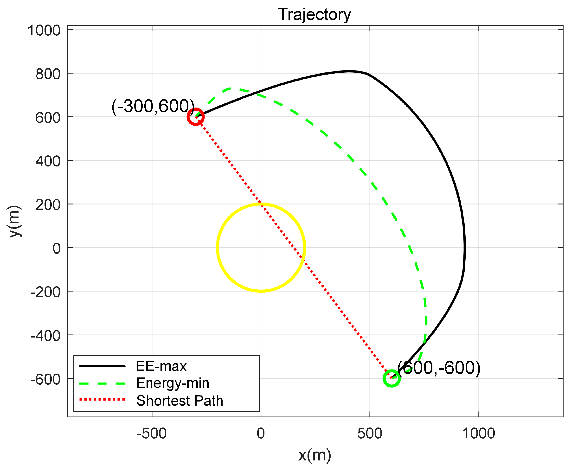
The trajectories with T = 150 s are illustrated in Figure 3. The black curve (labeled “EE-max” in the figure) indicates the UAV trajectory optimized for maximum energy efficiency. For comparison, the red dashed line (labeled “Shortest Path”) represents the shortest path and the green curve is labeled “Energy-min”. The total UAV energy consumption minimization problem was formulated by minimizing the objective function given in Equation (8)) corresponding to the trajectory of an energy-minimize flight. The yellow circle represents the target detection area.

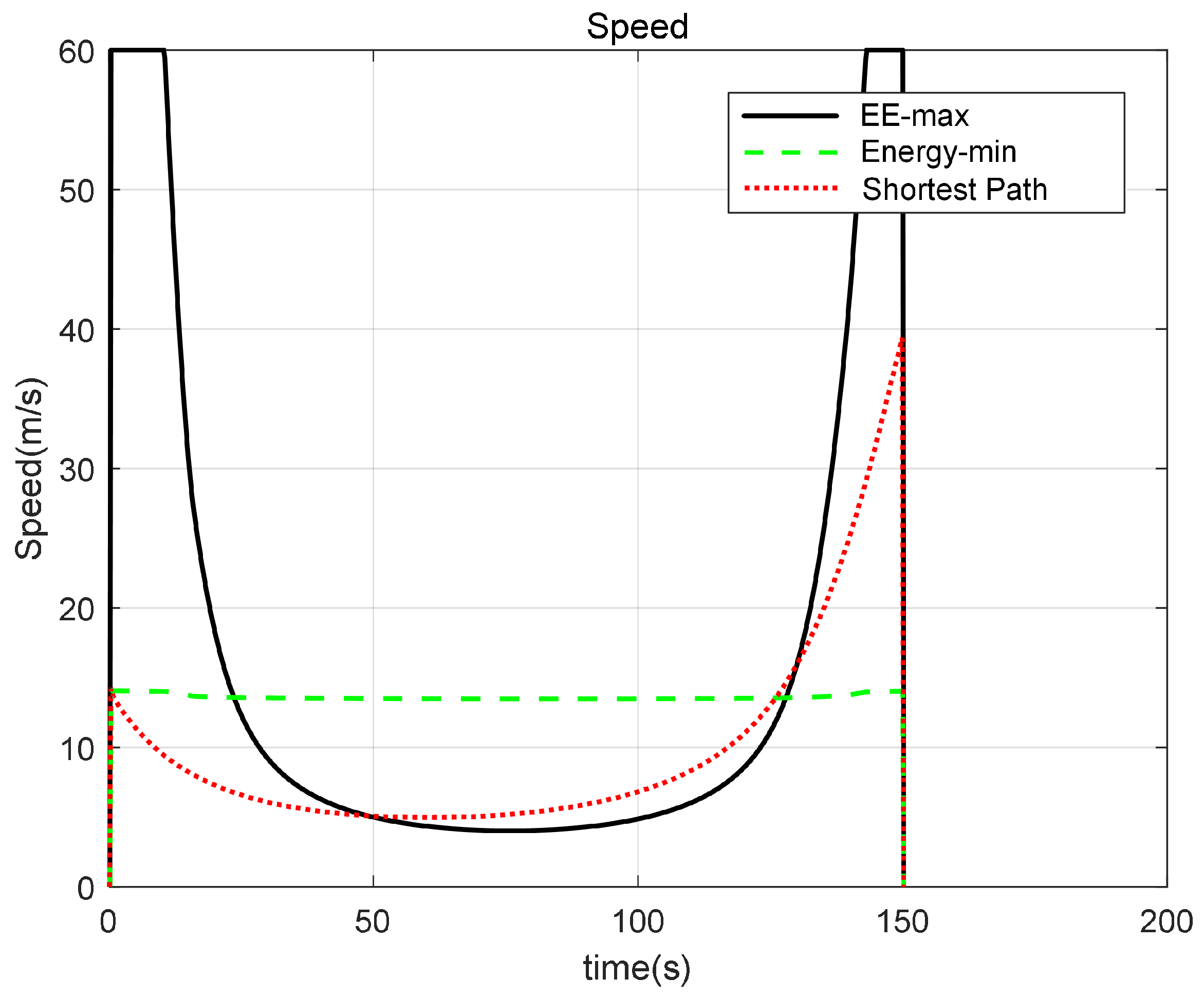
Figure 4 shows the velocities of the three trajectories depicted in Figure 3 as a function of time. It can be observed that for the energy-efficiency-maximizing (EE-max) trajectory, the UAV initially flew outward at a relatively high speed, which increased the distance variation of the received echoes and thereby enhanced the sensing data. Subsequently, the UAV decelerated for a certain period before accelerating again toward the final position. However, for the energy-minimizing trajectory, it can be observed that the UAV followed an approximately uniform-speed motion, with a velocity close to its endurance-maximum speed. This was because the dominant factor affecting the UAV’s total energy consumption was the propulsion energy required for flight. Maintaining the UAV at its maximum endurance speed was an effective strategy to minimize propulsion energy consumption, which consequently reduced the total energy expenditure of the system. For the shortest-path trajectory, the UAV’s velocity first decreased and then increased over time.

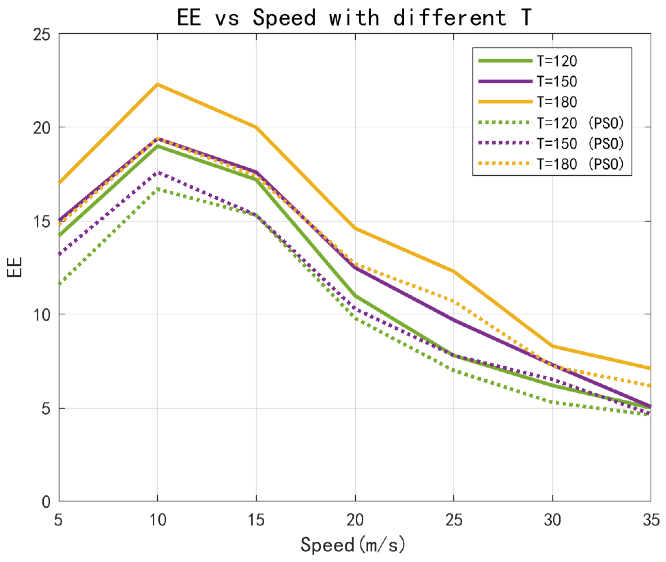
Figure 5 illustrates the relationship between energy efficiency and UAV flight speed under different mission durations T, where the UAV is assumed to fly at a constant speed. It can be observed that as the flight speed increased, the energy efficiency first increased and then decreased, exhibiting a typical non-monotonic trend. For comparison, we also present the results obtained using the Particle Swarm Optimization (PSO) algorithm, with a population size of 100 and a search velocity range set to $[-2,2]$. The six curves represent the energy efficiency under three different flight durations: $T=120\mathrm{s}$, $T=150\mathrm{s}$, and $T=180\mathrm{s}$. Specifically, the solid lines correspond to the proposed method under the three settings, while the dashed lines depict the results obtained by the PSO algorithm for the same durations. As the period T increased, the overall energy efficiency improved. This was because a longer duration allowed the UAV to spend a greater proportion of time flying at a constant speed over the target area, during which the energy efficiency remained relatively stable. The primary variations in energy efficiency occurred during the acceleration and deceleration phases at the beginning and end of the trajectory. Consequently, as T further increased, the energy efficiency at a given speed gradually converged to a steady value. It can also be observed that the proposed method consistently achieved higher energy efficiency than the PSO algorithm under all tested settings.

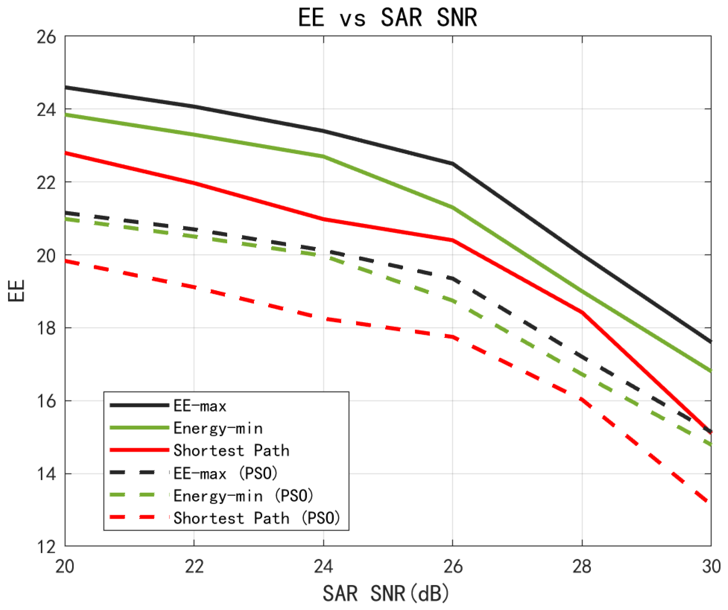
Under fixed system conditions, Figure 6 illustrates the variation in UAV energy efficiency with respect to the SAR SNR for the three considered trajectory designs. Specifically, the solid lines represent the results obtained using the proposed method, while the dashed lines correspond to those derived from the PSO algorithm under the same duration settings.

It can be observed that energy efficiency decreased as the SAR SNR increased. This was because a higher SAR SNR requirement led to increased power consumption in the ISAC system. Furthermore, it can be seen that the proposed method consistently outperformed the PSO algorithm in terms of energy efficiency across all trajectory configurations.

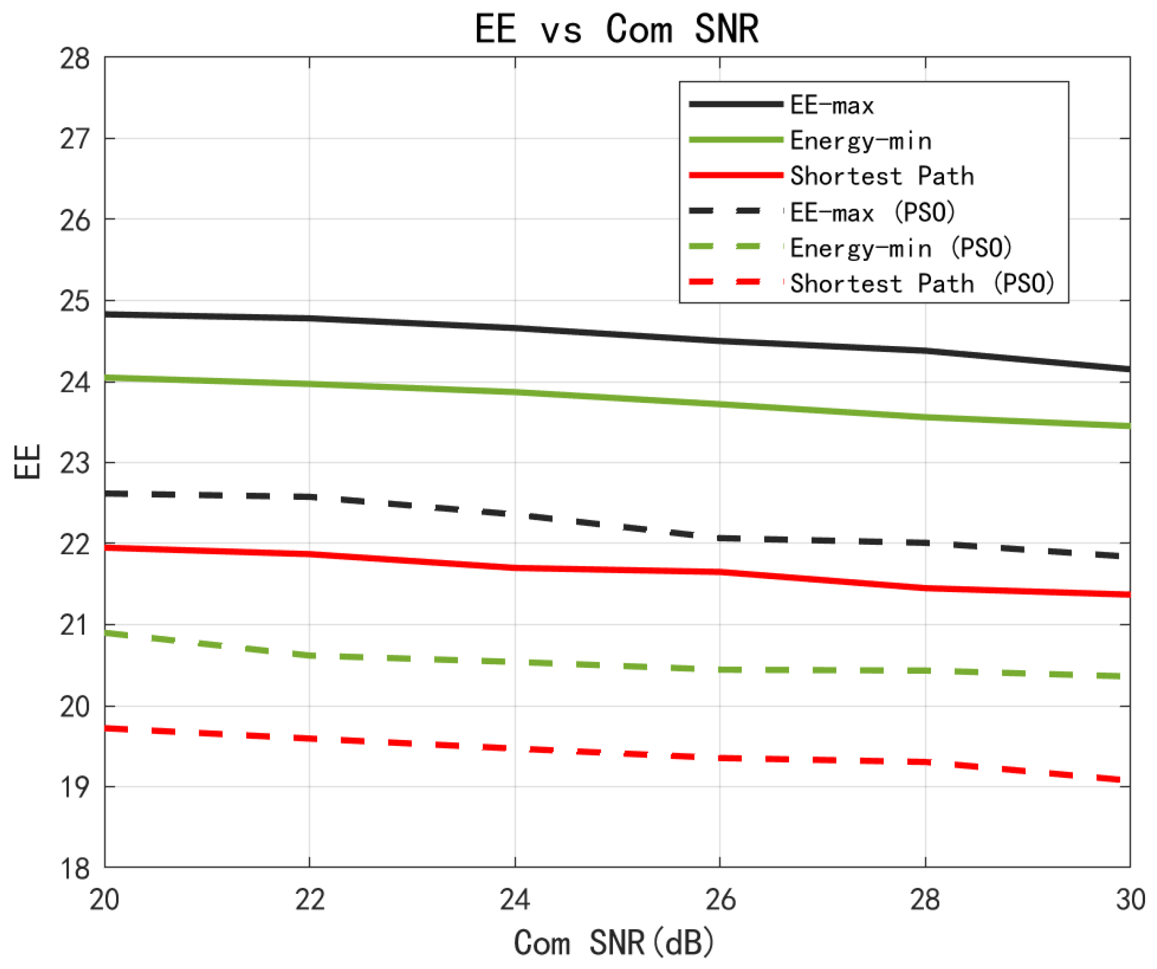
With all other parameters held constant, Figure 7 illustrates the variation in UAV energy efficiency with respect to the communication SNR under three different trajectory designs. The solid lines represent the results of the proposed method, while the dashed lines correspond to those obtained using the PSO algorithm under the same trajectory settings.

It can be observed that the energy efficiency gradually decreased as the communication SNR increased. This was because achieving a higher communication SNR typically required increased transmit power, which led to greater energy consumption. However, since communication-related energy accounted for only a small portion of the UAV’s total energy consumption, the overall decline in energy efficiency remained relatively modest.

In addition, it is evident that the proposed method consistently outperformed the PSO algorithm across all three trajectory configurations in terms of energy efficiency.

The numerical results demonstrate that the proposed algorithm achieved a favorable balance between the UAV’s total energy consumption and the amount of sensed and communicated data, thereby effectively enhancing the overall energy efficiency. Moreover, compared to the PSO algorithm, the proposed method consistently yielded superior performance.

6. Conclusions

This paper presented a comprehensive analysis of the energy efficiency problem in a UAV-SAR-based ISAC system for target area sensing. By jointly optimizing the UAV’s trajectory, velocity, sensing beamforming, communication beamforming, and SAR elevation angle, the energy efficiency of the UAV was significantly improved. Furthermore, a closed-form expression for the UAV’s energy efficiency was derived, and the relationships between energy efficiency and key parameters such as flight speed, SAR SNR, and communication SNR were thoroughly investigated. The effectiveness of the proposed algorithm was validated through simulation results. Compared to the PSO algorithm, the proposed method consistently yielded superior performance. The findings of this work offer valuable insights for UAV-enabled ISAC-based regional imaging, introducing a new perspective: maximizing the amount of sensing data acquired per unit of energy, rather than minimizing energy consumption alone. In the context of regional sensing, the quality and quantity of sensing data are crucial. Pure energy minimization may overlook sensing performance, whereas focusing on energy efficiency facilitates the development of more effective and efficient UAV communication and sensing systems.

Although the results of this study are encouraging, several practical limitations must be considered for real-world deployment. Future research should aim to resolve key engineering challenges in UAV-SAR-based ISAC systems, including ISAC waveform design, system constraint optimization, and the development of real-time UAV control strategies in dynamic environments. Moreover, we plan to incorporate a more refined UAV energy consumption model in future work to enable more accurate and comprehensive performance analysis. Addressing these issues will enhance the feasibility and robustness of the proposed method in complex, real-world scenarios.

References

- Tan, D.K.P.; Choi, J.; Kumari, P.; Abdelhadi, A.; Heath, R.W. Integrated sensing and communication in 6G: Motivations, use cases, requirements, challenges and future directions. In Proceedings of the 2021 1st IEEE International Online Symposium on Joint Communications & Sensing (JC&S), Dresden, Germany, 23–24 February 2021; pp. 1–6. [Google Scholar]
- Inca, S.; Gabbouj, M.; Li, Y.; Rahim, A.; Elakkiya, R. Angular correlation study of sensing and communication channels in V2X scenarios for 6G ISAC usage. In Proceedings of the 2023 IEEE Globecom Workshops (GC Wkshps), Kuala Lumpur, Malaysia, 4–8 December 2023; pp. 1189–1194. [Google Scholar]
- Zhang, J.A.; Rahman, M.L.; Wu, K.; Huang, X.; Guo, Y.J.; Chen, S.; Yuan, J. Enabling joint communication and radar sensing in mobile networks—A survey. IEEE Commun. Surv. Tutor. 2022, 24, 306–345. [Google Scholar] [CrossRef]
- Cui, Y.; Liu, F.; Jing, X.; Mu, J. Integrating sensing and communications for ubiquitous IoT: Applications, trends, and challenges. IEEE Netw. 2021, 35, 158–167. [Google Scholar] [CrossRef]
- Filippone, A. Flight Performance of Fixed and Rotary Wing Aircraft (Butterworth-Heinemann); AIAA: Washington, DC, USA, 2006. [Google Scholar]
- Sekander, S.; Tabassum, H.; Hossain, E. Multi-tier drone architecture for 5G/B5G cellular networks: Challenges, trends, and prospects. IEEE Commun. Mag. 2018, 56, 96–103. [Google Scholar] [CrossRef]
- Rezaei, O.; Naghsh, M.M.; Karbasi, S.M.; Nayebi, M.M. Resource Allocation for UAV-Enabled Integrated Sensing and Communication (ISAC) via Multi-Objective Optimization. In Proceedings of the ICASSP 2023—2023 IEEE International Conference on Acoustics, Speech and Signal Processing (ICASSP), Rhodes Island, Greece, 4–10 June 2023; pp. 1–5. [Google Scholar]
- Cao, L.; Wang, H. Research on UAV Network Communication Application Based on 5G Technology. In Proceedings of the 2022 3rd International Conference on Electronic Communication and Artificial Intelligence (IWECAI), Zhuhai, China, 14–16 January 2022; pp. 125–129. [Google Scholar]
- Chen, Y.; Zhang, S.; Xu, S.; Li, G.Y. Fundamental trade-offs on green wireless networks. IEEE Commun. Mag. 2011, 49, 30–37. [Google Scholar] [CrossRef]
- Ding, Y.; Li, X.; Cai, Y.; Wu, Z. Advancements in ISAC: A review of multi-antenna technology integration for next-generation communication and sensing systems. In Proceedings of the 2024 12th International Conference on Information Systems and Computing Technology (ISCTech), Xi’an, China, 8–11 November 2024; pp. 1–5. [Google Scholar]
- Deng, C.; Fang, X.; Wang, X. Beamforming design and trajectory optimization for UAV-empowered adaptable integrated sensing and communication. IEEE Trans. Wirel. Commun. 2023, 22, 8512–8526. [Google Scholar] [CrossRef]
- Liu, X.; Huang, T.; Shlezinger, N.; Liu, Y.; Zhou, J.; Eldar, Y.C. Joint transmit beamforming for multiuser MIMO communications and MIMO radar. IEEE Trans. Signal Process. 2020, 68, 3929–3944. [Google Scholar] [CrossRef]
- Lyu, Z.; Zhu, G.; Xu, J. Joint maneuver and beamforming design for UAV-enabled integrated sensing and communication. IEEE Trans. Wirel. Commun. 2023, 22, 2424–2440. [Google Scholar] [CrossRef]
- Liu, W.X.; Feng, H.C.; Aye, S.Y.; Ng, B.P.; Lu, Y.L. Design and testing of multi-rotor UAV full-pol SAR system. In Proceedings of the International Conference on Radar Systems (Radar 2017), Belfast, UK, 23–26 October 2017; pp. 1–5. [Google Scholar]
- Wang, D.; Yang, Q.; Liu, Z. Imaging of UAV SAR in Random Azimuth Acceleration. In Proceedings of the 2021 IEEE International Geoscience and Remote Sensing Symposium IGARSS, Brussels, Belgium, 11–16 July 2021; pp. 5131–5134. [Google Scholar]
- Perry, R.P.; DiPietro, R.C.; Fante, R.L. SAR imaging of moving targets. IEEE Trans. Aerosp. Electron. Syst. 1999, 35, 188–200. [Google Scholar] [CrossRef]
- Wang, Y.; Li, J.W.; Sun, B.; Chen, J. Airborne geographically referenced stripmap SAR data processing. In Proceedings of the 2014 IEEE Geoscience and Remote Sensing Symposium, Quebec City, QC, Canada, 13–18 July 2014; pp. 620–623. [Google Scholar]
- Gao, C.; Wang, R.; Deng, Y.; Feng, J.; Yan, H.; Balz, T. Large-scene sliding spotlight SAR using multiple channels in azimuth. IEEE Geosci. Remote Sens. Lett. 2013, 10, 1006–1010. [Google Scholar]
- Hu, S.; Yuan, X.; Ni, W.; Wang, X. Trajectory planning of cellular-connected UAV for communication-assisted radar sensing. IEEE Trans. Commun. 2022, 70, 6385–6396. [Google Scholar] [CrossRef]
- Lahmeri, M.-A.; Ghanem, W.; Knill, C.; Schober, R. Trajectory and resource optimization for UAV synthetic aperture radar. In Proceedings of the 2022 IEEE Globecom Workshops (GC Wkshps), Rio de Janeiro, Brazil, 4–8 December 2022; pp. 897–903. [Google Scholar]
- Li, K.; Ni, W.; Wang, X.; Liu, R.P.; Kanhere, S.S.; Jha, S. Energy-efficient cooperative relaying for unmanned aerial vehicles. IEEE Trans. Mobile Comput. 2016, 15, 1377–1386. [Google Scholar] [CrossRef]
- Zeng, Y.; Zhang, R. Energy-efficient UAV communication with trajectory optimization. IEEE Trans. Wirel. Commun. 2017, 16, 3747–3760. [Google Scholar] [CrossRef]
- Sun, C.; Xiong, X.; Ni, W.; Wang, X. Three-dimensional trajectory design for energy-efficient UAV-assisted data collection. In Proceedings of the ICC 2022—IEEE International Conference on Communications, Seoul, Republic of Korea, 16–20 May 2022; pp. 3580–3585. [Google Scholar]
- Ahmed, S.; Chowdhury, M.Z.; Jang, Y.M. Energy-efficient UAV relaying communications to serve ground nodes. IEEE Commun. Lett. 2020, 24, 849–852. [Google Scholar]
- Zhang, S.; Cao, R.; Jiang, Z. Energy-efficient data collection and trajectory design for UAV-enabled wireless sensor network. In Proceedings of the 2022 IEEE 5th International Conference on Electronics Technology (ICET), Chengdu, China, 13–16 May 2022; pp. 933–938. [Google Scholar]
- Younis, M. Digital Beam-Forming for High Resolution Wide Swath Real and Synthetic Aperture Radar. Ph.D. Thesis, University of Karlsruhe, Karlsruhe, Germany, 2004. [Google Scholar]
- Kim, S.Y.; Myung, N.H.; Kang, M.J. Antenna mask design for SAR performance optimization. IEEE Geosci. Remote Sens. Lett. 2009, 6, 443–447. [Google Scholar]
- Zeng, Y.; Xu, J.; Zhang, R. Energy minimization for wireless communication with rotary-wing UAV. IEEE Trans. Wirel. Commun. 2019, 18, 2329–2345. [Google Scholar] [CrossRef]
- Crouzeix, J.-P.; Ferland, J.A. Algorithms for generalized fractional programming. Math. Program. 1991, 52, 191–207. [Google Scholar]