Abstract
To tackle the challenges of unknown image distortion and catastrophic forgetting in incremental inverse synthetic aperture radar (ISAR) target classification, this article introduces a deformation-robust non-exemplar incremental ISAR target classification method based on the Mix-Mamba feature adjustment network (MMFAN). The Mix-Mamba backbone employs channel-wise spatial transformations across multi-scale feature maps to inherently resist deformation distortions while generating compact global embedding through Mamba vision blocks. Then, the feature adjustment network facilitates knowledge transfer between base and incremental classes by dynamically maintaining a prototype for each target class. Finally, the loss bar synergizes supervised classification, unsupervised adaptation, and prototype consistency enforcement, enabling stable incremental training. Extensive experiments on ISAR datasets demonstrate the performance improvements of incremental learning and classification robustness under scaled, rotated, and mixed deformation test scenarios.
1. Introduction
Thanks to the advantages of day-and-night, all-weather and long-range capability, inverse synthetic aperture radar (ISAR) has played an important role in maritime surveillance, space situational awareness, and air defense early warning [1,2,3]. Essentially different from optical imaging, which relies on vertical projection of the target-reflected light along the observation direction, ISAR captures the horizontal projection of target electromagnetic scattering centers along the radar line-of-sight (LOS). This fundamental distinction enables ISAR to extract target shape and size characteristics that complement optical imagery, particularly for non-cooperative targets with dynamic trajectories [4]. Hence, high-precision air/space target classification based on two-dimensional (2D) ISAR images becomes a research hotspot in the community of radar systems [5,6,7,8].
As a range–Doppler image, the range resolution of the ISAR image is determined by the time–bandwidth product of the transmitting waveforms, while the azimuthal resolution is determined by the relative rotation angle between the target and radar [9]. This particular imaging property therefore causes severe unknown deformation distortions (such as scaling and rotating) [10]. Furthermore, the non-cooperative target and the unknown imaging projection plane (IPP) render traditional classification methods scarcely able to correct these deformations directly by parameter estimation [11]. Hence it is urgent to investigate ISAR deformation-robust feature extraction frameworks that can adapt to unknown imaging distortions without prior parameter calibration. Motivated by the global dynamic access of the Mamba network and the inherent unknown deformation distortion of ISAR imaging, this article proposes a Mix-Mamba backbone incorporating channel-wise spatial trans-formation and Mamba vision to directly adjust and encode image deformations in the feature domain.
Another property of ISAR target classification is the continuous acquisition of target samples. Although data-driven deep-learning methods have recently improved the accuracy and generalization of computer vision tasks, their effectiveness still relies on careful training utilizing large-scale datasets [12]. In practice, however, the acquisition of ISAR datasets is an ongoing process along with space launch and radar detection, and new targets and samples are supplemented throughout the model’s lifelong training and deployment. Conventional methods fine-tune the model directly on the new class data, which will suffer from catastrophic forgetting, i.e., a dramatic performance degradation due to the overwriting of old-task knowledge. While exemplar-based incremental learning methods alleviate this issue by retaining some of the reference samples [13,14,15,16,17,18,19], they incur prohibitive computational costs and security risks, with ISAR handling sensitive defense data. Thus, developing a non-exemplar class-incremental classification method is fundamental for the realization of a practical automatic ISAR system. In this article, the feature adjustment network (FAN) is proposed to dynamically align feature spaces across incremental tasks through maintaining prototypes without storing raw ISAR images.
1.1. Prior Work
Traditional ISAR target classification methods represent and classify features of 2D images by manually constructing templates, target models, or classifiers [20,21,22], but their performance is severely limited in terms of accuracy, model capacity, and migration generalization. For unknown image deformation, traditional methods (1) extract deformation-robust features directly in the image domain, e.g., by using the Cloude–Pottier decomposition to extract orientation and motion invariant features of the scattering points [23], or extracting simplified shape matrix features independent of target scaling, translation, and rotation [24]; (2) map the ISAR images to transform domain, which is invariant to rotation and translation, and then extract features and perform classification, e.g., polar mapping [25] and trace transformation [26]; and (3) estimate the target rotational speed for Doppler calibration [27,28] so as to obtain an azimuth-corrected ISAR image [22]. However, these methods exhibit several limitations, including the loss of critical target shape and structural information, stringent requirements for Doppler calibration, and significant azimuth estimation errors.
Recently, deep-learning methods such as convolutional neural networks (CNNs) [29], including Long Short-Term Memory (LSTM) [8] and Vision Transformer (ViT) [30], have been proposed to obtain high accuracy and strong generalization in ISAR target classification networks. They can automatically extract features from a large-scale dataset, eliminating the tedious manual feature designing. Nevertheless, the conventional deep networks exhibit critical limitations in handling ISAR unknown deformations. For instance, CNNs, constrained by fixed receptive fields, struggle to reconcile localized distortions (stretched edges or anisotropy scattering centers) with global context. While transformer-based models treat all image patches as equally important, they overlook the inherent anisotropy of ISAR imaging, where deformation patterns exhibit spatial correlations across scales. Moreover, ViTs leverage self-attention mechanisms to model global dependencies, and their quadratic complexity and defect of inductive bias fail to capture ISAR spatial variations efficiently [31]. RetentiveNet [32] introduces a multi-scale retention mechanism into Transformers, which breaks the “training parallelism—memory efficient—long sequence” trilemma through a combination of parallel representation, recurrent encoding, and block-wise recursion. While maintaining the performance of Transformers, it achieves linear inference complexity.
State-space models (SSMs) describe dynamic systems through the mapping relationship between inputs and state variables. To address the issue of SSMs in long sequence modeling, structured state space (S4) [33] incorporates HiPPO initialization to solve the long dependence issue and structurally decomposes the state transition matrix to improve numerical stability. Structured state space for diagonal matrices (S4D) [34] forcibly constrains the state matrix of S4 into a diagonal structure. It significantly reduces the number of trainable parameters by simplifying the 2D convolution kernel into two 1D convolutions, while still maintaining the ability to capture long-range dependencies. Mamba [35] is an advanced SSM that inherits the HiPPO matrix decomposition of S4D but further enables the state matrix and step size to adaptively adjust according to the input content, which achieves dynamic selection of information compression. Mamba also introduces parallel scanning algorithms and kernel fusion techniques to enable a multiple-fold increase in inference speed. Inspired by the architecture of ViTs, Vision Mamba [36] replaces the transformer encoder with a Mamba encoder while retaining the process of linear mapping of 2D images into vectors. Unlike Transformers, which rely on static attention maps, Vision Mamba dynamically adjusts feature interactions through parameter-efficient sequential processing, and it is emerging as a prominent backbone network for visual tasks.
For ISAR’s unknown deformation distortion, prior methods can be divided into two aspects, namely data augmentation and deformation adjustment. The data augmentation methods extend the coverage of the data space by introducing auxiliary datasets; i.e., the images in the training set are randomly scaled, rotated, flipped, translated, and cropped [37] to increase the feature patterns experienced by the network training. However, data augmentation also increases the training cost of the network, fails to generate new target classes, and lacks interpretability. Deformation adjustment methods, such as deformable convolution [38], adjust the shape of the feature maps through local offsets of the receptive field. Moreover, the spatial transformation network (STN) estimates the global affine transformation parameters of the input image to adjust the image in the direction of reducing training losses [39]. However, only adjusting the original image in STN has two issues: (1) Feature mismatch: Arbitrary image scaling and rotation induce spatial misalignment between local features and global structures. After spatial transformation, the feature maps of the transformed image may not be aligned with the feature maps of the original image [40]. (2) Shape mismatch: Multiple target shapes can be conducive to classification. Keeping only one form of transformation result will mismatch a better target shape and even lose local information of the original images [7].
For class incremental learning, the existing methods can be divided into three categories:
- Data replay: To address the issue of catastrophic forgetting, data replay methods focus on extracting common information from preceding task exemplars. Incremental classifier and representation learning (iCarl) [13] firstly introduces dynamic sample replay, where the representative samples are selected from the feature space according to the nearest-mean-of-exemplar rule, and the exemplar library is dynamically updated using a herding algorithm to maintain learning stability. Based on iCarl, enhancement methods are proposed involving dynamically adjusting the number of exemplars, class-balanced sampling, and parameterized exemplars, respectively [14]. Furthermore, instead of saving a large number of samples, generative models such as the generative adversarial network (GAN) [16], conditional GAN [17], and diffusion models [18] can be trained to obtain pseudo old-class samples. Additionally, preserving the extracted features of the old-class samples could also maintain the decision boundaries of the previous tasks, thus reducing the memory expenditure [19]. For radar target classification, Zhao et al. [41] propose an orthogonal feature distribution optimization combined with random augmentation of high-dimensional features to preserve partial detailed features of base classes, thereby achieving incremental learning for few-shot SAR images. As for radar ship target detection, ref. [42] combines the contextual robust exemplar replay and multi-granularity knowledge distillation. Based on the preliminary land–sea separation, regional data replay is carried out so as to transfer the knowledge of the old model step-by-step and realize the smooth transition of incremental samples. However, feature-based data replay methods are subject to changes in feature representation during model updating, leading to feature drift and class conflation.
- Dynamic structure: To maintain the performance on both old- and new-class data, dynamic structure methods freeze the old network parameters and expand a subnetwork for each incremental task. Progressive neural networks (PNNs) [43] and dynamically expandable representation (DER) [44] replicate and fine-tune the backbone network for each new task and then expand the full connection layer to accommodate greater model capacity. Ref. [45] partially expands the stability and plasticity network modules and aggregates their inference results to enhance the model’s representation capability. To address the issue of dramatic memory increase from backbone expansion, the memory-efficient expandable model (MEMO) [46] decouples the deep and shallow features of the backbone network and builds a dedicated deep block for each task to achieve a balance between memory and performance. The feature boosting model (FOSTER) [47] compresses the model to limit the number of backbone networks and reduce parameter redundancy. Ref. [48] proposes a dynamic structure reorganization strategy to make room for new tasks by constructing network side branches, and the side branches are rearranged to the main branch through a reparameterization technique, ensuring a constant number of network parameters. However, dynamic structure methods increase the complexity of the model, which will affect the model’s efficiency and scalability, especially when dealing with large datasets or using deep backbones.
- Model regularization: To protect the learned knowledge from being overwritten by new class data, model regularization methods impose various constraints on the class-incremental learning model. Among them, parameter regularization methods consider that each parameter contributes differently to the learning task and combats catastrophic forgetting by retaining partially significant parameter knowledge. The importance of parameters can be estimated by the Fisher information matrix [49] or online synaptic calculation [50], and parameter constraint can be realized by a Bayesian framework or hierarchical network constraint [51], but such methods still suffer from linearly increased memory with the class samples. Another approach is function regularization, which maintains model stability by constraining the outputs of the old and new models corresponding to the same input sample. Learning without forgetting (LwF) [52] and bias correction (BiC) [53] take the output of the old model from new tasks as a reference and optimize the new model by adding a knowledge distillation loss. This prevents the performance degradation of the old classes due to over-reliance on the new-task learning. In addition, the network intermediates can also be utilized for feature distillation, such as the feature vectors from the backbone network [54], multi-layer pooling features [55], and attention maps of the classifiers [56]. DS-AL [57] proposes a dual-stream analytical learning method. The main stream provides an analytical linear solution, while the compensation stream improves the underfitting limitation inherent in linear mapping. For SAR images, ref. [58] proposes a non-exemplar incremental learning method based on mutual information maximization. By actively clustering features, the distribution overlap caused by inherent small inter-class differences and large intra-class variances in SAR images can be avoided. However, model regularization methods rely on the correlation among tasks, and model parameter updates will lead to task confusion if the incremental data varies greatly.
1.2. Contribution
To tackle the issues of unknown deformation vulnerability and exemplar-preserving overhead, this article proposes a Mix-Mamba feature adjustment network (MMFAN) for robust non-exemplar class-incremental ISAR target classification. The Mix-Mamba is designed as the backbone to obtain embedding features, and it consists of channel-wise spatial transformation (CST) and Mamba vision techniques that perform multi-layer feature map deformation adjustment and global feature extraction, respectively. Then, a prototype vector is maintained for each class of samples, and the embedding features and prototypes are fine-tuned by a FAN during each incremental task, thereby achieving non-exemplar incremental classification. The loss bar is constructed to fuse multiple loss functions so as to strike a balance between new-class plasticity and old-class stability. Unlike conventional methods that either rely on exemplar preservation or suffer from deformation-induced performance degradation, MMFAN establishes a deformation-robust and data-safety paradigm through three main contributions:
- CST is proposed for deformation-robust feature extraction. Traditional STNs assume uniform spatial transformations across the entire image, ignoring ISAR local distortion variability. CST independently performs deformation parameter estimation and homography transformation on multi-layer and multi-channel feature maps, enabling localized adjustments tailored to distinct deformation patterns at different scales.
- A Mix-Mamba backbone network is proposed for bridging CNN localities and Mamba global contexts. CNNs struggle with ISAR large-scale deformations due to fixed receptive fields, while ViTs face parameter redundancy and training instability under limited ISAR samples. Mix-Mamba leverages cross-scale information propagation of SSMs to adaptively adjust features to varying distortion levels, aligning with ISAR’s inherent varied resolution imaging physics.
- A FAN is designed for non-exemplar incremental learning. FAN introduces dynamic prototype maintenance that represents the old class targets on the new task, so that the forgetting of the historical knowledge caused by new-task learning can be decreased without saving any sample exemplar. The loss bar is also applied to fuse the distillation loss and feature adjustment loss to ensure the stability of network training.
The remainder of the article is organized as follows: Section 2 provides a detailed structure and module inference process of MMFAN. Section 3 provides the datasets, results, and analysis of the incremental learning experiments. Section 4 discusses the experimental results and outlines the future work directions. Finally, Section 5 concludes the article.
2. MMFAN Methods
In this section, we first provide the definition of class-incremental target classification and then introduce the detailed network structure and learning procedures of MMFAN.
2.1. Problem Definition
Without loss of generality, the data sequence of class-incremental learning includes T groups of classification tasks , where is the t-th incremental task, is the number of training samples in task t, represents the ISAR image sample, and denote the width and height of the image, respectively. The class label of the sample is shown as , where denotes the label space corresponding to task t. The label spaces do not overlap between tasks, i.e., for . During the training task t, the model can only access data , and the goal of class-incremental learning is to establish a classifier for all the classes by continuously learning the new knowledge from T tasks. After the training of task t, MMFAN maintains a prototype library of known classes, which is then validated on all test sets from task 1 to t, where is a prototypical vector of dimension . The ideal class-incremental learning model not only performs well on the newly learned classes for task t, but also needs to retain memory for historical classes, i.e.,
where H denotes the parameters of model and is an indicator function, i.e., it outputs 1 if the condition is satisfied, otherwise 0. represents the test data for task t and is subject to deformation distortion. The training samples do not intersect with the test samples, i.e., . As a non-exemplar class-incremental learning framework, MMFAN can only access and the prototypes during the training of task t and also retains deformation robustness to test samples.
2.2. Overall Structure
The overall structure of MMFAN is shown in Figure 1, which can be divided into three parts: the Mix-Mamba backbone, FAN, and the loss bar. The Mix-Mamba backbone extracts the embedding features from the input samples and memorizes historical information by the prototypical vectors. FAN transfers the embedding features and prototypes between different tasks. The loss bar fuses five different loss functions to form a prototype-guided and non-exemplar incremental training procedure that guides the parameter updating of Mix-Mamba and FAN. In Figure 1, the dotted and solid trapezoids represent the parameters of the Mix-Mamba backbone in task t − 1 (old) and task t (new), respectively. In the embedded feature zone, solid squares represent embeddings extracted by the original input images, slash squares represent embeddings extracted by the augmented input images, stars represent prototypes generated from embedded features, and pentagrams and squares with the same color correspond to the same target category. The blue arrows denote the generation and update flow of the prototypes, while the black arrows denote the data flow for network training.
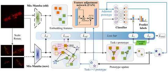
Figure 1.
Overall process of the MMFAN incremental ISAR target classification.
Take task t as an example for generally describing the training and test of MMFAN. First, the parameters of Mix-Mamba in task t − 1 are fixed and copied as the old backbone (which does not involve gradient calculation) to serve as a reference for the historical memory. The new backbone participates in all gradient backpropagation and parameter updating and obtains classification results. Then, the input image is fed into both the old and new backbones to obtain the embedding features and , respectively. In order to constrain the new model from overfitting to the distribution of new classes, the distillation loss is calculated to minimize the difference between the features extracted by the old and new models, both from a new sample. For the new model, the augmented input samples (by scaling and rotating on ) are fed into the new backbone to obtain augmented features . Then and the historical prototypes serve as a contrastive learning template for supervised contrastive learning with , obtaining a contrastive loss .
FAN plays the role of transferring the feature distribution from the old backbone to the new backbone, i.e., . To achieve a better proximity between the adjusted features and the new backbone features, the feature adjustment loss is designed to minimize the difference between and . Another role of FAN is to adjust prototypes corresponding to all learned classes, thus mapping the old-class prototypes to the new feature space, i.e., . Then, the adjusted prototypes are input into the classifier to obtain the predicted prototype label, and the prototypical loss is computed by comparing the prototype label with the true class label. The features extracted by the new backbone are also fed into the classifier, and the classification loss is obtained by comparing them with the true class labels. Finally, the mean of corresponding to each class is computed to obtain the new class prototype for task t, which is then combined with to update the prototype library as .
2.3. Mix-Mamba
The network structure of Mix-Mamba is shown in Figure 2, which is composed of three CST convolution stages and two Mamba stages. Compared with the original Mamba, Mix-Mamba mainly increases the CST convolution as a deformation-robust structure; in addition, motivated by Vision Transformer, Mix-Mamba uses the Mamba vision block to extract global features as 2D feature maps. As a backbone, Mix-Mamba takes image samples as input and obtains embedding vectors with the dimension of . Due to the spatial inductive bias and strong local feature-extraction capabilities of convolutional networks, the CST convolution stages with residuals are designed to extract high-resolution features while adjusting deformations such as scaling, rotation, and perspective distortion in the feature maps. Mamba stages divide the feature maps into patches and employ selective scanning structured state-space models (S6M) [59] for global context modeling, thus overcoming the limitations of capturing global spatial relationships for convolutional networks.
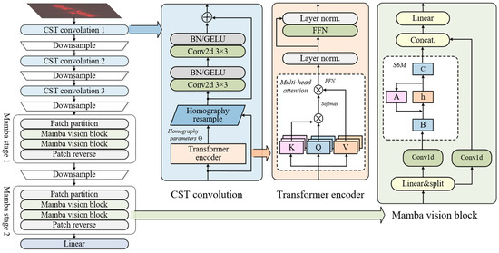
Figure 2.
Network structure of Mix-Mamba.
CST convolution stage: the CST operation illustrates three improvements over the original STN to figure out feature mismatch and shape mismatch: (1) introducing a more flexible homography transformation instead of the affine transformation [60], (2) applying spatial transformations independently to multi-layer and each channel features, and (3) generating transformation parameters through a Transformer encoder rather than a simple linear function. By utilizing the cross-attention mechanism, the homography parameters are extracted from the image features through the learnable query vector. For the input feature map , where H and W represent the height and width of the feature map and C is the number of channels, the Transformer encoder calculates the attention scores by scaled dot-product attention. Let the attention value V and key K be obtained through linear mappings, while letting the query Q be a learnable parameter for querying a preset length of output from the feature. We denote as the hidden dimension of the Transformer encoder, as a two-layer fully-connected network followed by the Gaussian error linear unit (GELU) non-linear activation function, as the linear mapping from the feature dimension to , and as the layer normalization, then the homography parameters are obtained by
where the homography transformation parameters are extracted from the image features through the learnable query vector by using the Transformer cross-attention mechanism.
After obtaining , it can be rearranged as C groups of individual 3 × 3 transformation matrices according to the homogeneity, and then each channel of the feature maps can be resampled. The homography transformation can map the projections of 3D scatter points between different IPPs, thereby enabling the adjustment of the unknown deformation of ISAR images. Specifically, it calculates the pixel at position in the output feature map corresponding to the position in the input feature map , where . Then, the output pixel value of the channel c is obtained by bilinear interpolation as follows:
In each CST convolution stage, the adjusted feature map is then fed into a two-layer 3 × 3 convolutional network () for local feature extraction, where each convolutional layer is followed by batch normalization (BN) and a GELU activation. Finally, the output of the CST convolution stage is realized by element-wise adding the adjusted feature map for residual connecting, which is down-sampled by a 2 × 2 max-pooling () with doubled channel size, i.e.,
Mamba stage: The global feature extraction is realized by patch partition/reverse and two Mamba vision blocks [61]. The feature map is firstly partitioned (denoted by ) into NC non-overlapping patches of size , where , and these patches are then flattened into vectors of length , which is then linearly mapped and added with a learnable positional encoding to obtain the patch embedding sequence as
where d denotes the feature dimension of this layer, and denotes the process of patch partition.
In the Mamba vision block, the patch embedding sequence is firstly linearly expanded along feature dimension from d to 2d, then it is split into two streams (denoted as ) with the same size: the Mamba flow and the residual flow , i.e.,
The Mamba flow consists of a 1D convolution with a kernel size of 3 (denoted as ), a sigmoid linear unit () activation, and an S6M operation (denoted as ). Conversely, the residual flow maintains the same structure without the S6M operation to preserve the local spatial relationships. Thereafter, the outputs of both streams are concatenated along the feature dimension (denoted as ) and linearly mapped back to the original dimension d as
In order to recover the feature maps, the output of Mamba vision block is obtained by linear mapping and patch reverse (denoted as ):
Finally, the feature downsampling and channel doubling are realized in the same way as (4). After the last Mamba stage, a global average pooling layer is designed to obtain the embedding feature vector corresponding to the input ISAR image.
In the Mamba vision block, S6M is the core for global feature extraction and contextual representation, which is improved from the SSM. The SSM handles long-term dependencies through sequence-to-sequence mappings and maintains a set of hidden state spaces to predict the output. For a 1D sequence , where and is the sequence length, the continuous SSM defines the linear mapping from the input to the hidden state and output as
where denotes a state transition matrix that governs the retention of the , denotes an input matrix that governs the update of , and denotes the output matrix that governs the contribution of the to the output. M is the dimension of the state space. Under the framework of deep learning, the continuous model is computationally inefficient and hard to train, so the SSM is discretized by converting the derivative into differences and aligning with the data sampling rate. The zero-order hold technique [62] preserves the discrete data for a certain period and generates continuous output during that period. The preservation period is referred to as the sampling timescale , and the discrete SSM takes the form of
where
To embed the discrete SSM into a deep network, the state updating can be expanded along the time dimension and implemented by a 1D convolution, i.e.,
where is the convolution kernel. Therefore, the discrete SSM can be realized in parallel during training via convolution and al retain memory capability like a recurrent neural network (RNN). However, SSM is linear time-invariant, i.e., are static parameters, and their values do not directly depend on the input sequence. It limits the capability of long-term dependencies and global representations. Hence, S6M introduces selective scanning to grant the hidden states the ability to select content based on the input data. In the selective scanning, the step size , the matrix , and are derived from the parallelized input sequence as follows:
where ensures that the timescale is positive, and is the dimension of the selective scanning.
2.4. FAN
As a bridge between the distributions of old and new class features, FAN transfers the old-class prototypes to the feature space of the new tasks, thereby relieving catastrophic forgetting caused by prototype mismatch. Let the backbone network of task t − 1 and task t generate embedding features and , respectively, from the same sample of task t, where and are the corresponding feature spaces formed by all possible features. To transfer the distribution of to with minimal cost, the optimal transportation model is established due to the discrete form of the Monge formula:
where is the optimal transport function that minimizes the cost, is the measure-preserving mapping of transporting from the feature space to , and denotes the cost function transferring to ; here, it can be represented as the Wasserstein distance between the features transferred by the old and new backbones, i.e.,
In order to realize end-to-end model training, the proposed FAN is also implemented by a Transformer encoder, as shown in (2), and the self-attention mechanism is applied here to obtain the internal relationship between old and new embedded features, thereby realizing the transfer of feature distribution. The parameter of FAN is optimized by the feature adjustment loss and prototype loss together.
2.5. Network Training
In the context of non-exemplar incremental learning, to alleviate the conflict between catastrophic forgetting and new-task learning, MMFAN combines feature replay and knowledge distillation techniques [63]. The loss bar is proposed for prototype-guided and non-exemplar network training, where the supervised classification loss , contrastive loss , prototype loss , unsupervised distillation loss , and feature adjustment loss are weighted and summed as follows:
where are the weights for each loss.
Classification loss: It measures the accuracy of the class label predictions by the Mix-Mamba backbone and the linear classifier , fulfilled by the following cross-entropy loss function:
where K is the total number of classes, and denotes the true class label.
Contrastive loss: It helps the backbone to compress the feature space and separate the different classes in incremental tasks. Since the historical data cannot be accessed, in the new feature space, the prototypes corresponding to old classes may be overlapped with the features extracted by the new backbone, increasing the error of decision boundaries. For a batch of input samples, the corresponding embedding features are noted as a set , while the features of augmented samples are noted as a set . The supervised contrastive loss takes as a reference, with the features in that share the same class as the reference are positive samples. In contrast, the prototypes in and features in longing to different classes of are considered negative samples. Consequently, the inner product of features is employed to quantify the similarity between positive and negative samples thus:
where and are the labels corresponding to and , denotes the number of the samples in with the same class label as , and denote the temperature coefficient. In (18), the numerator encourages the features with the same class to come closer (reducing intra-class distance), while the denominator encourages pushing away the features with different classes (increasing inter-class distance). Therefore, the supervised contrastive loss prevents the dispersed feature distribution of new samples, thus mitigating the failure of historical decision boundaries and knowledge forgetting.
Prototype loss: measures the precision of the classification result from the prototype adjusted by FAN, which is realized by a cross-entropy function as
where is the ground true of the prototype. Prototype loss ensures that the classifier enables discriminability for the adjusted old-class prototypes.
Distillation loss: directly computes the L2 distance between the embedding feature extracted by the old backbone and the new backbone , i.e.,
The distillation loss enables the new backbone to recover the historical knowledge.
Feature adjustment loss: As an unsupervised loss, is designed to optimize FAN such that the prototypes can be mapped to an appropriate place in the new feature space, thus reducing the mismatch between the prototype and feature during cross-task incremental learning. Specifically, calculates the L2 distance between the adjusted feature of the old backbone and the feature of the new backbone, i.e.,
3. Experiments and Results
In this section, we present the class-incremental classification experiments of the proposed MMFAN, including the ISAR image dataset configuration, implementation details, algorithm comparisons, ablation study, real-world data experiments, and experiments for learning from scratch. All experiments and comparison results are based on an RTX 5000 mobile GPU (304 CUDA cores, 16 GB GDDR6 memory), Intel i9-11950H CPU, 64 GB system memory, and the software configurations are Python 3.11/PyTorch 2.1.2 with CUDA 12.1.
3.1. Datasets
To validate the performance of the proposed MMFAN, an ISAR image dataset with seven classes of satellite targets [7] is constructed, which consists of CALIPSO, Jason-3, IceSat, QuikSCAT, OCO-2, Cloudsat, and SWAS. Firstly, a local coordinate system for each target is established. Based on the physical-optical theory, the HV-polarized echoes of the target 3D models are generated by electromagnetic computing at the 17 GHz radar carrier frequency and bandwidths of B = 1, 1.5, and 2 GHz, respectively, where the target elevation angles are set as 50° and 55° and azimuth angles are varying from 0° to 360° with a step of 0.02°. Then, ISAR imaging is performed by the back-projection algorithm [64], where azimuth accumulation angles are set to 4, 5, and 6°, and the azimuth interval between images is 1°. Therefore, 360 ISAR images are obtained for each class for a combination of . The ISAR images are finally centered around the target and cropped to the size of 120 × 120 pixels. Figure 3 shows the optical and ISAR image samples for the seven targets.
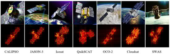
Figure 3.
Optical and typical ISAR image samples of the satellite targets.
For incremental learning, the dataset is divided into four tasks by target class according to Table 1, where Task 1 (the base task) consists of four targets, and Tasks 2–4 (incremental tasks) each add one more target to the previous task. For non-exemplar training, Task t is only allowed to access the current training data, while the test process requires predicting all samples from Task 1 to t, so as to evaluate the model’s resistance to catastrophic forgetting.

Table 1.
Incremental learning task configurations.
To evaluate the robustness of the proposed MMFAN to unknown deformations of ISAR images, four test scenarios are generated with different training and test distortions. As shown in Table 2, the normal scenario only illustrates different elevation angles for the training and test data; in the scaled scenario, the training and test data have different combinations of while sharing the same azimuth angle ; in the rotated scenario, the training and test data share the same combination of while having different elevation and azimuth angles , where the training data has the deficiency of 0–90° azimuth samples; and the combined scenario includes both the scaled and rotated distortions.
Table 2.
Experiment configurations.
3.2. Implementation Details
In this article, the channel size of the initial layer of MMFAN is set to 32. Then each downsampling layer doubles the number of channels, thus obtaining the output embedding features with the dimension of . For the Transformer encoder, the hidden dimension is set to twice the feature dimension in the corresponding layer. For the Mamba vision block, the patch size P = 4, the state-space dimension M = 16, and the temperature coefficient of the contrastive loss is = 0.07. For training MMFAN, we apply the Lamb optimizer [65] with an initial learning rate of 0.002 and cosine decay of 10−5, and the weight decay coefficient is 0.0001. In each incremental task, the MMFAN has 100 training epochs with a batch size of 64, and then it is evaluated on all historical tasks of test data.
3.3. Experimental Results
The accuracy of MMFAN under normal, scaled, rotated, and combined test scenarios for class-incremental learning experiments is shown in Table 3, where the accuracy for Tasks 1–4 is evaluated on all test samples up to the current task, and the average accuracy represents the mean result across the four tasks. It can be seen that the average accuracy in the normal scenario is 91.82%. In the combined test scenario, due to the coupling of scaled and rotated distortions, training and test samples have increased distribution differences. Despite this, MMFAN still achieves an average accuracy of 87.23%, indicating that the proposed CST can effectively resist the performance decline caused by unknown image deformations. The confusion matrices for Task 4 in different test scenarios are shown in Figure 4. It can be seen that, after three new learning tasks, the target classes in the initial task still maintain a high accuracy, demonstrating that the MMFAN balances well between learning new categories and retaining old memories.
Table 3.
Mean accuracy and confidence of different test scenarios.
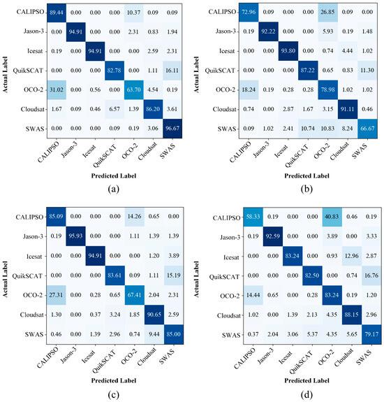
Figure 4.
Confusion matrices (%) of different test scenarios. (a) Normal scenario. (b) Scaled scenario. (c) Rotated scenario. (d) Combined scenario.
To further demonstrate the incremental effectiveness of MMFAN, the embedding features in each task are visualized by t-distributed stochastic neighbor embedding (t-SNE) [66], as shown in Figure 5. The points in different colors represent the 2D projections of features from different targets. Compared with the feature distribution of Task 1, MMFAN pushes the newly added target samples in Task 2 to 4 as far away from the old targets as possible to avoid target confusion between tasks. Furthermore, although exemplars were not retained in incremental learning, the feature distribution of the old targets still changed after each task. It demonstrates that FAN can adjust the learned features and prototypes, thus reducing the intra-class distance and alleviating the risk of catastrophic forgetting.
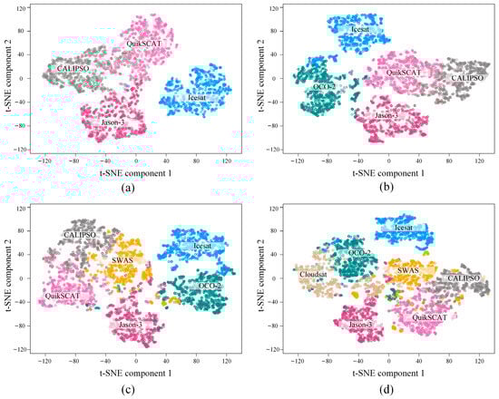
Figure 5.
Visualization of the embedding vectors of different tasks in the scaled scenario. (a–d) Tasks 1–4.
3.4. Model Comparisons
The average accuracy of several incremental learning models is compared with MMFAN in Table 4. The joint train refers to training all task data simultaneously on Mix-Mamba, which is the theoretical upper bound performance of the backbone network. ICaRL [13] is a data replay model, MEMO [46] and FOSTER [47] are dynamic structure models, and BiC [53] is based on model regularization. The backbone of these models is ResNet32, and the exemplar number is set to 20 for each task. Moreover, some new non-exemplar incremental learning models like FeTrIL [19], DS-AL [57], and ACIL [67] are also compared.
Table 4.
Mean accuracy and confidence comparisons of different incremental learning models.
It can be seen that the proposed MMFAN achieves higher average accuracy in all test scenarios. Compared to exemplar-based models, although without original data, non-exemplar models can still avoid catastrophic forgetting through special network parameters or feature transfer techniques. Nevertheless, non-exemplar models also have significant advantages in terms of data storage and security. The accuracy evolution with incremental tasks of these models is shown in Figure 6. As new tasks are added, MMFAN has a lower decay in classification accuracy compared with other methods; therefore, the proposed method maintains better performance during incremental target samples.
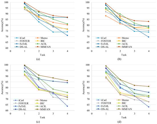
Figure 6.
Accuracy evolution with incremental tasks on different scenarios. (a) Normal scenario. (b) Scaled scenario. (c) Rotated scenario. (d) Combined scenario.
3.5. Ablation Study
To verify the effectiveness modules in MMFAN, an ablation study is conducted on the ISAR image dataset. Specifically, the baseline model is only equipped with a non-exemplar knowledge distillation technique by employing the output of the old model to guide the training of the new model. The backbone of the baseline is Res-Net32 with 20.86 M parameters, and the proposed Mix-Mamba backbone has comparable 21.28 M parameters. In the ablation study, we change the corresponding modules of the baseline with the CST, Mamba vision block, and FAN, respectively, to demonstrate the contribution of these modules. The results of the ablation study in four test scenarios are shown in Table 5, where ‘√’ indicates the inclusion of the corresponding module. It can be seen that CST effectively adjusts the deformation of ISAR images and improves the average accuracy by 3.72%, 5.76%, and 9.5% in the scaled, rotated, and combined test scenarios, respectively, thereby effectively reducing the impact of unknown target deformations on classification. Mamba vision block and FAN enhance network performance by extracting global context features and fine-tuning the features. The combination of these modules can achieve higher accuracy in class-incremental learning.
Table 5.
Results of ablation study on different scenarios.
3.6. Real-World Data Experiments
To validate the incremental classification performance of MMFAN on real-world data, in this section, an eight-class aircraft target ISAR dataset is constructed. Specifically, as shown in Table 6, the first five targets (F15C, F16, F18, F117, and MiG29) are generated through electromagnetic simulation and serve as Task 1, and the imaging configurations are aligned with the normal test scenario introduced in Section 3.1. The remaining three targets (An-6, Citation, and Yak-42) are real-world measured data and serve as Tasks 2–4. The measured ISAR data [68] are obtained using a C-band radar system operating at the center frequency of 5520 MHz, transmitting a linear frequency-modulated (LFM) chirp signal with a 400 MHz bandwidth and 400 Hz pulse repetition frequency (PRF). Post-dechirp sampling is performed at 10 MHz. Three aircraft types are involved: the An-26 is a medium-sized turboprop aircraft, the Citation is a small business jet plane, and the Yak-42 is a large regional jetliner. Figure 7 illustrates the ground-projected trajectories of these aircraft relative to the radar origin (0,0), enabling approximate azimuth angle estimation. The optical images and ISAR image examples for each target are shown in Figure 8.
Table 6.
Incremental learning task configurations of the real-world dataset.
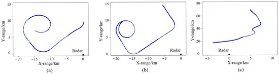
Figure 7.
Projections of target trajectories onto the ground. (a) An-26. (b) Citation. (c) Yak-42.
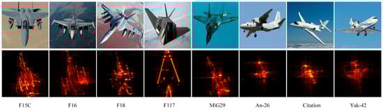
Figure 8.
Optical and typical ISAR image samples of the aircraft targets.
To explore the differences in distribution between the simulated data (Targets 1–5) and the measured data (Targets 6–8), the statistical histogram of mean pixel-level intensity is show in Figure 9a. After quantitative domain-shift analysis, the simulated images exhibit a smaller mean value (5.01) and inter-image standard deviation (+2.19) than the measured images, indicating cleaner backgrounds in simulated data with fewer imaging fluctuations caused by target movements. In the feature space, we also analyze the distribution differences between simulated and measured data through kernel mapping and PCA dimensionality reduction. As shown in Figure 9b, the simulated and measured feature distributions illustrate distinct separations, with a Wasserstein distance of 1.28 and a Jensen–Shannon divergence of 0.6. Moreover, the distances between categories in measured data are also larger than those in simulated data.
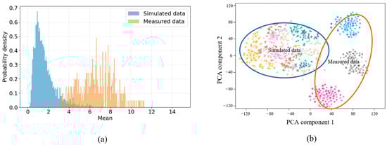
Figure 9.
Domain-shift analyses of simulated data and measured data. (a) Histogram of the mean pixel values. (b) Feature space distribution through PCA dimensionality reduction.
The accuracy comparisons with existing methods on real-world data are presented in Table 7, and the accuracy evolution across tasks is illustrated in Figure 10. The real-world measured data differs from simulated data in radar parameters and imaging configurations, introducing heightened incremental learning challenges. Despite this, MMFAN still demonstrates better performance in real-world scenarios and achieves an average classification accuracy of 87.5%.
Table 7.
Mean accuracy and confidence comparisons of different models with real-world dataset.
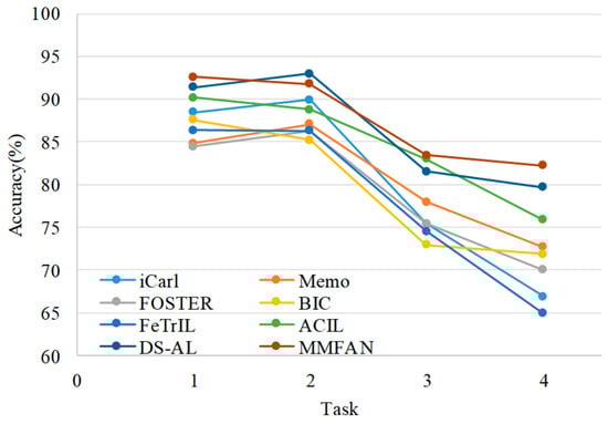
Figure 10.
Accuracy evolution with incremental tasks on real-world data.
3.7. Learning from Scratch
In real-world classification tasks, the initial training data are often extremely limited, and the target type retrieved by radar varies greatly each time. This highlights the adaptability of the model to data variations and memory for old tasks. To verify the performance of MMFAN in learning from scratch, in this section, the 12-task incremental learning-from-scratch dataset is constructed as shown in Table 8. Among them, the first seven tasks learn from the seven satellite targets in Section 3.1 one by one, while the last five tasks learn from five airplane targets (F15C, F16, F18, F117, and MiG29) in Section 3.6.
Table 8.
Task configurations of incremental learning from scratch.
The learning-from-scratch comparison of existing models and MMFAN is shown in Table 9. It can be seen that learning from scratch requires more complex historical information, and the accuracy of all models is decreased compared with the result of learning from the middle in Table 6. For example, in the combined scenario, DS-AL suffers with a 10.69% drop in accuracy, while MMFAN only drops by 4.86% because of the stronger incremental stability. The accuracy evolution of these models learning from scratch on four test scenarios is shown in Figure 11. As the number of incremental tasks further increases, MMFAN is able to maintain a classification performance advantage, particularly in the combined test scenario. Specifically, the increased accuracy in Task 8 is because of the data variation between satellite targets and aircraft targets. The feature distribution of Task 8 is stronger than that of the first seven tasks, so the accuracy is higher than that of Task 7.
Table 9.
Mean accuracy and confidence comparisons of different models with learning from scratch.
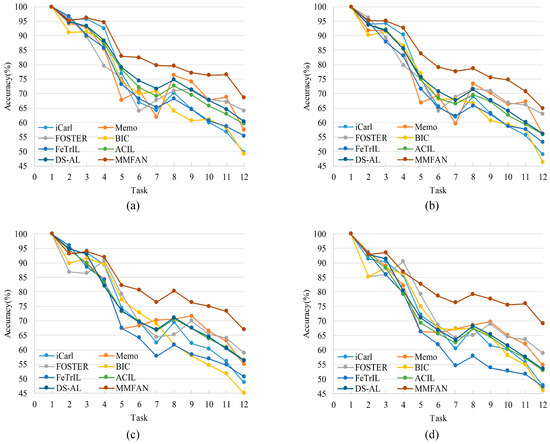
Figure 11.
Accuracy evolution with learning from scratch on different scenarios. (a) Normal scenario. (b) Scaled scenario. (c) Rotated scenario. (d) Combined scenario.
4. Discussion
With the rapid advancement of deep learning, numerous high-precision networks have been proposed for target classification. However, training networks on radar images with unknown deformation distortions while accommodating continuously emerging targets has drawn significant attention. In this article, a non-exemplar class-incremental learning method, MMFAN, is proposed, which effectively learns new task data while preserving historical knowledge of previous tasks. In the incremental learning experiments, the effectiveness of the proposed method is evaluated through accuracy, a confusion matrix, and t-SNE visualization. Experimental results demonstrate that MMFAN achieves superior average accuracy compared to exemplar-based benchmarks (iCarl, Memo, FOSTER, and BIC) and outperforms recent non-exemplar approaches. The confusion matrix reveals the retention of prior knowledge, while feature visualization illustrates how the FAN dynamically adjusts prototypes and feature distributions to minimize intra-class variance and mitigate catastrophic forgetting. Notably, MMFAN exhibits optimal performance across scaled, rotated, and combined deformation scenarios. Ablation studies further elucidate the contributions of each component: CST enhances deformation robustness, Mamba vision blocks establish baseline performance improvements, and the FAN drives incremental learning efficacy. The synergistic integration of these modules yields better overall performance, confirming the advantages of MMFAN in ISAR incremental learning. In addition, experiments that are closer to practical applications are conducted, including real-world data and a learning-from-scratch paradigm. The real-world ISAR data is more blurred and noisier, and learning-from-scratch will face greater data variations and memory challenges. The experimental results further validate the sustained classification accuracy of MMFAN.
Despite these promising results, MMFAN presents limitations, including higher computational demands from Mamba Vision compared to convolutional architectures and the complexity of loss function design, requiring precise parameter tuning. Future work will also prioritize developing few-shot incremental learning frameworks for ISAR target classification under extreme sample scarcity, alongside multi-modal data fusion architectures for aerospace target recognition.
5. Conclusions
To address the challenges of catastrophic forgetting and unknown image deformations in incremental ISAR target classification, this article proposes MMFAN, a non-exemplar class-incremental learning method. Specifically, the Mix-Mamba backbone performs image deformation adjustment using CST and obtains global feature representation through Mamba vision blocks. FAN manages and transfers these features adaptively across different tasks. The loss bar integrates knowledge distillation, feature replay losses, and supervised and unsupervised losses to facilitate the network training. Experimental results on the ISAR datasets demonstrate the effectiveness of MMFAN in improving incremental classification accuracy while maintaining deformation robustness across various test scenarios.
Author Contributions
Conceptualization, R.X. and C.L.; methodology, R.X.; software, R.X.; validation, R.X. and W.P.; formal analysis, W.P.; investigation, R.X.; resources, X.B.; data curation, X.B.; writing—original draft preparation, R.X.; writing—review and editing, X.B. and F.Z.; visualization, R.X.; supervision, C.L. and X.B.; project administration, C.L.; funding acquisition, C.L. All authors have read and agreed to the published version of the manuscript.
Funding
This research was funded in part by the National Key Research and Development Program of China under Grant 2022YFB3902404 and in part by the National Natural Science Foundation of China under Grant 62401464 and Grant 62301417.
Data Availability Statement
The original contributions presented in the study are included in the article, further inquiries can be directed to the corresponding author.
Acknowledgments
The authors would like to thank all anonymous reviewers and editors for their useful comments and suggestions, which greatly improved this article.
Conflicts of Interest
The authors declare no conflicts of interest.
References
- Rosenberg, L.; Zhao, W.; Heng, A.; Hamey, L.; Nguyen, S.T.; Orgun, M.A. Classification of ISAR ship imagery using transfer learning. IEEE Trans. Aerosp. Electron. Syst. 2024, 60, 25–36. [Google Scholar] [CrossRef]
- Shao, S.; Liu, H.; Wei, J. GEO targets ISAR imaging with joint intra-pulse and inter-pulse high-order motion compensation and sub-aperture image fusion at ULCPI. IEEE Trans. Geosci. Remote Sens. 2024, 62, 5200515. [Google Scholar] [CrossRef]
- Wu, D.-M.; Kiang, J.-F. Imaging of high-speed aerial targets with ISAR installed on a moving vessel. IEEE J. Sel. Topics Appl. Earth Observ. Remote Sens. 2023, 16, 6463–6474. [Google Scholar] [CrossRef]
- Yuan, H.; Li, H.; Zhang, Y.; Li, M.; Wei, C. Few-Shot Classification for ISAR Images of Space Targets by Complex-Valued Patch Graph Transformer. IEEE Trans. Aerosp. Electron. Syst. 2024, 60, 4896–4909. [Google Scholar] [CrossRef]
- Dong, G.; Liu, H. Target recognition in ISAR image via range profile perturbation imaging. IEEE Trans. Geosci. Remote Sens. 2024, 62, 5227811. [Google Scholar] [CrossRef]
- Du, H.; Ni, P.; Chen, J.; Ma, S.; Zhang, H.; Xu, G. Integrated convolution network for ISAR imaging and target recognition. IEEE J. Miniaturization Air Space Syst. 2023, 4, 431–437. [Google Scholar] [CrossRef]
- Bai, X.; Yang, M.; Chen, B.; Zhou, F. REMI: Few-shot ISAR target classification via robust embedding and manifold inference. IEEE Trans. Neural Netw. Learn. Syst. 2025, 34, 6000–6013. [Google Scholar] [CrossRef]
- Duan, J.; Ma, Y.; Zhang, L.; Xie, P. Abnormal dynamic recognition of space targets from ISAR image sequences with SSAE-LSTM Network. IEEE Trans. Geosci. Remote Sens. 2023, 61, 5102916. [Google Scholar] [CrossRef]
- Zhang, Y.; Bai, X.; Liu, S.; Zhou, F. Joint translational motion compensation and high-resolution ISAR imaging based on sparse bayesian learning. IEEE Trans. Comput. Imaging 2024, 12, 1–10. [Google Scholar] [CrossRef]
- Santi, F.; Pisciottano, I.; Cristallini, D.; Pastina, D. Impact of rotational motion estimation errors on passive bistatic ISAR imaging via backprojection algorithm. IEEE J. Sel. Topics Appl. Earth Observ. Remote Sens. 2024, 17, 3345–3365. [Google Scholar] [CrossRef]
- Chen, C.; Tian, S.; Xu, Z. ISAR imaging for maneuvering targets via fast rotation parameter estimation. IEEE Geosci. Remote Sens. Lett. 2023, 20, 3505105. [Google Scholar] [CrossRef]
- Zhou, D.; Wang, Q.; Qi, Z.; Ye, H.; Zhan, D.; Liu, Z. Class-incremental learning: A survey. IEEE Trans. Pattern Anal. Mach. Intell. 2024, 46, 9851–9873. [Google Scholar] [CrossRef] [PubMed]
- Refbuffi, S.-A.; Kolesnikov, A.; Sperl, G.; Lampert, C.H. iCaRL: Incremental classifier and representation learning. In Proceedings of the IEEE Conference Computer Vision and Pattern Recognition (CVPR), Honolulu, HI, USA, 21–26 July 2017; pp. 2001–2010. [Google Scholar] [CrossRef]
- Korycki, L.; Krawczyk, B. Class-incremental experience replay for continual learning under concept drift. In Proceedings of the IEEE/CVF Conference Computer Vision Pattern Recognition Workshops (CVPRW), Nashville, TN, USA, 19–25 June 2021; pp. 3644–3653. [Google Scholar] [CrossRef]
- Shin, H.; Lee, J.K.; Kim, J.; Kim, J. Continual learning with deep generative replay. In Proceedings of the International Conference Neural Information Processing Systems, Long Beach, CA, USA, 4–9 December 2017; pp. 2990–2999. [Google Scholar]
- Zhang, H.; Sindagi, V.; Patel, V.M. Image de-raining using a conditional generative adversarial network. IEEE Trans. Circuits Syst. Video Technol. 2020, 30, 3943–3956. [Google Scholar] [CrossRef]
- Gao, R.; Liu, W. DDGR: Continual learning with deep diffusion-based generative replay. In Proceedings of the International Conference on Machine Learning (ICML), Honolulu, HI, USA, 23–29 July 2023; pp. 10744–10763. [Google Scholar]
- Shi, W.; Ye, M. Prototype reminiscence and augmented asymmetric knowledge aggregation for non-exemplar class-incremental learning. In Proceedings of the International Conference Computer Vision (ICCV), Paris, France, 2–6 October 2023; pp. 1772–1781. [Google Scholar] [CrossRef]
- Petit, G.; Popescu, A.; Schindler, H.; Picard, D.; Delezoide, B. FeTrIL: Feature translation for exemplar-free class-incremental learning. In Proceedings of the IEEE/CVF Winter Conference Applications Computer Vision (WACV), Waikoloa, HI, USA, 2–7 January 2023; pp. 3900–3909. [Google Scholar] [CrossRef]
- Musman, S.; Kerr, D.; Bachmann, C. Automatic recognition of ISAR ship images. IEEE Trans. Aerosp. Electron. Syst. 1996, 32, 1392–1404. [Google Scholar] [CrossRef]
- Benedek, C.; Martorella, M. Moving target analysis in ISAR image sequences with a multiframe marked point process model. IEEE Trans. Geosci. Remote Sens. 2014, 52, 2234–2246. [Google Scholar] [CrossRef]
- Lee, S.J.; Lee, M.J.; Bae, J.H.; Kim, K.T. Classification of ISAR images using variable cross-range resolutions. IEEE Trans. Aerosp. Electron. Syst. 2018, 54, 2291–2303. [Google Scholar] [CrossRef]
- Paladini, R.; Martorella, M.; Berizzi, F. Classification of man-made targets via invariant coherency-matrix eigenvector decomposition of polarimetric SAR/ISAR images. IEEE Trans. Geosci. Remote Sens. 2011, 49, 3022–3034. [Google Scholar] [CrossRef]
- Kondaveeti, H.K.; Vatsavayi, V.K. Abridged shape matrix representation for the recognition of aircraft targets from 2D ISAR imagery. Adv. Comput. Sci. Technol. 2017, 10, 1103–1122. [Google Scholar] [CrossRef]
- Park, S.H.; Jung, J.H.; Kim, S.H.; Kim, K.T. Efficient classification of ISAR images using 2D Fourier transform and polar mapping. IEEE Trans. Aerosp. Electron. Syst. 2015, 51, 1726–1736. [Google Scholar] [CrossRef]
- Lee, S.J.; Park, S.H.; Kim, K.T. Improved classification performance using ISAR images and trace transform. IEEE Trans. Aerosp. Electron. Syst. 2017, 53, 950–965. [Google Scholar] [CrossRef]
- Xu, G.; Xing, M.; Xia, X.; Zhang, L.; Chen, Q.; Bao, Z. 3D geometry and motion estimations of maneuvering targets for interferometric ISAR with sparse aperture. IEEE Trans. Image Process. 2016, 25, 2005–2020. [Google Scholar] [CrossRef] [PubMed]
- Deng, J.; Xie, P.; Zhang, L.; Cong, Y. ISAR-NeRF: Neural radiance fields for 3-D imaging of space target from multiview ISAR images. IEEE Sens. J. 2024, 24, 11705–11722. [Google Scholar] [CrossRef]
- Li, X.; Ran, J.; Wen, Y.; Wei, S.; Yang, W. MVFRnet: A novel highaccuracy network for ISAR air-target recognition via multi-view fusion. Remote Sens. 2023, 15, 3052. [Google Scholar] [CrossRef]
- Yuan, H.; Li, H.; Zhang, Y.; Wei, C.; Gao, R. Complex-valued multiscale vision transformer on space target recognition by ISAR image sequence. IEEE Geosci. Remote Sens. Lett. 2024, 21, 4008305. [Google Scholar] [CrossRef]
- Edelman, B.L.; Goel, S.; Kakade, S.; Zhang, C. Inductive biases and variable creation in self-attention mechanisms. In Proceedings of the International Conference on Machine Learning (ICML), Baltimore, MD, USA, 17–23 July 2022; pp. 5793–5831. [Google Scholar]
- Sun, Y.; Dong, L.; Huang, S.; Ma, S.; Xia, Y.; Xue, J.; Wang, J.; Wei, F. Retentive network: A successor to Transformer for large language models. arXiv 2023, arXiv:2307.08621. [Google Scholar]
- Gu, A.; Goel, K.; Ré, C. Efficiently modeling long sequences with structured state spaces. arXiv 2021, arXiv:2111.00396. [Google Scholar]
- Gu, A.; Goel, K.; Gupta, A.; Ré, C. On the parameterization and initialization of diagonal state space models. In Proceedings of the Advances in Neural Information Processing Systems, New Orleans, LA, USA, 28 November–9 December 2022; pp. 35971–35983. [Google Scholar]
- Zhang, H.; Zhu, Y.; Wang, D.; Zhang, L.; Chen, T.; Wang, Z.; Ye, Z. A Survey on Visual Mamba. Appl. Sci. 2024, 14, 5683. [Google Scholar] [CrossRef]
- Zhu, L.; Liao, B.L.; Zhang, Q.; Wang, X.; Liu, W.; Wang, X. Vision mamba: Efficient visual representation learning with bidirectional state space model. In Proceedings of the 41st International Conference on Machine Learning (ICML), Vienna, Austria, 21–27 July 2024; pp. 62429–62442. Available online: https://proceedings.mlr.press/v235/zhu24f.html (accessed on 9 May 2025).
- Yang, H.; Zhang, Y.; Ding, W. Multiple heterogeneous P-DCNNs ensemble with stacking algorithm: A novel recognition method of space target ISAR images under the condition of small sample set. IEEE Access 2020, 8, 75543–75570. [Google Scholar] [CrossRef]
- Ni, P.; Liu, Y.; Pei, H.; Du, H.; Li, H.; Xu, G. CLISAR-Net: A deformation-robust ISAR image classification network using contrastive learning. Remote Sens. 2022, 15, 33. [Google Scholar] [CrossRef]
- Bai, X.; Zhou, X.; Zhang, F.; Wang, L.; Xue, R.; Zhou, F. Robust Pol-ISAR target recognition based on ST-MC-DCNN. IEEE Trans. Geosci. Remote Sens. 2019, 57, 9912–9927. [Google Scholar] [CrossRef]
- Finnveden, L.; Jansson, Y.; Lindeberg, T. Understanding when spatial transformer networks do not support invariance and what to do about it. In Proceedings of the 25th IEEE International Conference on Pattern Recognition (ICPR), Milan, Italy, 10–15 January 2021; pp. 3427–3434. [Google Scholar] [CrossRef]
- Zhao, Y.; Zhao, L.; Ding, D.; Hu, D.; Kuang, G.; Liu, L. Few-shot class-incremental SAR target recognition via orthogonal distributed features. IEEE Trans. Aerosp. Electron. Syst. 2025, 61, 325–341. [Google Scholar] [CrossRef]
- Li, Y.; Du, L.; Liu, H.; Guo, Y. Class-incremental SAR ship detection and classification via context-robust exemplar replay and multi-granularity knowledge distillation. IEEE Trans. Aerosp. Electron. Syst. 2025, in press. [Google Scholar] [CrossRef]
- Rusu, A.A.; Rabinowitz, N.C.; Desjardins, G.; Soyer, H.; Kirkpatrick, J.; Kavukcuoglu, K.; Pascanu, R.; Hadsell, R. Progressive neural networks. arXiv 2016, arXiv:1606.04671. [Google Scholar]
- Yan, S.; Xie, J.; He, X. DER: Dynamically expandable representation for class incremental learning. In Proceedings of the IEEE/CVF Conference Computer Vision and Pattern Recognition, Nashville, TN, USA, 20–25 June 2021; pp. 3013–3022. [Google Scholar] [CrossRef]
- Liu, Y.; Schiele, B.; Sun, Q. Adaptive aggregation networks for class-incremental learning. In Proceedings of the IEEE/CVF Conference Computer Vision and Pattern Recognition, Nashville, TN, USA, 20–25 June 2021; pp. 2544–2553. [Google Scholar] [CrossRef]
- Zhou, D.-W.; Wang, Q.-W.; Ye, H.-J.; Zhan, D.-C. A model or 603 exemplars: Towards memory-efficient class-incremental learning. arXiv 2022, arXiv:2205.13218. [Google Scholar]
- Wang, F.Y.; Zhou, D.W.; Ye, H.J.; Zhan, D.C. Foster: Feature boosting and compression for class-incremental learning. In Proceedings of the European Conference on Computer Vision, Tel Aviv, Israel, 23–27 October 2022; pp. 398–414. [Google Scholar] [CrossRef]
- Zhu, K.; Zhai, W.; Cao, Y.; Luo, J.; Zha, Z.-J. Self-sustaining representation expansion for non-exemplar class-incremental learning. In Proceedings of the IEEE/CVF Conference on Computer Vision and Pattern Recognition, New Orleans, LA, USA, 18–24 June 2022; pp. 9286–9295. [Google Scholar] [CrossRef]
- Kirkpatrick, J.; Pascanu, R.; Rabinowitz, N.; Veness, J.; Desjardins, G.; Rusu, A.A.; Milan, K.; Quan, J.; Ramalho, T.; Grabska-Barwinska, A.; et al. Overcoming catastrophic forgetting in neural networks. Proc. Nat. Acad. Sci. USA 2017, 114, 3521–3526. [Google Scholar] [CrossRef]
- Zenke, F.; Poole, B.; Ganguli, S. Continual learning through synaptic intelligence. In Proceedings of the International Conference on Machine Learning, Sydney, Australia, 6–11 August 2017; pp. 3987–3995. [Google Scholar]
- Yang, Y.; Zhou, D.-W.; Zhan, D.-C.; Xiong, H.; Jiang, Y.; Yang, J. Cost-effective incremental deep model: Matching model capacity with the least sampling. IEEE Trans. Knowl. Data Eng. 2023, 35, 3575–3588. [Google Scholar] [CrossRef]
- Li, Z.; Hoiem, D. Learning without forgetting. IEEE Trans. Pattern Anal. Mach. Intell. 2018, 40, 2935–2947. [Google Scholar] [CrossRef]
- Wu, Y.; Chen, Y.; Wang, L.; Ye, Y.; Liu, Z.; Guo, Y.; Fu, Y. Large scale incremental learning. In Proceedings of the IEEE/CVF Conference on Computer Vision and Pattern Recognition (CVPR), Long Beach, CA, USA, 15–20 June 2019; pp. 374–382. [Google Scholar] [CrossRef]
- Hou, S.; Pan, X.; Loy, C.C.; Wang, Z.; Lin, D. Learning a unified classifier incrementally via rebalancing. In Proceedings of the IEEE/CVF Conference on Computer Vision and Pattern Recognition (CVPR), Long Beach, CA, USA, 15–20 June 2019; pp. 374–382. [Google Scholar] [CrossRef]
- Douillard, A.; Cord, M.; Ollion, C.; Robert, T.; Valle, E. PODNet: Pooled outputs distillation for small-tasks incremental learning. In Proceedings of the IEEE/CVF Conference on Computer Vision and Pattern Recognition, Glasgow, UK, 23–28 August 2020; pp. 86–102. [Google Scholar] [CrossRef]
- Dhar, P.; Singh, R.V.; Peng, K.-C.; Wu, Z.; Chellappa, R. Learning without memorizing. In Proceedings of the IEEE/CVF Conference on Computer Vision and Pattern Recognition, Long Beach, CA, USA, 15–20 June 2019; pp. 5133–5141. [Google Scholar] [CrossRef]
- Zhuang, H.; He, R.; Tong, K.; Zeng, Z.; Chen, C.; Lin, Z. DS-AL: A dual-stream analytic learning for exemplar-free class-incremental learning. In Proceedings of the AAAI Conference on Artificial Intelligence, Vancouver, BC, Canada, 20–27 February 2024; pp. 17237–17244. [Google Scholar] [CrossRef]
- Li, B.; Cui, Z.; Wang, H.; Deng, Y.; Ma, J.; Yang, J.; Cao, Z. SAR incremental automatic target recognition based on mutual information maximization. IEEE Geosci. Remote Sens. Lett. 2024, 21, 4005305. [Google Scholar] [CrossRef]
- Gu, A.; Dao, T. Mamba: Linear-time sequence modeling with selective state spaces. arXiv 2023, arXiv:2312.00752. [Google Scholar]
- Xue, R.; Bai, X.; Yang, M.; Chen, B.; Zhou, F. Feature distribution transfer learning for robust few-shot ISAR space target recognition. IEEE Trans. Aerosp. Electron. Syst. 2024, 60, 9129–9142. [Google Scholar] [CrossRef]
- Hatamizadeh, A.; Kautz, J. Mambavision: A hybrid mamba transformer vision backbone. arXiv 2024, arXiv:2407.08083. [Google Scholar]
- Gu, A.; Johnson, I.; Goel, K.; Saab, K.; Dao, T.; Rudra, A.; Ré, C. Combining recurrent convolutional and continuous-time models with linear state space layers. In Proceedings of the Advances in Neural Information Processing Systems, Red Hook, NY, USA, 7–10 December 2021; pp. 572–585. [Google Scholar]
- Li, Q.; Peng, Y.; Zhou, J. FCS: Feature calibration and separation for non-exemplar class incremental learning. In Proceedings of the IEEE/CVF Conference on Computer Vision and Pattern Recognition, Seattle, WA, USA, 16–22 June 2024; pp. 28495–28504. [Google Scholar] [CrossRef]
- Lou, Y.; Lin, H.; Chen, Q.; Xing, M.; Zhou, S.; Sun, G.-C. 2-D autofocus for high-squint SAR based on affine coordinate back-projection algorithm. IEEE Trans. Geosci. Remote Sens. 2024, 62, 5228217. [Google Scholar] [CrossRef]
- You, Y.; Gitman, I.; Ginsburg, B. Large batch optimization for deep learning: Training BERT in 76 minutes. arXiv 2019, arXiv:1904.00962. [Google Scholar]
- Maaten, L.; Hinton, G. Visualizing data using t-SNE. J. Mach. Learn. Res. 2008, 9, 2579–2605. [Google Scholar]
- Zhuang, H.; Weng, Z.; Wei, H.; Xie, R.; Toh, K.-A.; Lin, Z. ACIL: Analytic class-incremental learning with absolute memorization and privacy protection. In Proceedings of the Advances in Neural Information Processing Systems, New Orleans, LA, USA, 28 November–9 December 2022; pp. 11602–11614. [Google Scholar]
- Du, L.; Liu, H.; Wang, P.; Feng, B.; Pan, M.; Bao, Z. Noise robust radar HRRP target recognition based on multitask factor analysis with small training data size. IEEE Trans. Signal Process. 2012, 60, 3546–3559. [Google Scholar] [CrossRef]
Disclaimer/Publisher’s Note: The statements, opinions and data contained in all publications are solely those of the individual author(s) and contributor(s) and not of MDPI and/or the editor(s). MDPI and/or the editor(s) disclaim responsibility for any injury to people or property resulting from any ideas, methods, instructions or products referred to in the content. |
© 2025 by the authors. Licensee MDPI, Basel, Switzerland. This article is an open access article distributed under the terms and conditions of the Creative Commons Attribution (CC BY) license (https://creativecommons.org/licenses/by/4.0/).