Figure 1.
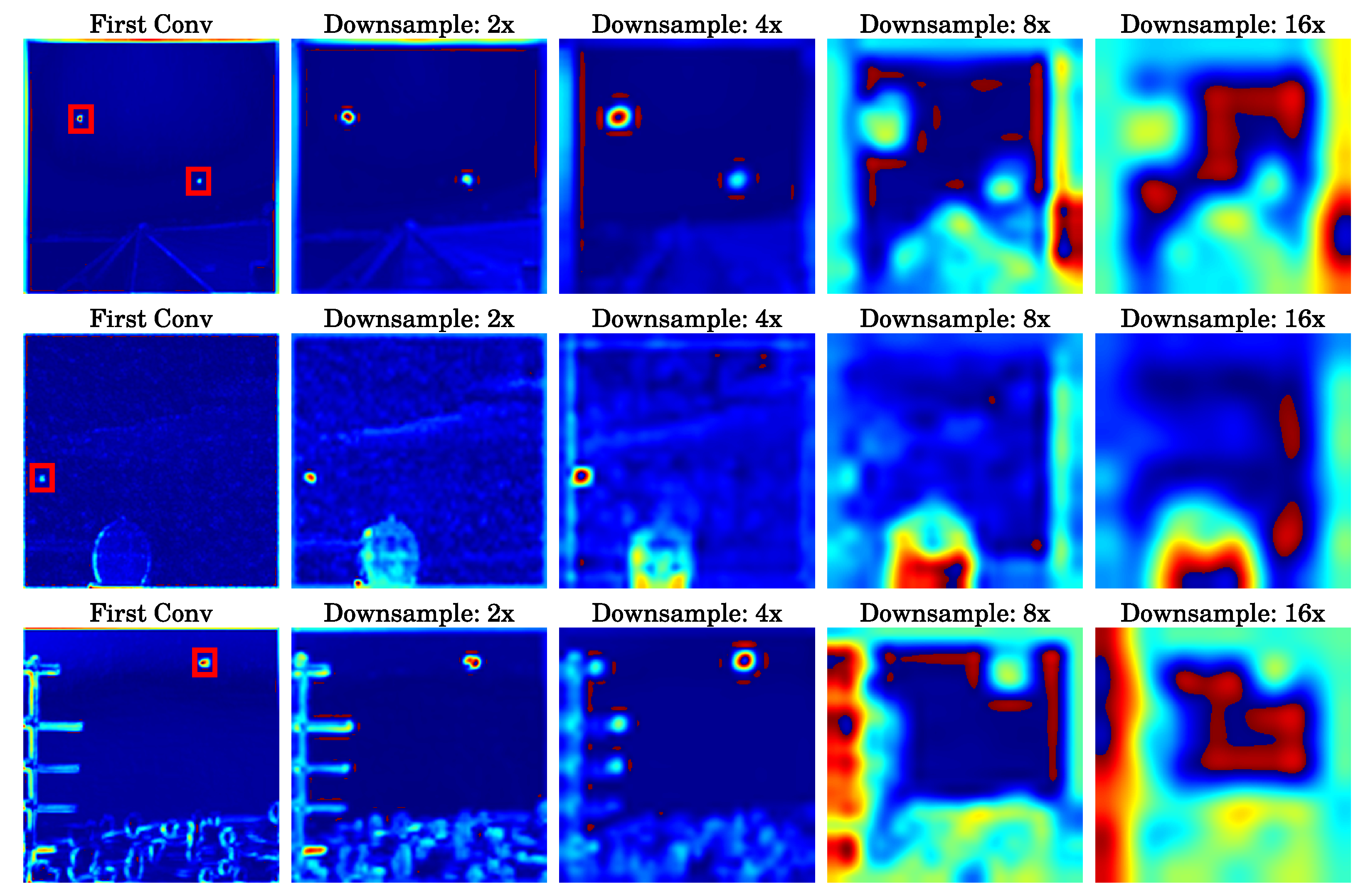
The heatmap distributions of feature maps at different downsampling network layers are presented. In this series of images, the first column shows the result after the network performs its first convolution operation on the input image, with a red box indicating the location of the actual target. The figures sequentially present the analysis results of feature maps at , , , and downsampling ratios. Notably, in the shallow layers of the network where the downsampling ratio is relatively low, the information pertaining to small targets is more prominent.
Figure 1.
The heatmap distributions of feature maps at different downsampling network layers are presented. In this series of images, the first column shows the result after the network performs its first convolution operation on the input image, with a red box indicating the location of the actual target. The figures sequentially present the analysis results of feature maps at , , , and downsampling ratios. Notably, in the shallow layers of the network where the downsampling ratio is relatively low, the information pertaining to small targets is more prominent.
Figure 2.
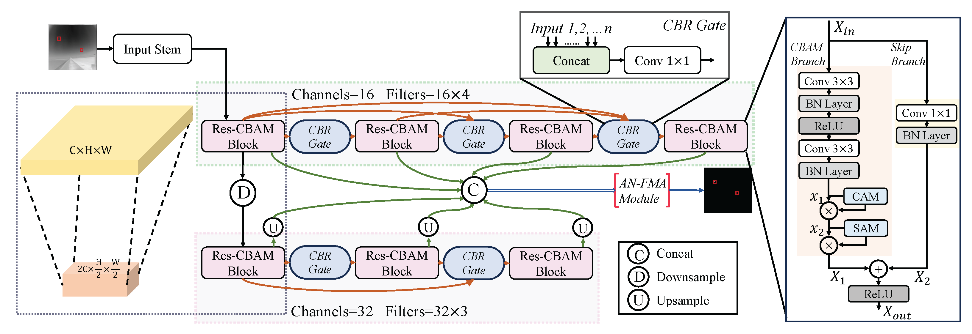
An illustration of the proposed parallel connected lateral chain network (PCLC-Net). The Res-CBAM Block is used for feature extraction, while the CBR Gate plays a role in multi-node feature selection and fusion. The red box in the input image is used to highlight the target area.
Figure 2.
An illustration of the proposed parallel connected lateral chain network (PCLC-Net). The Res-CBAM Block is used for feature extraction, while the CBR Gate plays a role in multi-node feature selection and fusion. The red box in the input image is used to highlight the target area.
Figure 3.
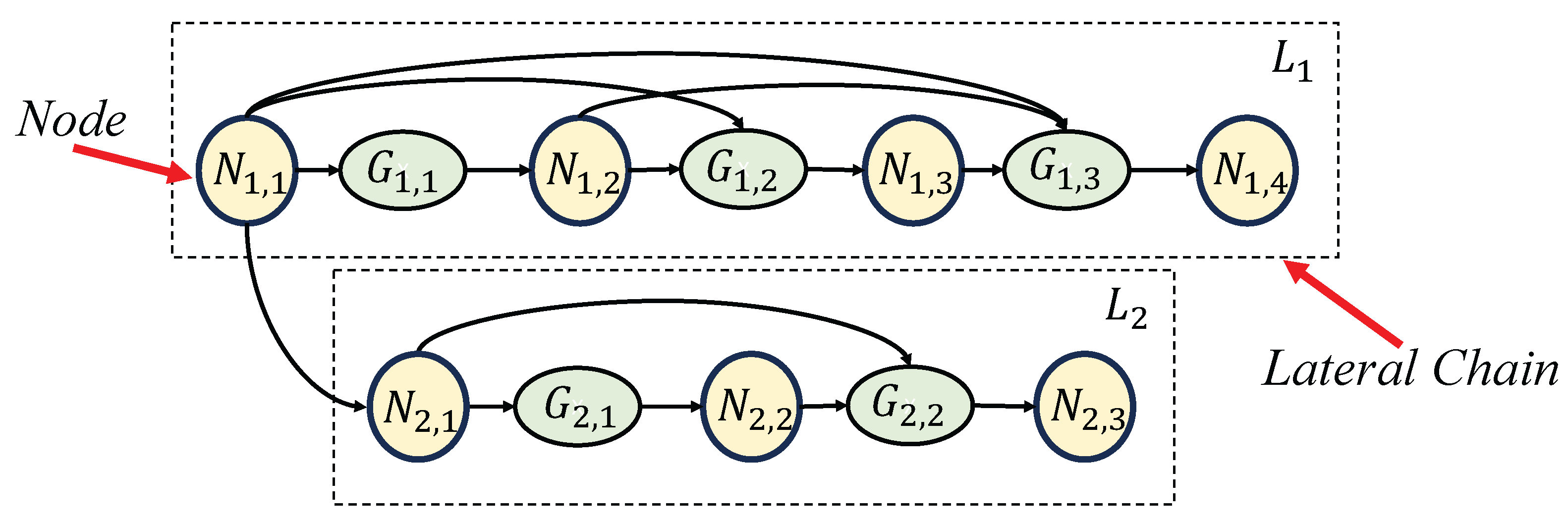
An abstract and simplified network architecture diagram of the PCLC-Net. corresponds to the node of Res-CBAM Block and corresponds to the CBR Gate in the network.
Figure 3.
An abstract and simplified network architecture diagram of the PCLC-Net. corresponds to the node of Res-CBAM Block and corresponds to the CBR Gate in the network.
Figure 4.
Illustration of the AN-FMA module along with its preceding frontend processing. The AN-FMA serves the purpose of integrating the feature maps across all nodes within the network.
Figure 4.
Illustration of the AN-FMA module along with its preceding frontend processing. The AN-FMA serves the purpose of integrating the feature maps across all nodes within the network.
Figure 5.
Quantitative results present the performance of various models on the SIRST dataset. (a) The number of model parameters is plotted along the horizontal axis, while the vertical axis represents the IoU evaluation metric, a crucial indicator of model accuracy. The area of the circular markers is proportional to the model’s FLOPs, visually representing computational complexity. (b) The horizontal axis represents the , while the vertical axis represents the . The area of the octagonal markers signifies the model’s inference speed.
Figure 6.
Quantitative results present the performance of various models on the NUDT-SIRST dataset. (a) The number of model parameters is plotted along the horizontal axis, while the vertical axis represents the IoU evaluation metric, a crucial indicator of model accuracy. The area of the circular markers is proportional to the model’s FLOPs, visually representing computational complexity. (b) The horizontal axis represents the , while the vertical axis represents the . The area of the octagonal markers signifies the model’s inference speed.
Figure 7.
Quantitative results present the performance of various models on the BIT-SIRST dataset. (a) The number of model parameters is plotted along the horizontal axis, while the vertical axis represents the IoU evaluation metric, a crucial indicator of model accuracy. The area of the circular markers is proportional to the model’s FLOPs, visually representing computational complexity. (b) The horizontal axis represents the , while the vertical axis represents the . The area of the octagonal markers signifies the model’s inference speed.
Figure 8.
Qualitative results and 3D visualization results achieved by different SIRST detection methods. The correctly detected target, false alarm, and miss detection areas are highlighted by green, red, and yellow dotted circles, respectively. The area outlined in green indicates the magnified portion for enhanced visualization. Our PCLC-Net can generate output with precise target localization and shape segmentation under a lower false alarm rate.
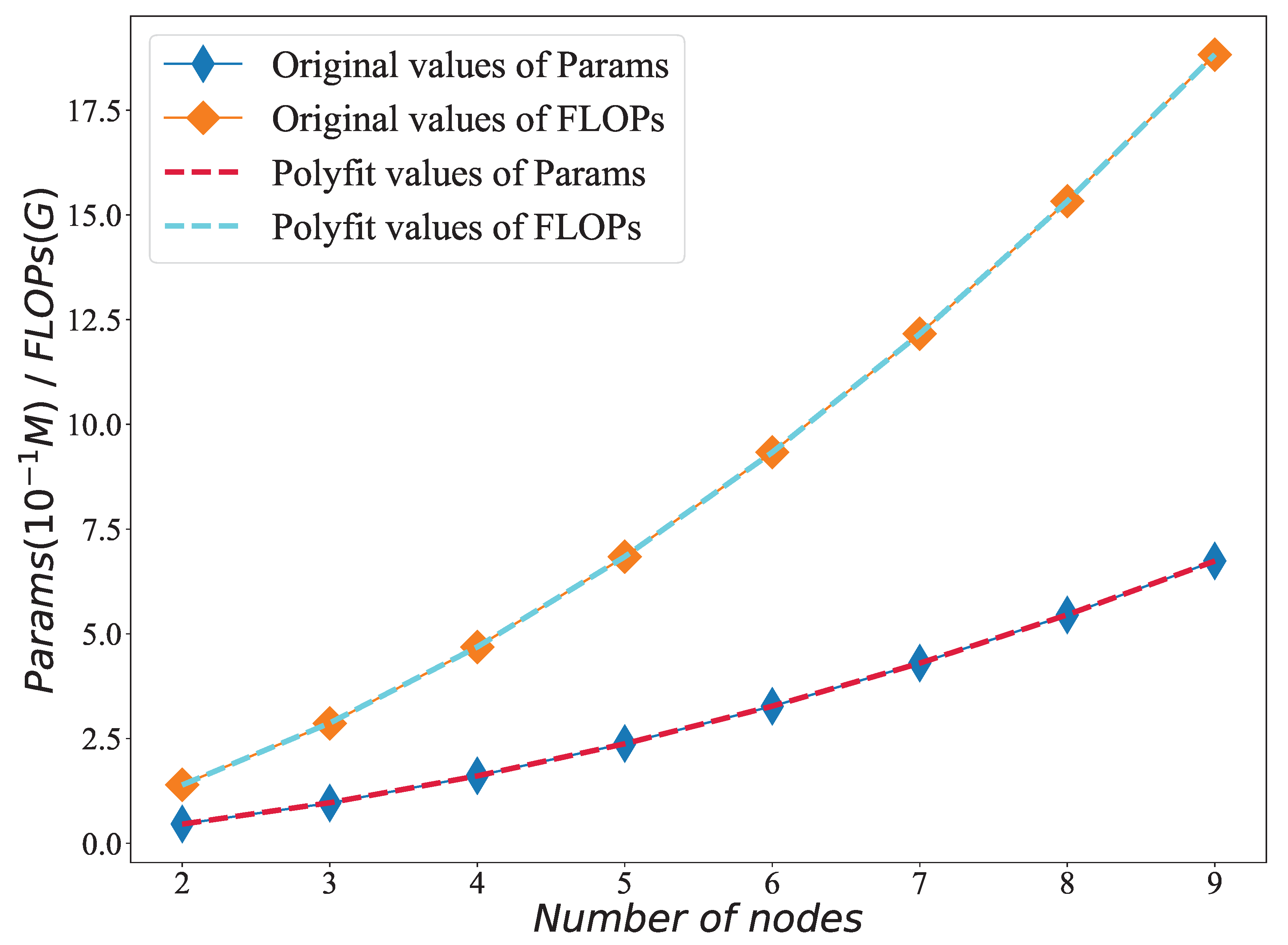
Figure 9.
A diagram depicting the statistical outcomes of network parameter quantities and floating-point operations for varying node counts, accompanied by a quadratic polynomial fitting curve.
Figure 9.
A diagram depicting the statistical outcomes of network parameter quantities and floating-point operations for varying node counts, accompanied by a quadratic polynomial fitting curve.
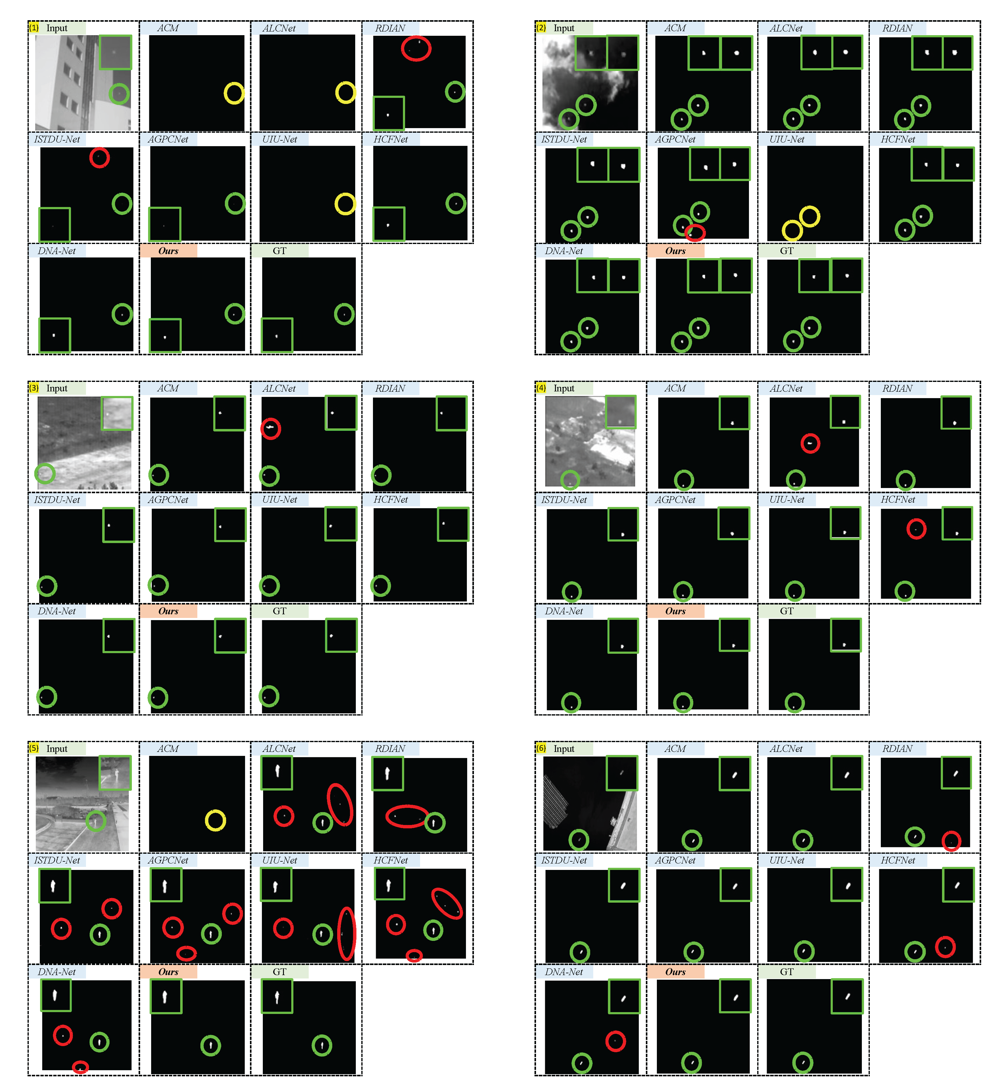
Figure 10.
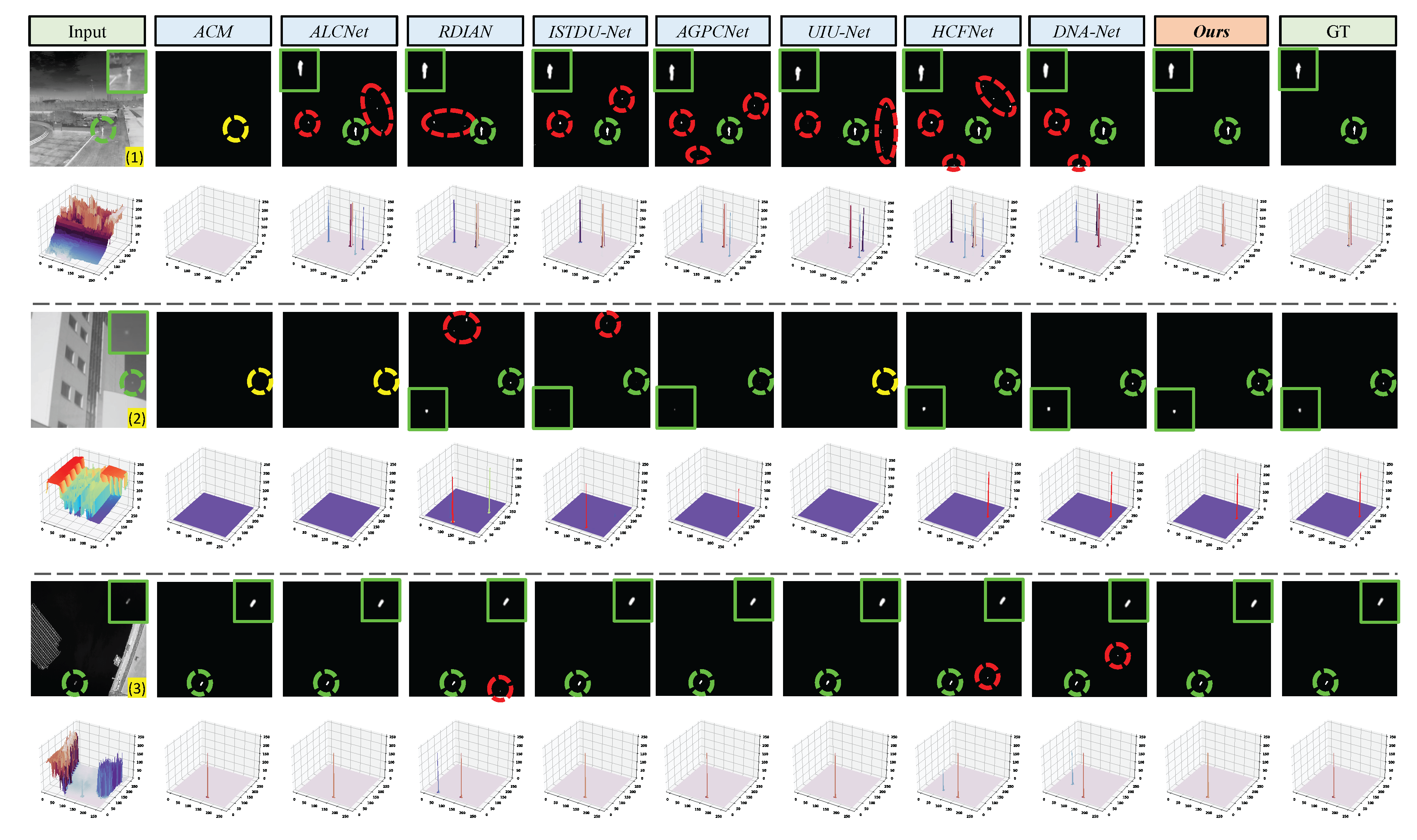
Qualitative results achieved by ACM, ALCNet, RDIAN, ISTDU-Net, AGPCNet, UIU-Net, HCFNet, DNA-Net, and our PCLC-Net (). Green, red, and yellow dotted circles highlight the correctly detected target, false alarm, and miss detection areas, respectively. The area outlined in green indicates the magnified portion for enhanced visualization.
Figure 10.
Qualitative results achieved by ACM, ALCNet, RDIAN, ISTDU-Net, AGPCNet, UIU-Net, HCFNet, DNA-Net, and our PCLC-Net (). Green, red, and yellow dotted circles highlight the correctly detected target, false alarm, and miss detection areas, respectively. The area outlined in green indicates the magnified portion for enhanced visualization.
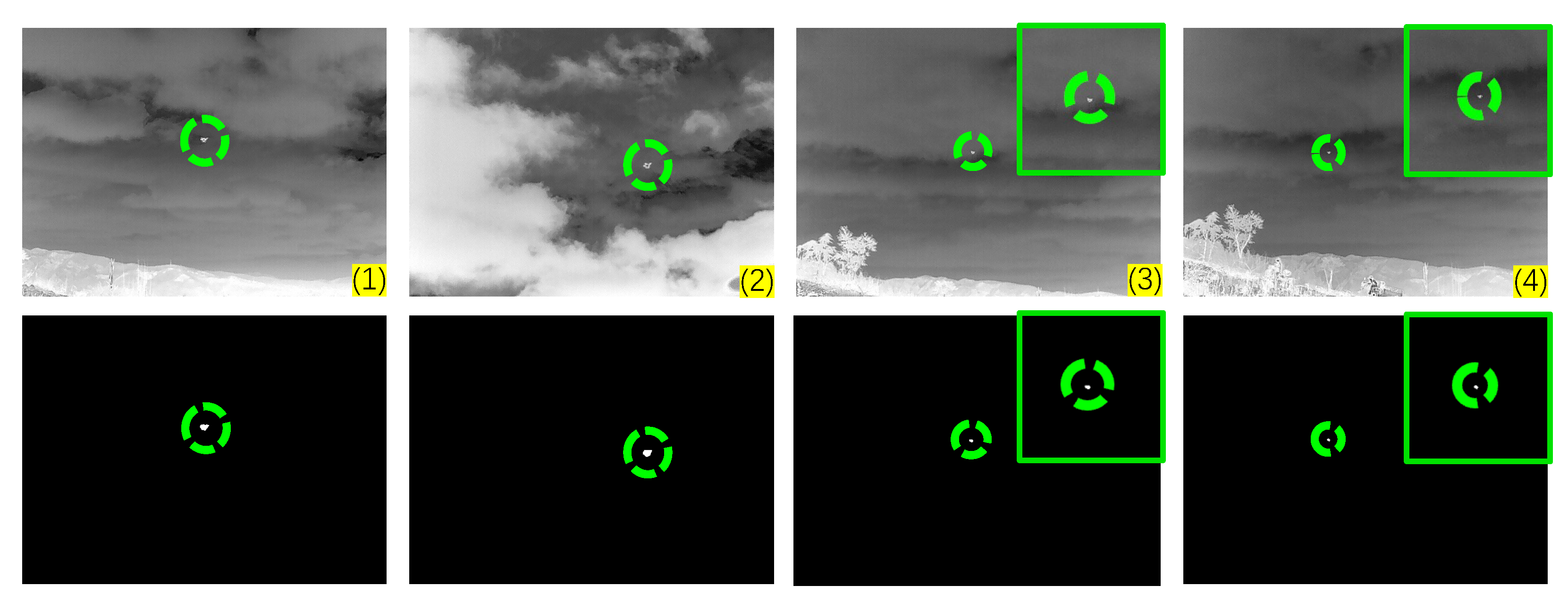
Figure 11.
The 3D visualization results of different methods on 6 test images.
Figure 11.
The 3D visualization results of different methods on 6 test images.
Figure 12.
The visualization results of the PCLC-Net on the custom set. The first row displays the original test images, with the target regions marked by green circles. The second row illustrates the corresponding detection outcomes, where the successfully detected targets are circled in green.
Figure 12.
The visualization results of the PCLC-Net on the custom set. The first row displays the original test images, with the target regions marked by green circles. The second row illustrates the corresponding detection outcomes, where the successfully detected targets are circled in green.
Table 1.
, , and values achieved by different state-of-the-art methods on the SIRST, NUDT-SIRST, and BIT-SIRST datasets. For and , larger values indicate higher performance. For , smaller values indicate higher performance. The best results are underlined.
Table 1.
, , and values achieved by different state-of-the-art methods on the SIRST, NUDT-SIRST, and BIT-SIRST datasets. For and , larger values indicate higher performance. For , smaller values indicate higher performance. The best results are underlined.
| Methods | SIRST [15] | NUDT-SIRST [21] | BIT-SIRST [32] |
|---|
| ↑ | ↑ | ↓ | ↑ | ↑ | ↓ | ↑ | ↑ | ↓ |
|---|
| ACM [15] | 42.7 | 93.1 | 25.0 | 64.9 | 94.4 | 13.6 | 61.7 | 93.1 | 62.1 |
| ALCNet [16] | 43.2 | 91.5 | 18.8 | 68.8 | 97.1 | 27.3 | 65.2 | 93.7 | 72.5 |
| ISTDU-Net [17] | 42.6 | 91.9 | 36.4 | 85.4 | 97.3 | 17.1 | 79.9 | 94.2 | 36.5 |
| RDIAN [37] | 41.5 | 93.5 | 56.4 | 79.1 | 96.3 | 27.4 | 76.4 | 91.6 | 63.7 |
| AGPCNet [18] | 42.5 | 93.8 | 46.9 | 82.9 | 97.8 | 10.9 | 79.0 | 94.7 | 42.1 |
| UIU-Net [19] | - | - | - | 91.2 | 98.1 | 40.1 | 80.8 | 93.7 | 52.9 |
| DNA-Net [21] | 43.9 | 94.2 | 24.0 | 93.2 | 98.0 | 5.0 | 81.3 | 95.1 | 34.6 |
| HCFNet [22] | 43.5 | 94.7 | 15.7 | 90.1 | 98.1 | 32.0 | 78.6 | 94.0 | 52.3 |
| Ours () | 44.0 | 95.8 | 14.8 | 92.9 | 98.1 | 4.33 | 80.8 | 95.1 | 28.6 |
Table 2.
Params, FLOPs, and FPS values achieved by different state-of-the-art methods on the SIRST, NUDT-SIRST, and BIT-SIRST datasets.
Table 2.
Params, FLOPs, and FPS values achieved by different state-of-the-art methods on the SIRST, NUDT-SIRST, and BIT-SIRST datasets.
| Methods | Params (M) ↓ | FLOPs (G) ↓ | FPS ↑ |
|---|
| ACM [15] | 0.40 | 0.40 | 89 |
| ALCNet [16] | 0.43 | 0.38 | 90 |
| ISTDU-Net [17] | 2.75 | 7.94 | 42 |
| RDIAN [37] | 0.22 | 3.72 | 54 |
| AGPCNet [18] | 12.43 | 43.26 | 25 |
| UIU-Net [19] | 50.54 | 54.43 | 22 |
| DNA-Net [21] | 4.70 | 14.26 | 19 |
| HCFNet [22] | 14.40 | 23.24 | 29 |
| Ours () | 0.16 | 4.69 | 55 |
Table 3.
, , , Params(M), and FLOPs(G) values achieved by main variants of the PCLC-Net on the BIT-SIRST dataset.
Table 3.
, , , Params(M), and FLOPs(G) values achieved by main variants of the PCLC-Net on the BIT-SIRST dataset.
| | Res-CBAM | CBR Gate | AN-FMA | ↑ | ↑ | ↓ | Params ↓ | FLOPs ↓ |
|---|
| 4 | 3 | √ | × | × | 71.2 | 91.8 | 93.1 | 0.140 | 3.90 |
| 4 | 3 | √ | √ | × | 77.5 | 93.9 | 53.4 | 0.160 | 4.63 |
| 4 | 3 | √ | × | √ | 76.2 | 92.1 | 48.8 | 0.141 | 3.95 |
| 4 | 3 | × | √ | √ | 78.6 | 92.8 | 30.3 | 0.154 | 4.48 |
| 4 | 3 | √ | √ | √ | 80.8 | 95.1 | 28.6 | 0.161 | 4.69 |
| 4 | 0 | √ | √ | √ | 62.1 | 85.3 | 103 | 0.040 | 2.64 |
| 3 | 2 | √ | √ | √ | 77.9 | 92.9 | 52.0 | 0.096 | 2.86 |
| 5 | 4 | √ | √ | √ | 80.9 | 95.7 | 33.0 | 0.238 | 6.84 |
Table 4.
The performance metrics of the PCLC-Net on 8 datasets. The best results are underlined.
Table 4.
The performance metrics of the PCLC-Net on 8 datasets. The best results are underlined.
| Dataset | Split | PCLC-Net () | DNA-Net |
|---|
| ↑ | ↑ | ↓ | ↑ | ↑ | ↓ |
|---|
| NUST-SIRST [38] | 7:3 | 90.3 | 97.0 | 6.64 | 89.4 | 96.7 | 3.59 |
| SIRST [15] | 1:1 | 44.0 | 95.8 | 14.8 | 43.9 | 94.2 | 24.0 |
| IRSTD-1k [39] | 1:1 | 77.8 | 87.5 | 32.3 | 70.3 | 89.7 | 33.8 |
| SIRST v2 [40] | 1:1 | 67.7 | 95.4 | 32.6 | 69.6 | 93.8 | 28.7 |
| NUDT-SIRST [21] | 1:1 | 92.9 | 98.1 | 4.33 | 93.2 | 98.0 | 5.0 |
| IRDST-real [37] | 1:1 | 74.7 | 95.6 | 1.64 | 70.1 | 96.7 | 1.66 |
| ISTDD [18] | 7:3 | 63.4 | 97.9 | 6.54 | 63.6 | 97.0 | 3.26 |
| BIT-SIRST [32] | 7:3 | 80.8 | 95.1 | 28.6 | 81.3 | 95.1 | 34.6 |
Table 5.
Training times for every 10 epochs, achieved by various state-of-the-art methods, on the SIRST, NUDT-SIRST, and BIT-SIRST datasets.
Table 5.
Training times for every 10 epochs, achieved by various state-of-the-art methods, on the SIRST, NUDT-SIRST, and BIT-SIRST datasets.
| Methods | SIRST [15] | NUDT-SIRST [21] | BIT-SIRST [32] |
|---|
| ACM [15] | 38 s | 43 s | 8 min |
| ALCNet [16] | 36 s | 44 s | 8 min |
| ISTDU-Net [17] | 2 min 2 s | 5 min 11 s | 45 min |
| RDIAN [37] | 52 s | 1 min 45 s | 13 min |
| AGPCNet [18] | 2 min 20 s | 6 min 2 s | 54 min |
| UIU-Net [19] | 4 min 37 s | 11 min 20 s | 160 min |
| DNA-Net [21] | 2 min | 5 min 45 s | 46 min |
| HCFNet [22] | 2 min 38 s | 6 min 45 s | 62 min |
| Ours () | 1 min 27s | 3 min 29s | 28 min |
Table 6.
Evaluation outcomes of network variants of the PCLC-Net across various node quantities on the NUDT-SIRST dataset, and Params and FLOPs values achieved by these variants.
Table 6.
Evaluation outcomes of network variants of the PCLC-Net across various node quantities on the NUDT-SIRST dataset, and Params and FLOPs values achieved by these variants.
| Configure | NUDT-SIRST [15] | Params (M) ↓ | FLOPs (G) ↓ |
|---|
| ↑ | ↑ | ↓ |
|---|
| 83.0 | 93.2 | 27.9 | 0.046 | 1.396 |
| 83.3 | 93.6 | 18.7 | 0.096 | 2.863 |
| 92.9 | 98.1 | 4.33 | 0.161 | 4.685 |
| 90.0 | 98.3 | 18.0 | 0.238 | 6.842 |
| 90.1 | 98.3 | 14.7 | 0.327 | 9.335 |
| 90.8 | 98.9 | 21.1 | 0.430 | 12.163 |
| 91.2 | 98.5 | 7.90 | 0.545 | 15.327 |
| 91.3 | 99.0 | 9.22 | 0.674 | 18.827 |
Table 7.
The outcomes of training and evaluating network models featuring different numbers of lateral chains on the NUDT-SIRST dataset.
Table 7.
The outcomes of training and evaluating network models featuring different numbers of lateral chains on the NUDT-SIRST dataset.
| | NUDT-SIRST [15] | Params (M) ↓ | FLOPs (G) ↓ |
|---|
| | ↑ | ↑ | ↓ |
|---|
| PCLC-Net-4 | 83.9 | 97.6 | 16.3 | 0.040 | 2.638 |
| PCLC-Net-43 | 92.9 | 98.1 | 4.33 | 0.161 | 4.685 |
| PCLC-Net-432 | 90.3 | 99.1 | 23.4 | 0.443 | 5.939 |
| PCLC-Net-4321 | 92.1 | 98.6 | 13.2 | 0.974 | 6.602 |
Table 8.
The model’s network structure parameter settings encompass adjustments to the number of lateral chains and their respective channel counts. In this context, - signifies the absence of a particular chain.
Table 8.
The model’s network structure parameter settings encompass adjustments to the number of lateral chains and their respective channel counts. In this context, - signifies the absence of a particular chain.
| | PCLC-Net-4 | PCLC-Net-43 | PCLC-Net-432 | PCLC-Net-4321 |
|---|
| Chains () | (4, -, -, -) | (4, 3, -, -) | (4, 3, 2, -) | (4, 3, 2, 1) |
| Channels () | (16, -, -, -) | (16, 32, -, -) | (16, 32, 64, -) | (16, 32, 64, 128) |
Table 9.
The performance of the PCLC-Net () on the BIT-SIRST dataset, in terms of , , and , was evaluated by varying the feature map dimensions.
Table 9.
The performance of the PCLC-Net () on the BIT-SIRST dataset, in terms of , , and , was evaluated by varying the feature map dimensions.
| | BIT-SIRST [32] | Computational Complexity |
|---|
| ↑ | ↑ | ↓ |
|---|
| 64 | 64 | 26.6 | 90.3 | 834 | 0.0625 × |
| 128 | 128 | 71.8 | 91.2 | 72.3 | 0.25 × |
| 256 | 256 | 80.8 | 95.1 | 28.6 | 1.0× |
| 512 | 512 | 90.1 | 97.2 | 13.6 | 4.0 × |


