Unraveling the Scale Dependency of SIF-Based Phenology: Amplified Trends and Climate Responses

Abstract

Plant phenology is closely related to plant function, ecosystem services, and climate balance. Solar-induced chlorophyll fluorescence (SIF) offers new perspectives on plant phenology at regional and global scales. However, the effect of SIF products at different scales on phenology extraction is still unclear. Understanding of the mechanisms underlying phenological responses to environmental factors remains incomplete. Therefore, in this study, two phenological metrics for the Start of Growing Season (SOS) and the End of Growing Season (EOS) were extracted from the phenology of deciduous forests in the middle and high latitudes of the Northern Hemisphere, utilizing SIF products at scales of 1 km, 5 km, and 50 km, and applying the Savitzky-Golay filtering method along with the dynamic threshold method. Our results showed that the 1-km resolution SIF had a significant advantage over the 5-km and 50-km resolution SIFs in terms of consistency with the extracted phenology results from the Gross Primary Productivity (GPP) sites, with mean absolute errors (MAEs) of 4.48 and 15.49 days for SOS and EOS, respectively. For the 5-km resolution SIF, the MAEs for the same phenological metrics were 9.2 and 21.07 days. For the 50-km resolution SIF, the MAEs were 58.94 and 42.73 days. Meanwhile, this study analyzed the trends of phenology utilizing the three scales of SIF products and found a general trend of advancement. The coarser spatial resolution of the SIF data made the trend of advancement more obvious. Using SHapley Additive exPlanations (SHAP) analysis, we investigated the phenological responses to environmental factors at different scales. We found that SOS/EOS were mainly regulated by soil and air temperature, whereas the scale effect on this analysis’ results was not significant. This study has implications for optimizing the use of data, understanding ecosystem changes, predicting vegetation dynamics under global change, and developing adaptive management strategies.

1. Introduction

Deciduous forests constitute about 32% of all forests globally [1] and are an important component of the terrestrial carbon sink [2,3,4]. Deciduous forests in the Northern Hemisphere are primarily found in temperate regions, including the eastern United States and southern Canada, Europe, and East Asia. These regions harbor a rich diversity of tree species, such as oaks, maples, birches, and elms, which together form highly diverse ecosystems. Such ecosystems are essential for maintaining biodiversity, regulating climate, and providing ecosystem services. The phenological dynamics of deciduous forests directly influence the net carbon dioxide (CO₂) exchange in their ecosystems. For example, if the length of the growing season increases by one day, the net exchange of CO₂ in the ecosystem theoretically increases by 5.98 $\mathrm{g}\mathrm{C}{\mathrm{m}}^{-2}$ [5]. This shift can have significant implications for annual growth, reproductive success, competitive dynamics, and the geographic distribution of these forests [6,7]. Therefore, an accurate assessment of deciduous forest phenology is essential for understanding the seasonal dynamics of carbon, water, and energy within ecosystems. It also provides insights into how deciduous forests respond to climate change.

Remote sensing technology has demonstrated significant advantages in monitoring vegetation phenology by providing information on vegetation dynamics over a wide coverage area or even globally, which is crucial for accurately understanding and predicting the impacts of climate change on vegetation growth [8]. However, disparities in spatial resolution among vegetation indices can critically impact the accuracy of phenological parameter extraction. For instance, while the Normalized Difference Vegetation Index (NDVI) effectively tracks vegetation coverage dynamics [9,10,11,12], its saturation in high biomass areas and susceptibility to soil background interference in sparse vegetation regions [13] may lead to mixed-pixel effects, thereby introducing scale-dependent biases. The Enhanced Vegetation Index (EVI) and its two-band variant, EVI2, address saturation limitations through algorithmic improvements [14,15,16,17] and exhibit reduced sensitivity to soil variations [18,19], making them integral to global phenology products like MODIS (MCD12Q2) and VIIRS (VNP12Q2) [20,21]. Notably, the sensitivity of these indices to vegetation growth remains constrained by spatial resolution: coarse-resolution pixels may fail to detect subtle phenological shifts in low-biomass regions [13]. These limitations fundamentally underscore the inherent uncertainties of traditional vegetation indices in cross-scale phenological monitoring.

Unlike traditional vegetation indices, solar-induced chlorophyll fluorescence (SIF) serves as a remote sensing indicator derived from the physiological properties of plants. It represents the energy re-emitted as fluorescence by chlorophyll molecules after absorbing light energy during photosynthesis. This indicator not only directly reflects plant photosynthetic activity but also exhibits resistance to some degree of cloud and soil background interference. In addition, SIF is closely related to the utilization of light energy by plants as well as total primary productivity (GPP) [22,23,24]. Given the strong correlation between SIF and vegetation’s physiological status, SIF demonstrates higher sensitivity and reliability than traditional vegetation indices in monitoring phenology [25,26], making it a reliable tool for assessing the impacts of climate change on vegetation growth and monitoring vegetation phenology. Increasingly, various SIF products have been used for phenological metrics extraction, as seen in previous studies exploring vegetation phenology that used SIF products provided by the Greenhouse Gas Observing Satellite (GOSAT) and the Global Ozone Monitoring Experiment-2 (GOME-2) [22,27]. However, the spatial resolution of GOSAT and GOME-2 is low (~40 × 80 km for GOME-2; ~10 km in diameter for GOSAT), and the phenological state reflected by pixels with coarse spatial resolution may not adequately represent the seasonal variations in different vegetation communities because of variations in phenological behaviors [28,29,30,31]. Orbital Carbon Observatory-2 (OCO-2) delivers a SIF product with a higher spatial resolution (~1.3 × 2.2 km), tracking phenology events that closely match GPP-based phenology in forests located in mid- and high-latitude regions [32]. However, the limited spatial coverage of OCO-2 restricts its ability to provide comprehensive phenology tracking across the entire globe. Establishing the relationship between SIF and other remote sensing metrics through machine-learning methods can produce higher-resolution continuous SIF datasets. For example, GOSIF, developed by Li and Xiao, integrates OCO-2 SIF with meteorological data, which offers a spatial resolution of 5 km and performs better in phenological tracking [33,34]. Existing studies confirm that remote sensing observations of surface phenology can be significantly affected by differences in data resolution [30,35,36]. For instance, Gao et al. demonstrated that phenological signal mixing within coarse-resolution pixels can lead to biases in trend quantification [37]. Similarly, Melass et al. highlighted that in regions with strong heterogeneity, factors such as topography, land use, urban heat island effects, or coastal influences can drive significant small-scale phenological variations. These fine-grained details are often lost or obscured in coarse-resolution data due to pixel-averaging effects, further underscoring the irreplaceable value of high spatial resolution data in precisely capturing local phenological signals and bridging the gap between ground observations and regional-scale low-to-medium resolution phenological products [38]. In addition, the phenological conditions tracked by SIF data at different scales are commonly used to detect the temporal trends of phenological metrics, such as SOS and EOS [39]. Zhou et al. [40] explored the phenological trends in the Northern Hemisphere region during 2007–2018 using GOME-2 SIF, GOSIF, and CSIF (with a 5 km spatial resolution), and, for the SOS, the SOS data extracted by the three different scales of SIF showed a consistent trend of significant advancement; for EOS, the EOS data extracted by GOME-2 SIF indicated a non-significant delayed trend, which was inconsistent with the non-significant advancement trend of EOS extracted at other scales. There may be differences in the ecological processes and trends revealed at different spatial scales, and this phenomenon deserves further exploration. However, previous studies have mainly focused on the comparison of different SIF data sources or extraction algorithms, leaving a gap in understanding the differences in SIF for phenology identification and trend detection at spatial scales.

Phenological events result from periodic changes in vegetation induced by the combined influence of various environmental factors, including temperature, precipitation, sunlight, and soil conditions [8,41]. Previous studies have explored the response of phenology extracted from different SIF products to multiple climatic factors. For example, Shi et al. [42] found a strong correlation between spring phenology (SOS) and temperature using GOME-2 SIF data. Liu et al. [43] considered soil temperature and soil moisture in their study using GOSIF data and concluded that soil temperature, rather than air temperature, dominated spring phenology and influenced soil moisture to indirectly affect phenology. Ren et al. used GOSIF and CSIF data and concluded that preseason maximum and minimum air temperatures were the primary drivers of spring phenology advancement; furthermore, fall phenology (EOS) exhibited a positive correlation with preseason precipitation, minimum air temperature, and radiation intensity, while a negative correlation was observed with the preseason maximum air temperature. However, previous studies have generally focused on a few fixed environmental variables, and the response of phenology to climate extracted from SIF data at spatial scales remains inadequately understood. To better evaluate the effect of climatic factors on phenological trends, it is essential to design experiments that evaluate the relative importance of multiple climatic factors at different spatial scales.

Therefore, urgent priorities include elucidating how SIF-derived phenology tracking patterns and mechanisms vary with spatial scale, as well as addressing challenges in accurately characterizing phenology when satellite pixel resolutions differ. This includes analyzing the effects of spatial scale on phenological indicator estimation, trend detection, and response to the environment, and exploring whether phenology detected from the coarse-resolution SIF data is representative of the overall phenology captured by finer-resolution SIF products. In this study, we estimated the SOS and EOS from three different scales of solar-induced chlorophyll fluorescence datasets—1 km, 5 km, and 50 km—for deciduous forests in the middle and high latitudes of the Northern Hemisphere during 2008–2017. The main objectives of the study were to (1) compare the effectiveness of phenology tracking using SIF products at different spatial scales, (2) explore the spatial and temporal patterns of phenological events in deciduous forests in the Northern Hemisphere at different scales, and (3) examine the relative importance of climatic factors on phenological trends at different scales.

2. Data and Methods

2.1. Study Area

The deciduous forest region of the Northern Hemisphere, located at latitudes greater than 30 °N and encompassing parts of Europe, Asia, and North America, is the focus of this study. Main climate types include temperate continental, temperate oceanic, temperate monsoon, and Mediterranean climates.

The study used MODIS land cover data MCD12Q1, which presents yearly distribution maps of global land cover types at a spatial resolution of 500 m. Pixels identified as deciduous forest (including both broadleaf (DBF) and needleleaf (DNF) types) were extracted for the period 2008–2017, according to the International Geosphere-Biosphere Programme (IGBP) classification. To match SIF products at three different scales, the deciduous forest data were resampled to 1-km, 5-km, and 50-km resolutions. During resampling, internal consistency was maintained. If over 50% of the pixels within a given window were identified as deciduous forest, the land cover classification for the central pixel was determined to be deciduous forest. The study area is shown in Figure 1.

2.2. Data

2.2.1. SIF Products

In this study, the 2008–2017 SIF dataset from the GOME-2 satellite, mounted on the MetOp—A platform, is used. The satellite observes daily at specific time points in a sun-synchronous orbit, minimizing the effects of variations in solar zenith angles on SIF measurements. The GOME-2 SIF data mainly stem from the filling of the solar Fraunhofer lines around the 740 nm band [44], which were derived through dimensionality reduction techniques and the inversion of a simplified radiative transfer model, specifically designed to isolate the spectral components of atmospheric absorption, surface reflection, and fluorescence emission. To ensure data quality, cloud-contaminated pixels (cloud fraction ≥20%) were masked, and observations with solar zenith angles >70° were excluded. For this study, we utilized 3-level, grid-averaged data at the global scale (0.5° × 0.5°), with the temporal resolution adjusted to every eight days for consistency with other SIF datasets.

This study uses the 2008–2017 GOSIF (Global OCO-2 SIF) dataset, which features an extensive time span, an appropriate seasonal cycle, and high resolution. GOSIF was developed using a machine-learning algorithm that was trained on data from the Orbiting Carbon Observatory-2 (OCO-2). It utilizes vegetation data from the Moderate Resolution Imaging Spectroradiometer (MODIS) and meteorological reanalysis data as its input variables and has a spatial resolution of 0.05° and a temporal resolution of eight days, spanning from 2001 to the present. GOSIF builds a SIF prediction model through the training of machine-learning algorithms and efficiently predicts SIF data on a global scale [45]. The prediction results are verified with the original SIF observations, demonstrating high accuracy and reliability, and they are widely used in large-scale phenological extraction, assessment of terrestrial ecosystem productivity, and inter-annual changes in vegetation phenology.

In addition to the GOME-2 SIF and GOSIF datasets, the global 1-km resolution SIF 8-day product from 2008–2017 was used in this study. This product was constructed using a similar framework to the GOME-2 SIF, incorporating machine-learning technology and a spatial downscaling integration framework based on geographic stochastic processes tailored to the characteristics of GOME-2 SIF data. It maintains a high degree of consistency with the original results from multiple satellites in terms of spatial distribution and values, providing accurate data for the study of global vegetation photosynthesis.

This study also employs the 2008–2017 GRSIF001 dataset, which combines high spatiotemporal resolution, seamless global coverage, and robust temporal scalability. GRSIF001 was generated using the geographically random light gradient boosting machine (GR-LGBM), a novel machine-learning model designed to address spatial heterogeneity in geographic variables [46]. The model integrates multi-source inputs, including MODIS visible-near-infrared reflectance, ERA5 meteorological variables (e.g., vapor pressure deficit, air temperature), and vegetation type data, to downscale raw GOME-2 SIF retrievals. The dataset features an unprecedented spatial resolution of 0.01° and an eight-day temporal resolution, spanning from 2008 to 2018. GR-LGBM incorporates spatial random constraints and convolutional upsampling strategies to enhance local feature representation while maintaining global consistency. Validation against independent satellite observations (e.g., OCO-2, TROPOMI) and ground-based tower measurements demonstrated strong agreement, with a fivefold cross-validated R² of 0.885 and low RMSE (0.069 mW/m²/sr/nm). GRSIF001 effectively captures vegetation photosynthetic dynamics, including seasonal phenology shifts and stress responses, and is suitable for studies on drought monitoring, carbon cycle modeling, and fine-scale ecosystem productivity assessment. The summary of three SIF products with different spatial resolutions is shown in

Table 1. Summary of SIF datasets used in this study.

DATASET	SPATIAL RESOLUTION	TEMPORAL RESOLUTION	CORE METHODOLOGY	PRIMARY INPUTS
GOME-2 SIF	0.5°	8-day	Radiative transfer inversion, dimensionality reduction	Solar Fraunhofer lines (740 nm band)
GOSIF	0.05°	8-day	OCO-2-trained ML model	MODIS vegetation indices, ERA5 meteorology
GRSIF001	0.01°	8-day	GR-LGBM spatial ML model	MODIS reflectance, ERA5 meteorology, and vegetation types

.

2.2.2. Ground-Based Observation Datasets

As a direct driver of vegetation biomass accumulation, the dynamics of Gross Primary Productivity (GPP) reflect the growth status of vegetation and thus serve as an effective indicator for monitoring and assessing the phenological status of vegetation [47]. In this study, we adopted a phenological extraction method consistent with SIF data to process GPP data and obtained site-specific phenological information, which provides a benchmark for comparisons between different SIF products. The FLUXNET-2015 eddy covariance GPP (GPPEC) dataset was computed via a standardized flux allocation methodology based on gap-filling net ecosystem exchange (NEE) data [48]. The GPP product used in this study (GPP_DT_VUT_REF) was derived using the variable USTAR filtering method along with the dayparting method [49]. The daily GPP observations from flux tower sites were aggregated into eight-day intervals to align with the temporal resolution of the SIF data.

For the selection of deciduous forest flux sites, we followed these criteria: (a) a latitude greater than 30 °N, (b) observations valid for at least one year during 2008–2017, and (c) the area surrounding the sampling site, with a 0.01° × 0.01° grid resolution, contained more than 80% deciduous forest, as indicated by the MODIS land cover map. For further details on the chosen flux tower-based GPP sites, please refer to Table S1 in the Supporting Information.

2.2.3. Reanalysis of Climate Datasets

In this study, the ERA5-Land Daily Aggregated-ECMWF Climate Reanalysis dataset provided by the European Center for Medium-Range Weather Forecasts (ECMWF) was used, which is daily updated with global coverage and a spatial resolution of 0.1° [50]. In particular, we focused on a range of meteorological variables, including 2m temperature (T2M), 2m dewpoint temperature (D2M), soil temperature (TS), precipitation (PRE), soil water content (SWC), vapor pressure deficit (VPD), and photosynthetically active radiation (PAR) for the mid- to high-latitude deciduous forest region in the Northern Hemisphere from 2008 to 2017. The VPD was calculated using the surface pressure, T2M, and D2M from ERA5, based on the methodology described by [51]. The PAR was derived from the surface solar radiation downwards from ERA5 based on the methodology described by [52]. These variables, which involve temperature, moisture, radiation, and precipitation, are key climatic factors that affect phenological periods by influencing plant growth, development, and physiological processes. For comparison, we integrated hourly climate datasets into eight-day intervals and resampled them to 0.01° and 0.05° for response analysis with phenological metrics.

2.3. Methodology

Figure 2 illustrates the comprehensive research process, which comprises five key steps: (1) based on the deciduous forest range determined by MODIS land cover data, SIF data with 1-km, 5-km, and 50-km resolution within the range were extracted; (2) the phenology metrics of SIF products at different scales and the GPP data were extracted, using the Savitzky—Golay filtering method and the dynamic threshold method; (3) the extracted phenology from GPP site data was used to validate the phenological metrics obtained from data sources at different scales; (4) phenological metrics extracted at different scales were utilized to assess the trends in the spatial and temporal dynamics of deciduous forest phenology within the study area; and (5) the extracted phenological metrics, along with the reanalysis of climatic data, were used to study the mechanisms behind the phenological response to environmental changes at different scales.

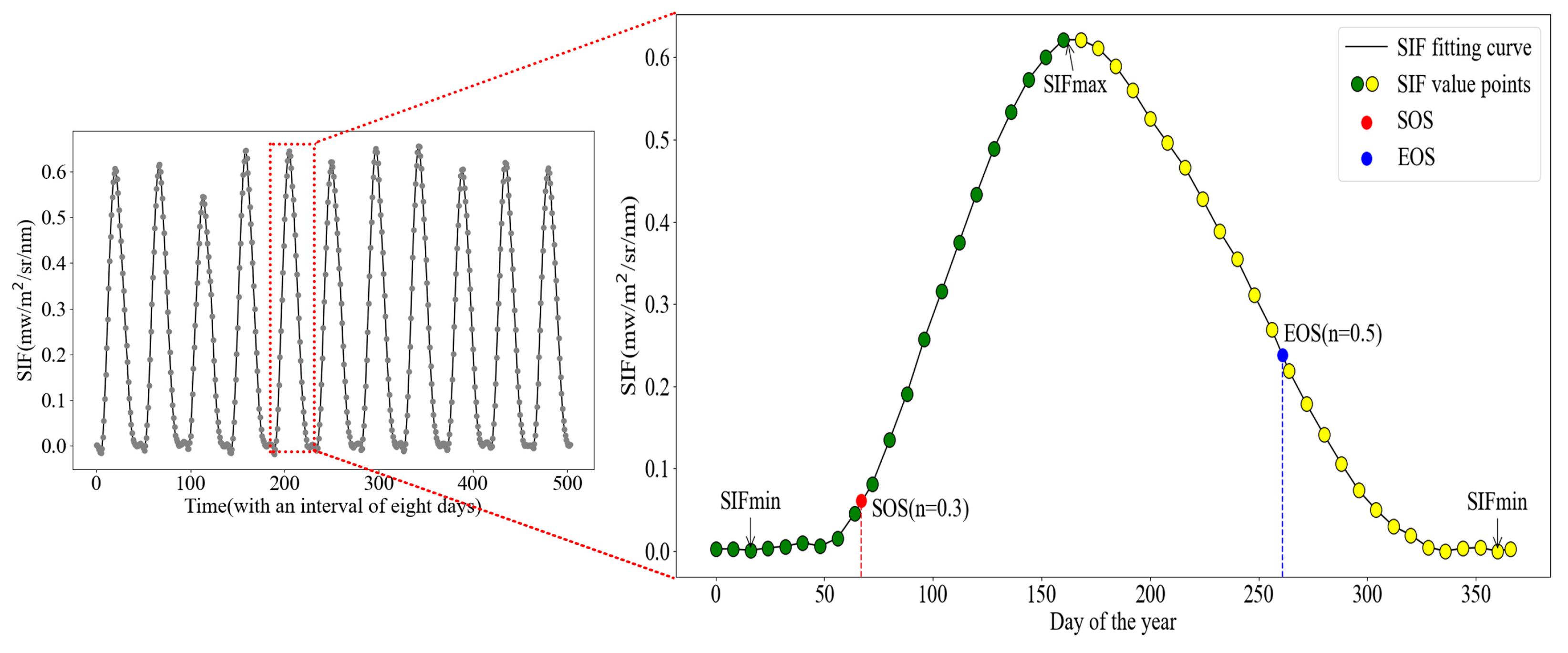
2.3.1. Phenology Extraction

To accurately capture the trend of SIF during the vegetation growth cycle, the SIF data were smoothed using—Savitzky-Golay (S-G) filtering. S-G filtering filters out environmental noise from remotely sensed data, preserving the trend and periodicity characteristics of the data by selecting multiple data points within a neighborhood of the data points and replacing their values using polynomial fitting [53]. Next, we used a cubic smoothing spline model to fit the SIF time series and predict the SIF values for each day of the year [54]. This method can flexibly model the seasonal variation pattern of vegetation while maintaining the smoothness of the curve and effectively reconstructing the seasonal trajectory.

$${\mathrm{S}}_{\mathrm{i}}\left(\mathrm{x}\right)={\mathrm{a}}_{\mathrm{i}}+{\mathrm{b}}_{\mathrm{i}}(\mathrm{x}--{\mathrm{x}}_{\mathrm{i}})+{\mathrm{c}}_{\mathrm{i}}{(\mathrm{x}-{\mathrm{x}}_{\mathrm{i}})}^2+{\mathrm{d}}_{\mathrm{i}}{(\mathrm{x}-{\mathrm{x}}_{\mathrm{i}})}^3$$

(1)

In this equation, x and ${\mathrm{x}}_{\mathrm{i}}$ are the two neighboring points (with a step size of eight days for the SIF data), and ${\mathrm{a}}_{\mathrm{i}}$, ${\mathrm{b}}_{\mathrm{i}}$, ${\mathrm{c}}_{\mathrm{i}}$, and ${\mathrm{d}}_{\mathrm{i}}$ are the fit coefficients of the equation. The value of SIF between each pair of neighboring points is calculated using several cubic polynomials ${\mathrm{S}}_{\mathrm{i}}$.

In this study, vegetation phenology was estimated using the dynamic threshold method, focusing on two primary metrics: the Start of Growing Season (SOS) and the End of Growing Season (EOS). The SOS marks the transition when the plant changes from a dormant or slowed-down state to an active state of growth, while the EOS signifies the shift in plant growth from an active phase to a dormant stage. The determination of SOS and EOS is based on dynamic thresholds, specifically the ratio of the difference between the observed value and the annual minimum to the difference between the annual maximum and the annual minimum [55]. The corresponding dates are recognized as SOS and EOS when this ratio reaches 0.3 and 0.5, respectively [56].

$${\mathrm{f}}_{\mathrm{r}\mathrm{a}\mathrm{t}\mathrm{i}\mathrm{o}}\left(\mathrm{t}\right)={\displaystyle \frac{\mathrm{y}\left(\mathrm{t}\right)-{\mathrm{y}\left(\mathrm{t}\right)}_{\mathrm{m}\mathrm{i}\mathrm{n}}}{{\mathrm{y}\left(\mathrm{t}\right)}_{\mathrm{m}\mathrm{a}\mathrm{x}}-{\mathrm{y}\left(\mathrm{t}\right)}_{\mathrm{m}\mathrm{i}\mathrm{n}}}}$$

(2)

In this equation, t represents the time at which the SIF time series is reconstructed, $\mathrm{y}\left(\mathrm{t}\right)$ denotes the SIF value at time t, and ${\mathrm{y}\left(\mathrm{t}\right)}_{\mathrm{m}\mathrm{i}\mathrm{n}}$ and ${\mathrm{y}\left(\mathrm{t}\right)}_{\mathrm{m}\mathrm{a}\mathrm{x}}$ correspond to the minimum and maximum annual SIF values, respectively.

Figure 3 illustrates a schematic representation of the dynamic threshold method. In this method, the time corresponding to a certain percentage (n) between the lowest point (${\mathrm{S}\mathrm{I}\mathrm{F}}_{\mathrm{m}\mathrm{i}\mathrm{n}}$) and the peak value (${\mathrm{S}\mathrm{I}\mathrm{F}}_{\mathrm{m}\mathrm{a}\mathrm{x}}$) on either side of the SIF fitting curve is labeled as the critical period of the phenology. During the ascending phase of the curve, the time at which the SIF reaches a value corresponding to a set percentage n is defined as the Start of Growing Season (SOS). In contrast, during the descending phase, the point where the SIF value aligns with the same percentage indicates the End of Growing Season (EOS), with the corresponding time marking this transition.

SOS: Start of Growing Season; EOS: End of Growing Season; ${\mathrm{S}\mathrm{I}\mathrm{F}}_{\mathrm{m}\mathrm{a}\mathrm{x}}$: maximum value of Solar-Induced chlorophyll Fluorescence (SIF); ${\mathrm{S}\mathrm{I}\mathrm{F}}_{\mathrm{m}\mathrm{i}\mathrm{n}}$: minimum value of Solar-Induced chlorophyll Fluorescence.

2.3.2. Satellite Phenological Evaluation Based on Ground-Based Observations

We compared phenology data extracted from satellite SIFs with GPP-based phenology data and used mean error (ME), mean absolute error (MAE), and root mean square error (RMSE) as evaluation metrics.

$$\mathrm{M}\mathrm{E}={\displaystyle \frac{1}{\mathrm{n}}}\sum _{\mathrm{i}=1}^{\mathrm{n}}\left({\mathrm{y}}_{\mathrm{i}}-\widehat{{\mathrm{y}}_{\mathrm{i}}}\right)$$

(3)

$$\mathrm{M}\mathrm{A}\mathrm{E}={\displaystyle \frac{1}{\mathrm{n}}}\sum _{\mathrm{i}=1}^{\mathrm{n}}\left|{\mathrm{y}}_{\mathrm{i}}-\widehat{{\mathrm{y}}_{\mathrm{i}}}\right|$$

(4)

$$\mathrm{R}\mathrm{M}\mathrm{S}\mathrm{E}=\sqrt{{\displaystyle \frac{1}{\mathrm{n}}}\sum _{\mathrm{i}=1}^{\mathrm{n}}{\left({\mathrm{y}}_{\mathrm{i}}-\widehat{{\mathrm{y}}_{\mathrm{i}}}\right)}^2}$$

(5)

In Equations (3)–(5), n is the number of years, ${\mathrm{y}}_{\mathrm{i}}$ is the extracted phenological metrics based on different scales of SIF products, $\widehat{{\mathrm{y}}_{\mathrm{i}}}$ is the extracted phenological metrics based on GPP, and i is the given year. The closer these evaluation metrics are to 0, the higher the accuracy of the extracted phenological metrics.

2.3.3. Analysis of Spatial and Temporal Trends in Deciduous Forest Phenology

In this study, the Theil—Sen median (TSM, equivalent to Sen’s slope) method was applied to reveal the dynamics of phenological change in mid- to high-latitude deciduous forests in the Northern Hemisphere. The TSM method is suitable for this type of analysis due to its robustness, making it an effective nonparametric tool for trend assessment of long-term series data with a high tolerance for measurement error and outliers [57,58]. To assess the statistical significance of these trends, we coupled TSM with the Mann-Kendall (MK) test (p < 0.05). The MK test evaluates monotonic trend significance without assuming linearity and is resilient to missing data [59]. The TSM estimation method of SOS/EOS is shown in Equation (6). Here, SOS and EOS denote the start and end of the growing season, respectively. Both are estimated independently using the following equation:

$${\mathrm{S}}_{\mathrm{S}\mathrm{O}\mathrm{S}/\mathrm{E}\mathrm{O}\mathrm{S}}=\mathrm{M}\mathrm{e}\mathrm{d}\mathrm{i}\mathrm{a}\mathrm{n}\left({\displaystyle \frac{{\mathrm{S}\mathrm{O}\mathrm{S}/\mathrm{E}\mathrm{O}\mathrm{S}}_{\mathrm{i}}-{\mathrm{S}\mathrm{O}\mathrm{S}/\mathrm{E}\mathrm{O}\mathrm{S}}_{\mathrm{j}}}{\mathrm{j}-\mathrm{i}}}\right),2008\le \mathrm{i}<\mathrm{j}\le 2017$$

(6)

To verify whether the observed trends in phenology were statistically significant, we further employed the -Mann-Kendall (MK) test in our analysis.

$$\mathrm{Z}=\left\{\begin{array}{c}{\displaystyle \frac{\mathrm{S}-1}{\sqrt{\mathrm{s}\left(\mathrm{S}\right)}}}\\ 0\\ {\displaystyle \frac{\mathrm{S}+1}{\sqrt{\mathrm{s}\left(\mathrm{S}\right)}}}\end{array}\right.,\mathrm{S}>0,\mathrm{S}=\sum _{\mathrm{j}=1}^{\mathrm{n}-1}\sum _{\mathrm{i}=\mathrm{j}+1}^{\mathrm{n}}\mathrm{s}\mathrm{g}\mathrm{n}\left({\mathrm{S}\mathrm{O}\mathrm{S}/\mathrm{E}\mathrm{O}\mathrm{S}}_{\mathrm{j}}-{\mathrm{S}\mathrm{O}\mathrm{S}/\mathrm{E}\mathrm{O}\mathrm{S}}_{\mathrm{i}}\right)$$

(7)

$$\mathrm{S}\mathrm{g}\mathrm{n}\left({{\displaystyle \frac{\mathrm{S}\mathrm{O}\mathrm{S}}{\mathrm{E}\mathrm{O}\mathrm{S}}}}_{\mathrm{j}}-{{\displaystyle \frac{\mathrm{S}\mathrm{O}\mathrm{S}}{\mathrm{E}\mathrm{O}\mathrm{S}}}}_{\mathrm{i}}\right)=\left\{\begin{array}{c}1,{{\displaystyle \frac{\mathrm{S}\mathrm{O}\mathrm{S}}{\mathrm{E}\mathrm{O}\mathrm{S}}}}_{\mathrm{j}}-{{\displaystyle \frac{\mathrm{S}\mathrm{O}\mathrm{S}}{\mathrm{E}\mathrm{O}\mathrm{S}}}}_{\mathrm{i}}>0\\ 0,{{\displaystyle \frac{\mathrm{S}\mathrm{O}\mathrm{S}}{\mathrm{E}\mathrm{O}\mathrm{S}}}}_{\mathrm{j}}-{{\displaystyle \frac{\mathrm{S}\mathrm{O}\mathrm{S}}{\mathrm{E}\mathrm{O}\mathrm{S}}}}_{\mathrm{i}}=0\\ -1,{{\displaystyle \frac{\mathrm{S}\mathrm{O}\mathrm{S}}{\mathrm{E}\mathrm{O}\mathrm{S}}}}_{\mathrm{j}}-{{\displaystyle \frac{\mathrm{S}\mathrm{O}\mathrm{S}}{\mathrm{E}\mathrm{O}\mathrm{S}}}}_{\mathrm{i}}<0\end{array}\right.,\mathrm{s}\left(\mathrm{S}\right)={\displaystyle \frac{\mathrm{n}\left(\mathrm{n}-1\right)\left(2\mathrm{n}+5\right)}{18}}$$

(8)

In Equations (7) and (8), ${\mathrm{S}\mathrm{O}\mathrm{S}/\mathrm{E}\mathrm{O}\mathrm{S}}_{\mathrm{i}}$ and ${\mathrm{S}\mathrm{O}\mathrm{S}/\mathrm{E}\mathrm{O}\mathrm{S}}_{\mathrm{j}}$ denote $\mathrm{S}\mathrm{O}\mathrm{S}/\mathrm{E}\mathrm{O}\mathrm{S}$ for year i and year j, respectively; the function $\mathrm{“}\mathrm{s}\mathrm{g}\mathrm{n}\mathrm{”}$ refers to the sign function; while $\mathrm{n}$ refers to the span of the time series. The statistic $\mathrm{Z}$ can take values from $(-\mathrm{\infty },+\mathrm{\infty })$. For a specified significance level $\mathsf{\alpha }$, a trend change is considered statistically significant when $\left|\mathrm{Z}\right|>{\mathrm{u}}_{1-{\displaystyle \frac{\mathsf{\alpha }}{2}}}$. The statistical significance of the trend variation in the $\mathrm{S}\mathrm{O}\mathrm{S}/\mathrm{E}\mathrm{O}\mathrm{S}$ time series was evaluated using a confidence level $\mathsf{\alpha }$ = 0.05. This study investigates the trends in phenological metrics derived from various SIF products for deciduous forests in the mid- and high-latitudes of the Northern Hemisphere, covering the period from 2008 to 2017. Additionally, we conducted a comparison and assessment of the variations in the trends between the two phenological metrics.

2.3.4. Response of Deciduous Forest Phenology to Climatic Factors

Because vegetation phenology is strongly influenced by the preseasonal climate, it is commonly used to examine how phenology responds to various climate variables [60,61]. The preseason length is determined by calculating Spearman’s correlation coefficient and is defined as the period from the most sensitive period of vegetation phenology to the month in which the phenological metric occurs. This period occurs 1 to 4 months prior to the multi-year average of the start or end of the growing season (SOS/EOS) [62,63,64]. Preseason duration for 2m temperature is defined as the period (in steps of 1 month) before the multi-year average of SOS/EOS during which the maximum bias correlation coefficient occurs between SOS/EOS and 2m temperature after excluding the influence of climatic factors such as precipitation and soil temperature during the same period. We performed similar steps for other climatic factors.

In this study, we used SHapley Additive exPlanations (SHAP) analysis to explore the response of the 1-km and 5-km SIF products’ extracted phenological SOS/EOS metrics to individual climatic factors. SHAP analysis is a machine-learning interpretation tool based on the principles of cooperative game theory [65], which can reveal the complex relationships in deciduous forests between phenology and climatic factors. By assessing the relative importance of each climatic factor in phenological change and evaluating the influence of each climatic factor on the phenological prediction model, the method provides insights into how climatic factors drive phenological changes in deciduous forests, offering a comprehensive and detailed explanatory framework for analysis and comparison at different scales.

3. Results

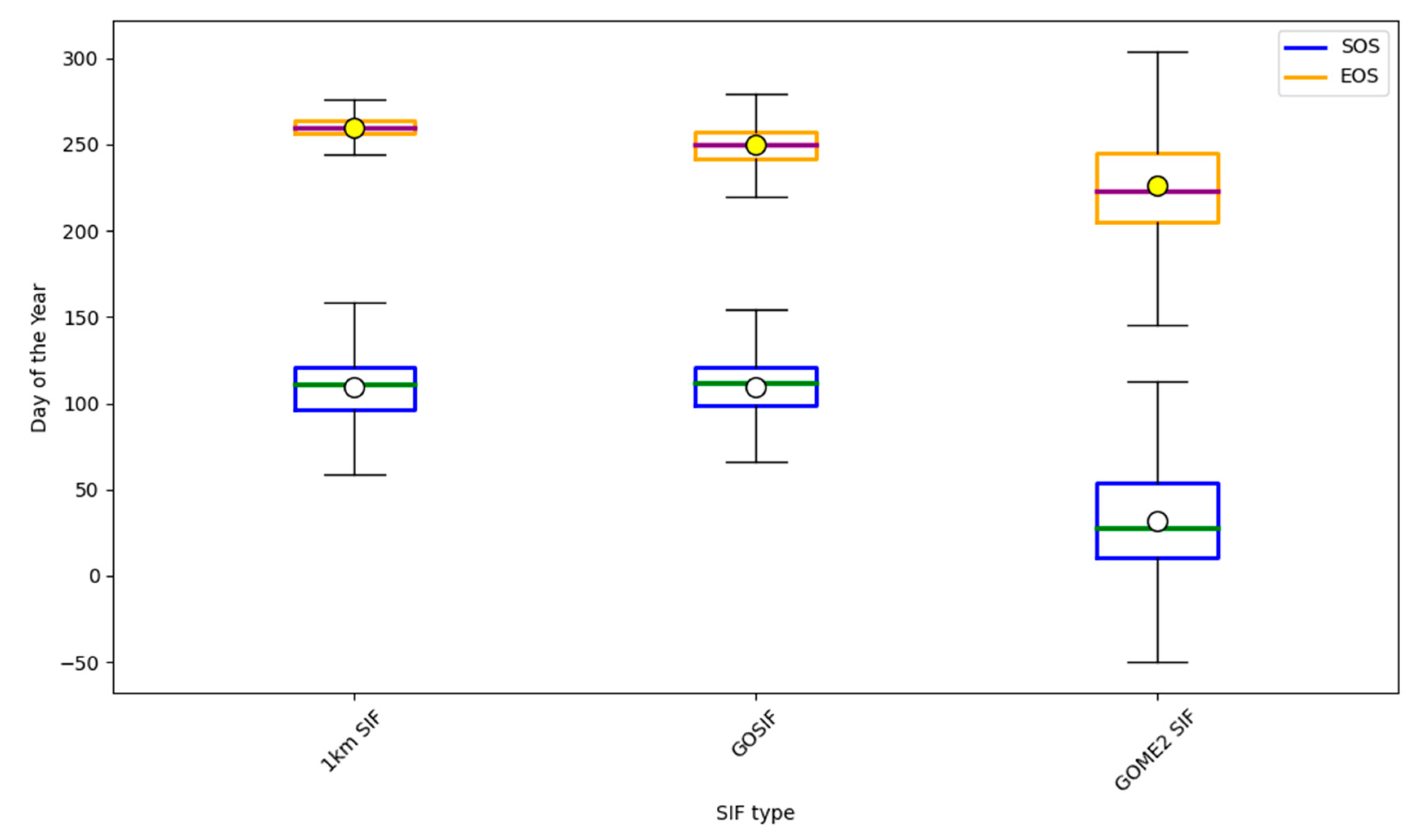
3.1. Analysis and Comparison of Phenology Extracted from SIF Data at Different Scales

Using data from 16 flux stations, we present the statistical results of phenological metrics extraction from three different resolutions of SIF data in Table S2 of the Supporting Information. The phenological results extracted from the GRSIF001 data show that the mean error (ME) at the Start of Growing Season (SOS) is −0.16 days, with a mean absolute error (MAE) of 4.48 days and a root mean square error (RMSE) of 5.39 days. The ME at the End of Growing Season (EOS) is −15.49 days, with an MAE of 15.49 days and an RMSE of 16.99 days. These results are based on 45 phenological data points from 9 research sites. The ME of SOS extracted from GOSIF data is 6.76 days, with an MAE of 9.20 days and an RMSE of 12.60 days. The ME of EOS is −21.07 days, with an MAE of 21.07 days and an RMSE of 22.10 days. These results are based on 42 phenological data points from 7 research sites. The ME of SOS extracted from GOME-2 SIF data is −58.48 days, with an MAE of 58.94 days and an RMSE of 63.00 days. The ME of EOS is −42.73 days, with an MAE of 42.73 days and an RMSE of 45.99 days. These results are based on 48 phenological data points from 8 research sites. These results demonstrate the level of consistency with the phenological data extracted from GPP sites, indicating the capacity of SIF data to track phenological metrics.

Three different resolutions of SIF data were comprehensively statistically analyzed between 2008 and 2017, and Figure 4 demonstrates the distribution of day-year (DOY) for the phenological metrics SOS and EOS, computed by the SIF products over a year. Overall, the consistency between the phenological metrics calculated based on GRSIF001 and GOSIF is high, with the earliest SOS occurring around day 50 and the latest at approximately day 150, and the earliest EOS occurring around day 210 and the latest at approximately day 280. In contrast, the alignment of phenological metrics derived from GOME-2 SIF with those obtained from the other two sources was weaker, with SOS ranging from as early as day 315 of the prior year to as late as day 100 of the subsequent year, and EOS as early as about day 150 and as late as about day 300. This discrepancy is primarily attributed to the lower spatial resolution of GOME-2 SIF, which limits its ability to capture localized phenological variations and results in reduced consistency compared to the higher-resolution SIF products.

3.2. Temporal and Spatial Distribution of Phenology

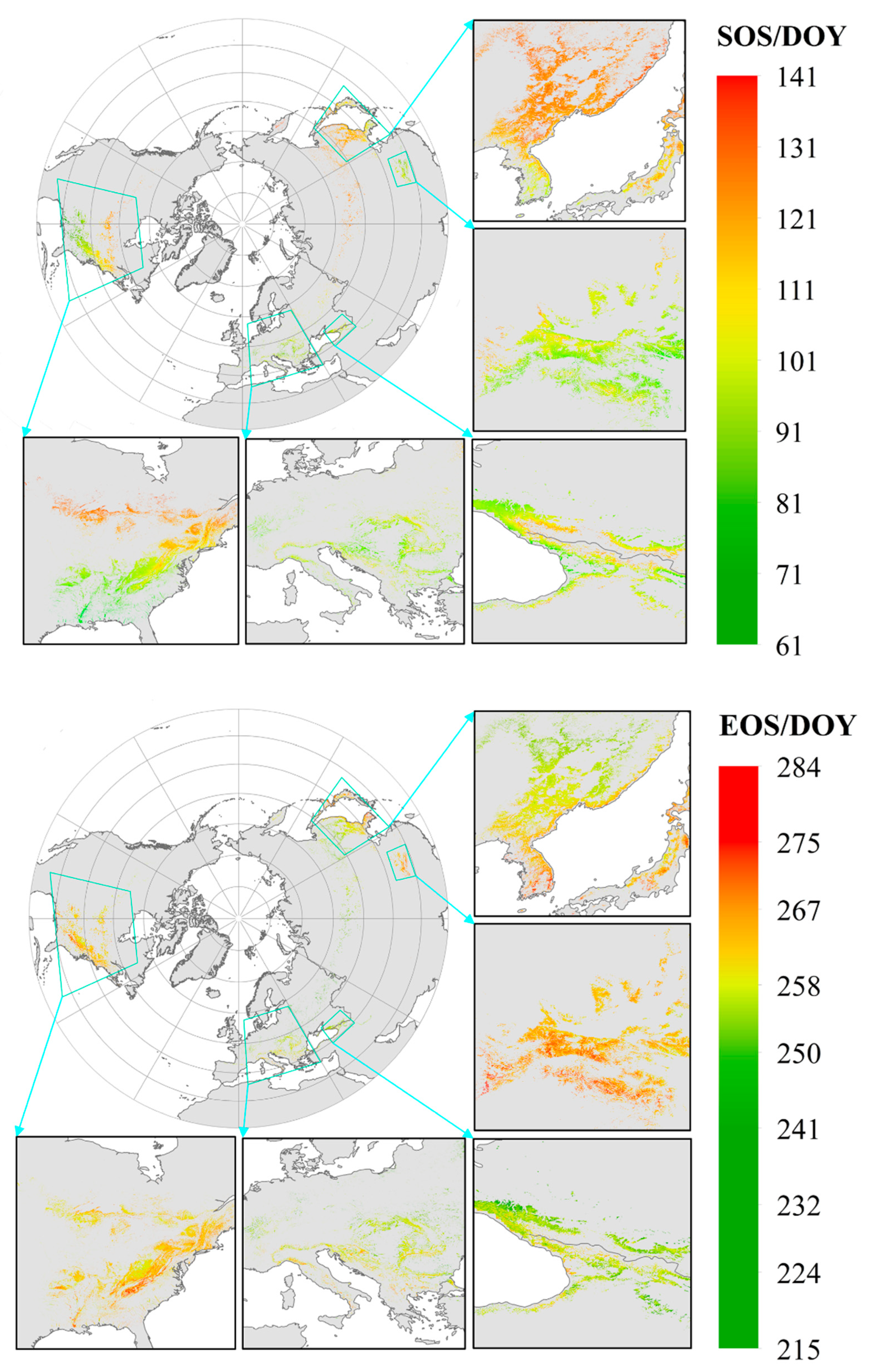
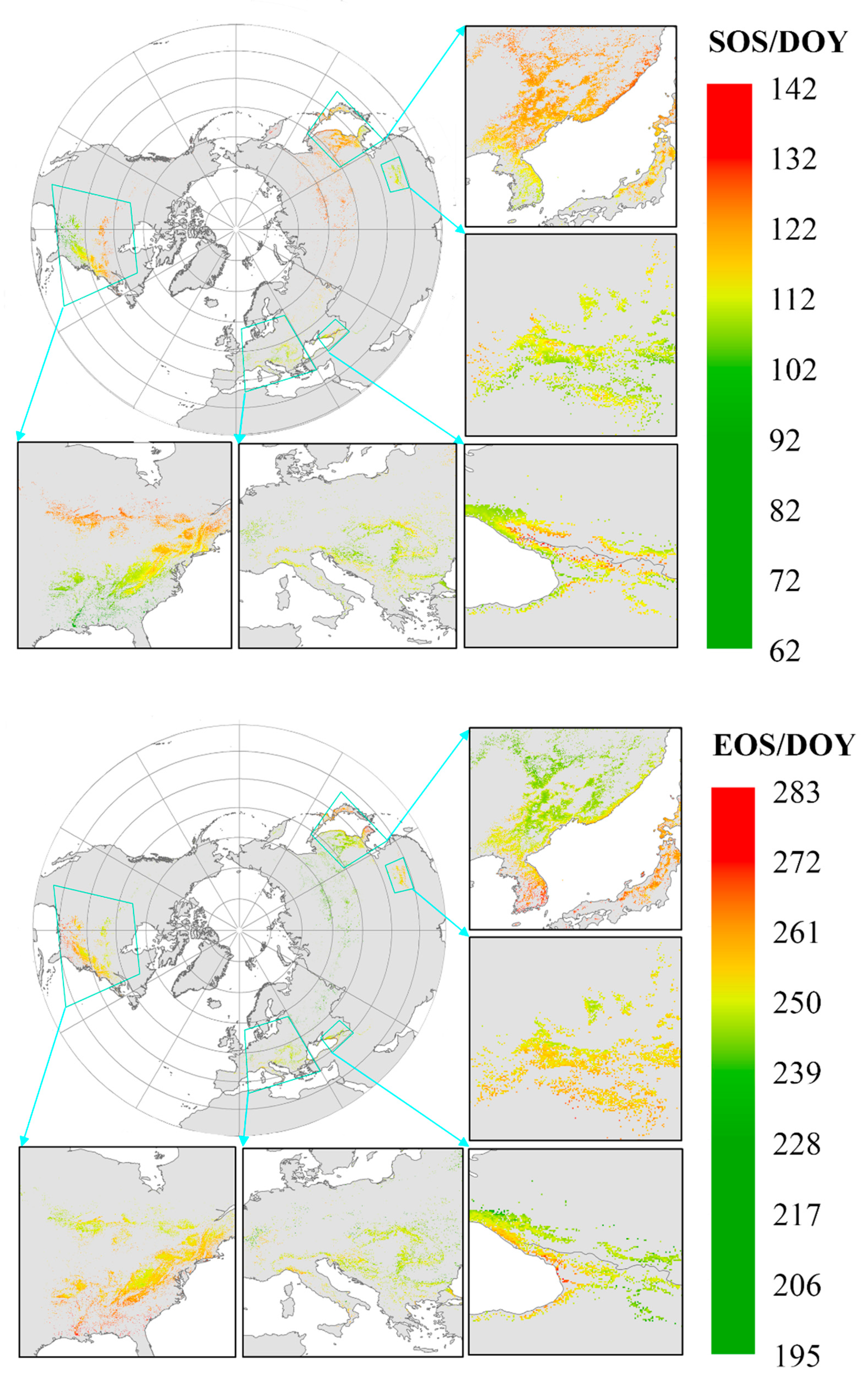
3.2.1. Spatial Distribution of Phenology

Using the phenological information extracted from SIF data at different resolutions, this study determined the pixel mean values of the phenological metrics SOS and EOS for deciduous forests across the Northern Hemisphere’s middle and high latitudes during 2008–2017. The spatial distribution of these mean values over the ten-year period is shown in Figure 5, Figure 6 and Figure 7. It was found that the SOS and EOS of deciduous forests in the middle and high latitudes of the Northern Hemisphere indicate significant spatial heterogeneity.

From Figure 5, Figure 6 and Figure 7, it can be seen that, in general, the phenological changes of deciduous forests are closely related to latitude. With increasing latitude, the SOS of deciduous forests was gradually delayed while the EOS was gradually advanced, a phenomenon consistent with the findings of [66], and this latitudinal dependence may be related to the latitudinal gradient of climatic factors, such as sunshine hours, temperature, and precipitation. In the study area, the multi-year mean SOS of the deciduous forest extracted from the 1-km resolution SIF data ranged from day 61 to day 141, while the multi-year mean EOS ranged from day 215 to day 284. Over the years, the regions with the earliest SOS were centered in the southeastern U.S. (ca. day 70), Eastern Europe (ca. day 90), and the Black Sea coast (ca. day 95), while the regions with the latest SOS were located in the northern U.S. (ca. day 120) and East Asia (ca. day 125). The regions with the earliest EOS were centered in the northeastern central part of the U.S. (ca. day 240), Eastern Europe (ca. day 245), and Central Asia (ca. day 250), while the latest emergence regions are in the southeastern United States (ca. day 270), southern China (ca. day 275), the Korean Peninsula (ca. day 285), and the Japanese islands (ca. day 270). The observed spatial distribution pattern could be influenced by the climatic conditions and soil types prevalent in these regions. For example, the humid subtropical climate in the southeastern United States, where soils are mostly black or red and cool slowly, combined with abundant rainfall and long frost-free periods [67], results in the local deciduous forests having an early onset of the growing season and a late end of the growing season. In the 5-km resolution GOSIF data, the extracted multi-year average SOS of deciduous forests extends from day 62 to day 142, while the multi-year average EOS extends from day 195 to day 283. The spatial distribution pattern of phenology does not differ significantly from that of the phenology features extracted from the 1-km resolution SIF data. However, the range of SOS/EOS values extracted from the 50-km resolution GOME-2 SIF differed significantly from the two previously mentioned datasets. Specifically, its annual mean SOS is distributed from day −6 to day 92, while the multi-year mean EOS is located between day 190 and day 254. This suggests that the vegetation growth cycle revealed by the GOME-2 SIF is more advanced relative to the high-resolution SIF data, such that the SOS sometimes occurs at the end of the previous year.

In summary, there are differences in the ability to reveal phenological characteristics of deciduous forests between datasets of different resolutions. The higher-resolution data (1 km and 5 km) provided more precise phenological information, while the lower-resolution data (50 km) may have underestimated the timing of phenological events because of the mixed pixel effect. Although data at different resolutions captured general trends in phenological changes, the 1-km resolution data had a clear advantage in providing detailed and regionally specific information.

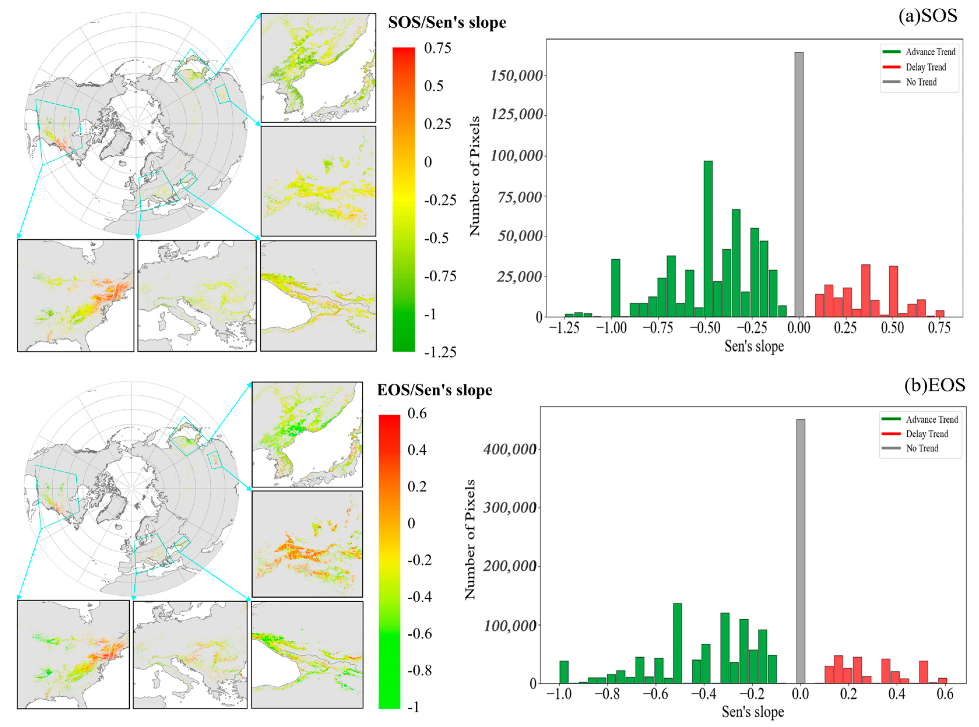
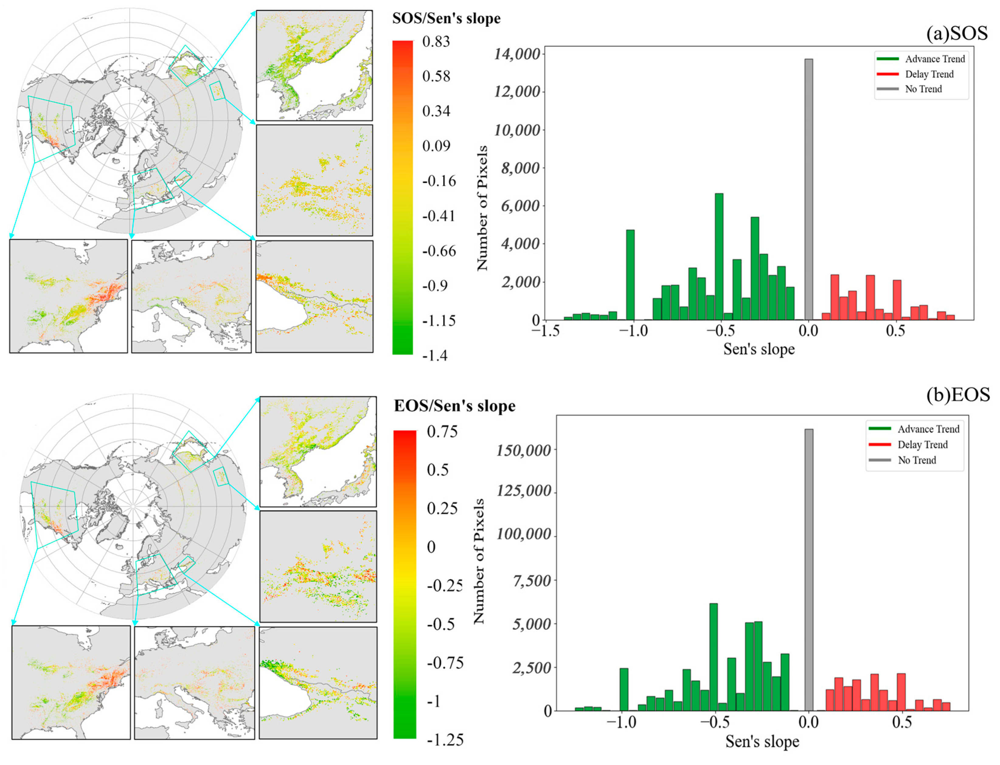
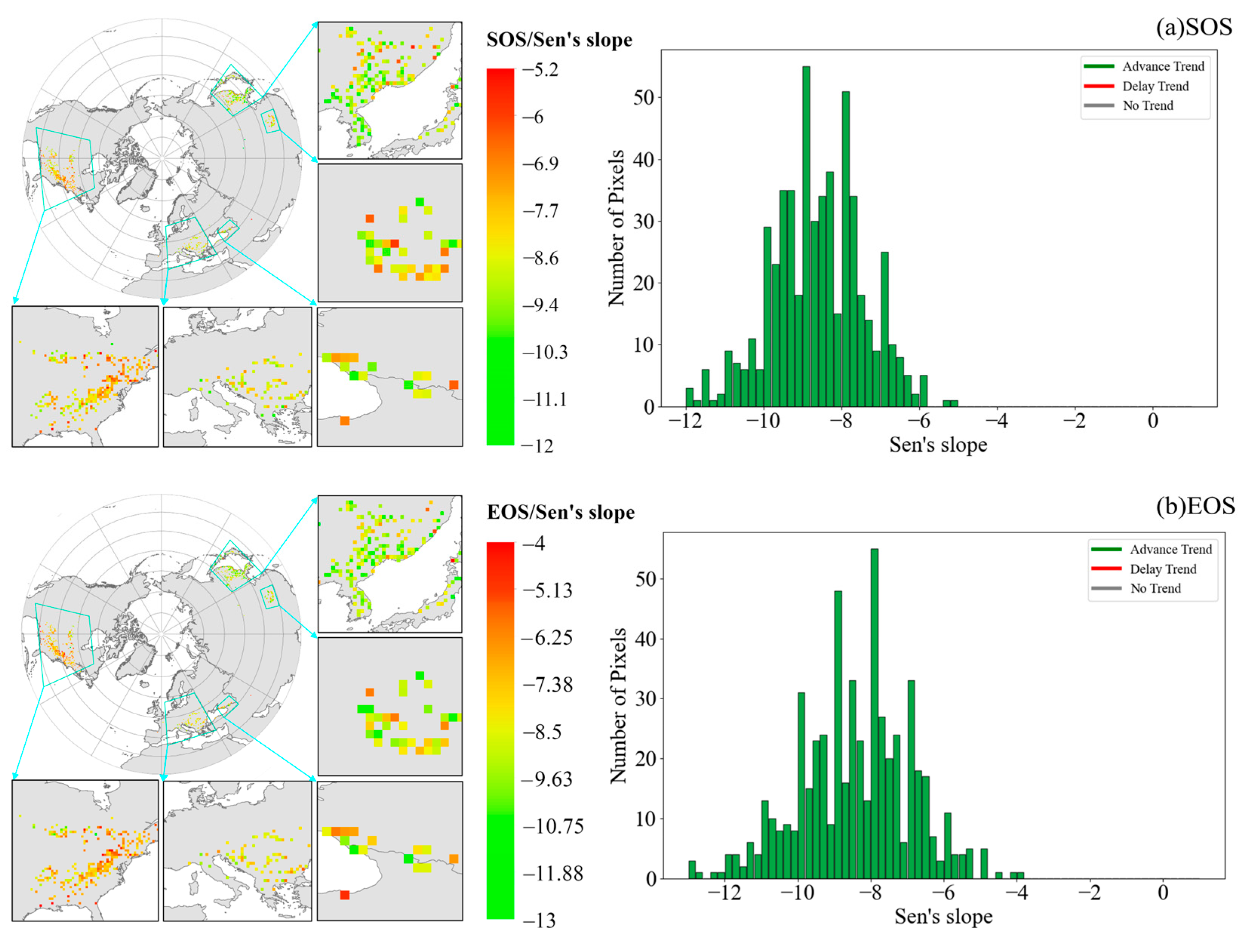
3.2.2. Trends in Temporal and Spatial Patterns of Phenology

To quantify the trend of vegetation phenology, the Sen’s slope factor was utilized in this study. The spatial distribution pattern of the Sen’s slope factor of the phenological metrics extracted from the 1-km SIF across the study region is provided in Figure 8. It was found that the SOS of mid- to high-latitude deciduous forests in the Northern Hemisphere from 2008 to 2017 had an overall advance trend, with an average Sen’s slope factor of −0.229, in which the range of advancement (62.62%) and significant advancement (2.42%) was greater than the range of delay (18.94%) and significant delay (0.17%), respectively. EOS also has an overall advance trend, with an average Sen’s slope factor of −0.181, where the range of advancement (55.87%) and significant advancement (4.91%) is greater than the range of delay (16.81%) and significant delay (0.15%), respectively. Although the proportion of significantly advanced areas is relatively small, their wide distribution reflects the response of deciduous forest ecosystems to environmental changes in the context of global warming.

Spatially, SOS advancement is predominantly observed in the eastern and northern parts of the U.S., southern Europe, the Black Sea coast, Central Asia, and East Asia. The regions with SOS postponement are mainly located in the northeastern and southern U.S., the northeastern Middle East, and Eastern Europe. The regions with EOS advancement are mainly situated in the northern and southeastern regions of the U.S., the northeastern Middle East, and northeastern China. The areas exhibiting EOS postponement were mainly in the northeastern U.S., Eastern Europe, and Central China. The trend of advancement of phenological metrics in most of the regions may be related to global warming, where a rise in overall temperature could cause plants to start growing earlier, thus entering the beginning of the growing season earlier (SOS), and similarly, this increase in temperature may cause plants to complete the growth cycle earlier, thus ending the growing season earlier (EOS) [68]. Regions showing delays in phenological metrics may be doing so because of complex interactions of localized climatic conditions, soil moisture, or land use changes, such as the combination of changing temperature and precipitation patterns and extreme weather events in the northeastern United States resulting in a delayed phenological period in local deciduous forests [69]. These local variations highlight the spatial heterogeneity of phenological changes and add to the complexity of accurate ecological predictions and the development of adaptive management strategies.

In this study, in addition to the 1-km SIF dataset, the GOSIF and GOME-2 SIF datasets were used for the TSM-MK method (Figure 9 and Figure 10). The results show that using the coarser spatial resolution of the SIF data resulted in a more pronounced trend in the advancement of phenology. Among them, the SOS extracted from GOSIF showed an overall advance trend with an average Sen’s slope of −0.264, where the proportion of advance (62.42%) and significant advance (2.36%) was greater than the range of delay (18.71%) and significant delay (0.10%), respectively. EOS, on the other hand, likewise has an overall advance trend with an average Sen’s slope of −0.187, where the range of advancement (56.73%) and significant advancement (2.93%) is greater than the range of delay (20.75%) and significant delay (0.20%), respectively. In addition, the GOME-2 SIF extracted SOS and EOS showed an advance trend for all pixels, with an average Sen’s slope of −8.644 and −8.448 for SOS and EOS, respectively. Figure 11 shows a comparison of phenological trends extracted from three different scales of SIF.

3.3. Results of Phenological Responses to Climate

We used SHAP analysis to reveal the effects of each climatic factor on the phenology (SOS/EOS) of deciduous forests in mid- and high-latitude regions of the Northern Hemisphere extracted from 1-km and 5-km SIF data, and the results are shown in Figure 12 and Figure 13. We plotted beeswarm plots of SHAP values and histograms of feature importance to show the contribution of each climatic factor to the model predictions and its average feature importance, respectively. The beeswarm plots display the distribution of SHAP values for each climatic factor, with colors indicating the magnitude of the values, distinguishing between facilitating and inhibiting effects. The histograms show the average SHAP values for each climatic factor, which serve as the basis for the importance ranking.

Overall, temperature (both air and soil temperature) is the key factor driving the variation in SOS in mid- to high-latitude deciduous forests in the Northern Hemisphere, followed by radiation and precipitation. For EOS, temperature, moisture (soil water content and precipitation), and radiation are the key meteorological factors.

Among the climatic factors affecting the SOS extracted from the 1-km SIF, soil temperature in layer 4 (TS4) was the most critical factor, closely followed by climatic factors such as T2M, soil temperature in layer 3 (TS3), D2M, and PAR. Among these climatic factors, TS4, T2M, TS3, and D2M had a significant negative effect on SOS, suggesting they contribute to its advancement. In contrast, variables such as PAR, PRE, and soil water content in layer 1 (SWC1) inhibited the advancement of SOS. For EOS, TS4 was again the primary influencing factor, followed by climatic factors, including D2M, the soil water content in layer 4 (SWC4), VPD, PRE, and PAR. Among these factors, TS4, D2M, SWC4, PRE, and PAR tended to delay EOS, while VPD promoted the advancement of EOS. Compared with the 1-km results, the evaluation of the phenological metrics (SOS/EOS) derived from the 5-km SIF, as influenced by climatic factors, showed that the response mechanism of each climatic factor to the phenological metrics remained unchanged. However, there was a change in the order of importance: among the SOS indicators, soil temperature in layer 3 (TS3) was more important than T2M, while among the EOS indicators, soil water content in layer 4 (SWC4) was more important than D2M.

4. Discussion

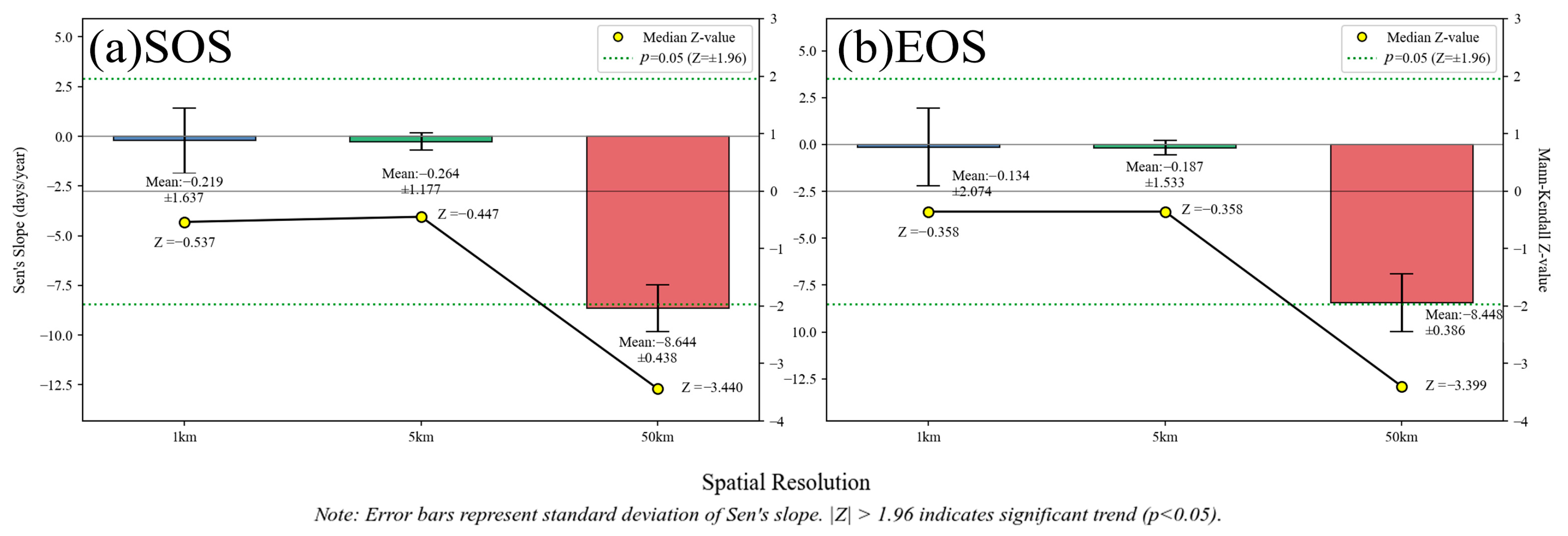
4.1. Comparison and Analysis of Phenological Characteristics at Different Scales

The phenological metrics extracted from SIF data with three different spatial resolutions revealed the significant influence of spatial scale in the phenological tracking process of deciduous forests. Specifically, the use of 1-km resolution SIF products in tracking phenological metrics of deciduous forests, such as the SOS and EOS, showed significant improvement. These products demonstrated better consistency with results extracted from the GPP sites compared to the 5-km and 50-km resolution SIF products (Table S2). This can be attributed to the fact that phenological data obtained from satellite imagery incorporate details from all features within a pixel. As high-resolution data, the 1-km SIF captures detailed vegetation information because its smaller pixel coverage allows more precise detection of localized changes and better differentiation of growth stages. In contrast, coarse-resolution surface phenology inversions consistently exhibit the mixing effects of different vegetation components [36,70,71]. Compared to the 1 km window, the content of deciduous forest pixels within the 5 km and 50 km windows decreased by 27.48% and 36.99%, respectively. The coarse-resolution SIF data may not be able to effectively distinguish vegetation heterogeneity, resulting in more ambiguous phenology information extracted (Figure 7). Prior studies have indicated that when vegetation in a proportion of high-resolution pixels begins greening, the detected coarse-resolution SOS corresponds to the earlier stages of high-resolution SOS pixels [37]. This may explain why coarse-resolution SIF tends to underestimate phenological metrics. The source area footprint of the flux tower is less than a 1000-m radius, which better matches the 1 km spatial scale and shows significant scale differences with 5 km/50 km. This is another key driver of the scale effect: coarse-resolution pixels, containing a large amount of heterogeneous land surface (e.g., cropland, bare soil) outside the flux tower source area, intrinsically exhibit a weakened correlation between their SIF signal and tower-based GPP. In addition, the differences in phenological metrics between SIF data at different spatial resolutions may be influenced by the degree of landscape fragmentation [30]. Landscape fragmentation may lead to the disruption of the continuity of deciduous forest ecosystems, thus affecting the measurement of phenological metrics. Future research should focus on improving algorithms for generating such high-resolution SIF products and conducting comprehensive assessments of their effectiveness for application to a wider range of vegetation types and environmental conditions [72].

When comparing and analyzing the phenological data across scales, we recognize that scale selection is critical to capture trends in phenological changes. At a 1-km resolution, SIF data can accurately capture complex geographic details and local ecological shifts, facilitating the identification of subtle variations in phenological metrics (Figure 8). However, at coarser resolutions, such as those of the GOSIF and GOME-2 SIF datasets, the trend of phenological advancement becomes more evident (Figure 9 and Figure 10). This is because coarser-scale data integrate more spatial information and reduce local noise and variability [73]. As a result, coarse-scale data may ignore local fluctuations, thus providing a clearer perspective on ecological patterns and trends at large scales. The comparative analysis underscores the significant role of scale effects in phenology research: the fine scale facilitates in-depth exploration of local ecological processes, while the coarse scale is more suitable for identifying trends in macroscopic ecological change. Therefore, researchers must carefully consider the spatial scale of their research questions and select the appropriate data resolution to ensure that the trends of phenological change can be accurately captured and interpreted.

4.2. Response of Phenology to Climatic Factors

We compared how phenological metrics respond to climatic factors at 1-km and 5-km spatial resolution to assess the impact of scale on phenological responses to climate. The results indicate that scale effects did not significantly influence the analysis. Although the finer scale of 1 km allowed us to obtain more detailed geographic information, the coarser scale of 5 km may have smoothed local features [74], resulting in different representations of climatic factors at the two scales, and the response mechanism between climatic factors and phenological metrics remained consistent across both scales, suggesting that climate change has a generalized effect on phenology. As shown in Figure 12 and Figure 13, it is noteworthy that at the 1-km scale, the importance of T2M in SOS exceeds that of TS3, and the importance of D2M in EOS exceeds that of SWC4, which demonstrates that the importance of climatic factors varies at different scales. In addition, the consistency of the direction of influence is also confirmed, e.g., the negative influence of TS4, T2M, etc., on SOS and the positive influence of VPD on EOS remain consistent across both scales. Supporting our findings, Liu and Zhang (2020) showed that, despite potential spatial smoothing at coarser resolutions, the underlying climatic drivers of phenological changes produced consistent responses across regions [75]. Therefore, we conclude that the phenological metrics extracted from SIF data at different spatial resolutions responded to them to a similar extent when using preseason climatic factors calculated with monthly time steps, and the observed differences fall within acceptable limits. This study enhances our comprehension of how climatic factors influence phenological metrics at varying scales and establishes a scientific foundation for ecological monitoring and the development of climate change adaptation strategies.

Environmental factors interact and jointly influence the developmental rhythm of deciduous forests. Earlier studies have indicated that phenological metrics (e.g., SOS and EOS) are primarily regulated by temperature [76,77,78,79]. Furthermore, precipitation and solar radiation are key factors affecting EOS in some ecosystems [80]. In the case of our study, air and soil temperatures influenced the phenology metrics more than other environmental factors, and the dominant effect of soil temperature on phenology aligns with the previous findings of [44]. The temporal and spatial trends of each climatic variable for the period of 2008–2017 are plotted in Figure S2 in the Supporting Information. Among the many factors affecting phenology, soil and air temperature are the most critical. The rise in soil and air temperatures in spring accelerates heat accumulation, especially in the soil layer where deciduous forest roots are located, to satisfy the need for temperature accumulation and promote the advancement of phenology [81]. High-temperature soil enhances root uptake, accelerates growth, and delays fall phenology [81]. Differences in soil moisture affect soil temperature changes, and reducing moisture accelerates soil temperature rise [82], promoting the early spring development of deciduous forests. Dry soils increase root heat uptake and accelerate plant awakening and growth, but reduced moisture reserves may limit plant growth [83]. Low humidity may also advance fall phenology, as plants accelerate dormancy and defoliation in response to drought [84]. Increased winter precipitation alters the heat balance at the surface and the process of heat accumulation in the spring, leading to a delay in spring phenology [85]. Increased precipitation during the late summer may lead to slower surface heat dissipation, thus delaying fall phenology in deciduous forests [86]. In spring, when VPD is low and air humidity is high, elevated VPD enhances transpiration and promotes growth. However, when the VPD level is too high, plants tend to close their stomata, which in turn slows down their growth [87]. High VPD in the fall accelerates water loss, prompting plants to enter dormancy and leaf drop rapidly [87]. Increased radiation in spring accelerates soil heating, the activity of root systems, and earlier shoot growth, leading to earlier SOS [88]. A lower solar altitude angle in the fall shortens sunlight and reduces radiation [89], limiting photosynthesis and contributing to earlier EOS [90]. An in-depth understanding of the changes in soil temperature and other elements, and their effects on plant growth, is of vital significance for the scientific management of forestry resources and the maintenance of ecological balance.

4.3. Limitations, Uncertainties, and Prospects

This study primarily aims to reveal the differences among the conclusions drawn using SIF datasets with different spatial resolutions. However, the relatively low spatial resolution of the climate data we used may limit the ability to capture higher spatial heterogeneity, potentially restricting remote sensing’s capacity to explore the mechanisms behind vegetation dynamics at various scales. In addition, the varying resolutions of SIF data used in this research may lead to variations in data quality and extracted phenological metrics due to differences in satellite platforms, sensors, and data-processing methods [91], introducing potential uncertainties.

Climate change is not only influenced by conventional climatic factors but may also be affected by extreme climatic events such as high temperatures, floods, droughts, and other uncertainties [34,66,83,92,93,94,95,96]. These extreme climatic events may have a significant impact on phenology. In future studies, the use of SIF products at different scales should be considered to analyze the different degrees of response of phenology to climatic and environmental factors, especially under different stressful environmental conditions.

This will help us better understand the complexity of phenological changes and facilitate the effective use of SIF data across various applications, thereby better supporting ecosystem management and environmental protection efforts to ensure ecosystem health and sustainability.

5. Conclusions

In this study, we extracted phenological information from three different spatial resolution SIF products for deciduous forests across the Northern Hemisphere’s middle and high latitudes and analyzed the spatial distribution of the phenological metrics SOS and EOS and their spatio-temporal trends. Meanwhile, this study revealed the potential mechanism of the SIF products by exploring their responses to climate conditions at different spatial resolutions. The results showed that the 1-km resolution SIF products were significantly better than the 5-km and 50-km resolution products in tracking the phenological patterns of deciduous forests, and this advantage was closely related to the spatial scale. In addition, the phenological metrics (SOS/EOS) of deciduous forests in the mid- and high-latitude regions of the Northern Hemisphere generally showed an advance trend from 2008 to 2017, which was demonstrated by SIF products with different resolutions, and the coarser spatial resolution of SIF data made the advance trend of climatic change more obvious. Among the climatic factors affecting phenology, soil temperature in layer 4 was the primary factor, and the response patterns of phenological metrics to climatic factors were similar when derived at different scales. These findings provide an important reference for a deeper understanding of surface phenology. When tracking phenology, we suggest that the effects of SIF products at different scales on the extraction of phenology metrics should be carefully considered in order to optimize the capacity of satellite SIF data to monitor phenology in different application scenarios.

References

1. Ma, H.; Crowther, T.W.; Mo, L.; Maynard, D.S.; Renner, S.S.; Van den Hoogen, J.; Zou, Y.; Liang, J.; De-Miguel, S.; Nabuurs, G. The global biogeography of tree leaf form and habit. Nat. Plants 2023, 9, 1795–1809. [Google Scholar] [CrossRef] [PubMed]
2. Pan, Y.; Birdsey, R.A.; Fang, J.; Houghton, R.; Kauppi, P.E.; Kurz, W.A.; Phillips, O.L.; Shvidenko, A.; Lewis, S.L.; Canadell, J.G. A large and persistent carbon sink in the world’s forests. Science 2011, 333, 988–993. [Google Scholar] [CrossRef]
3. Houghton, R.A. Balancing the global carbon budget. Annu. Rev. Earth Planet. Sci. 2007, 35, 313–347. [Google Scholar] [CrossRef]
4. Luyssaert, S.; Inglima, I.; Jung, M.; Richardson, A.D.; Reichstein, M.; Papale, D.; Piao, S.L.; Schulze, E.D.; Wingate, L.; Matteucci, G. CO2 balance of boreal, temperate, and tropical forests derived from a global database. Glob. Change Biol. 2007, 13, 2509–2537. [Google Scholar] [CrossRef]
5. Baldocchi, D.D.; Wilson, K.B. Modeling CO2 and water vapor exchange of a temperate broadleaved forest across hourly to decadal time scales. Ecol. Model. 2001, 142, 155–184. [Google Scholar] [CrossRef]
6. Chuine, I. A unified model for budburst of trees. J. Theor. Biol. 2000, 207, 337–347. [Google Scholar] [CrossRef]
7. Myneni, R.B.; Keeling, C.D.; Tucker, C.J.; Asrar, G.; Nemani, R.R. Increased plant growth in the northern high latitudes from 1981 to 1991. Nature 1997, 386, 698–702. [Google Scholar] [CrossRef]
8. Yongshuo, F.U.; Jing, Z.; Zhaofei, W.U.; Shouzhi, C. Vegetation phenology response to climate change in China. J. Beijing Norm. Univ. (Nat. Sci.) 2022, 58, 424–433. [Google Scholar]
9. Tucker, C.J. Red and photographic infrared linear combinations for monitoring vegetation. Remote Sens. Environ. 1979, 8, 127–150. [Google Scholar] [CrossRef]
10. Wang, X.; Piao, S.; Xu, X.; Ciais, P.; MacBean, N.; Myneni, R.B.; Li, L. Has the advancing onset of spring vegetation green-up slowed down or changed abruptly over the last three decades? Glob. Ecol. Biogeogr. 2015, 24, 621–631. [Google Scholar] [CrossRef]
11. Wu, C.; Hou, X.; Peng, D.; Gonsamo, A.; Xu, S. Land surface phenology of China’s temperate ecosystems over 1999–2013: Spatial-temporal patterns, interaction effects, covariation with climate and implications for productivity. Agric. For. Meteorol. 2016, 216, 177–187. [Google Scholar] [CrossRef]
12. Wu, C.; Peng, D.; Soudani, K.; Siebicke, L.; Gough, C.M.; Arain, M.A.; Bohrer, G.; Lafleur, P.M.; Peichl, M.; Gonsamo, A. Land surface phenology derived from normalized difference vegetation index (NDVI) at global FLUXNET sites. Agric. For. Meteorol. 2017, 233, 171–182. [Google Scholar] [CrossRef]
13. Liu, X.; Zhou, L.; Shi, H.; Wang, S.; Chi, Y. Phenological characteristics of temperate coniferous and broad-leaved mixed forests based on multiple remote sensing vegetation indices, chlorophyll fluorescence and CO2 flux data. Acta Ecol. Sin. 2018, 38, 3482–3494. [Google Scholar]
14. Peng, D.; Wu, C.; Li, C.; Zhang, X.; Liu, Z.; Ye, H.; Luo, S.; Liu, X.; Hu, Y.; Fang, B. Spring green-up phenology products derived from MODIS NDVI and EVI: Intercomparison, interpretation and validation using National Phenology Network and AmeriFlux observations. Ecol. Indic. 2017, 77, 323–336. [Google Scholar] [CrossRef]
15. Wu, C.; Chen, J.M. Reconstruction of interannual variability of NEP using a process-based model (InTEC) with climate and atmospheric records at Fluxnet-Canada forest sites. Int. J. Climatol. 2014, 34, 1715–1722. [Google Scholar] [CrossRef]
16. Xu, X.; Zhou, G.; Du, H.; Mao, F.; Xu, L.; Li, X.; Liu, L. Combined MODIS land surface temperature and greenness data for modeling vegetation phenology, physiology, and gross primary production in terrestrial ecosystems. Sci. Total Environ. 2020, 726, 137948. [Google Scholar] [CrossRef]
17. Tian, F.; Cai, Z.; Jin, H.; Hufkens, K.; Scheifinger, H.; Tagesson, T.; Smets, B.; Van Hoolst, R.; Bonte, K.; Ivits, E.; et al. Calibrating vegetation phenology from Sentinel-2 using eddy covariance, PhenoCam, and PEP725 networks across Europe. Remote Sens. Environ. 2021, 260, 112415–112456. [Google Scholar] [CrossRef]
18. Shammi, S.A.; Meng, Q. Use time series NDVI and EVI to develop dynamic crop growth metrics for yield modeling. Ecol. Indic. 2021, 121, 107124. [Google Scholar] [CrossRef]
19. Huete, A.; Didan, K.; Miura, T.; Rodriguez, E.P.; Gao, X.; Ferreira, L.G. Overview of the radiometric and biophysical performance of the MODIS vegetation indices. Remote Sens. Environ. 2002, 83, 195–213. [Google Scholar] [CrossRef]
20. Zhang, X.; Ge, Q.; Zheng, J. Relationships between climate change and vegetation in Beijing using remote sensed data and phenological data. Chin. J. Plant Ecol. 2004, 4, 499–506. [Google Scholar]
21. Zhang, X.; Liu, L.; Liu, Y.; Jayavelu, S.; Wang, J.; Moon, M.; Henebry, G.M.; Friedl, M.A.; Schaaf, C.B. Generation and evaluation of the VIIRS land surface phenology product. Remote Sens. Environ. 2018, 216, 212–229. [Google Scholar] [CrossRef]
22. Jeong, S.; Schimel, D.; Frankenberg, C.; Drewry, D.T.; Fisher, J.B.; Verma, M.; Berry, J.A.; Lee, J.; Joiner, J. Application of satellite solar-induced chlorophyll fluorescence to understanding large-scale variations in vegetation phenology and function over northern high latitude forests. Remote Sens. Environ. 2017, 190, 178–187. [Google Scholar] [CrossRef]
23. Li, X.; Xiao, J.; He, B. Chlorophyll fluorescence observed by OCO-2 is strongly related to gross primary productivity estimated from flux towers in temperate forests. Remote Sens. Environ. 2018, 204, 659–671. [Google Scholar] [CrossRef]
24. Damm, A.; Elbers, J.; Erler, A.; Gioli, B.; Hamdi, K.; Hutjes, R.; Kosvancova, M.; Meroni, M.; Miglietta, F.; Moersch, A. Remote sensing of sun-induced fluorescence to improve modeling of diurnal courses of gross primary production (GPP). Glob. Change Biol. 2010, 16, 171–186. [Google Scholar] [CrossRef]
25. Zhou, L.; Zhou, W.; Chen, J.; Xu, X.; Wang, Y.; Zhuang, J.; Chi, Y. Land surface phenology detections from multi-source remote sensing indices capturing canopy photosynthesis phenology across major land cover types in the Northern Hemisphere. Ecol. Indic. 2022, 135, 108579. [Google Scholar] [CrossRef]
26. Chen, A.; Meng, F.; Mao, J.; Ricciuto, D.; Knapp, A.K. Photosynthesis phenology, as defined by solar-induced chlorophyll fluorescence, is overestimated by vegetation indices in the extratropical Northern Hemisphere. Agric. For. Meteorol. 2022, 323, 109027. [Google Scholar] [CrossRef]
27. Joiner, J.; Yoshida, Y.; Vasilkov, A.P.; Schaefer, K.; Jung, M.; Guanter, L.; Zhang, Y.; Garrity, S.; Middleton, E.M.; Huemmrich, K.F. The seasonal cycle of satellite chlorophyll fluorescence observations and its relationship to vegetation phenology and ecosystem atmosphere carbon exchange. Remote Sens. Environ. 2014, 152, 375–391. [Google Scholar] [CrossRef]
28. Liang, L.; Schwartz, M.D.; Fei, S. Validating satellite phenology through intensive ground observation and landscape scaling in a mixed seasonal forest. Remote Sens. Environ. 2011, 115, 143–157. [Google Scholar] [CrossRef]
29. Zhang, L.; Wang, C.Z.; Yang, H.X.; Zhang, B.H.; Zheng, Y. Phenological metrics dataset, land cover types map for the Tibetan Plateau and grassland biomass dataset for Qinghai Lake Basin. China Sci. Data 2017, 2, 79–93. [Google Scholar] [CrossRef]
30. Peng, D.; Zhang, X.; Zhang, B.; Liu, L.; Liu, X.; Huete, A.R.; Huang, W.; Wang, S.; Luo, S.; Zhang, X.; et al. Scaling effects on spring phenology detections from MODIS data at multiple spatial resolutions over the contiguous United States. ISPRS-J. Photogramm. Remote Sens. 2017, 132, 185–198. [Google Scholar] [CrossRef]
31. Zeng, L.; Wardlow, B.D.; Xiang, D.; Hu, S.; Li, D. A review of vegetation phenological metrics extraction using time-series, multispectral satellite data. Remote Sens. Environ. 2020, 237, 111511. [Google Scholar] [CrossRef]
32. Lu, X.; Cheng, X.; Li, X.; Chen, J.; Sun, M.; Ji, M.; He, H.; Wang, S.; Li, S.; Tang, J. Seasonal patterns of canopy photosynthesis captured by remotely sensed sun-induced fluorescence and vegetation indexes in mid-to-high latitude forests: A cross-platform comparison. Sci. Total Environ. 2018, 644, 439–451. [Google Scholar] [CrossRef]
33. Li, Z.; Lai, Q.; Bao, Y.; Liu, X.; Li, Y. Variations in Phenology Identification Strategies across the Mongolian Plateau Using Multiple Data Sources and Methods. Remote Sens. 2023, 15, 4237. [Google Scholar] [CrossRef]
34. Wang, M.; Li, P.; Peng, C.; Xiao, J.; Zhou, X.; Luo, Y.; Zhang, C. Divergent responses of autumn vegetation phenology to climate extremes over northern middle and high latitudes. Glob. Ecol. Biogeogr. 2022, 31, 2281–2296. [Google Scholar] [CrossRef]
35. Liu, L.; Cao, R.; Shen, M.; Chen, J.; Wang, J.; Zhang, X. How Does Scale Effect Influence Spring Vegetation Phenology Estimated from Satellite-Derived Vegetation Indexes? Remote Sens. 2019, 11, 2137. [Google Scholar] [CrossRef]
36. Zhang, X.; Wang, J.; Gao, F.; Liu, Y.; Schaaf, C.; Friedl, M.; Yu, Y.; Jayavelu, S.; Gray, J.; Liu, L.; et al. Exploration of scaling effects on coarse resolution land surface phenology. Remote Sens. Environ. 2017, 190, 318–330. [Google Scholar] [CrossRef]
37. Gao, F.; Masek, J.; Schwaller, M.; Hall, F. On the blending of the Landsat and MODIS surface reflectance: Predicting daily Landsat surface reflectance. IEEE Trans. Geosci. Remote Sens. 2006, 44, 2207–2218. [Google Scholar]
38. Melaas, E.K.; Friedl, M.A.; Zhu, Z. Detecting interannual variation in deciduous broadleaf forest phenology using Landsat TM/ETM+ data. Remote Sens. Environ. 2013, 132, 176–185. [Google Scholar] [CrossRef]
39. Ren, P.; Li, P.; Peng, C.; Zhou, X.; Yang, M. Temporal and spatial variation of vegetation photosynthetic phenology in Dongting Lake basin and its response to climate change. Chin. J. Plant Ecol. 2023, 47, 319. [Google Scholar] [CrossRef]
40. Zhou, H.; Sun, H.; Shi, Z.; Peng, F.; Lin, Y. Solar-induced chlorophyll fluorescence data-based study on the spatial and temporal patterns of vegetation phenology in the Northern Hemisphere during the period of 2007–2018. Natl. Remote Sens. Bull. 2023, 2, 376–393. [Google Scholar] [CrossRef]
41. Xiong, T.; Du, S.; Zhang, H.; Zhang, X. Satellite observed reversal in trends of spring phenology in the middle-high latitudes of the Northern Hemisphere during the global warming hiatus. Glob. Change Biol. 2023, 29, 2227–2241. [Google Scholar] [CrossRef] [PubMed]
42. Shi, D.; Jiang, Y.; Li, W.; Wen, Y.; Wu, F.; Zhao, S. Spatial-temporal heterogeneity of spring phenology in boreal forests as estimated by satellite solar-induced chlorophyll fluorescence and vegetation index. Agric. For. Meteorol. 2024, 346, 109888. [Google Scholar] [CrossRef]
43. Liu, Y.; Liu, X.; Fu, Z.; Zhang, D.; Liu, L. Soil temperature dominates forest spring phenology in China. Agric. For. Meteorol. 2024, 355, 110141. [Google Scholar] [CrossRef]
44. Joiner, J.; Guanter, L.; Lindstrot, R.; Voigt, M.; Vasilkov, A.P.; Middleton, E.M.; Huemmrich, K.F.; Yoshida, Y.; Frankenberg, C. Global monitoring of terrestrial chlorophyll fluorescence from moderate-spectral-resolution near-infrared satellite measurements: Methodology, simulations, and application to GOME-2. Atmos. Meas. Tech. 2013, 6, 2803–2823. [Google Scholar] [CrossRef]
45. Li, X.; Xiao, J. A global, 0.05-degree product of solar-induced chlorophyll fluorescence derived from OCO-2, MODIS, and reanalysis data. Remote Sens. 2019, 11, 517. [Google Scholar] [CrossRef]
46. He, S.; Yuan, Y.; Dong, H.; Chen, X.; Zhang, C. A geographically random machine learning model for GOME-2 global seamless sun-induced chlorophyll fluorescence downscaling products with high spatio-temporal resolution. IEEE Trans. Geosci. Remote Sens. 2025, 63, 4406715. [Google Scholar] [CrossRef]
47. Lu, X.; Liu, Z.; Zhou, Y.; Liu, Y.; An, S.; Tang, J. Comparison of phenology estimated from reflectance-based indices and solar-induced chlorophyll fluorescence (SIF) observations in a temperate forest using GPP-based phenology as the standard. Remote Sens. 2018, 10, 932. [Google Scholar] [CrossRef]
48. Lasslop, G.; Reichstein, M.; Papale, D.; Richardson, A.D.; Arneth, A.; Barr, A.; Stoy, P.; Wohlfahrt, G. Separation of net ecosystem exchange into assimilation and respiration using a light response curve approach: Critical issues and global evaluation. Glob. Change Biol. 2010, 16, 187–208. [Google Scholar] [CrossRef]
49. Kumar, J.; Hoffman, F.M.; Hargrove, W.W.; Collier, N. Understanding the representativeness of FLUXNET for upscaling carbon flux from eddy covariance measurements. Earth Syst. Sci. Data Discuss. 2016, 2016, 1–25. [Google Scholar]
50. Muñoz-Sabater, J.; Dutra, E.; Agustí-Panareda, A.; Albergel, C.; Arduini, G.; Balsamo, G.; Boussetta, S.; Choulga, M.; Harrigan, S.; Hersbach, H. ERA5-Land: A state-of-the-art global reanalysis dataset for land applications. Earth Syst. Sci. Data 2021, 13, 4349–4383. [Google Scholar] [CrossRef]
51. Yuan, W.; Zheng, Y.; Piao, S.; Ciais, P.; Lombardozzi, D.; Wang, Y.; Ryu, Y.; Chen, G.; Dong, W.; Hu, Z. Increased atmospheric vapor pressure deficit reduces global vegetation growth. Sci. Adv. 2019, 5, x1396. [Google Scholar] [CrossRef] [PubMed]
52. Ryu, Y.; Jiang, C.; Kobayashi, H.; Detto, M. MODIS-derived global land products of shortwave radiation and diffuse and total photosynthetically active radiation at 5 km resolution from 2000. Remote Sens. Environ. 2018, 204, 812–825. [Google Scholar] [CrossRef]
53. Chen, J.; Jönsson, P.; Tamura, M.; Gu, Z.; Matsushita, B.; Eklundh, L. A simple method for reconstructing a high-quality NDVI time-series data set based on the Savitzky-Golay filter. Remote Sens. Environ. 2004, 91, 332–344. [Google Scholar] [CrossRef]
54. Musial, J.P.; Verstraete, M.M.; Gobron, N. Comparing the effectiveness of recent algorithms to fill and smooth incomplete and noisy time series. Atmos. Chem. Phys. 2011, 11, 7905–7923. [Google Scholar] [CrossRef]
55. Xia, C.; Li, J.; Liu, Q. Review of advances in vegetation phenology monitoring by remote sensing. Yaogan Xuebao-J. Remote Sens. 2013, 17, 1–16. [Google Scholar]
56. White, M.A.; Thornton, P.E.; Running, S.W. A continental phenology model for monitoring vegetation responses to interannual climatic variability. Glob. Biogeochem. Cycle 1997, 11, 217–234. [Google Scholar] [CrossRef]
57. Narayanan, P.; Basistha, A.; Sarkar, S.; Kamna, S. Trend analysis and ARIMA modelling of pre-monsoon rainfall data for western India. C. R. Geosci. 2013, 345, 22–27. [Google Scholar] [CrossRef]
58. Sen, P.K. Estimates of the regression coefficient based on Kendall’s tau. J. Am. Stat. Assoc. 1968, 63, 1379–1389. [Google Scholar] [CrossRef]
59. Modarres, R.; Da Silva, V.D.P.R. Rainfall trends in arid and semi-arid regions of Iran. J. Arid Environ. 2007, 70, 344–355. [Google Scholar] [CrossRef]
60. Piao, S.; Tan, J.; Chen, A.; Fu, Y.H.; Ciais, P.; Liu, Q.; Janssens, I.A.; Vicca, S.; Zeng, Z.; Jeong, S. Leaf onset in the northern hemisphere triggered by daytime temperature. Nat. Commun. 2015, 6, 6911. [Google Scholar] [CrossRef]
61. Wang, X.; Wu, C. Estimating the peak of growing season (POS) of China’s terrestrial ecosystems. Agric. For. Meteorol. 2019, 278, 107639. [Google Scholar] [CrossRef]
62. Liu, Q.; Fu, Y.H.; Zeng, Z.; Huang, M.; Li, X.; Piao, S. Temperature, precipitation, and insolation effects on autumn vegetation phenology in temperate China. Glob. Change Biol. 2016, 22, 644–655. [Google Scholar] [CrossRef]
63. Güsewell, S.; Furrer, R.; Gehrig, R.; Pietragalla, B. Changes in temperature sensitivity of spring phenology with recent climate warming in Switzerland are related to shifts of the preseason. Glob. Change Biol. 2017, 23, 5189–5202. [Google Scholar] [CrossRef]
64. Yuan, H.; Wu, C.; Gu, C.; Wang, X. Evidence for satellite observed changes in the relative influence of climate indicators on autumn phenology over the Northern Hemisphere. Glob. Planet. Chang. 2020, 187, 103131. [Google Scholar] [CrossRef]
65. Lundberg, S.M.; Lee, S. A unified approach to interpreting model predictions. Adv. Neural Inf. Process. Syst. 2017, 30. [Google Scholar]
66. Piao, S.; Liu, Q.; Chen, A.; Janssens, I.A.; Fu, Y.; Dai, J.; Liu, L.; Lian, X.; Shen, M.; Zhu, X. Plant phenology and global climate change: Current progresses and challenges. Glob. Change Biol. 2019, 25, 1922–1940. [Google Scholar] [CrossRef]
67. Ingram, K.T.; Dow, K.; Carter, L.; Anderson, J.; Sommer, E.K. Climate of the Southeast United States: Variability, Change, Impacts, and Vulnerability; Springer: Berlin/Heidelberg, Germany; Island Press/Center for Resource Economics: Washington, DC, USA, 2013. [Google Scholar]
68. Fu, Y.H.; Zhao, H.; Piao, S.; Peaucelle, M.; Peng, S.; Zhou, G.; Ciais, P.; Huang, M.; Menzel, A.; Peñuelas, J.; et al. Declining global warming effects on the phenology of spring leaf unfolding. Nature 2015, 526, 104–107. [Google Scholar] [CrossRef]
69. Friedl, M.A.; Gray, J.M.; Melaas, E.K.; Richardson, A.D.; Hufkens, K.; Keenan, T.F.; Bailey, A.; O’Keefe, J. A tale of two springs: Using recent climate anomalies to characterize the sensitivity of temperate forest phenology to climate change. Environ. Res. Lett. 2014, 9, 054006. [Google Scholar] [CrossRef]
70. Chen, X.; Wang, D.; Chen, J.; Wang, C.; Shen, M. The mixed pixel effect in land surface phenology: A simulation study. Remote Sens. Environ. 2018, 211, 338–344. [Google Scholar] [CrossRef]
71. Vrieling, A.; Skidmore, A.K.; Wang, T.; Meroni, M.; Ens, B.J.; Oosterbeek, K.; O Connor, B.; Darvishzadeh, R.; Heurich, M.; Shepherd, A.; et al. Spatially detailed retrievals of spring phenology from single-season high-resolution image time series. Int. J. Appl. Earth Obs. Geoinf. 2017, 59, 19–30. [Google Scholar]
72. De Grave, C.; Verrelst, J.; Morcillo-Pallarés, P.; Pipia, L.; Rivera-Caicedo, J.P.; Amin, E.; Belda, S.; Moreno, J. Quantifying vegetation biophysical variables from the Sentinel-3/FLEX tandem mission: Evaluation of the synergy of OLCI and FLORIS data sources. Remote Sens. Environ. 2020, 251, 112101. [Google Scholar] [CrossRef]
73. Frantz, D.; Stellmes, M.; Röder, A.; Udelhoven, T.; Mader, S.; Hill, J. Improving the spatial resolution of land surface phenology by fusing medium-and coarse-resolution inputs. IEEE Trans. Geosci. Remote Sens. 2016, 54, 4153–4164. [Google Scholar] [CrossRef]
74. Zeng, X.; Wang, M.; Zhang, Y.; Wang, Y.; Zheng, Y. Assessing the effects of spatial resolution on regional climate model simulated summer temperature and precipitation in China: A case study. Adv. Meteorol. 2016, 2016, 7639567. [Google Scholar] [CrossRef]
75. Liu, L.; Zhang, X. Effects of temperature variability and extremes on spring phenology across the contiguous United States from 1982 to 2016. Sci. Rep. 2020, 10, 17952. [Google Scholar] [CrossRef]
76. Delpierre, N.; Dufrêne, E.; Soudani, K.; Ulrich, E.; Cecchini, S.; Boé, J.; François, C. Modelling interannual and spatial variability of leaf senescence for three deciduous tree species in France. Agric. For. Meteorol. 2009, 149, 938–948. [Google Scholar] [CrossRef]
77. Vitasse, Y.; Delzon, S.; Dufrêne, E.; Pontailler, J.; Louvet, J.; Kremer, A.; Michalet, R. Leaf phenology sensitivity to temperature in European trees: Do within-species populations exhibit similar responses? Agric. For. Meteorol. 2009, 149, 735–744. [Google Scholar] [CrossRef]
78. Miller-Rushing, A.J.; Primack, R.B. Global warming and flowering times in Thoreau’s Concord: A community perspective. Ecology 2008, 89, 332–341. [Google Scholar] [CrossRef]
79. Estrella, N.; Menzel, A. Responses of leaf colouring in four deciduous tree species to climate and weather in Germany. Clim. Res. 2006, 32, 253–267. [Google Scholar] [CrossRef]
80. Liu, Q.; Fu, Y.H.; Zhu, Z.; Liu, Y.; Liu, Z.; Huang, M.; Janssens, I.A.; Piao, S. Delayed autumn phenology in the Northern Hemisphere is related to change in both climate and spring phenology. Glob. Change Biol. 2016, 22, 3702–3711. [Google Scholar] [CrossRef] [PubMed]
81. Xu, Z.F.; Hu, T.X.; Zhang, L.; Zhang, Y.B.; Xian, J.R.; Wang, K.Y. Effects of simulated warming on the growth, leaf phenology, and leaf traits of Salix eriostachya in sub-alpine timberline ecotone of western Sichuan, China. Ying Yong Sheng Tai Xue Bao = J. Appl. Ecol. 2009, 20, 7–12. [Google Scholar]
82. Zhang, Z.; Chen, X.; Pan, Z.; Zhao, P.; Zhang, J.; Jiang, K.; Wang, J.; Han, G.; Song, Y.; Huang, N. Quantitative estimation of the effects of soil moisture on temperature using a soil water and heat coupling model. Agriculture 2022, 12, 1371. [Google Scholar] [CrossRef]
83. Yuan, M.; Zhao, L.; Lin, A.; Wang, L.; Li, Q.; She, D.; Qu, S. Impacts of preseason drought on vegetation spring phenology across the Northeast China Transect. Sci. Total Environ. 2020, 738, 140297. [Google Scholar] [CrossRef]
84. LeBlanc, D.; Maxwell, J.; Pederson, N.; Berland, A.; Mandra, T. Radial growth responses of tulip poplar (Liriodendron tulipifera) to climate in the eastern United States. Ecosphere 2020, 11, e3203. [Google Scholar] [CrossRef]
85. Peaucelle, M.; Janssens, I.A.; Stocker, B.D.; Descals Ferrando, A.; Fu, Y.H.; Molowny-Horas, R.; Ciais, P.; Peñuelas, J. Spatial variance of spring phenology in temperate deciduous forests is constrained by background climatic conditions. Nat. Commun. 2019, 10, 5310–5388. [Google Scholar] [CrossRef] [PubMed]
86. Ren, P.; Liu, Z.; Zhou, X.; Peng, C.; Xiao, J.; Wang, S.; Li, X.; Li, P. Strong controls of daily minimum temperature on the autumn photosynthetic phenology of subtropical vegetation in China. For. Ecosyst. 2021, 8, 1–12. [Google Scholar] [CrossRef]
87. Grossiord, C.; Buckley, T.N.; Cernusak, L.A.; Novick, K.A.; Poulter, B.; Siegwolf, R.T.; Sperry, J.S.; McDowell, N.G. Plant responses to rising vapor pressure deficit. New Phytol. 2020, 226, 1550–1566. [Google Scholar] [CrossRef]
88. González Sierra, G.; Penas Merino, A.; Alonso Herrero, E. Phenology of Hyacinthoides non-scripta (L.) Chouard, Melittis melissophyllum L. and Symphytum tuberosum L. in two deciduous forests in the Cantabrian mountains, Northwest Spain. Vegetatio 1996, 122, 69–82. [Google Scholar] [CrossRef]
89. Zhang, Y.; Commane, R.; Zhou, S.; Williams, A.P.; Gentine, P. Light limitation regulates the response of autumn terrestrial carbon uptake to warming. Nat. Clim. Change 2020, 10, 739–743. [Google Scholar] [CrossRef]
90. Wareing, P.F. Photoperiodism in Woody Plants. Annu. Rev. Plant Physiol. 1956, 7, 191–214. [Google Scholar] [CrossRef]
91. Zhang, X.; Liu, L.; Yan, D. Comparisons of global land surface seasonality and phenology derived from AVHRR, MODIS, and VIIRS data. J. Geophys. Res. Biogeosci. 2017, 122, 1506–1525. [Google Scholar] [CrossRef]
92. Yoshida, Y.; Joiner, J.; Tucker, C.; Berry, J.; Lee, J.E.; Walker, G.; Reichle, R.; Koster, R.; Lyapustin, A.; Wang, Y. The 2010 Russian drought impact on satellite measurements of solar-induced chlorophyll fluorescence: Insights from modeling and comparisons with parameters derived from satellite reflectances. Remote Sens. Environ. 2015, 166, 163–177. [Google Scholar] [CrossRef]
93. Li, X.; Xiao, J. Global climatic controls on interannual variability of ecosystem productivity: Similarities and differences inferred from solar-induced chlorophyll fluorescence and enhanced vegetation index. Agric. For. Meteorol. 2020, 288-289, 108018. [Google Scholar] [CrossRef]
94. Li, P.; Liu, Z.; Zhou, X.; Xie, B.; Li, Z.; Luo, Y.; Zhu, Q.; Peng, C. Combined control of multiple extreme climate stressors on autumn vegetation phenology on the Tibetan Plateau under past and future climate change. Agric. For. Meteorol. 2021, 308, 108571. [Google Scholar] [CrossRef]
95. He, Z.; Du, J.; Chen, L.; Zhu, X.; Lin, P.; Zhao, M.; Fang, S. Impacts of recent climate extremes on spring phenology in arid-mountain ecosystems in China. Agric. For. Meteorol. 2018, 260-261, 31–40. [Google Scholar] [CrossRef]
96. Ying, H.; Zhang, H.; Zhao, J.; Shan, Y.; Zhang, Z.; Guo, X.; Rihan, W.; Deng, G. Effects of spring and summer extreme climate events on the autumn phenology of different vegetation types of Inner Mongolia, China, from 1982 to 2015. Ecol. Indic. 2020, 111, 105974. [Google Scholar] [CrossRef]
Figure 1. Distribution of deciduous forests in the Northern Hemisphere at middle and high latitudes.
Remotesensing 17 02059 g001
Figure 2. Technology roadmap.
Remotesensing 17 02059 g002
Figure 3. Schematic diagram of the dynamic threshold method.
Remotesensing 17 02059 g003
Figure 4. Comparison of the phenological metrics of three SIF products with different spatial scales. Green line & white circles: Median and mean of SOS, respectively; Purple line & yellow circles: Median and mean of EOS, respectively.
Remotesensing 17 02059 g004
Figure 5. Spatial distribution of mean values of deciduous forest phenology extracted from 1-km SIF data across the Northern Hemisphere’s middle and high latitudes (2008–2017).
Remotesensing 17 02059 g005
Figure 6. Spatial distribution of mean values of deciduous forest phenology extracted from 5-km SIF data across the Northern Hemisphere’s middle and high latitudes (2008–2017).
Remotesensing 17 02059 g006
Figure 7. Spatial distribution of mean values of deciduous forest phenology extracted from 50-km SIF data across the Northern Hemisphere’s middle and high latitudes (2008–2017).
Remotesensing 17 02059 g007
Figure 8. Trends in deciduous forests’ phenology extracted from 1-km SIF data across the Northern Hemisphere’s middle and high latitudes (2008–2017).
Remotesensing 17 02059 g008
Figure 9. Trends in deciduous forests’ phenology extracted from 5-km SIF data across the Northern Hemisphere’s middle and high latitudes (2008–2017).
Remotesensing 17 02059 g009
Figure 10. Trends in deciduous forests’ phenology extracted from 50-km SIF data across the Northern Hemisphere’s middle and high latitudes (2008–2017).
Remotesensing 17 02059 g010
Figure 11. Comparison of trends in deciduous forests’ phenology extracted from three different scales of SIF.
Remotesensing 17 02059 g011
Figure 12. Influence of various climatic factors on the phenological metrics SOS/EOS extracted from 1-km SIF.
Remotesensing 17 02059 g012
Figure 13. Influence of various climatic factors on the phenological metrics SOS/EOS extracted from 5-km SIF.
Remotesensing 17 02059 g013