Sparse Inversion of Gravity and Gravity Gradient Data Using a Greedy Cosine Similarity Search Algorithm

Abstract

Joint inversion of gravity and gravity gradient data are of paramount importance in geophysical exploration, as the integration of these datasets enhances subsurface resolution and facilitates the accurate delineation of ore body shapes and boundaries. Conventional regularization methods, such as the L₂-norm, frequently yield excessively smooth solutions, which complicates the recovery of sharp boundaries. Furthermore, disparities in data units, magnitudes, and noise levels introduce additional complexities in selecting appropriate weighting functions and inversion parameters. To address these challenges, this study proposes a greedy inversion method based on cosine similarity, which identifies the most relevant cells and reduces the complexity involved in data weighting and parameter selection. Additionally, it incorporates prior information on density limits to achieve a high-resolution and sparse solution. To further enhance the stability and accuracy of the inversion process, a pruning mechanism is introduced to dynamically detect and remove erroneously selected cells, thereby suppressing error propagation. Synthetic model experiments demonstrate that incorporating the pruning mechanism significantly improves inversion accuracy. The method not only accurately resolves models of varying volumes while avoiding local convergence issues in the presence of major anomalies, but also exhibits strong robustness against noise, successfully delineating clear boundaries even when applied to complex composite models contaminated with 10% Gaussian noise. Finally, when applied to the joint inversion of measured gravity and gravity gradient tensor data from the Vinton salt dome, the results closely align with previous studies and actual geological observations.

1. Introduction

In the field of geophysical exploration, the combined gravity and gravity gradient inversion method is a widely employed technique for the identification of underground structures and the detection of mineral resources. The combination of gravity and gravity gradient data allows for a more comprehensive analysis of the subsurface environment. This method effectively addresses the ambiguity inherent in a single dataset and significantly improves the ability to distinguish subsurface structures. Furthermore, joint inversion provides a more accurate portrayal of the shape and boundaries of the ore body, increasing the precision of exploration and providing more reliable subsurface information under complex geological conditions [1,2,3,4,5].

The joint inversion of gravity and gravity gradient data enhances the understanding of subsurface structures by leveraging complementary information. Gravity data reveals large-scale density variations, while gravity gradient data captures detailed localized changes. For this reason, numerous studies have addressed the joint inversion of gravity and gravity gradient data, focusing on two primary methods: structural constraint-based inversion and data fusion-based inversion [6].

Structural constraint-based inversion methods use cross-gradient functions [1] to enforce structural similarities between inversion results, but may not fully capture the correlation between datasets, potentially affecting accuracy. In contrast, data fusion-based inversion combines gravity and gravity gradient data with weighting schemes to improve accuracy. Studies by Qin and Ma illustrate this effectiveness; Qin et al. [6] found that integrating gravity and gravity gradient data using a weighting matrix yielded better results than using either dataset alone in inversion. At the same time, Ma et al. [4] employed a cooperative density-integrated inversion method using cross-gradient and fusion techniques, further highlighting the potential for improved resolution and accuracy in the inversion process. Overall, data fusion methods in joint inversion show greater promise for producing reliable, high-resolution subsurface models.

Nevertheless, conventional regularization techniques (such as the L₂-norm) frequently yield solutions that are excessively smooth, resulting in low-resolution, non-sparse solutions that are unable to recover sharp boundaries [7,8,9]. Furthermore, discrepancies in units, magnitudes, and noise levels between gravity and gravity gradient data complicate the selection of weighting functions and inversion parameters [6,7,10].

To address the low resolution of inversion results, some scholars have introduced horizontal weighting and logarithmic boundary constraints in L₂-norm regularization to reduce the smoothing effect of L₂-norm inversion results, concentrating the solutions more effectively [8,11]. Others have explored sparse inversion methods utilizing L₁ and L₀-norm constraints, often employing approximation methods to convert these norms into computable forms due to the lack of analytical solutions. Various stable approximation functions for the L₀-norm have been developed in the literature to recover focusing results and sharp boundaries, including hyperbolic tangent, exponential, and Gaussian functions [7,12,13,14,15,16]. However, these methods generally have high computational complexity, making them unsuitable for large-scale problems.

In addition to convex optimization algorithms, greedy algorithms can also be employed to solve L₀-norm problems. Due to their low computational complexity and ease of implementation, greedy algorithms are widely used in various fields. For example, the Accelerated Orthogonal Least-Squares (AOLS) algorithm minimizes the current residuals by selecting the column (or cell) with the smallest residual norm at each iteration and updating the residual accordingly [17,18]. However, this approach often overlooks depth information, as the search strategy primarily minimizes the residuals, leading to inversion results that may converge toward the surface. Moreover, several studies have proposed focusing inversion [19,20,21,22,23] and compact inversion methods [24,25,26,27] to address the issues of low resolution and blurred boundaries in gravity and magnetic inversions. While both methods effectively define clear anomaly boundaries, the classical focusing inversion method suffers from poor stability due to the influence of the focusing factor. Additionally, both focusing and compact inversion methods require model constraint functions to minimize the modulus, along with physical range constraints. As a result, both methods are susceptible to subjectivity and uncertainty in constraint selection.

To address these challenges, this study introduces a greedy cosine similarity search inversion method. The core innovation lies in using cosine similarity to identify the most relevant cells, assigning density values to these cells based on a priori constraints on density bounds, and incorporating a pruning mechanism to dynamically detect and remove incorrectly selected cells, thereby suppressing error propagation. The goal is to achieve sparse solutions with well-defined boundaries. This approach effectively resolves issues arising from data feature discrepancies when fusing gravity and gravity gradient data, and overcomes challenges in selecting model constraints, depth weighting functions, and inversion parameters. Moreover, the low computational complexity of the greedy algorithm makes it well-suited for large-scale problems, delivering high-resolution inversion results with sharp boundaries. Experimental results show that this method has been highly successful in practical applications, enabling the accurate recovery of subsurface density contrast models.

2. Methodology

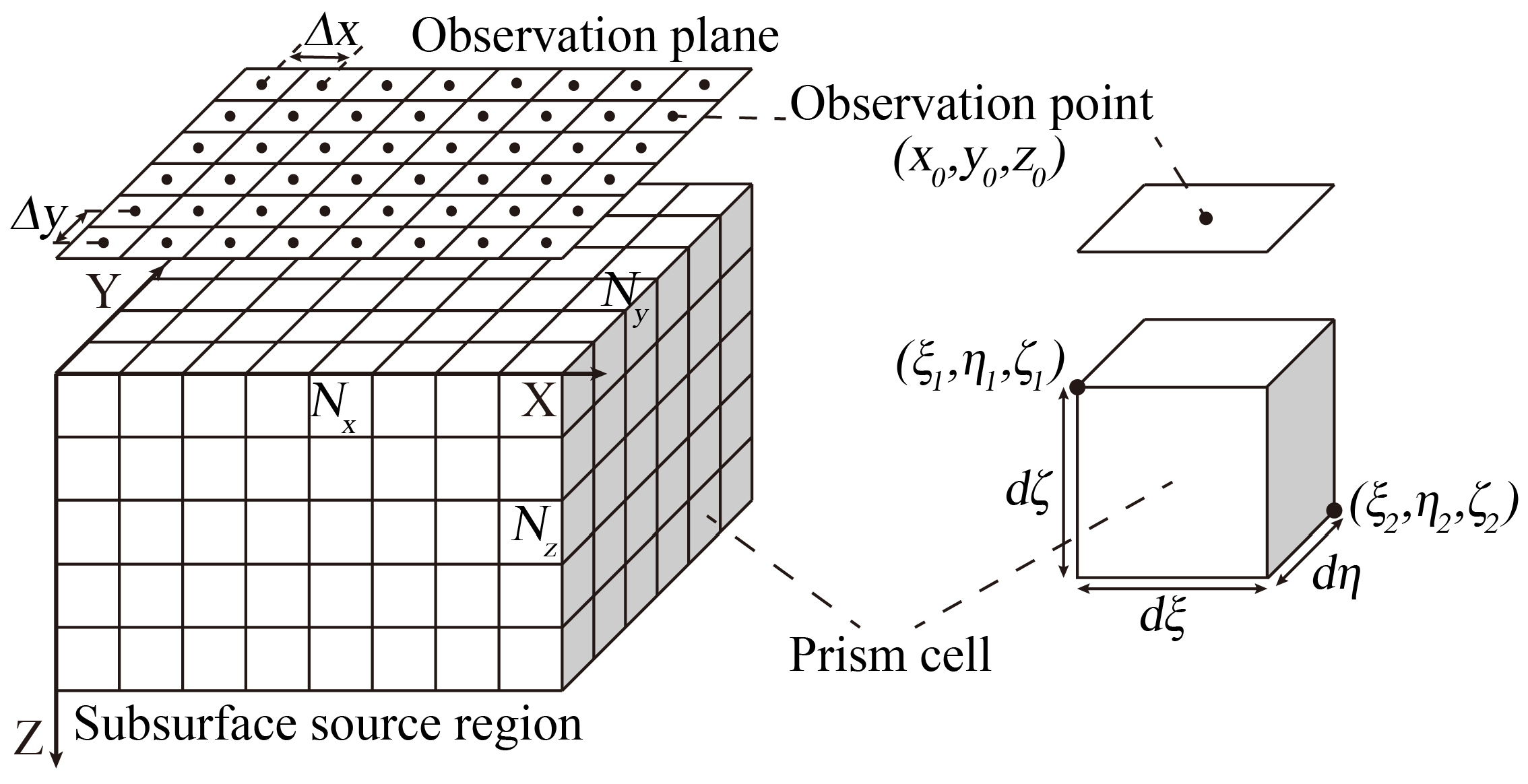
2.1. Forward Modeling

The 3-D physical property forward modeling process is shown in Figure 1. When calculating complex 3-D models, the underground field source area is divided into regular rectangular prisms at constant intervals along the x, y, and z directions. Each prism is assigned a specific density value, and the model cell density vector can be expressed as $\mathit{m}={(m_1,m_2,\dots ,m_M)}^T$, where $M=N_x\times N_y\times N_z$ represents the number of rectangular prism cells.

Consequently, through the process of gridding the observed data, all observation points are transformed onto the observation plane. This results in a one-to-one correspondence between the horizontal projection coordinates of the observation points and the coordinates of the center of the model cells. The observed data on the observation plane can be expressed as $\mathit{d}={(d_1,d_2,\dots ,d_N)}^T$, where $N=N_x\times N_y$ represents the number of observation points.

When calculating the gravity and gravity gradient anomalies generated by the aforementioned complex 3-D model, the gravity gradient anomalies produced at the observation points by all rectangular prisms in the model are summed to yield the total anomalies produced by the entire model. For a single regular prism (with the x direction from ${\xi }_1$ to ${\xi }_2$, the y direction from ${\eta }_1$ to ${\eta }_2$, and the z direction from ${\zeta }_1$ to ${\zeta }_2$) at the observation point ($x_0,y_0,z_0$), the gravity and gravity gradient anomalies are calculated as follows [28]:

$$g_z=-G_{0}m{\displaystyle \sum _{i=1}^2}{\displaystyle \sum _{j=1}^2}{\displaystyle \sum _{k=1}^2}{\mu }_{ijk}\times \left[x_{i}ln(y_j+r_{ijk})+y_{j}ln(x_i+r_{ijk})+z_{k}arctan\left({\displaystyle \frac{z_k}{r_{ijk}}}\right){\displaystyle \frac{1}{x_i{y}_j}}\right]$$

(1)

$$g_{\alpha \alpha }=G_{0}m{\displaystyle \sum _{i=1}^2}{\displaystyle \sum _{j=1}^2}{\displaystyle \sum _{k=1}^2}{\mu }_{ijk}{\displaystyle \frac{arctan\left({\beta }_j{\gamma }_k\right)}{{\alpha }_i{r}_{ijk}}}$$

(2)

$$g_{\alpha \beta }=-G_{0}m{\displaystyle \sum _{i=1}^2}{\displaystyle \sum _{j=1}^2}{\displaystyle \sum _{k=1}^2}{\mu }_{ijk}ln({\gamma }_k+r_{ijk})$$

(3)

In these equations, $G_0$ is the universal gravitational constant, and m represents the density of the prism cell. For all $\alpha ,\beta ,\gamma \in \{x,y,z\}$, the coordinates of the vertices of the prism are given by $x_i=x_0-{\xi }_i$, $y_j=y_0-{\eta }_j$, $z_k=z_0-{\zeta }_k$. Additionally, $r_{ijk}=\sqrt{x_i^2+y_j^2+z_k^2}$ and ${\mu }_{ijk}={(-1)}^{i+j+k}$.

In 3-D forward modeling, the relationship between the underground density model and the observed data is represented in matrix form as Equation (4):

$$\mathit{d}={\mathit{G}}_k\mathit{m}$$

(4)

where ${\mathit{G}}_k$ is the sensitivity matrix with dimensions ($N,M$), and $\mathit{d}$ is the observation data for a single component (such as ${\mathit{g}}_z,{\mathit{g}}_{xx},{\mathit{g}}_{xy},{\mathit{g}}_{xz},{\mathit{g}}_{yy},{\mathit{g}}_{yz},{\mathit{g}}_{zz}$). The element $G_k(i,j)$ quantitatively describes the contribution of the j-th rectangular prism cell to the observation value at the i-th observed point (where ${\mathit{G}}_k$ may represent one of the following sensitivity matrices: ${\mathit{G}}_z,{\mathit{G}}_{xx},{\mathit{G}}_{xy},{\mathit{G}}_{xz},{\mathit{G}}_{yy},{\mathit{G}}_{yz},{\mathit{G}}_{zz}$).

When data is obtained on a uniform grid, the sensitivity matrix presents a Block Toeplitz with Toeplitz Blocks (BTTB) structure [29,30]. Compressing the sensitivity matrix based on the characteristics of BTTB matrices can significantly reduce computational and storage overhead while maintaining computational accuracy, providing an effective approach for solving large-scale problems [31,32,33,34].

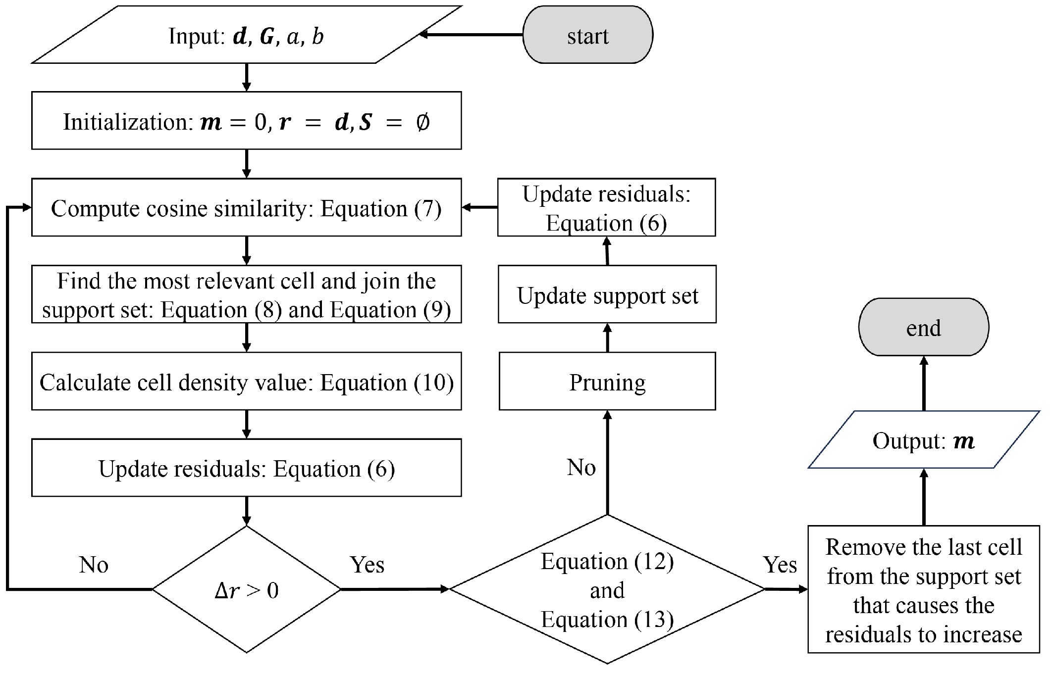
2.2. Greedy Cosine Similarity Search Algorithm (GCSSA)

The greedy algorithm is a design strategy where the core idea is to choose the locally optimal solution at each step, with the hope of accumulating local optima to reach a global optimum. This strategy was applied to mathematical optimization problems as early as the early 20th century, such as the minimum spanning tree and shortest path problems in graph theory. With the development of computer science, the greedy algorithm has been widely used in various fields, including data compression, task scheduling, resource allocation, and feature selection in machine learning [18,35,36,37,38].

In this study, the goal of the greedy algorithm is to find a sparse solution vector $\mathit{m}$, such that:

$$\mathit{d}\approx \mathit{G}\mathit{m}\left(\mathit{S}\right)$$

(5)

Here, $\mathit{d}$ denotes the combined observed data for joint inversion, $\mathit{G}$ the corresponding merged sensitivity matrix, and $\mathit{S}$ the support set. Initially, all values of the vector $\mathit{m}$ are set to zero, and the support set $\mathit{S}$ is an empty set, with the residual equal to the observation vector $\mathit{d}$. The residual is defined as Equation (6):

$$\mathit{r}=\mathit{d}-\mathit{G}\mathit{m}\left(\mathit{S}\right)$$

(6)

At each iteration, we select the cell that has the highest correlation with the current residual from the sensitivity matrix, and the cosine similarity for each model cell is calculated as Equation (7):

$$cos\left({\theta }_j\right)=cos\langle {\mathit{G}}_j,\mathit{r}\rangle ={\displaystyle \frac{{\mathit{G}}_j·\mathit{r}}{∥\mathit{r}∥∥{\mathit{G}}_j∥}}$$

(7)

where ${\mathit{G}}_j$ is the j-th column of the sensitivity matrix $\mathit{G}$, ‘·’ denotes the dot product, ‘$∥ ∥$’ represents the vector norm, and ${\theta }_j$ is the angle between the residual $\mathit{r}$ and the j-th column of the sensitivity matrix. The cosine value $cos\langle {\mathit{G}}_j,\mathit{r}\rangle$ indicates the angular similarity between the residual $\mathit{r}$ and the forward field anomaly of the j-th cell.

The index $s_j$ of the element with the highest correlation can be represented as

$$s_j=arg{\displaystyle \underset{j}{max}}[cos\left(\mathit{\theta }\right)]$$

(8)

where $\mathit{\theta }=[{\theta }_1,{\theta }_2,\dots ,{\theta }_M]$, M is the number of cells, and arg denotes the index of the cell with the highest correlation. After identifying the most relevant cell, this cell is added to the support set:

$$\mathit{S}={\mathit{S}}_{\mathrm{pre}}\cup \left\{s_j\right\}$$

(9)

where $\mathit{S}$ is the updated support set, ${\mathit{S}}_{\mathrm{pre}}$ is the previous support set, and $s_j$ is the set containing the element with the highest correlation.

Once the most relevant cell is determined, the density value of the cell must also be established. The prior information sets the density constraints to $[a,b]$, where a is a positive constraint and b is a negative constraint. If all densities are positive, then $b=0$; if all densities are negative, then $a=0$. The density value ${\rho }_j$ of the currently relevant cell is given by:

$${\rho }_j=\left\{\begin{array}{cc}a\hfill & \mathrm{if}cos\left({\theta }_j\right)>0\hfill \\ b\hfill & \mathrm{if}cos\left({\theta }_j\right)<0\hfill \end{array}\right.$$

(10)

The density is assigned to the solution vector $\mathit{m}$ at the current most relevant element $s_j$:

$$\mathit{m}\left(s_j\right)={\rho }_j$$

(11)

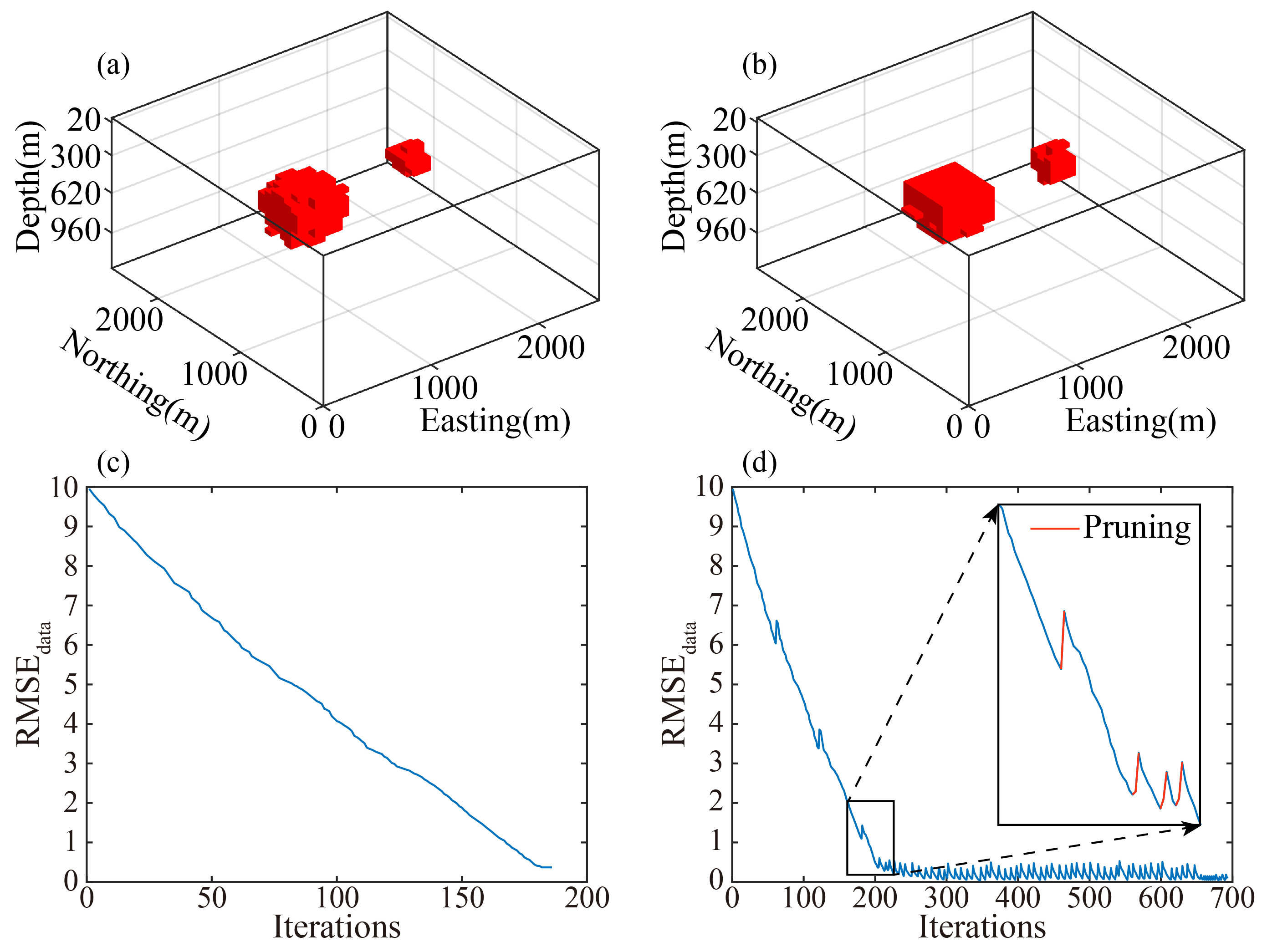
2.3. Pruning Mechanism

In the process of sparse inversion, due to the underdetermined nature and non-uniqueness of the gravity inverse problem, greedy search methods are prone to selecting incorrect cells when identifying the most correlated basis elements. Once these erroneous cells are added to the support set, they may distort the residual structure and lead to a chain of adverse effects, including false density compensation of opposite sign, spatially dispersed model elements, and blurred geological boundaries. To suppress such cumulative errors, this study incorporates a pruning mechanism into the greedy cosine similarity-based inversion algorithm, thereby enhancing the accuracy of support set construction and the overall robustness of the inversion model.

The core idea of this mechanism is to identify and remove potentially misselected cells from the support set, enabling the algorithm to backtrack and search for better candidates. Specifically, the pruning strategy focuses on four types of anomalous cells.

1.

Cells exhibiting excessively large or small projection amplitudes on the residuals, which typically indicate overestimation or underestimation of depth;

2.

Cells whose addition results in an increased residual norm, suggesting that they do not contribute to convergence and are likely misclassified;

3.

Cells already included in the support set that exhibit high similarity to the current residuals but possess an opposite density sign, often reflecting previously selected compensation errors that may induce residual oscillations;

4.

Spatially isolated cells that do not form part of a continuous geological structure, which are likely caused by noise and lack physical plausibility.

The pruning mechanism includes both scheduled activation after a fixed number of iterations and dynamic activation triggered when the addition of a new cell leads to an increase in the residual.

Once activated, the algorithm enters the pruning module, which evaluates all units in the current support set based on the aforementioned criteria and removes those that meet the pruning conditions. After pruning, the residual is updated, and the algorithm re-initiates the search for new candidate units. This mechanism introduces a form of self-correction within the greedy search framework, enabling the early elimination of misselected units before significant error propagation occurs. As a result, it effectively limits unnecessary support set expansion and enhances the robustness and reliability of convergence of the inversion.

Once the pruning mechanism is introduced, the composition of the support set may fluctuate dynamically due to the iterative removal and re-selection of candidate cells. To ensure a reliable termination of the inversion process, we propose a comprehensive convergence criterion that jointly considers both structural stability and data misfit.

First, the structural stability of the support set is assessed by computing the Jaccard similarity index between the support sets before two consecutive pruning events. If the Jaccard index exceeds a threshold of 0.99, the structure of the support set is considered to have stabilized. Second, the data misfit is evaluated by monitoring the change in the residual norm. If the absolute difference between the residual norms of two successive iterations falls below a predefined threshold $\epsilon$ (e.g., 0.001), it is inferred that further updates yield negligible improvements in data fitting.

$$\mathrm{Jac}({\mathit{S}}^{\left(k\right)},{\mathit{S}}^{(k-1)})={\displaystyle \frac{|{\mathit{S}}^{\left(k\right)}\cap {\mathit{S}}^{(k-1)}|}{|{\mathit{S}}^{\left(k\right)}\cup {\mathit{S}}^{(k-1)}|}}$$

(12)

$$\left|\parallel {\mathit{r}}^{\left(k\right)}{\parallel }_2-{\parallel {\mathit{r}}^{(k-1)}\parallel }_2\right|<\epsilon$$

(13)

Here, k denotes the number of times the pruning mechanism is triggered. To improve the robustness of the convergence judgment, one can further require that both criteria be satisfied a certain number of times (e.g., twice) before the inversion is declared fully converged.

Figure 2 illustrates the complete inversion workflow with the integrated pruning mechanism. The pruning module is dynamically activated after each residual update to continuously evaluate the rationality of the current support set and to mitigate the risk of convergence to suboptimal solutions.

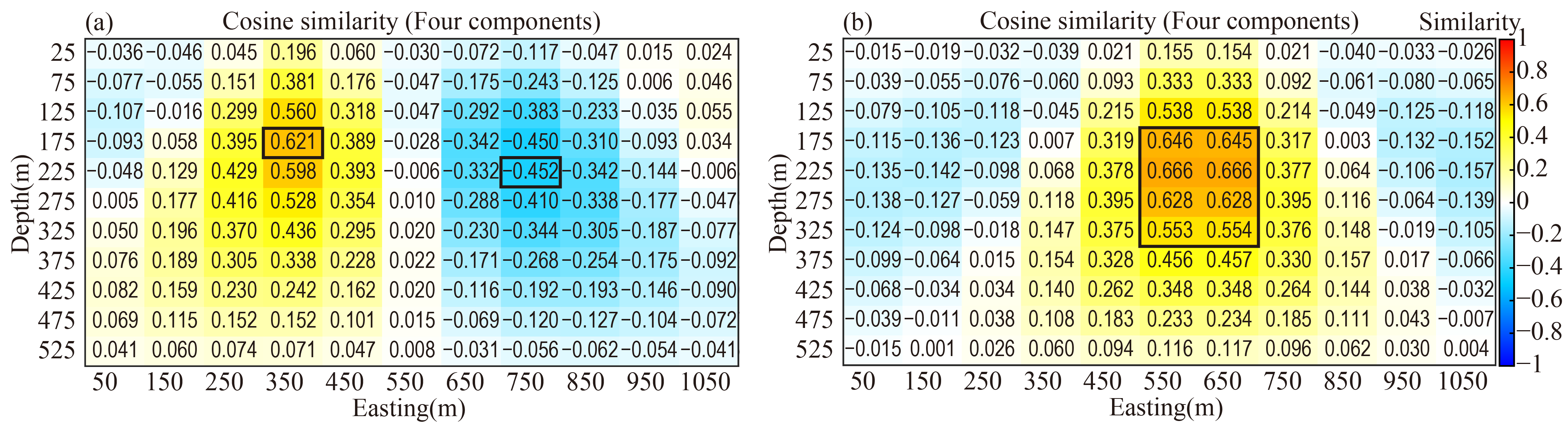
2.4. Related Cell Searches for Cosine Similarity in Joint Gravity and Gravity Gradient Data

To validate the effectiveness of cosine similarity as a metric for identifying model cells most correlated with gravity and gravity gradient anomalies, this section presents three forward-model-based illustrative examples. It is important to note that these examples are not intended to demonstrate final inversion results, but rather to theoretically evaluate the spatial indication capability of cosine similarity as a search function in the inversion process. Full inversion procedures and results are discussed in Section 3.

In contrast, the cosine similarity-based approach [39,40] used in this study evaluates the correlation between each model cell and the observed data solely based on the angular similarity between the field residual vector and the sensitivity response vector of each cell, without regard to their magnitudes. This formulation inherently reduces the influence of amplitude and unit discrepancies between gravity and gravity gradient data.

In the first example, a model consisting of a single cell is used to generate gravity and gravity gradient anomalies at the surface (Figure 3a), with the model configuration shown in Figure 3b. The cosine similarities between the forward responses and the residual data are computed both for individual anomaly components and for their joint combination. As shown in Figure 3c–g, the spatial location corresponding to the highest cosine similarity closely matches the actual position of the model cell, confirming that both individual components and multi-component combinations are effective in identifying the most relevant regions using cosine similarity.

The second example involves a two-cell model with contrasting density signs and different burial depths. As illustrated in Figure 4a–c, the cosine similarity analysis still successfully pinpoints the positively and negatively correlated regions. This demonstrates that the method is capable of reliably detecting both positive and negative density anomalies. Since cosine similarity effectively measures the angular alignment between the observed data vector $\mathit{d}$ and each column of the sensitivity matrix $\mathit{G}$, it can be interpreted as evaluating the spatial similarity of each cell’s unit-density-induced field. In this context, a negative cosine value naturally corresponds to an anomaly generated by a negative density contrast.

The third example examines a more complex target composed of eight cells. The forward-modeled surface anomaly is shown in Figure 4d, and the corresponding model configuration is presented in Figure 4e. The resulting cosine similarity distribution (Figure 4f) shows that the highest values are concentrated exactly at the locations of the eight model cells, confirming that cosine similarity remains a robust indicator even for composite anomalies.

These examples collectively validate the effectiveness and interpretability of cosine similarity as a reliable search metric for guiding sparse inversion.

Additionally, the analysis indicates that cosine similarity values remain relatively high across a range of depths associated with relevant model cells. This is particularly evident for deeper cells, due to the intrinsic decay characteristics of the sensitivity matrices: gravity and gravity gradient responses decrease approximately with ${\mathit{z}}^{-2}$ and ${\mathit{z}}^{-3}$, respectively. As depth increases, the induced anomaly variations from a given cell become less distinguishable, leading to smaller changes in the correlation measure.

This property may result in an overestimation of the depth contribution in practical inversions. To address this, a depth attenuation function is introduced to moderately suppress the similarity values of deeper cells. Specifically, a quadratic decay function is employed, as defined in Equation (14), to penalize correlations from cells at greater depths and improve inversion reliability.

$$\mathit{W}z={\displaystyle \frac{-{\mathit{z}}^2}{H^2}}+1$$

(14)

where $\mathit{z}$ denotes the depth of the cell’s center and H is the maximum depth of the field source area.

After applying the depth attenuation function, the cosine similarity distribution becomes more balanced with respect to depth. As shown in Figure 5, the overestimation of deep units is effectively suppressed.

3. Numerical Modeling Experiments and Analysis

To validate the effectiveness of the proposed algorithm in complex geological scenarios, two sets of synthetic model experiments were carried out. Through step-by-step analyses involving noise tests, data combination experiments, and comparative evaluations with conventional methods, the feasibility and stability of the algorithm were comprehensively demonstrated.

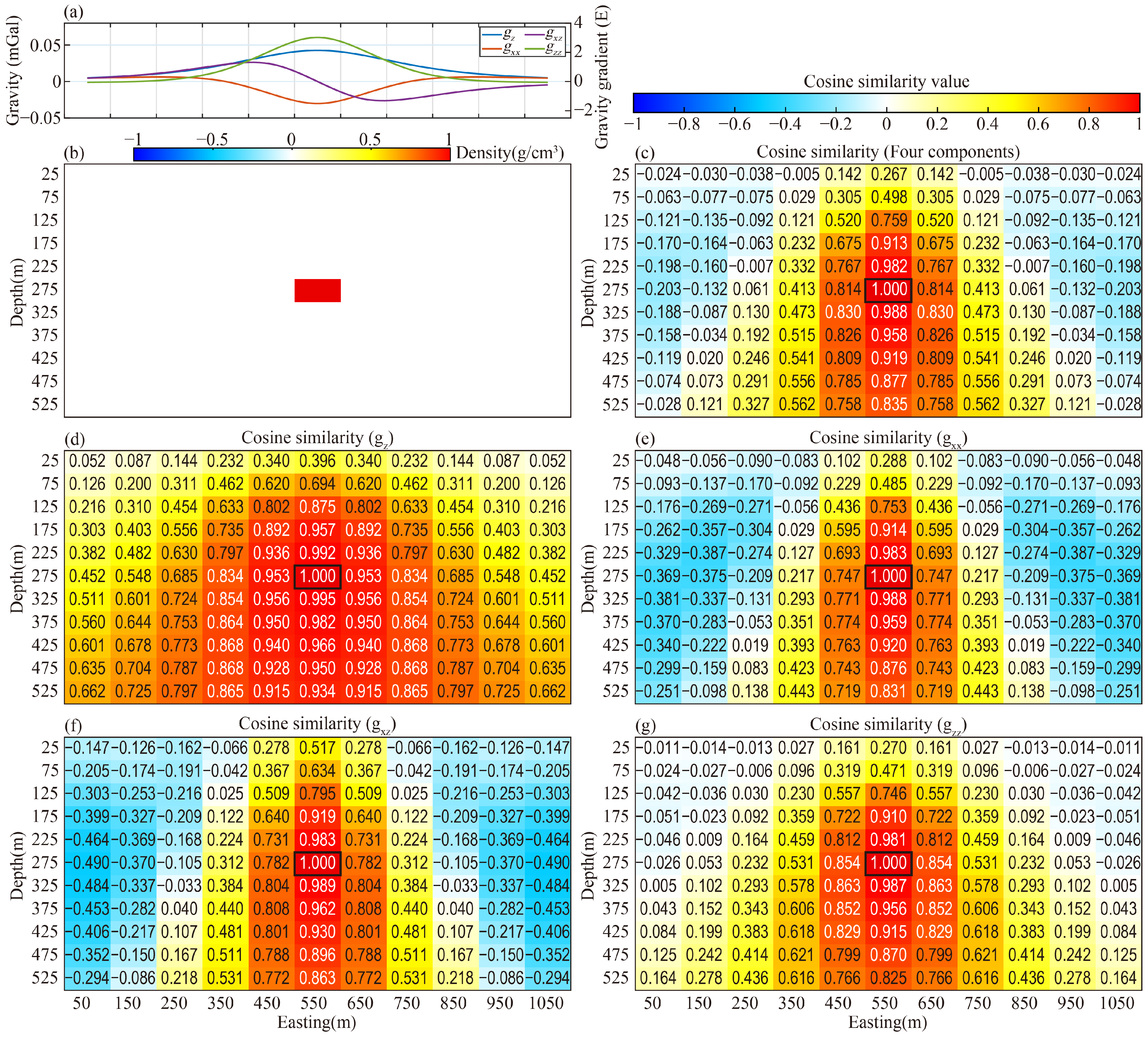
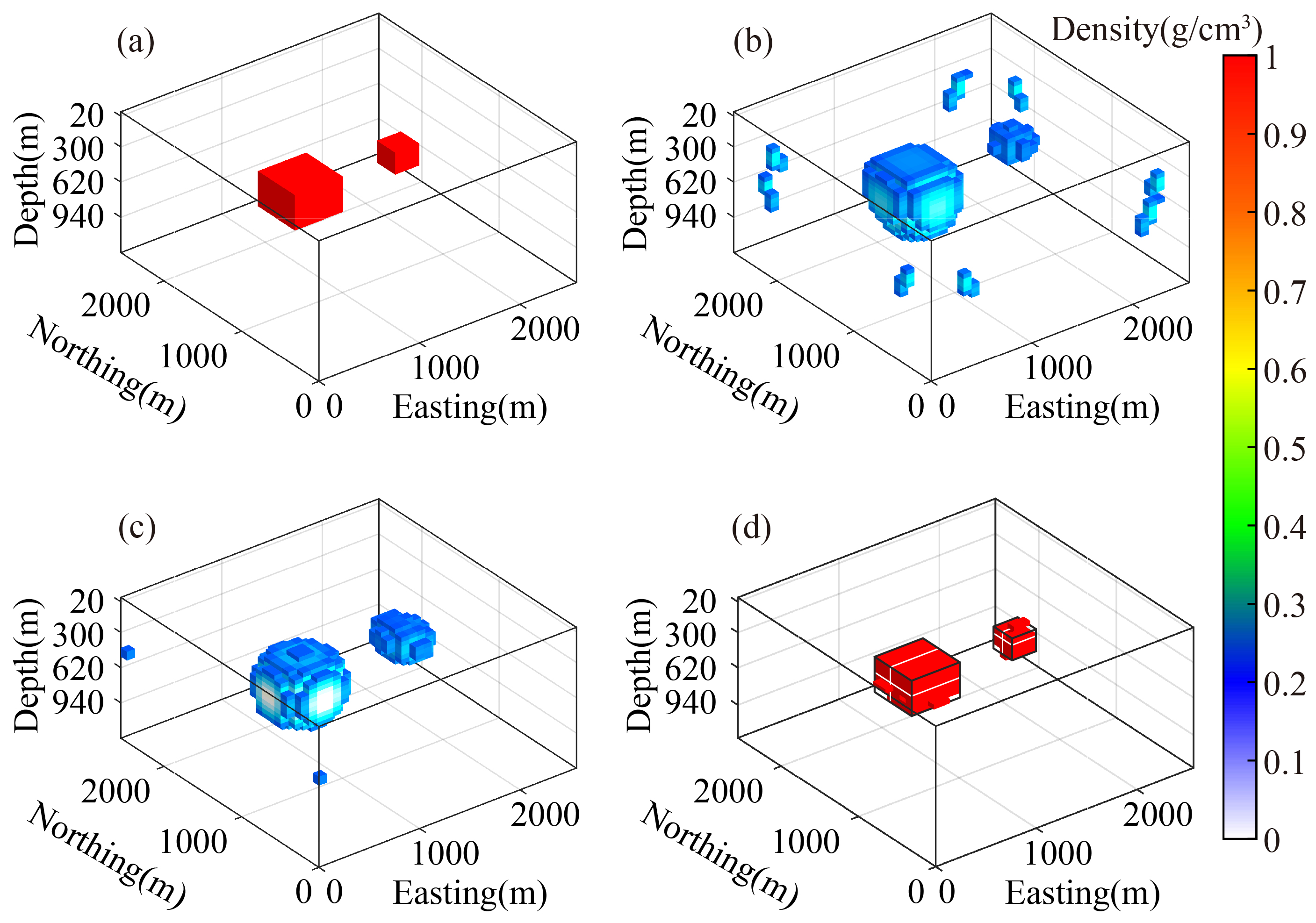
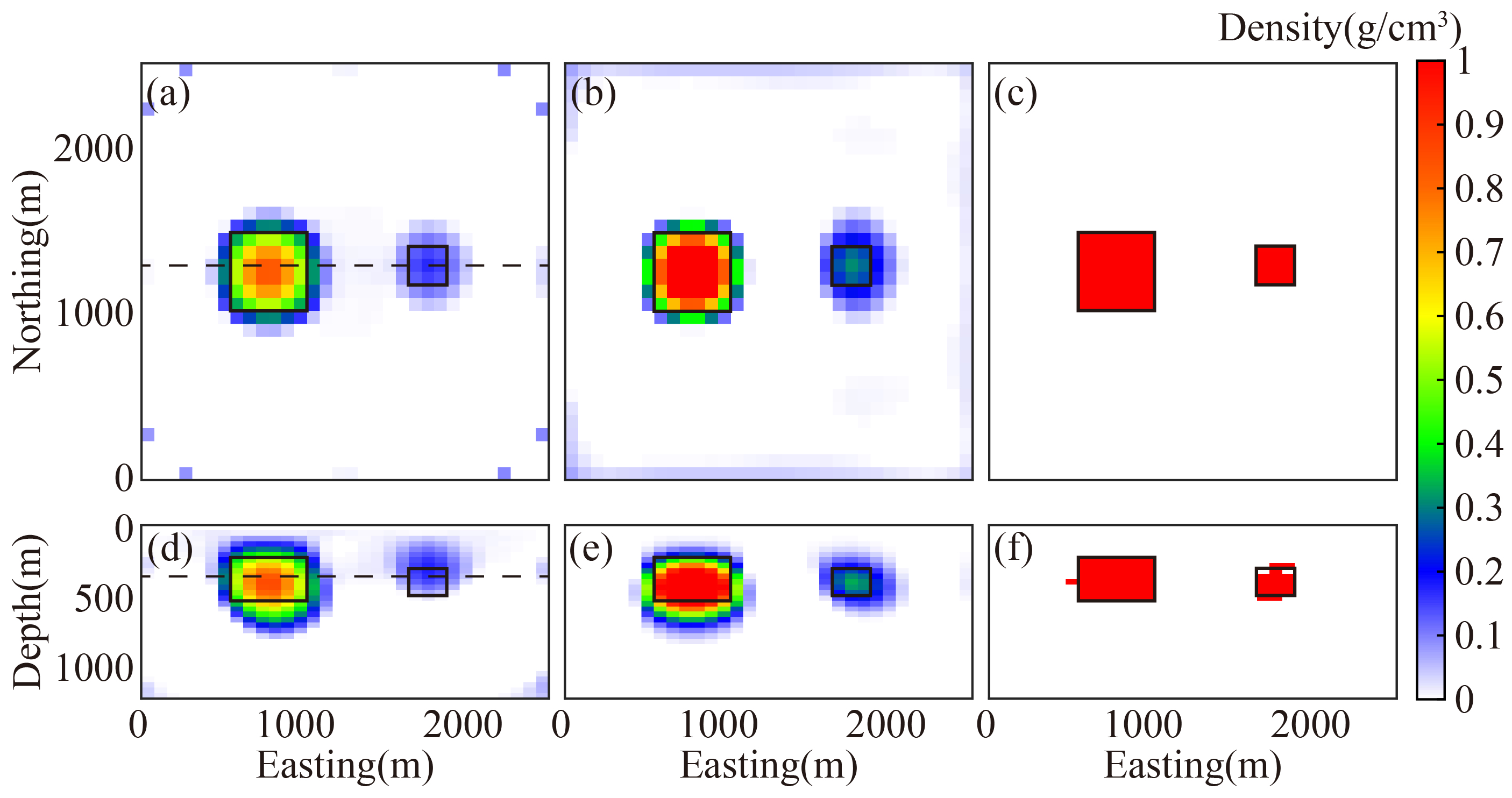
3.1. Feasibility Verification with a Simple Synthetic Model

To evaluate the effectiveness of the proposed pruning mechanism and the overall performance of our inversion method compared to existing approaches, we first designed a synthetic model comprising two density anomalies of different sizes.

The source grid spans a volume of (0–2560 m, 0–2560 m, 0–1280 m), corresponding respectively to the east–west (x-axis), north–south (y-axis), and vertical (z-axis) directions. The model includes a larger and a smaller block. The larger anomaly occupies the range (560–1040 m, 1040–1520 m, 240–560 m), while the smaller anomaly is located within the range (1680–1970 m, 1200–1440 m, 320–520 m).

The source region is discretized into a 32 × 32 × 32 grid of rectangular prisms. Synthetic observation data are generated at the horizontal projection of the center of each cell, yielding 32 × 32 surface data points. The forward modeling results are illustrated in Figure 6, where the anomaly caused by the smaller block is barely visible to the naked eye, making it a challenging target for inversion.

To assess the role of pruning in inversion performance, we first conducted a comparative experiment with and without the pruning mechanism. Figure 7a,b present the 3D inversion results for both cases using gravity ($g_z$) and full tensor gravity gradient (6C) data, respectively, where 6C represents the full tensor gravity gradient data consisting of $g_{xx}$, $g_{xy}$, $g_{xz}$, $g_{yy}$, $g_{yz}$, and $g_{zz}$. Figure 7c,d show the corresponding root-mean-square error curves for data misfit (RMSE_data) over iterations.

Without the pruning mechanism, the inversion fails to fully delineate the boundaries of the anomalies. Several relevant cells, particularly those at the edges, are missed, and the RMSE_data curve exhibits signs of stagnation, indicating a lack of convergence. In contrast, the inclusion of pruning significantly improves boundary recovery and model accuracy. The RMSE_data curve in this case shows multiple pruning events followed by stabilization, suggesting improved convergence and reliability.

A quantitative evaluation further highlights the benefits of the pruning mechanism. Without pruning, the inversion correctly identifies 288 anomaly cells, with 63 false positives. The model misfit RMSE_model is 0.0574, the mean absolute error (MAE) is 0.003296, and the Pearson correlation coefficient (PCC) between the true and inverted models is 0.840738. After applying pruning, the number of correctly recovered cells increases to 321, with only 10 false positives. The RMSE_model drops to 0.0259, the MAE to 0.000671, and the correlation coefficient improves to 0.966533. These results confirm that pruning enhances both inversion accuracy and convergence behavior.

$${\mathrm{RMSE}}_{\mathrm{data}}=\sqrt{{\displaystyle \frac{1}{n}}\sum _{i=1}^n{(d_i^{\mathrm{obs}}-d_i^{\mathrm{pred}})}^2}$$

(15)

$${\mathrm{RMSE}}_{\mathrm{model}}=\sqrt{{\displaystyle \frac{1}{M}}\sum _{j=1}^M{(m_j^{\mathrm{true}}-m_j^{\mathrm{inv}})}^2}$$

(16)

$$\mathrm{MAE}={\displaystyle \frac{1}{M}}{\displaystyle \sum _{j=1}^M}\left|m_j^{\mathrm{true}}-m_j^{\mathrm{inv}}\right|$$

(17)

$$\mathrm{PCC}={\displaystyle \frac{{\sum }_{j=1}^M(m_j^{\mathrm{true}}-{\overline{m}}^{\mathrm{true}})(m_j^{\mathrm{inv}}-{\overline{m}}^{\mathrm{inv}})}{\sqrt{{\sum }_{j=1}^M{(m_j^{\mathrm{true}}-{\overline{m}}^{\mathrm{true}})}^2{\sum }_{j=1}^M{(m_j^{\mathrm{inv}}-{\overline{m}}^{\mathrm{inv}})}^2}}}$$

(18)

where n is the total number of data points used in the joint inversion, ${\mathit{d}}^{\mathrm{obs}}$ is the observed data, ${\mathit{d}}^{\mathrm{pred}}$ is the predicted data from the inversion result, ${\mathit{m}}^{\mathrm{true}}$ is the true model, ${\mathit{m}}^{\mathrm{inv}}$ is the inverted model, and $\overline{m}$ denotes the mean value.

To further validate our method, we compare it against two commonly used inversion approaches. The conventional L₂-norm inversion method follows the framework of Li and Oldenburg [11], without employing logarithmic constraints. For model weighting, we combine the depth weighting function ${\mathit{W}}_z$ [41] with the model integral sensitivity matrix $\mathit{S}=\mathrm{diag}\left(\sqrt{{\mathit{G}}^T\mathit{G}}\right)$ [10,42], resulting in the weighting matrix ${\mathit{W}}_m={\mathit{W}}_z\mathit{S}$. This approach provides consistent sensitivity compensation without introducing subjective smoothing weights [10,41]. The objective function is minimized using the Gauss–Newton method with a preconditioned conjugate gradient (PCG) solver. The PCG iterations terminate when the relative residual falls below ${10}^{-2}$, and the Gauss–Newton iterations stop when the relative change in the objective function satisfies ${\displaystyle \frac{|{\varphi }^n-{\varphi }^{n-1}|}{|{\varphi }^n|}}<{10}^{-3}$. A Jacobi-like preconditioner with $\mathit{M}=\mathrm{diag}\left(\mathit{A}\right)$ is applied. The second uses the SL0 regularization algorithm proposed by Niu et al. [7]. For the SL0 inversion method, we adopt the empirically recommended parameters and convergence criteria as suggested by the original authors. The depth weighting function’s upper and lower boundaries are set according to the actual depths corresponding to the models in this study. All methods are constrained with the same density bounds [0, 1] for fairness. Figure 8a shows the 3D view of the true model, while Figure 8b–d present the inversion results from each method.

As seen from the 3D results, all three methods successfully localize the two anomalies and differentiate their sizes. To enable more detailed comparison, horizontal and vertical slices through the models are presented in Figure 9. The vertical slice is taken at 1320 m along the north direction, and the horizontal slice at 380 m depth. Their positions are indicated with white lines in Figure 8d and with dashed lines in Figure 9a,d.

The L₂-norm regularization method yields smooth and diffuse results, with underestimated density values. The SL0 method improves upon this, producing more compact anomalies with better density estimates. However, the proposed method outperforms both, yielding sharp and accurate boundaries.

These results demonstrate that the proposed inversion method not only achieves superior resolution and convergence with the inclusion of the pruning mechanism but also avoids being trapped in suboptimal solutions associated with large anomalies. It is capable of accurately resolving both large and small model blocks, making it a robust approach for practical applications involving targets of varying scales.

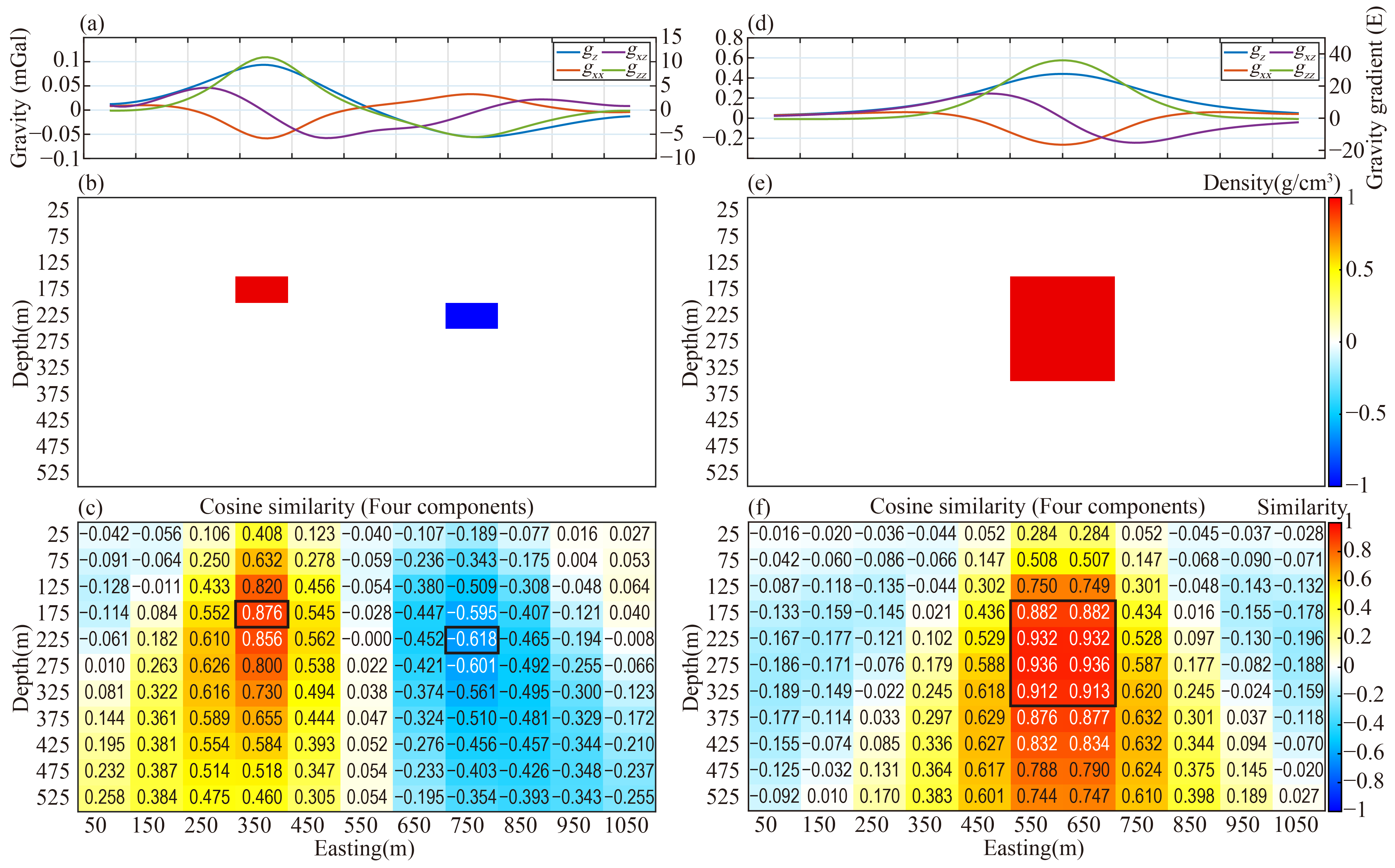
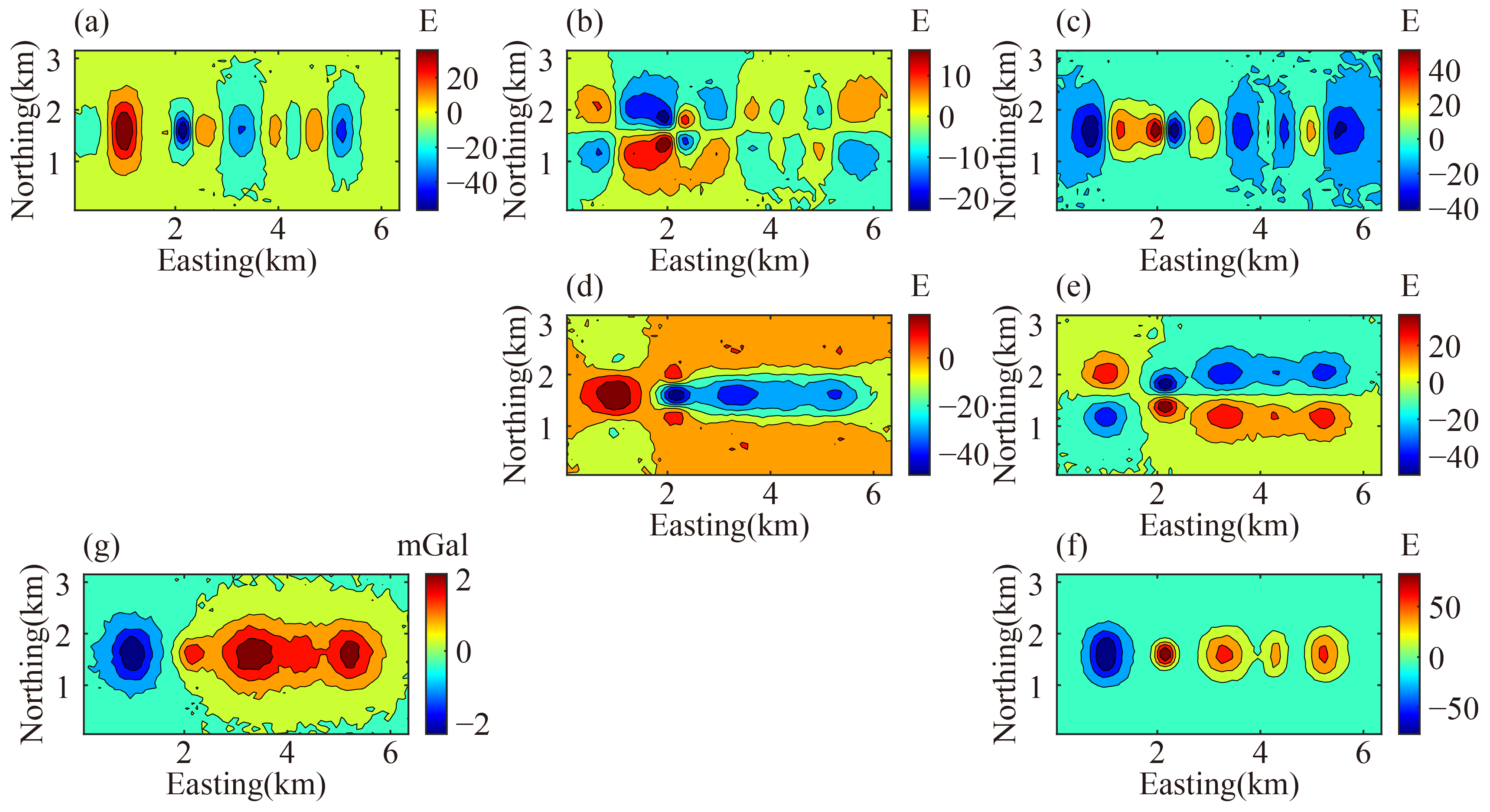
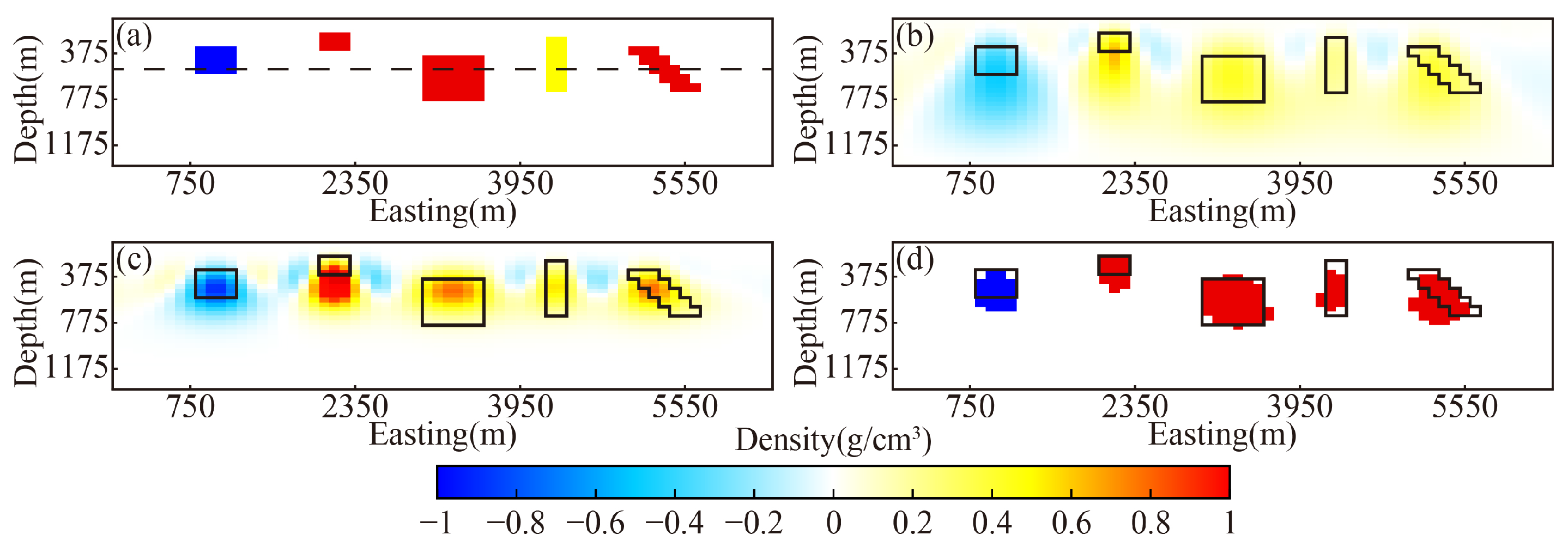
3.2. Robustness and Multi-Component Performance Evaluation with a Complex Model

While the greedy algorithm performs well in recovering simple sparse solutions, real geological scenarios are often more complex. To test the proposed method under such conditions, we designed a synthetic model with multiple anomaly bodies considering mainly positive density contrasts while deliberately including one structure with a negative contrast (model block 1), small shallow targets (model block 2), large deep-seated structures (model block 3), vertically elongated bodies with moderately high density below the assumed upper bound (model block 4), and dipping dike anomalies representing challenging cases (model block 5). Each block differs in size, shape, and depth, and the detailed parameters are listed in

Table 1. Range and density of model blocks in each dimension.

Model Blocks 1	Eastward Range (m)	Northward Range (m)	Depth Range (m)	Density (g/cm3)
Model block 1	800–1200	1200–2000	300–600	−1
Model block 2	2000–2300	1400–1800	150–350	1
Model block 3	3000–3600	1300–1900	400–900	1
Model block 4	4200–4400	1200–2000	200–800	0.5
2 Model block 5	5000–5700	1200–2000	300–800	1

¹ The numbering sequence of the model blocks is increasing along the eastward. ² Each step is 100 m thick in the depth direction and increases by 100 m in the east direction for each step block as the depth increases.

. This setup enables us to comprehensively assess the algorithm’s ability to reconstruct multiple complex targets. The extended model covers a larger area of (0–6400 m, 0–3200 m, 0–1600 m), discretized into 64 × 32 × 32 cells, with 64 × 32 observation points.

To examine the robustness of the proposed method, we conducted a series of noise experiments by adding Gaussian noise at varying levels to the synthetic data. This noise level is based on the standard deviation of the original data. The inversion accuracy under different noise conditions was quantitatively evaluated using the RMSE_model, MAE, and the PCC between the true and inverted density models. As summarized in

Table 2. Inversion performance of the proposed method under different Gaussian noise levels: RMSE_model, MAE, and PCC.

Noise Levels 1	0%	1%	2%	5%	10%	15%	20%	35%
RMSEmodel(×${10}^{-2}$)	7.97	8.11	8.13	8.17	8.20	8.26	8.37	8.41
MAE(×${10}^{-3}$)	7.08	7.31	7.34	7.40	7.46	7.55	7.74	7.80
PCC	0.768	0.759	0.758	0.757	0.754	0.749	0.743	0.736

¹ This noise level is based on the standard deviation of the original data.

, the proposed method maintains high inversion quality when the noise level is below 10%, successfully capturing the geometry and boundaries of the anomaly bodies. However, as the noise increases to 15% or higher, the results begin to deteriorate, with reduced resolution and increased deviation. Therefore, we selected the 10% noise level as a representative condition for subsequent evaluations. The noise-contaminated observations corresponding to the 10% noise level are shown in Figure 10.

Building upon the 10% noise scenario, we further investigated the impact of different data combinations on inversion performance. Specifically, we tested four cases: (1) single-component inversion using either gravity or one gravity gradient component, (2) joint inversion of $g_z$ and the $g_{zz}$ component, (3) inversion using the full tensor of gravity gradient (6C) data, and (4) joint inversion incorporating both $g_z$ and 6C. The comparative results are listed in

Table 3. Comparison of inversion performance using single-component and joint inversion.

	${\mathit{g}}_{\mathit{z}}$	${\mathit{g}}_{\mathit{xx}}$	${\mathit{g}}_{\mathit{xy}}$	${\mathit{g}}_{\mathit{xz}}$	${\mathit{g}}_{\mathit{yy}}$	${\mathit{g}}_{\mathit{yz}}$	${\mathit{g}}_{\mathit{zz}}$	${\mathit{g}}_{\mathit{z}}$ & ${\mathit{g}}_{\mathit{zz}}$	6C	${\mathit{g}}_{\mathit{z}}$ & 6C
RMSEmodel (×${10}^{-1}$)	1.10	0.979	0.951	0.898	1.12	1.07	0.830	0.828	0.820	0.813
MAE (×${10}^{-2}$)	1.28	1.03	0.98	0.88	1.32	1.22	0.76	0.75	0.74	0.73
PCC	0.5563	0.6248	0.6654	0.6974	0.5479	0.5876	0.7479	0.7497	0.7535	0.7569

. It can be observed that joint inversion consistently outperforms single-component inversion in terms of RMSE_model, MAE, and correlation with the true model. In particular, the comprehensive use of $g_z$ and 6C data provides the most accurate and stable inversion results, highlighting the advantages of multi-component data integration.

Finally, under the 10% noise condition, we compared the inversion performance of the proposed method with two conventional algorithms: L₂-norm regularization and SL0 regularization. All three methods employed the same density bounds of [−1, 1]. Figure 11a is a three-dimensional view of the True model. The corresponding 3D inversion results are displayed in Figure 11b–d. Among the three methods, the proposed approach produces the most compact anomalies with sharp boundaries, closely matching the true model configuration.

To gain further insight into the spatial accuracy, horizontal and vertical slices were extracted from the inverted models, as shown in Figure 12 and Figure 13. The slices were taken at 1550 m north and 525 m depth, respectively, with their positions marked in Figure 12a and Figure 13a. The conventional L₂-norm inversion can roughly indicate the anomaly positions and polarities, but suffers from excessive smoothing and poor boundary delineation. The SL0 approach improves compactness and boundary clarity, yet still shows certain smoothing effects. In contrast, the proposed method yields accurate, well-bounded reconstructions that are robust to noise interference, and effectively overcomes challenges in selecting model constraints, depth weighting functions, and inversion parameters, and thus exhibits clear advantages in resolving complex underground structures.

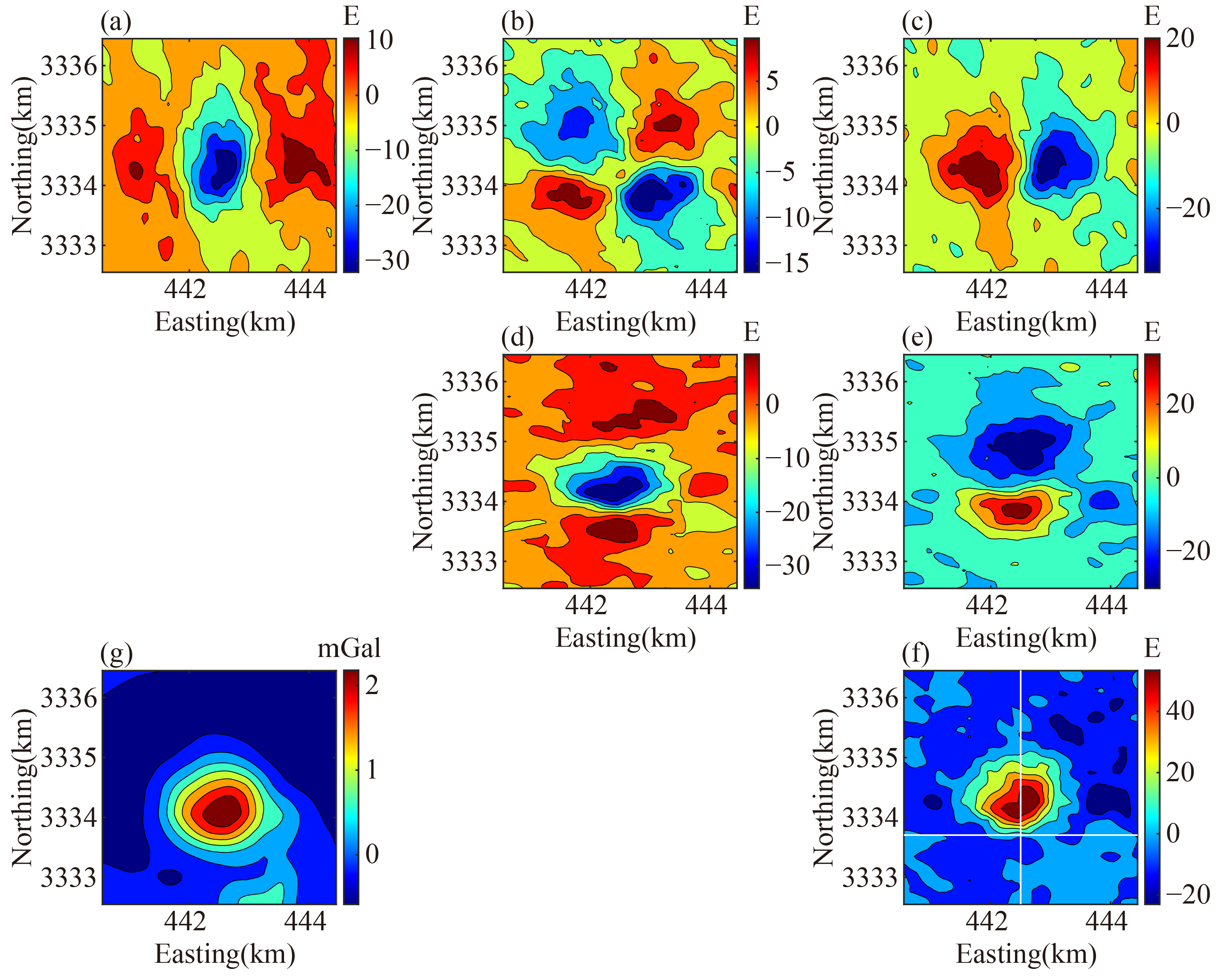
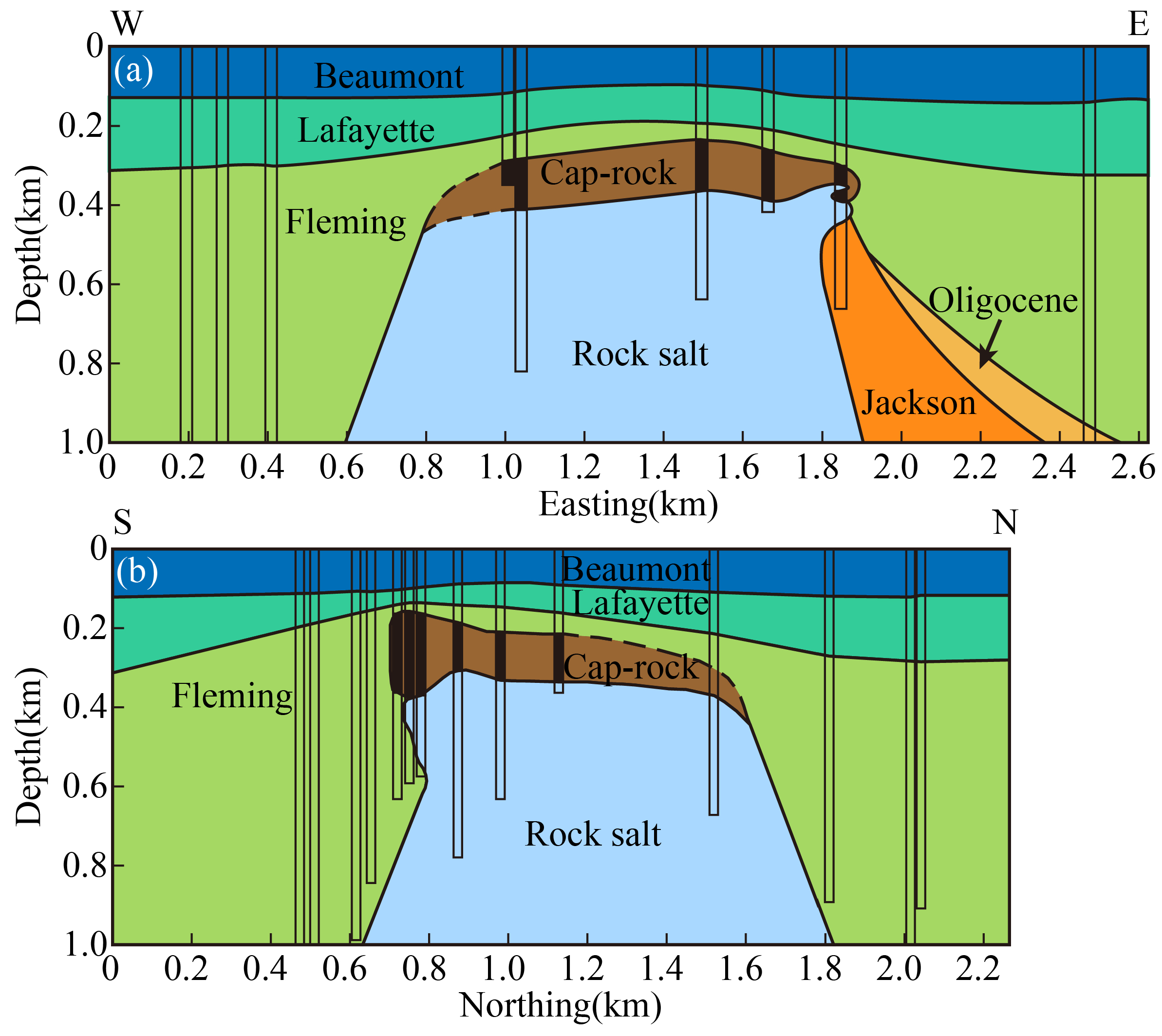
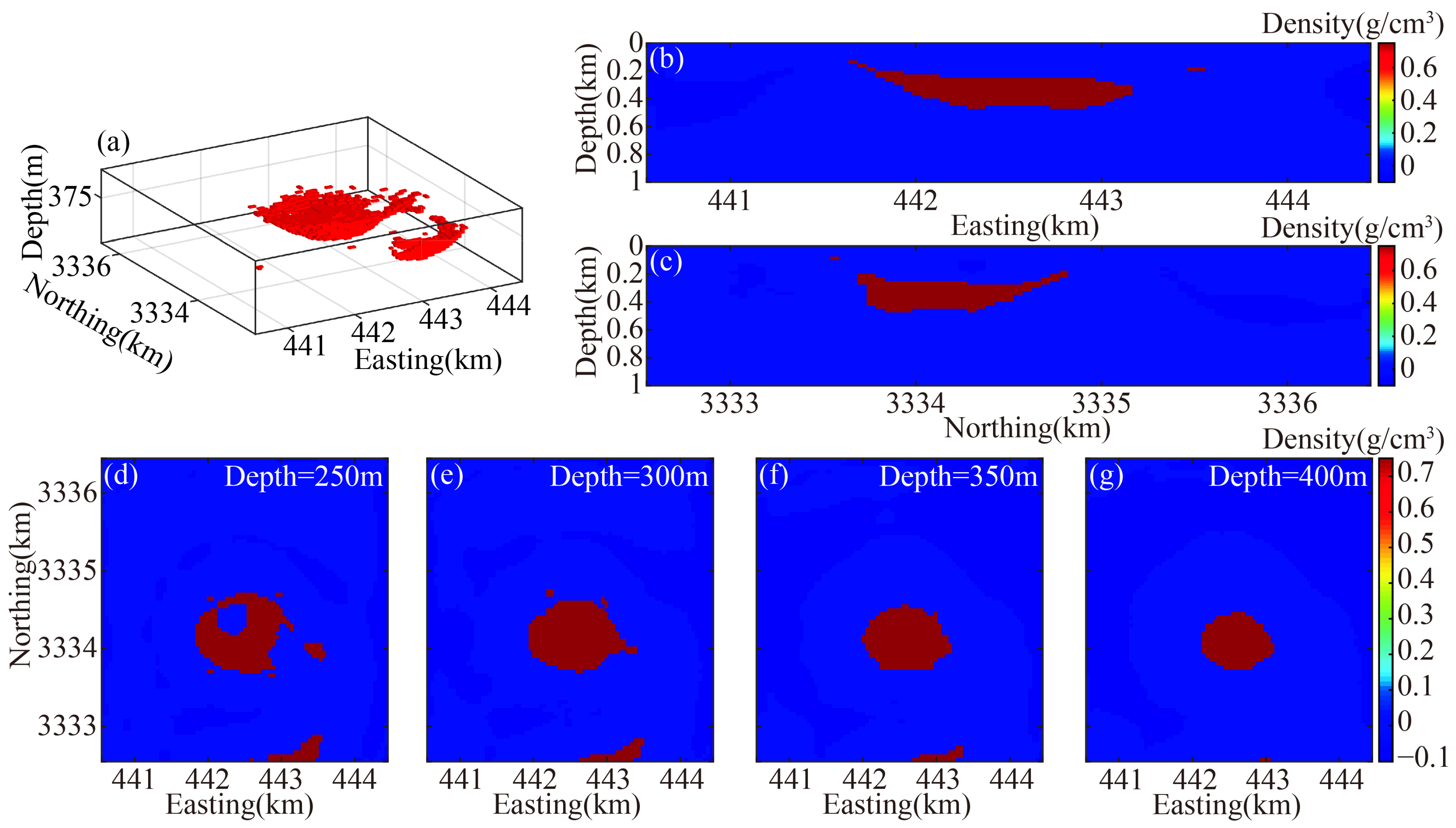
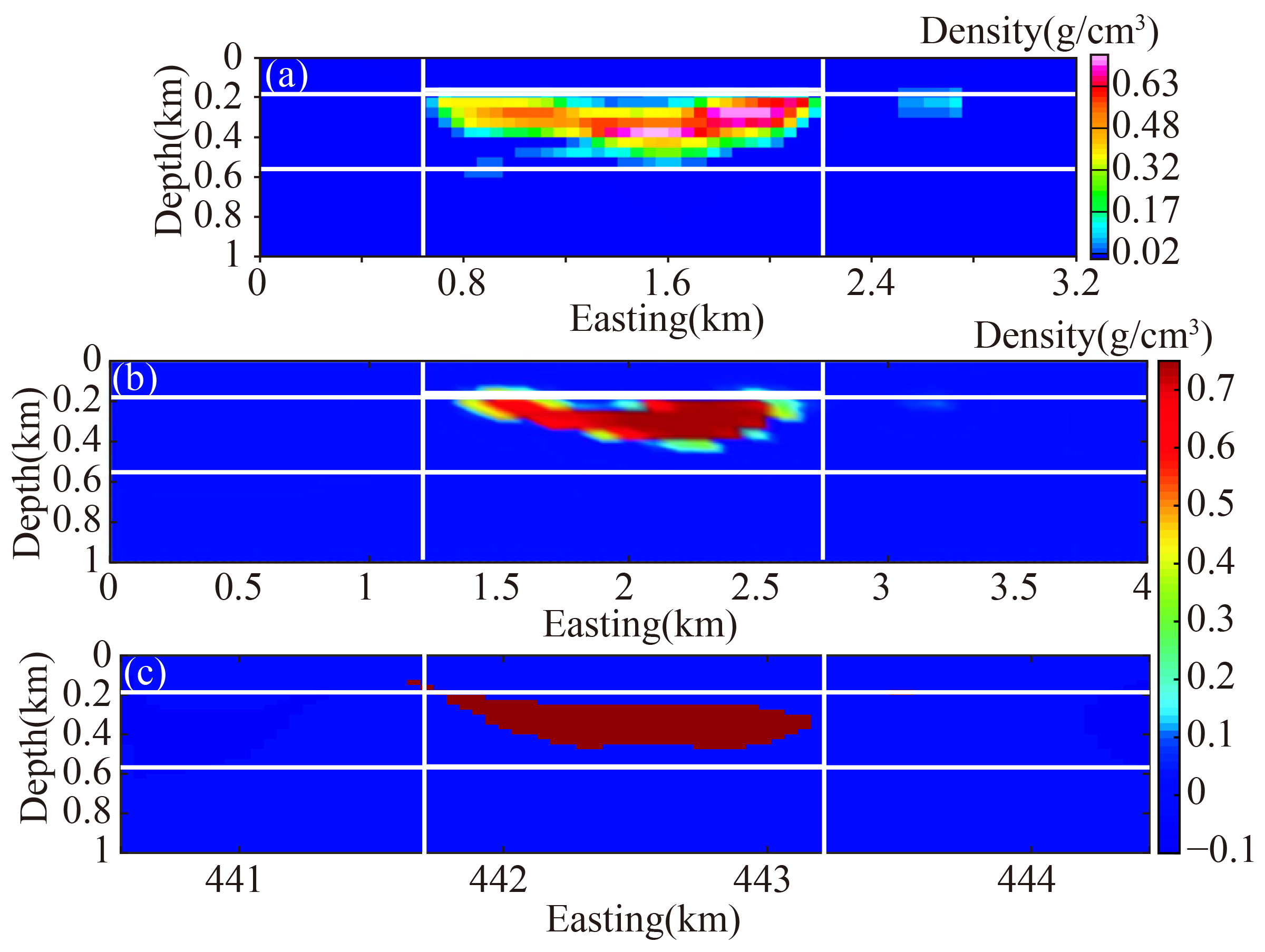
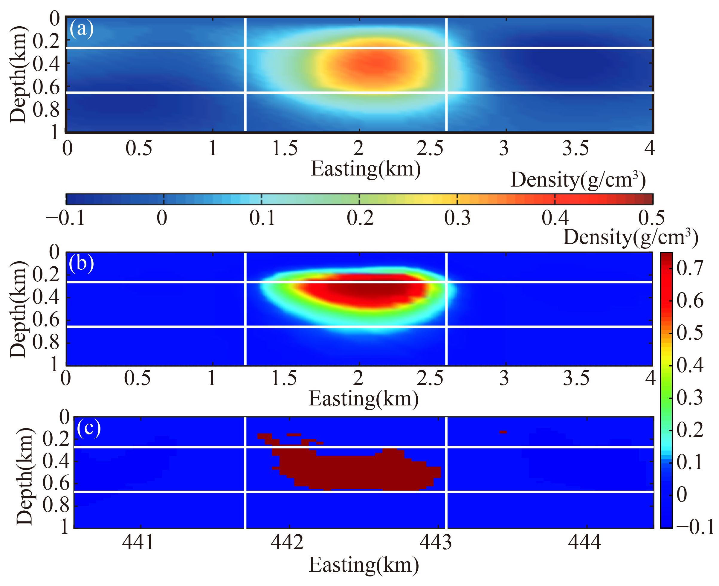
4. Application to Real Data

In this section, we employ ground gravity data and airborne full-tensor gravity gradient (FTG) data from the Vinton Salt Dome region to substantiate the efficacy of the proposed inversion methodology under real data conditions. The Vinton Salt Dome, located in Southwestern Louisiana, USA, is a diapiric structure intimately associated with significant oil and gas accumulations. It comprises a nearly block-shaped salt core and a distinctive overlying caprock, forming a classic salt diapir morphology. This includes an interior salt body, an overlying caprock composed mainly of limestone, gypsum, and anhydrite with a density of approximately 2.75 g/cm³, and deformed sedimentary flanks. Due to the marked density contrast between the salt and surrounding sediments, gravity and gravity gradient methods are well-suited for delineating the salt dome.

The structural complexity of the Vinton Dome poses inherent inversion challenges. Shallow caprocks often undergo dehydration and densification processes, forming high-density gypsum layers above the salt structure. In addition, undulations in the sedimentary background interfaces contribute significant gravity signals, complicating the isolation of the salt anomaly. Due to the lack of information on the deep salt core, only the caprock with relatively more known information was inverted to verify the correctness of the proposed methodology.

Survey-wise, the airborne FTG data were acquired using a standard tie-line drape configuration with a nominal sensor elevation of 80 meters above the ground surface. The FTG system exhibits a consistent resolution capability in the range of 4.7 to 7 E. Noise analyses based on the zero-sum characteristics of the $g_{xx}$, $g_{yy}$, and $g_{zz}$ components show a noise level of ±1 E [43].

The study area was selected in the World Geodetic System 1984 (WGS84) Universal Transverse Mercator (UTM) coordinate system, covering the northing range from 3,332,550 m to 3,336,450 m and the easting range from 440,550 m to 444,450 m. The vertical axis is oriented downward. Within this domain, gravity and gravity gradient data were interpolated onto uniform grids for inverse modeling. The caprock extends approximately 1524 meters east–west and 1,280 meters north–south [43,44,45].

In the terrain correction of the gravity gradient data, a density of 1.9 g/cm³ was adopted, as per the findings of Ennen [43]. A band-pass filter with spatial wavelengths between 200 and 5000 m was applied [46] to obtain the residual anomalies at z = −80 m for the gravity gradient components (Figure 14a–f). To remove the regional field, a second-order polynomial fitting was employed for the gravity data, resulting in residual anomalies at z = 0 m (Figure 14g). In the joint inversion, the underground target space was divided into 79 × 79 × 40 rectangular prism cells, each with dimensions of 50 × 50 × 25 m. The constraint range for density contrast was set to [−0.1, 0.75], with an inversion depth range from z = 0 to 1000 m. The grid of gravity and gravity gradient anomaly observation points was aligned to overlap with the projection of the prism centers on these planes, as illustrated in Figure 14 of the extracted region’s data.

In previous studies, the depth range of the caprock has been estimated to be approximately between 150 and 700 m [1,3,43,44,45,46,47,48,49,50]. Among the aforementioned studies, Qin et al. [3] compared the results of single- and multi-component inversions and reported a range of caprock depths between 200 and 550 m. Geng et al. [46] used a joint inversion of five components, resulting in a depth range estimate of 200 to 550 m. Chen et al. [48] employed the use of $g_{xx}$, $g_{yy}$, $g_{zz}$, and $g_{xz}$ for inversion purposes, resulting in the estimation of a high-density caprock depth range of 200 to 700 m. The drilling data indicated that the depth of the caprock ranged from 160 to 360 m [43,44].

The inversion results derived from gravity and gravity gradient data frequently overestimate the depth and thickness of the caprock, with the inclusion of gravity gradient data exacerbating this overestimation. Chen et al. [48] posited that this issue may arise from interference caused by deep-seated rock salt affecting the regional field. However, due to limited observational data, this study does not delve further into the matter. Instead, we conducted two inversions: one utilizing gravity data alone and the other employing a joint inversion of gravity and gravity gradient data. We then compared our results with previous studies using different component combinations to assess the effectiveness of the proposed methodology in real data applications.

To further support the comparison of our inversion results with geological data, we present geological cross-sections of the Vinton Salt Dome. Figure 15 includes a cross-section based on drilling information and geological profiles [44]. These profiles are provided in both the east–west (a) and north–south (b) directions. By comparing the geologic cross-sections with the inversion results, the accuracy of our proposed inversion method can be further verified.

The inversion results obtained using gravity data alone are presented in Figure 16. Subsequently, we performed a joint inversion using $g_z$ and 6C, with the resulting inversion depicted in Figure 17. The positions of vertical slices in the east–west and north–south directions are indicated by white lines in Figure 14f.

The inversion results indicate that the length of the high-density anomaly in the east–west direction is approximately 1550 m and 1250 m in the north–south direction. These values align with geological data. The geological models obtained through drilling and seismic data [45] reveal a wedge-shaped structure with fractures present in a northwestern direction. In the vertical plane, the upper surface of the density anomaly, which is divided by fractures, is discernible. The inversion using only gravity data yielded a depth range of 150 to 400 m, indicating a sagging upper interface in the northwest and a greater thickness in the southeast. The joint inversion of gravity and gravity gradients yielded similar morphological characteristics, with a depth range of 250 to 650 m. These results are generally consistent with previous studies, confirming the feasibility of the algorithm.

Finally, in Figure 18, we compare our results with the inversion results obtained using only gravity data by Qin et al. [3] with the conjugate gradient method and Zhang et al. [49] with deep learning. In Figure 19, we further compare our results with the inversion results incorporating gravity gradient data, where Geng et al. [46] employed the cokriging method and Qin et al. [3] applied the nonlinear conjugate gradient method. The comparison demonstrates that the inversion results from this study are consistent with those of prior research, but exhibit more distinct boundaries, thereby further validating the effectiveness of our proposed inversion method in the joint inversion of gravity and gravity gradient data.

5. Conclusions and Suggestions

In this study, a greedy cosine similarity search inversion method is proposed for the joint inversion of gravity and gravity gradient data. By integrating cosine similarity with prior constraints on density bounds and introducing a pruning mechanism, the method dynamically identifies and removes incorrectly selected cells, thereby suppressing error propagation and enhancing the accuracy and stability of the inversion process. Experimental validation demonstrates that the proposed approach significantly improves resolution, enabling clear differentiation between models of varying volumes and yielding sharper boundaries compared to conventional inversion methods. The incorporation of cosine similarity within the greedy framework effectively addresses discrepancies in data characteristics, eliminating the need for complex parameter tuning and depth weighting strategies typically required in joint inversion. When applied to measured gravity and gravity gradient data from the Vinton Salt Dome, the method produced inversion results that align well with prior geological and geophysical findings, demonstrating its practical effectiveness. These results highlight the method’s potential to advance sparse joint inversion of gravity and gravity gradient data, providing valuable insights and tools for geophysical exploration.

Since a cosine similarity search does not incorporate information about magnitude similarity, the inversion results rely on prior information to constrain the upper and lower density bounds. While this approach performs well when accurate density information for the target body is available, inaccurate prior values may lead to the recovered anomaly range being significantly overestimated or underestimated. To address this limitation, future research could explore the integration of magnitude similarity measures into the inversion framework, which may enhance the resolution of physical property estimates and improve the robustness of the inversion results.

References

1. Qiao, Z.K.; Zhang, Z.Y.; Hu, R.; Shen, Z.H.; Yuan, P.; Zhou, H.; Huang, X.Y.; Zhou, F.; Shi, H.Y.; Wu, X.M.; et al. Joint inversion of gravity and gravity gradient data based on cross-gradient function. IEEE Sens. J. 2024, 24, 20940–20948. [Google Scholar] [CrossRef]
2. Wu, L.; Ke, X.; Hsu, H.; Fang, J.; Xiong, C.; Wang, Y. Joint gravity and gravity gradient inversion for subsurface object detection. IEEE Geosci. Remote Sens. Lett. 2013, 10, 865–869. [Google Scholar] [CrossRef]
3. Qin, P.; Huang, D.; Yuan, Y.; Geng, M.; Liu, J. Integrated gravity and gravity gradient 3D inversion using the non-linear conjugate gradient. J. Appl. Geophy. 2016, 126, 52–73. [Google Scholar] [CrossRef]
4. Ma, G.; Gao, T.; Li, L.; Wang, T.; Niu, R.; Li, X. High-Resolution Cooperate Density-Integrated Inversion Method of Airborne Gravity and Its Gradient Data. Remote Sens. 2021, 13, 4157. [Google Scholar] [CrossRef]
5. He, H.; Fang, J.; Guo, D.; Cui, R.; Xue, Z. 3D density imaging using gravity and gravity gradient in the wavenumber domain and its application in the Decorah. Sci. Rep. 2024, 14, 134. [Google Scholar] [CrossRef] [PubMed]
6. Qin, P.; Zhang, C.; Meng, Z.; Zhang, D.; Hou, Z. Three integrating methods for gravity and gravity gradient 3-D inversion and their comparison based on a new function of discrete stability. IEEE Trans. Geosci. Remote Sens. 2022, 60, 1–12. [Google Scholar] [CrossRef]
7. Niu, T.; Zhang, G.; Zhang, M.; Zhang, G. Joint inversion of gravity and gravity gradient data using smoothed L 0 norm regularization algorithm with sensitivity matrix compression. Front. Earth Sci. 2023, 11, 1283238. [Google Scholar] [CrossRef]
8. Chen, T.; Zhang, G. Mineral exploration potential estimation using 3D inversion: A comparison of three different norms. Remote Sens. 2022, 14, 2537. [Google Scholar] [CrossRef]
9. Li, Z.; Yao, C.; Zheng, Y.; Wang, J.; Zhang, Y. 3D magnetic sparse inversion using an interior-point method. Geophysics 2018, 83, J15–J32. [Google Scholar] [CrossRef]
10. Capriotti, J.; Li, Y. Joint inversion of gravity and gravity gradient data: A systematic evaluation. Geophysics 2022, 87, G29–G44. [Google Scholar] [CrossRef]
11. Li, Y.; Oldenburg, D.W. Fast inversion of large-scale magnetic data using wavelet transforms and a logarithmic barrier method. Geophys. J. Int. 2003, 152, 251–265. [Google Scholar] [CrossRef]
12. Gebre, M.G.; Lewi, E. Gravity inversion method using L 0-norm constraint with auto-adaptive regularization and combined stopping criteria. Solid Earth 2023, 14, 101–117. [Google Scholar] [CrossRef]
13. Gebre, M.G.; Lewi, E. L0-norm gravity inversion with new depth weighting function and bound constraints. Acta Geophys 2022, 70, 1619–1634. [Google Scholar] [CrossRef]
14. Meng, Z. 3D inversion of full gravity gradient tensor data using SL0 sparse recovery. J. Appl. Geophy. 2016, 127, 112–128. [Google Scholar] [CrossRef]
15. Meng, Z.H.; Xu, X.C.; Huang, D.N. Three-dimensional gravity inversion based on sparse recovery iteration using approximate zero norm. Appl. Geophys. 2018, 15, 524–535. [Google Scholar] [CrossRef]
16. Zhao, C.; Yu, P.; Zhang, L. A new stabilizing functional to enhance the sharp boundary in potential field regularized inversion. J. Appl. Geophy. 2016, 135, 356–366. [Google Scholar] [CrossRef]
17. Ye, L.; Zhang, Y.; Luo, C. Sparse inversion of potential field data based on Orthogonal Least Squares (OLS). Prog. Geophys. 2023, 38, 2611–2621. (In Chinese) [Google Scholar] [CrossRef]
18. Hashemi, A.; Vikalo, H. Accelerated orthogonal least-squares for large-scale sparse reconstruction. Digit. Signal Process. 2018, 82, 91–105. [Google Scholar] [CrossRef]
19. Renaut, R.A.; Hogue, J.D.; Vatankhah, S.; Liu, S. A fast methodology for large-scale focusing inversion of gravity and magnetic data using the structured model matrix and the 2-D fast Fourier transform. Geophys. J. Int. 2020, 223, 1378–1397. [Google Scholar] [CrossRef]
20. Portniaguine, O.; Zhdanov, M.S. 3-D magnetic inversion with data compression and image focusing. Geophysics 2002, 67, 1532–1541. [Google Scholar] [CrossRef]
21. Zhdanov, M.S.; Robert, E.; Souvik, M. Three-dimensional regularized focusing inversion of gravity gradient tensor component data. Geophysics 2004, 69, 925–937. [Google Scholar] [CrossRef]
22. Portniaguine, O.; Zhdanov, M.S. Focusing geophysical inversion images. Geophysics 1999, 64, 874–887. [Google Scholar] [CrossRef]
23. Zhdanov, M.S. New advances in regularized inversion of gravity and electromagnetic data. Geophys. Prospect. 2009, 57, 463–478. [Google Scholar] [CrossRef]
24. Stocco, S.; Godio, A.; Sambuelli, L. Modelling and compact inversion of magnetic data: A Matlab code. Comput. Geosci. 2009, 35, 2111–2118. [Google Scholar] [CrossRef]
25. Guillen, A.; Menichetti, V. Gravity and magnetic inversion with minimization of a specific functional. Geophysics 1984, 49, 1354–1360. [Google Scholar] [CrossRef]
26. Chen, Z.; Zhang, X.; Chen, Z. Combined compact and smooth inversion for gravity and gravity gradiometry data. IEEE Trans. Geosci. Remote Sens. 2022, 60, 1–10. [Google Scholar] [CrossRef]
27. Last, B.J.; Kubik, K. Compact gravity inversion. Geophysics 1983, 48, 713–721. [Google Scholar] [CrossRef]
28. Li, X.; Chouteau, M. Three-dimensional gravity modeling in all space. Surv. Geophys. 1998, 19, 339–368. [Google Scholar] [CrossRef]
29. Hogue, J.D.; Renaut, R.A.; Vatankhah, S. A tutorial and open source software for the efficient evaluation of gravity and magnetic kernels. Comput. Geosci. 2020, 144, 104575. [Google Scholar] [CrossRef]
30. Zhang, Y.; Wong, Y.S. BTTB-based numerical schemes for three-dimensional gravity field inversion. Geophys. J. Int. 2015, 203, 243–256. [Google Scholar] [CrossRef]
31. Chen, L.; Liu, L. Fast and accurate forward modelling of gravity field using prismatic grids. Geophys. J. Int. 2019, 216, 1062–1071. [Google Scholar] [CrossRef]
32. Sun, S.; Gao, X.; Cao, X. Fast 3D forward modeling of a potential field based on spherical symmetry of gravitational potential. Geophysics 2023, 88, G29–G42. [Google Scholar] [CrossRef]
33. Vatankhah, S.; Huang, X.; Renaut, R.A.; Mickus, K.; Kabirzadeh, H.; Lin, J. Efficiently implementing and balancing the mixed Lp-norm joint inversion of gravity and magnetic data. IEEE Trans. Geosci. Remote Sens. 2023, 61, 1–17. [Google Scholar] [CrossRef]
34. Vatankhah, S.; Liu, S.; Renaut, R.A.; Hu, X.; Hogue, J.D.; Gharloghi, M. An Efficient Alternating Algorithm for the Lp-Norm Cross-Gradient Joint Inversion of Gravity and Magnetic Data Using the 2-D Fast Fourier Transform. IEEE Trans. Geosci. Remote Sens. 2022, 60, 1–16. [Google Scholar] [CrossRef]
35. Zhao, F.; Xu, Z.; Wang, L.; Zhu, N.; Xu, T.; Jonrinaldi, J. A population-based iterated greedy algorithm for distributed assembly no-wait flow-shop scheduling problem. IEEE Trans. Industr. Inform. 2023, 19, 6692–6705. [Google Scholar] [CrossRef]
36. Wang, J.; Ng, M.; Perz, M. Seismic data interpolation by greedy local Radon transform. Geophysics 2010, 75, WB225–WB234. [Google Scholar] [CrossRef]
37. Xue, Y.; Sen, M.K. Stochastic seismic inversion using greedy annealed importance sampling. J. Geophys. Eng. 2016, 13, 786–804. [Google Scholar] [CrossRef]
38. Bai, Z.Z.; Wu, W.T. On greedy randomized Kaczmarz method for solving large sparse linear systems. SIAM J. Sci. Comput. 2018, 40, A592–A606. [Google Scholar] [CrossRef]
39. Qiao, X.; Wu, H.; Roy, S.K.; Huang, W. Hyperspectral image classification based on 3D sharpened cosine similarity operation. In Proceedings of the IGARSS 2023–2023 IEEE International Geoscience and Remote Sensing Symposium, Pasadena, CA, USA, 16–21 July 2023; pp. 7669–7672. [Google Scholar] [CrossRef]
40. Qiao, X.; Roy, S.K.; Huang, W. 3-D Sharpened Cosine Similarity Operation for Hyperspectral Image Classification. IEEE J. Sel. Top. Appl. Earth Obs. Remote Sens. 2024, 17, 1114–1125. [Google Scholar] [CrossRef]
41. Gao, X. The Study and Application of 3D Inversion Methods of Gravity and Magnetic and Their Gradient Tensor Data. PhD Thesis, Jilin University, Changchun, China, 2019. [Google Scholar]
42. Li, Y.; Oldenburg, D.W. Joint inversion of surface and three-component borehole magnetic data. Geophysics 2000, 65, 540–552. [Google Scholar] [CrossRef]
43. Ennen, C. Mapping Gas-Charged Fault Blocks Around the Vinton Salt Dome, Louisiana Using Gravity Gradiometry Data. Master’s Thesis, University of Houston, Houston, TX, USA, 2012. [Google Scholar]
44. Thompson, S.A.; Eichelberger, O.H. Vinton salt dome, Calcasieu parish, Louisiana. Am. Assoc. Pet. Geol. Bull. 1928, 12, 385–394. [Google Scholar] [CrossRef]
45. Coker, M.O. Aquitanian (Lower Miocene) Depositional Systems: Vinton Dome, onshore, Gulf of Mexico, Southwest Louisiana. Master’s Thesis, University of Houston, Houston, TX, USA, 2006. [Google Scholar]
46. Geng, M.; Huang, D.; Yang, Q.; Liu, Y. 3D inversion of airborne gravity-gradiometry data using cokriging. Geophysics 2014, 79, G37–G47. [Google Scholar] [CrossRef]
47. Oliveira, V.C., Jr.; Barbosa, V.C. 3-D radial gravity gradient inversion. Geophys. J. Int. 2013, 195, 883–902. [Google Scholar] [CrossRef]
48. Chen, B.; Li, S.; Sun, Y.; Du, J.; Liu, J.; Qi, G. Joint inversion of gravity gradient tensor data based on L1 and L2 norms. IEEE Trans. Geosci. Remote Sens. 2022, 60, 1–8. [Google Scholar] [CrossRef]
49. Zhang, L.; Zhang, G.; Liu, Y.; Fan, Z. Deep learning for 3-D inversion of gravity data. IEEE Trans. Geosci. Remote Sens. 2022, 60, 1–18. [Google Scholar] [CrossRef]
50. Chen, B.; Qi, G.; Du, J.; Li, S.; Sun, Y. 3-D gravity anomaly inversion for imaging salt structures, with application to Vinton Salt Dome, Gulf of Mexico. IEEE Trans. Geosci. Remote Sens. 2023, 61, 1–9. [Google Scholar] [CrossRef]
Figure 1. Schematic diagram of the 3-D grid discretization.
Remotesensing 17 02060 g001
Figure 2. Flowchart of the greedy inversion algorithm based on cosine similarity with a pruning mechanism.
Remotesensing 17 02060 g002
Figure 3. Cosine similarity of different components and their combinations for a single-cell model. (a) Observed data curves. (b) Cell model. (c) Cosine similarity of four component combinations. (dg) Cosine similarity for single components: g z , g x x , g x z , and g z z .
Remotesensing 17 02060 g003
Figure 4. Cosine similarity of data from two cells (ac) and multiple combined cells (df). (a,d) Observed data curves. (b,e) Cell model. (c,f) Cosine similarity of four component combinations.
Remotesensing 17 02060 g004
Figure 5. Cosine similarity of four component combinations with added depth attenuation function. (a) Two cells (corresponding to Figure 4c). (b) Multiple combined cells (corresponding to Figure 4f).
Remotesensing 17 02060 g005
Figure 6. Observed anomalies. (a) g x x . (b) g x y . (c) g x z . (d) g y y . (e) g y z . (f) g z z . (g) g z .
Remotesensing 17 02060 g006
Figure 7. Comparison of inversion results with and without the pruning mechanism. (a) Three-dimensional view without pruning. (b) Three-dimensional view with pruning. (c) RMSEdata decay curve without pruning. (d) RMSEdata decay curve with pruning.
Remotesensing 17 02060 g007
Figure 8. Three-dimensional views of inversion results for different volume models (density > 0.1 g/cm3). (a) True model. (b) Conventional L2-norm regularized inversion. (c) SL0 regularized inversion. (d) GCSSA inversion (same result as Figure 7b, but the boundaries of the true model are outlined in black, and the slice positions are indicated by white lines.).
Remotesensing 17 02060 g008
Figure 9. Horizontal and vertical slices of inversion results. (ac) Horizontal slices. (df) Vertical slices. (a,d) Conventional L2-norm inversion. (b,e) SL0 inversion. (c,f) GCSSA inversion.
Remotesensing 17 02060 g009
Figure 10. Observed anomalies with 10% Gaussian noise. (a) g x x . (b) g x y . (c) g x z . (d) g y y . (e) g y z . (f) g z z . (g) g z .
Remotesensing 17 02060 g010
Figure 11. Three-dimensional inversion results of the multi-block combination model (|Density| > 0.1 g/cm3). (a) True model. (b) Conventional L2-norm inversion. (c) SL0 inversion. (d) GCSSA inversion.
Remotesensing 17 02060 g011
Figure 12. Horizontal slices of the inversion results for the multi-block model. (a) True model. (b) Conventional L2-norm inversion. (c) SL0 inversion. (d) GCSSA inversion.
Remotesensing 17 02060 g012
Figure 13. Vertical slices of the inversion results for the multi-block model. (a) True model. (b) Conventional L2-norm inversion. (c) SL0 inversion. (d) GCSSA inversion.
Remotesensing 17 02060 g013
Figure 14. Observed data of the Vinton Salt Dome. (a) g x x . (b) g x y . (c) g x z . (d) g y y . (e) g y z . (f) g z z . (g) g z .
Remotesensing 17 02060 g014
Figure 15. Cross-sections of the Vinton Salt Dome. (a) East–West cross-section. (b) North–South cross-section. (Modified based on drilling and geological profile from Thompson and Eichelberger, 1928 [44].)
Remotesensing 17 02060 g015
Figure 16. Inversion result using g z single-component data. (a) Three-dimensional view. (b) East–west vertical slice. (c) North–south vertical slice. (dg) Horizontal slices at depths of 250 m, 300 m, 350 m, and 400 m.
Remotesensing 17 02060 g016
Figure 17. Joint inversion result using g z and 6C. (a) Three-dimensional view. (b) East–west vertical slice. (c) North–south vertical slice. (dg) Horizontal slices at depths of 300 m, 400 m, 500 m, and 600 m.
Remotesensing 17 02060 g017
Figure 18. Comparison of inversion results using g z single-component data. (a) Zhang et al. [49]. (b) Qin et al. [3]. (c) GCSSA inversion. The regions delineated by the white boxes in the figures are identical.
Remotesensing 17 02060 g018
Figure 19. Comparison of joint inversion results. (a) Geng et al. [46]. (b) Qin et al. [3]. (c) GCSSA inversion. The regions delineated by the white boxes in the figures are identical.
Remotesensing 17 02060 g019