An Improved Wavelet Soft-Threshold Function Integrated with SVMD Dual-Parameter Joint Denoising for Ancient Building Deformation Monitoring

Abstract

In deformation monitoring, complex environments, such as seismic excitation, often lead to noise during signal acquisition and transmission processing. This study integrates sequential variational mode decomposition (SVMD), a dual-parameter (DP) model, and an improved wavelet threshold function (IWT), presenting a denoising method termed SVMD-DP-IWT. Initially, SVMD decomposes the signal to obtain intrinsic mode functions (IMFs). Subsequently, the DP parameters are determined using fuzzy entropy. Finally, the noisy IMFs denoised by IWT and the signal IMFs are used for signal reconstruction. Both simulated and engineering measurements validate the performance of the proposed method in mitigating noise. In simulation experiments, compared to wavelet soft-threshold function (WST) with the sqtwolog threshold, the root-mean-square error (RMSE) of SVMD-Dual-CC-WST (sqtwolog threshold), SVMD-DP-IWT (sqtwolog threshold), and SVMD-DP-IWT (minimaxi threshold) improved by 51.44%, 52.13%, and 52.49%, respectively. Global navigation satellite system (GNSS) vibration monitoring was conducted outdoors, and the accelerometer vibration monitoring experiment was performed on a pseudo-classical building in a multi-functional shaking table laboratory. GNSS displacement data and acceleration data were collected, and analyses of the acceleration signal characteristics were performed. SVMD-DP-IWT (sqtwolog) and SVMD-DP-IWT (minimaxi) effectively retain key vibration signal features during the denoising process. The proposed method significantly preserves vibration features during noise reduction of an ancient building in deformation monitoring, which is crucial for damage assessment.

1. Introduction

Ancient buildings are significantly impacted by natural hazards, such as geological events (e.g., landslides and debris flows) and hydrological events (e.g., floods, coastal erosion), as well as structural stresses from traffic and service loads [1]. This necessitates regular and comprehensive monitoring using advanced technologies. Global navigation satellite systems (GNSS) and accelerometers are widely adopted for deformation monitoring due to their effectiveness in capturing structural movements [2,3]. However, long-term monitoring reveals two primary challenges: environmental factors that degrade sensor performance and measurement errors that distort signals, requiring meticulous data examination and analysis. Deformation monitoring signals often exhibit nonlinear, non-stationary characteristics contaminated by noise and outliers, severely compromising data quality and accuracy, thus necessitating robust algorithms to extract meaningful information. While empirical mode decomposition (EMD) has been a dominant signal decomposition technique capable of breaking down signals into intrinsic mode functions (IMFs) that reflect local frequency characteristics [4,5], it struggles with signals containing multiple frequencies or rapid temporal variations, resulting in mode mixing. To address this, Dragomiretskiy et al. developed variational mode decomposition (VMD), an adaptive alternative that overcomes EMD’s shortcomings and enhances noise reduction [6]. However, in the context of cultural heritage preservation, directly decomposing signals into IMFs via VMD without preprocessing is inadvisable, as increasing the number of decomposition layers may propagate noise into the IMFs. Moreover, before signal decomposition, the number of decomposition layers and penalty factor must be predetermined [7]. To address this limitation, successive variational mode decomposition (SVMD) [8] was developed as an enhanced variant of VMD. SVMD incorporates criteria to ensure that each new mode remains distinct from previously extracted modes, and the penalty factor can either be determined through algorithm iteration or set directly. In the signal decomposition process, SVMD is highly sensitive to the selection of parameters, particularly the penalty factor. Values that are too large or too small can negatively impact the accuracy and stability of the decomposition results. Although intelligent optimization algorithms have been proposed for SVMD parameter optimization, these methods often involve significant time complexity. For instance, Li et al. developed a denoising method using an improved VMD with snake optimization, combined with Dual-CC and wavelet thresholding (WT), utilizing snake optimization and permutation entropy to obtain the penalty factor and IMF component values [9]. Jauhari et al. used Bayesian optimization to fine-tune VMD parameters [10]. Zhou et al. proposed a VMD parameter selection method based on the whale optimization algorithm, coupled with multi-point optimal minimum entropy deconvolution, for defect feature extraction [11]. Peng et al. introduced a whale optimization algorithm within VMD for efficient chatter feature extraction in milling dynamics monitoring [12]. Xu et al. developed an adaptive VMD parameter selection method for locomotive bearing diagnostics, leveraging envelope fuzziness and entropy dispersion features [13].

Li et al. [9] proposed an innovative raw signal fusion methodology that processes accelerometer data into intrinsic mode functions (IMFs) and evaluates their correlation with the original signal, using a dual-correlation coefficient (Dual-CC) for reconstruction.

Table 1. Seven potential classification schemes for noise IMFs, noisy IMFs, and signal IMFs using Dual-CC criterion.

Scheme	Noise IMF	Noisy IMF	Signal IMF
1	—	—	All
2	—	Part	Part
3	Part	Part	Part
4	Part	—	Part
5	—	All	—
6	Part	Part	—
7	All	—	—

presents seven possible schemes for correlation coefficients after decomposition. Ma et al. introduced a denoising approach that integrates the Dual-CC thresholding criterion with wavelet soft thresholding (WST), termed the SVMD-Dual-CC-WST method [14]. The test functions, including Blocks, Bump, HeavySine, and Doppler, were selected, and varying degrees of white Gaussian noise were added to validate the experimental results. However, in actual measurements, the noise in the data is primarily colored, and in complex environments, it can also be mixed. After the double-threshold screening of the practical IMF components, the signal IMFs are retained while the noisy IMFs are denoised using soft thresholding. Although this method improves denoising to some extent, it can fail if the double-threshold criterion is not properly set. Additionally, multiple parameters and wavelet coefficients must be considered when considering the wavelet threshold for noisy signals. Signal empirical mode decomposition, which generates more IMF components, can capture more detailed signal information, improving the accuracy of signal decomposition. However, increased decompositions lead to greater computational complexity, potentially causing incomplete signal decomposition or introducing noise. Conversely, too few IMF components may result in losing important details. Xue et al. proposed a hybrid fault denoising framework that integrates SVMD, Euclidean distance, and kurtosis features [15]. They established criteria for the correlation coefficient between IMFs derived from SVMD decomposition and the original signal, categorizing the decomposed components into three classes: signal IMFs to retain, noisy IMFs to denoise, and noise-dominated IMFs to discard. However, certain limitations remain. After SVMD decomposition, not all IMFs can be optimally categorized into these three classes using the correlation coefficient dual-threshold partitioning criterion.

The optimal scheme occurs when all decomposed components are signal IMFs (Table 1, Scheme 1). The next best scheme involves a mixture of signal IMFs and noisy IMFs that require denoising (Table 1, Scheme 2). In the most unfavorable case, all IMFs are classified as noise-dominated components and discarded (Table 1, Scheme 7). This outcome arises from limitations in the signal decomposition algorithm, which can result in significant signal loss or misclassification.

Entropy theory is a powerful mathematical tool. Gao et al. applied fuzzy entropy and kurtosis metrics for impulse signal denoising and identification, demonstrating that effective IMF components exhibit high fuzzy entropy, kurtosis, and energy ratios [16]. Li et al. proposed an SVMD-fuzzy dispersion entropy (FuDE)-WPD framework where SVMD decomposes signals, FuDE classifies IMFs, and wavelet packet denoising (WPD) refines the signal [17]. This study explores fuzzy entropy for threshold selection in the DP model and proposes the SVMD-DP-IWT denoising method. The structure of this article is as follows: Section 2 provides an overview of the theoretical foundations of SVMD, fuzzy entropy, the DP model, and WST, along with a detailed description of the proposed methodology’s implementation steps and performance evaluation metrics. Section 3 demonstrates the advantages of the methodology through the processing and analysis of simulated signals and field monitoring data. Finally, Section 4 presents the conclusions.

2. The Related Theory

2.1. Successive Variational Mode Decomposition

The SVMD method is a search technique that enhances convergence speed and reduces computational time by avoiding the extraction of superfluous modes [8]. In addition, the SVMD method addresses limitations of the VMD method by ensuring consistent mode extraction, even when the number of modes is unknown in advance. The following section presents the basic theory behind the SVMD method.

A time signal $f(t)$ is decomposed into two components by SVMD, $t$ is the epoch identifier $l$th mode $u_l(t)$, and residual signal $f_r(t)$. The residual signal $f_r(t)$ consists of the sum of the first mode to $l-1$ mode ${\displaystyle \sum _{i=1}^{l-1}{u}_i(t)}$ and the unprocessed signal part $f_u(t)$.

$$f(t)=u_l(t)+f_r(t)$$

(1)

$$f_r(t)={\displaystyle \sum _{i=1}^{l-1}{u}_i(t)}+f_u(t)$$

(2)

To extract the $l$th mode, the constraint function is designed as follows:

$$\underset{u_l,{\omega }_l,f_r}{\min }\left\{\alpha {‖{\partial }_t\left[\left(\delta (t)+{\displaystyle \frac{j}{\pi t}}\right)\ast u_l(t)\right]{\mathrm{e}}^{-j{\omega }_{l}t}‖}_2^2\right.\left.+{‖{\eta }_l(t)\ast f_r(t)‖}_2^2+{\displaystyle \sum _{i=1}^{l-1}{‖{\eta }_i(t)\ast u_l(t)‖}_2^2}\right\}$$

(3)

$$\mathrm{subject}\mathrm{to}:u_l(t)+f_r(t)=f(t)$$

(4)

where $\alpha$ is the punishment factor, ${\partial }_t$ is the partial derivative of time $t$, $\delta$ is the Dirac impulse function, $j$ is an imaginary unit, ${\omega }_l$ is the center frequency of the $l$th mode, and ∗ denotes the convolution operation.

${\eta }_l(\omega )$ is the impulse response of the filter for the $l$th mode, $\omega$ is the frequency vector, and its response frequency ${\widehat{\eta }}_l(\omega )$ is constructed as follows:

$${\widehat{\eta }}_l(\omega )={\displaystyle \frac{1}{\alpha {\left(\omega -{\omega }_l\right)}^2}}$$

(5)

${\eta }_i(t)$ denotes the impulse response of the ${\widehat{\eta }}_i(\omega )$ filter.

$${\widehat{\eta }}_i(\omega )={\displaystyle \frac{1}{\alpha {\left(\omega -{\omega }_i\right)}^2}},i=1,2,\dots ,l-1$$

(6)

In addition, to address the issue of optimizing restrictions, the Lagrangian function takes the form of (7) as follows:

$$\begin{array}{l}L\left(u_l,{\omega }_l,\lambda \right)=\alpha {‖{\partial }_t\left[\left(\delta (t)+{\displaystyle \frac{j}{\pi t}}\right)\ast u_l(t)\right]{\mathrm{e}}^{-j{\omega }_{l}t}‖}_2^2\\ +{‖{\eta }_l(t)\ast f_r(t)‖}_2^2+{\displaystyle \sum _{i=1}^{l-1}{‖{\eta }_i(t)\ast u_l(t)‖}_2^2}+\\ +〈\lambda (t),f(t)-\left(u_l(t)+f_u(t)+{\displaystyle \sum _{i=1}^{l-1}{u}_i}(t)\right)〉\end{array}$$

(7)

where $\lambda$ denotes the Lagrangian multiplier, $〈\cdot ,\cdot 〉$ is the inner product operator. The alternating direction method of multipliers (ADMM) is used to iteratively solve for the optimal solution of the Lagrangian function in the equation above. Subsequently, the corresponding mode components and center frequencies are obtained. For a deeper understanding of this principle, please refer to Nazari and Sakhaei [8].

2.2. Fuzzy Entropy

Fuzzy entropy, introduced by Chen in 2007 [18], quantifies the likelihood of generating novel patterns in a time series as the embedding dimension varies. The m-dimensional vibration vector is defined as follows:

$$X(t)=[x(i),x(i+1),\dots x(i+m-1)]-x_0(i),i=1,2,\dots ,N-m+1$$

(8)

where $N$ is the signal length and $m$ is the dimension of the mode.

Simultaneously the following is used to calculate the maximum difference $d_{ij}^m$ and similarity degree $S_{ij}^m$ between the elements corresponding to $X_i^m$ and $X_j^m$:

$$d_{ij}^m=d\left[X_i^m,X_j^m\right]=\underset{k\in (0,m-1)}{\max }\left\{\mid \left[x(i+k)-x_0(i)\right]-\right.\left.\left[x(j+k)+x_0(j)\right]\mid \right\}$$

(9)

where $i,j=1,2,\dots ,N-m+1;i\ne j$. $x_0(i)$ is the mean of m consecutive $x(i)$.

$$S_{ij}^m=\mu \left(d_{ij}^m,n,r\right)={\mathrm{e}}^{-{(d_{ij}^m)}^n/r}$$

(10)

In the formula, $\mu \left(d_{ij}^m,n,r\right)$ is the exponential form of the fuzzy membership function, $n$ is the boundary gradient of the fuzzy function, and $r$ is the similarity tolerance, usually set as a multiple of the signal standard deviation.

The fuzziness evaluation function is defined as follows:

$${\varphi }^m(n,r)={\displaystyle \frac{1}{N-m}}{\displaystyle \sum _{i=1}^{N-m}\left(\frac{1}{N-m-1}{\displaystyle \sum _{j=1,j\ne i}^{N-m}{S}_{ij}^m}\right)}$$

(11)

Increasing the spatial dimension to m + 1 yields:

$${\varphi }^{m+1}(n,r)={\displaystyle \frac{1}{N-m}}{\displaystyle \sum _{i=1}^{N-m}\left(\frac{1}{N-m-1}{\displaystyle \sum _{j=1,j\ne i}^{N-m}{S}_{ij}^{m+1}}\right)}$$

(12)

Using the constructed evaluation function, fuzzy entropy is defined as follows:

$$FE(m,r,n)=\underset{N\to \infty }{\lim }\left[\ln \left({\varphi }^m(n,r)\right)-\right.\left.\ln \left({\varphi }^{m+1}(n,r)\right)\right]$$

(13)

When $N$ is a finite value, fuzzy entropy simplifies to

$$FE(m,N,r,n)=\ln \left({\varphi }^m(n,r)\right)-\ln \left({\varphi }^{m+1}(n,r)\right)$$

(14)

2.3. Dual Parameter Model

Based on the principle of correlation between signals, Li et al. proposed the Dual-CC criterion [9], while Ma et al. applied Dual-CC and SVMD for ship-radiated signal denoising [14]. The Dual-CC model is defined as follows:

$$CC(k)={\displaystyle \frac{{\displaystyle \sum _{t=1}^N{u}_k}(t)f(t)}{\sqrt{{\displaystyle \sum _{t=1}^N{u}_k^2}(t)\cdot {\displaystyle \sum _{t=1}^N{f}^2}(t)}}}$$

(15)

$$\left\{\begin{array}{l}{P}_1={\displaystyle \frac{C{C}_{\max }}{\left(5\times \left(C{C}_{\max }-C{C}_{\mathrm{avg}}\right)\right)}}\hfill \\ P_2={\displaystyle \frac{C{C}_{\max }}{\left(7\times \left(C{C}_{\max }-C{C}_{\mathrm{avg}}\right)\right)}}\hfill \end{array}\right.$$

(16)

where $CC(k)$ is the correlation coefficient of $k$th IMF.

Gao et al. found that effective IMF components exhibit high fuzzy entropy [16], leading to the development of the following dual parameter (DP) model:

$$\left\{\begin{array}{l}{Q}_1={\displaystyle \frac{F{E}_{\max }}{\left(5\times \left(F{E}_{\max }-F{E}_{\mathrm{avg}}\right)\right)}}\hfill \\ Q_2={\displaystyle \frac{F{E}_{\mathrm{avg}}}{\left(7\times abs\left(F{E}_{\min }-F{E}_{\mathrm{avg}}\right)\right)}}\hfill \end{array}\right.$$

(17)

where $F{E}_{\max }$ stands for the maximum of the component IMF’s fuzzy entropy, $F{E}_{\mathrm{avg}}$ is the average, and $F{E}_{\min }$ is the minimum.

2.4. Wavelet Soft-Threshold Function

Donoho and Lee [19] proposed a threshold denoising method using wavelets, which served as the foundation for developing various denoising algorithms. Thresholds and threshold functions are the two fundamental components of wavelet threshold denoising. Common threshold selection methods include VisuShrink, SureShrink, HeurShrink, and Minimaxi. Threshold functions represent different strategies for processing wavelet coefficients, including hard, soft, and Garrote functions. The WST is defined as follows:

$$s_{j,k}=\left\{\begin{array}{c}\mathrm{sgn}({\omega }_{j,k})(|{\omega }_{j,k}|-T),\\ 0,\end{array}\begin{array}{c}\mathrm{if}\left|{\omega }_{j,k}\right|\ge \iota \\ \left|{\omega }_{j,k}\right|<\iota \end{array}\right.$$

(18)

where $\iota$ is the selected threshold, ${\omega }_{j,k}$ is the coefficient of wavelet decomposition, $s_{j,k}$ is the coefficient after threshold function processing, $\mathrm{sgn}(\cdot )$ is the Signum function.

In this paper, the threshold function of the improved wavelet soft thresholding (IWT) method proposed by Tang and Guo [20] is used, and the formula is defined as follows:

$$y_{j,k}=\left\{\begin{array}{ll}\mathrm{sgn}\left({\omega }_{j,k}\right)\ast \left({\omega }_{j,k}-{\displaystyle \frac{\iota }{1+\tau }}\ast \gamma \sqrt{{\omega }_{j,k}^2-{\iota }^2}\right)\hfill & \left|{\omega }_{j,k}\right|>\iota \hfill \\ \mathrm{sgn}\left({\omega }_{j,k}\right)\ast {\displaystyle \frac{\alpha }{1+\tau }}\ast e^{{10}^{\ast }\left({\omega }_{j,k}\mid -\iota \right)}\ast \left|{\omega }_{j,k}\right|\hfill & \left|{\omega }_{j,k}\right|\le \iota \hfill \end{array}\right.$$

(19)

where $\tau$ and $\gamma$ are regulatory factors.

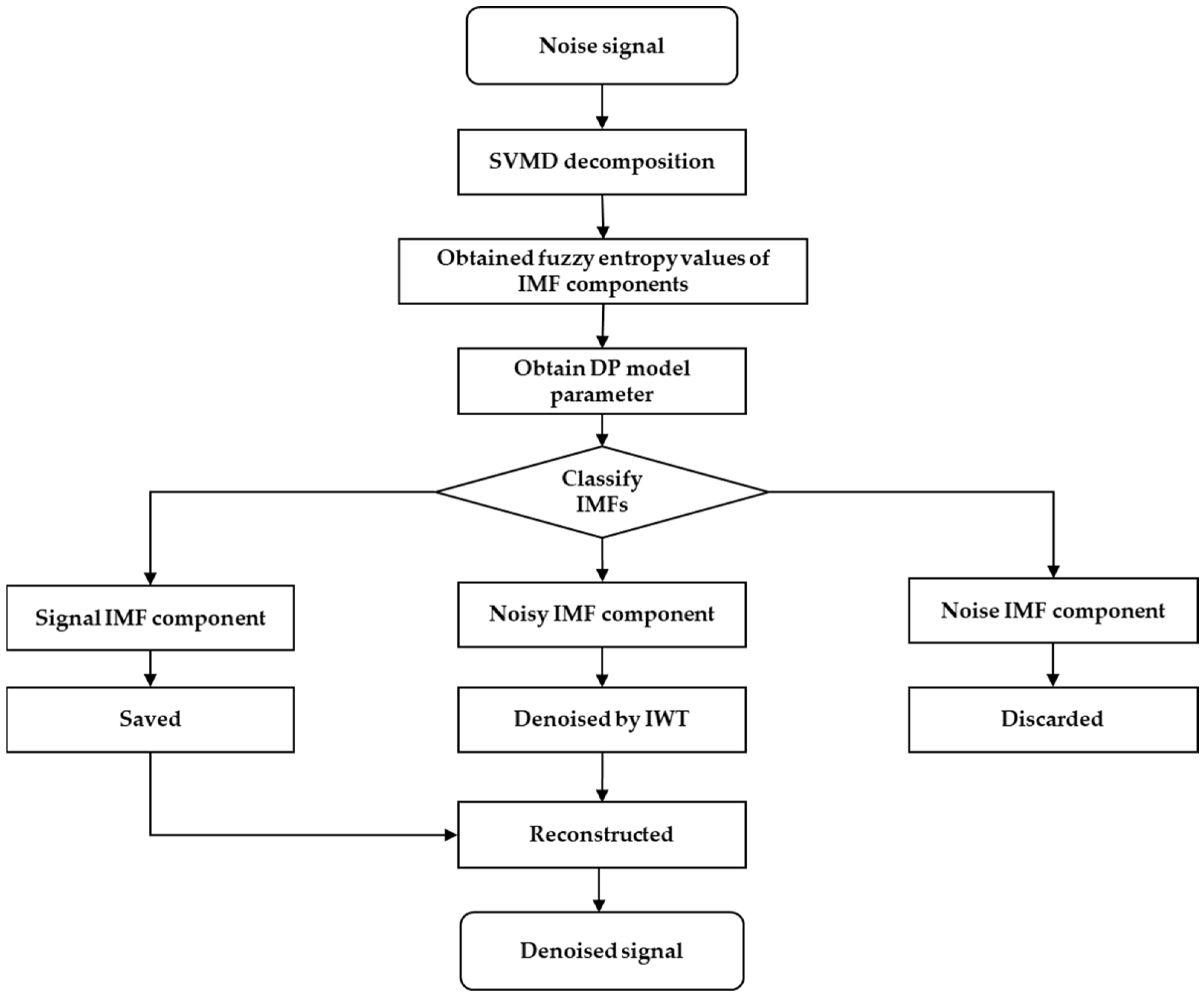
2.5. The SVMD-DP-IWT Method

Building upon the aforementioned concepts, we propose the SVMD-DP-IWT (sqtwolog) method with the sqtwolog threshold and the SVMD-DP-IWT (minimaxi) method with the minimaxi threshold for extracting time–frequency characteristics. To mitigate the impact of noise on signals, we developed the following SVMD-DP-IWT method steps flowchart as shown in Figure 1. First, SVMD decomposes the signal, and the DP model classifies the decomposed components into signal IMFs, noisy IMFs, and noise-dominated IMFs. The noisy IMF components are then denoised using IWT. Finally, the processed IMFs are used to reconstruct the signal, yielding a denoised output. Figure 1 illustrates the workflow of the SVMD-DP-IWT method.

The detailed procedures of the SVMD-DP-IWT method are outlined as follows:

(1) The parameters for initiating SVMD signal decomposition are set, with the penalty factor fixed at 2000, followed by signal decomposition;

(2) The IMF decomposition components are obtained, and the fuzzy entropy values for each component are calculated;

(3) The threshold values are determined using the DP model functions, and the signal IMF, noisy IMF, and noise IMF are identified;

(4) The wavelet basis function selected for decomposition is db4, with the number of decomposition layers set to 3. The noise in the noisy IMF is denoised using the IWT, and the new signal is reconstructed using the signal IMF and the denoising noisy IMF.

2.6. Evaluation Index and Performance Comparison

To accurately evaluate the performance of the SVMD-DP-IWT method, a series of signal processing steps—decomposition, denoising, and reconstruction—are applied to the signal. The signal-to-noise ratio (SNR) is used as an objective metric to assess and compare the effectiveness of noise reduction techniques [21]. This metric quantifies the efficacy of noise attenuation and is mathematically defined by the following equation:

$$\mathrm{SNR}=10\cdot \log {\displaystyle \frac{{\displaystyle \sum _{i=1}^N|}x(i){|}^2}{{\displaystyle \sum _{i=1}^N|}\widehat{x}(i)-x(i){|}^2}}$$

(20)

The root mean square error (RMSE) is a metric for evaluating method performance [22,23]. It is calculated by taking the square root of the mean of the squared differences between predicted and actual values. In the contrived experiment presented in this article, the unperturbed signal, free from noise and outliers, is used as the reference value.

$$\mathrm{RMSE}=\sqrt{{\displaystyle \frac{1}{N}}{\displaystyle \sum _{i=1}^N{\left(\widehat{x}(i)-x(i)\right)}^2}}$$

(21)

Here, $\widehat{x}(i)$ is the signal without noise and $x(i)$ is the signal with processing methods.

Skewness is used to measure the asymmetry of data distribution, and its calculation formula is:

$$\mathrm{Skewness}(x)={\displaystyle \frac{\frac{1}{N}{\displaystyle \sum _{i=1}^N{\left(x(i)-x_0\right)}^3}}{{\left(\frac{1}{N}{\displaystyle \sum _{i=1}^N{\left(x(i)-x_0\right)}^2}\right)}^{\frac{3}{2}}}}$$

(22)

where $x_0$ is the sample mean.

Kurtosis is a statistical term that quantifies the degree of sharpness in a data distribution. Kurtosis is often computed using the following formula:

$$\mathrm{Kurtosis}(x)={\displaystyle \frac{\frac{1}{N}{\displaystyle \sum _{i=1}^N{\left(x(i)-x_0\right)}^4}}{{\left(\frac{1}{N}{\displaystyle \sum _{i=1}^N{\left(x(i)-x_0\right)}^2}\right)}^2}}$$

(23)

A kurtosis value of 3 is a characteristic feature of the normal distribution. If the kurtosis value is greater than 3, it indicates that the data distribution is more peaked than the normal distribution; if the kurtosis value is less than 3, the data distribution is flatter than the normal distribution.

3. Experiment Analysis

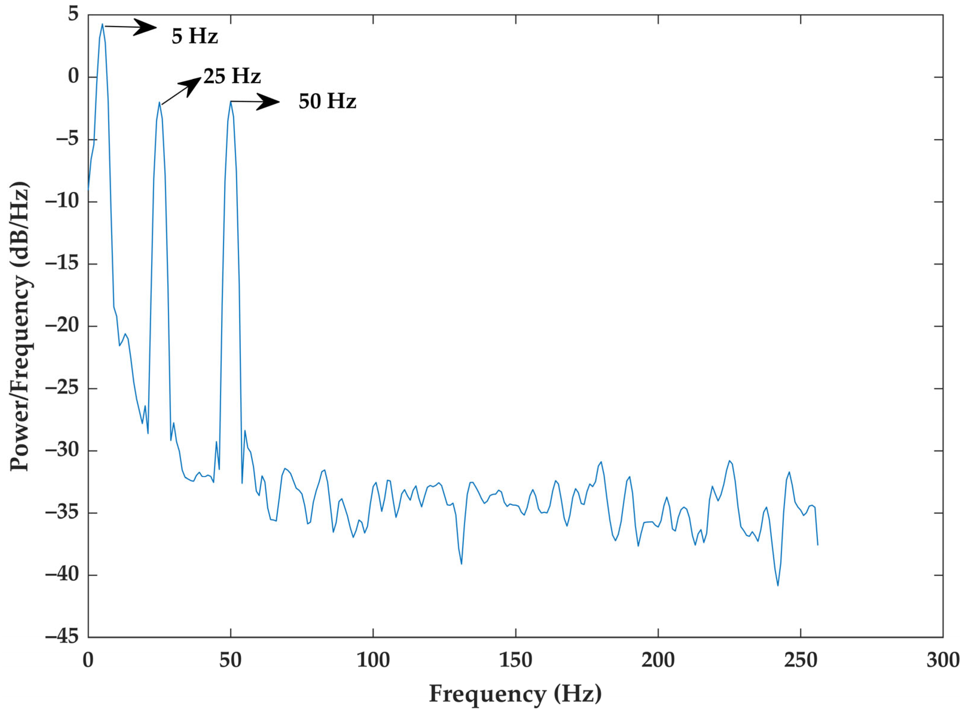
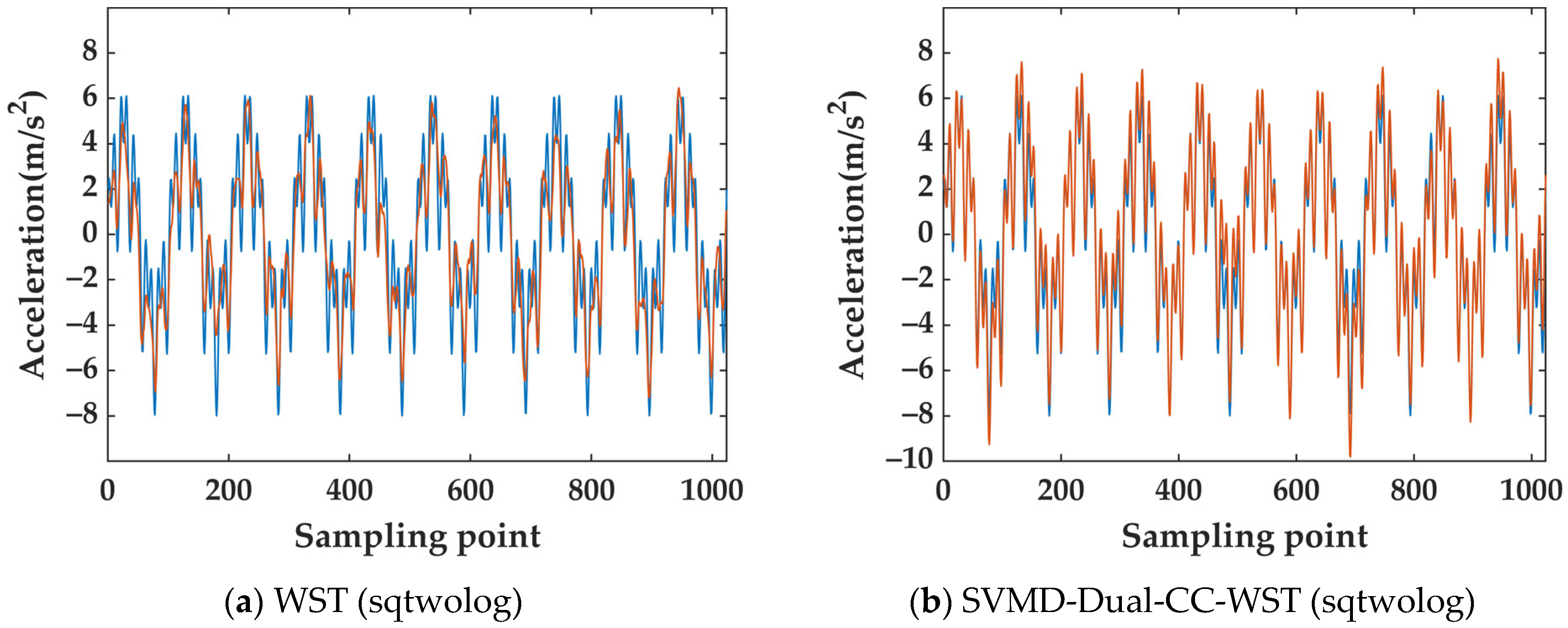
3.1. Simulated Signal

A simulation test was conducted to validate the proposed method. The test signal consisted of two sine waves and one cosine wave, with frequencies of 5 Hz, 25 Hz, and 50 Hz, and amplitudes of 4 m/s², 2 m/s², and 2 m/s², respectively. The clean signal was contaminated by additive noise, which included zero-mean Poisson noise (variance = 0.1) and colored noise. The total sampling duration was 2 s, with a sampling frequency of 512 Hz, resulting in 1024 data points. The simulated signal is generated by Equation (24). While ideal noise follows a Gaussian distribution, actual measurements involve mixed noise; thus, colored noise and Poisson noise were added to the clean signal, which exhibited significant oscillation and shift after the noise addition. Figure 2 illustrates both the clean and noise-contaminated signals.

$$\left\{\begin{array}{c}{x}_1(t)=4\sin (10\pi t)\\ x_2(t)=2\sin (50\pi t)\\ x_3(t)=2\cos (100\pi t)\\ x=x_1(t)+x_2(t)+x_3(t)+v(t)\end{array}\right.$$

(24)

here, $x(t)$ is the clean signal and $v(t)$ is mixed noise. The colored noise is generated by Equation (25)

$$\left\{\begin{array}{c}color\_noise(1)=0.9781\\ color\_noise(i)=0.9781\cdot color\_noise(i-1)+0.342\cdot \mathcal{N}(0,1)\end{array}\right.$$

(25)

where $\mathcal{N}(0,1)$ denotes a standard normal distribution random variable.

The Welch power-spectrum estimation technique improves the accuracy and reliability of spectral analysis. It is used to estimate the power spectrum of the signal, as shown in Figure 3, which reveals signal frequencies at 5 Hz, 25 Hz, and 50 Hz.

Table 2. RMSE and SNR comparison of four signal processing methods (WST (sqtwolog), SVMD-Dual-CC-WST (sqtwolog), SVMD-DP-IWT (sqtwolog), SVMD-DP-IWT (minimaxi)) via 10 simulation experiments.

	WST (Sqtwolog)		SVMD-Dual-CC-WST (Sqtwolog)		SVMD-DP-IWT (Sqtwolog)		SVMD-DP-IWT (Minimaxi)
	RMSE (m/s2)	SNR	RMSE (m/s2)	SNR	RMSE (m/s2)	SNR	RMSE (m/s2)	SNR
1	1.3302	8.3108	0.7076	13.7937	0.5751	15.5941	0.5724	15.6352
2	1.5701	6.8705	0.6577	14.4287	0.6499	14.5321	0.9161	11.5503
3	1.3179	8.3912	0.7452	13.3435	0.6674	14.3014	0.6623	14.3683
4	1.4426	7.6062	0.6928	13.9774	0.6476	14.5633	0.7225	13.6119
5	1.4859	7.3495	0.5759	15.5826	0.6397	14.6688	0.6661	14.3179
6	1.4345	7.6547	0.7867	12.8728	0.7025	13.8561	0.6805	14.1318
7	1.4298	7.6836	0.6336	14.7529	0.7043	13.8344	0.5216	16.4422
8	1.4227	7.7265	0.5793	15.5313	0.8403	12.3005	0.6476	14.5626
9	1.3453	8.2125	0.731	13.5105	0.7251	13.5806	0.7361	13.4501
10	1.3841	7.9658	0.7688	13.0727	0.6279	14.8316	0.6036	15.174

presents the statistical results of the RMSE and SNR metrics for the four methods applied to the signals across 10 simulation experiments.

The simulation experiment was conducted 10 times. According to Table 2, SVMD-Dual-CC-WST (sqtwolog), SVMD-DP-IWT (sqtwolog), and SVMD-DP-IWT (minimaxi) exhibit more stable denoising effects than WST, although some differences remain. Due to space constraints, only one set of experimental results is analyzed and discussed. The denoising results of the four methods are shown in Figure 4, and the displacement results are provided in Figure 5. The average values of SNR and RMSE across the 10 simulation experiments are also presented in

Table 3. RMSE and SNR performance of four denoising methods (WST (sqtwolog), SVMD-Dual-CC-WST (sqtwolog), SVMD-DP-IWT (sqtwolog), SVMD-DP-IWT (minimaxi)) on mixed noise: averaged results from 10 simulations.

Method	RMSE (m/s2)	SNR
WST (sqtwolog)	1.4163	7.7771
SVMD-Dual-CC-WST (sqtwolog)	0.6878	14.0866
SVMD-DP-IWT (sqtwolog)	0.6780	14.2063
SVMD-DP-IWT (minimaxi)	0.6729	14.3244

.

Figure 4 and Figure 5 show that the statistical results of accelerometer errors for the four methods indicate that SVMD-DP-IWT (sqtwolog) achieves the best denoising effect, while WST with the sqtwolog threshold (WST (sqtwolog)) exhibits the largest error. SVMD-Dual-CC-WST and SVMD-DP-IWT (minimaxi) perform second, with SVMD-DP-IWT (sqtwolog) showing the slightest error. Indicating that SVMD-DP-IWT (sqtwolog) and SVMD-DP-IWT (minimaxi) have certain advantages in dealing with mixed noise

As shown in Table 3, SVMD-Dual-CC-WST, SVMD-DP-IWT (sqtwolog), and SVMD-DP-IWT (minimaxi) demonstrate superior performance compared to the conventional WST method. The RMSE improves by 51.44%, 52.13%, and 52.49%, respectively. Furthermore, the signal-to-noise ratio (SNR) shows significant enhancement, increasing from the baseline value of 7.7771 (WST) to 14.0866, 14.2063, and 14.3244 for the three methods, respectively. This indicates substantially better noise suppression capabilities while preserving critical signal features.

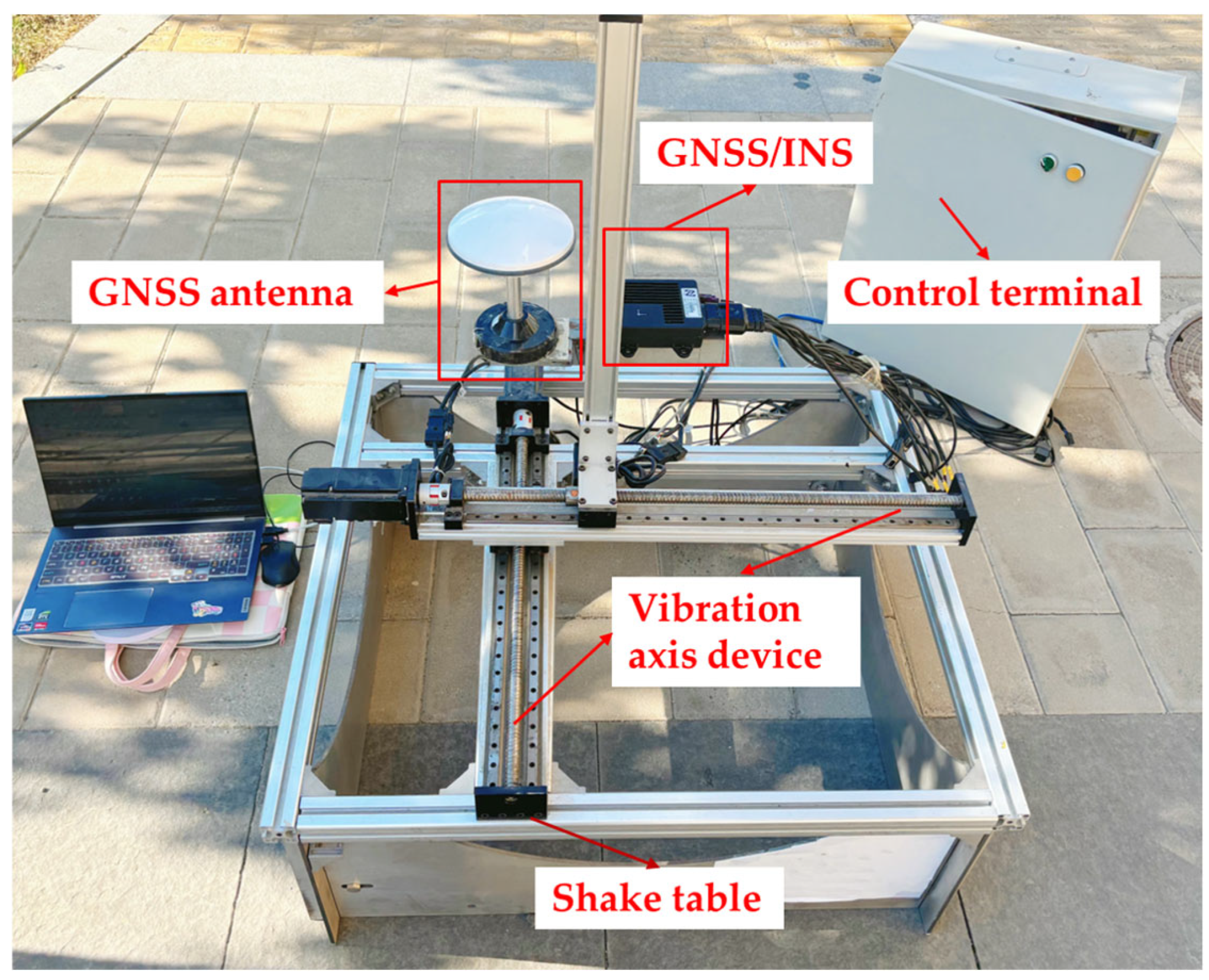
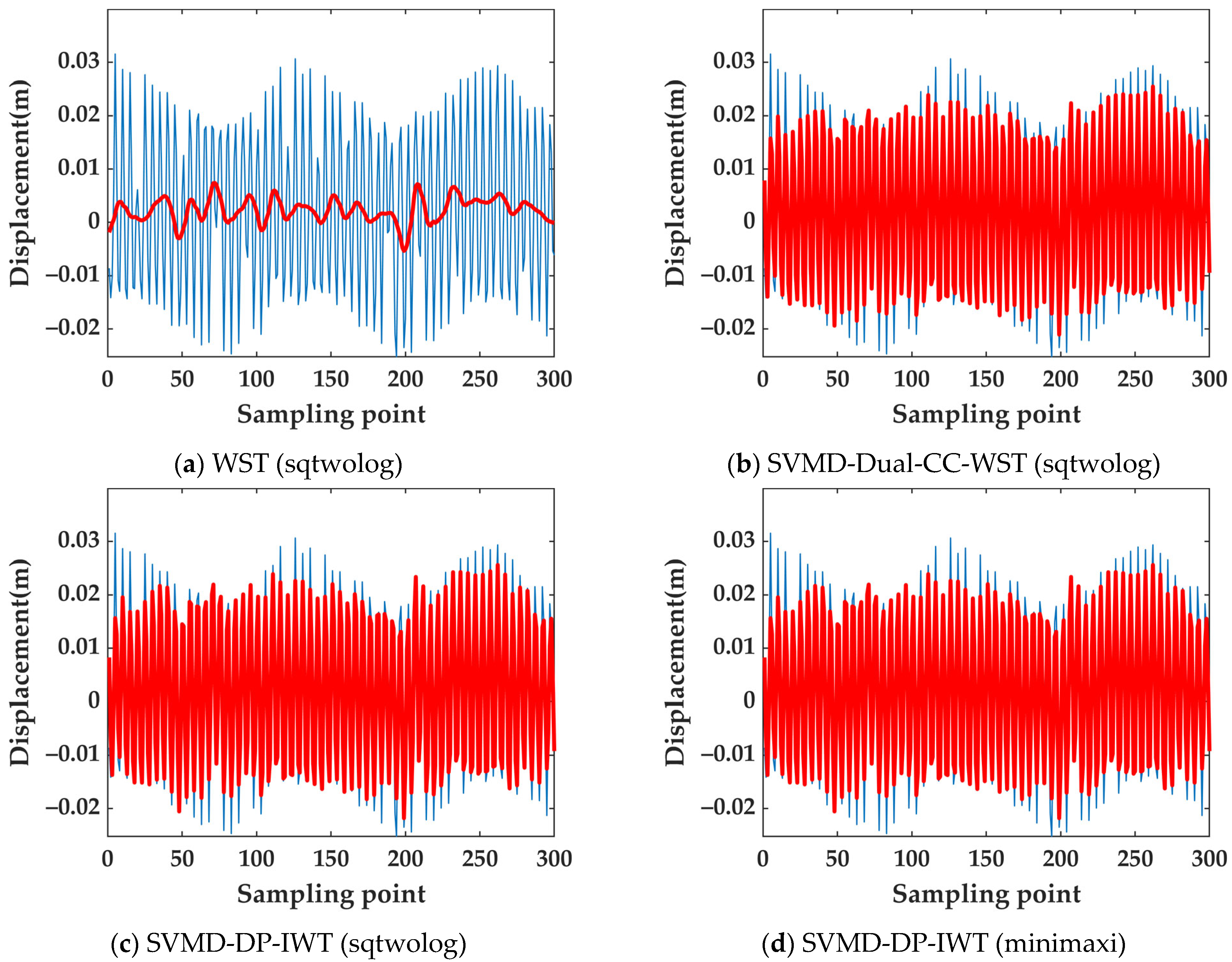
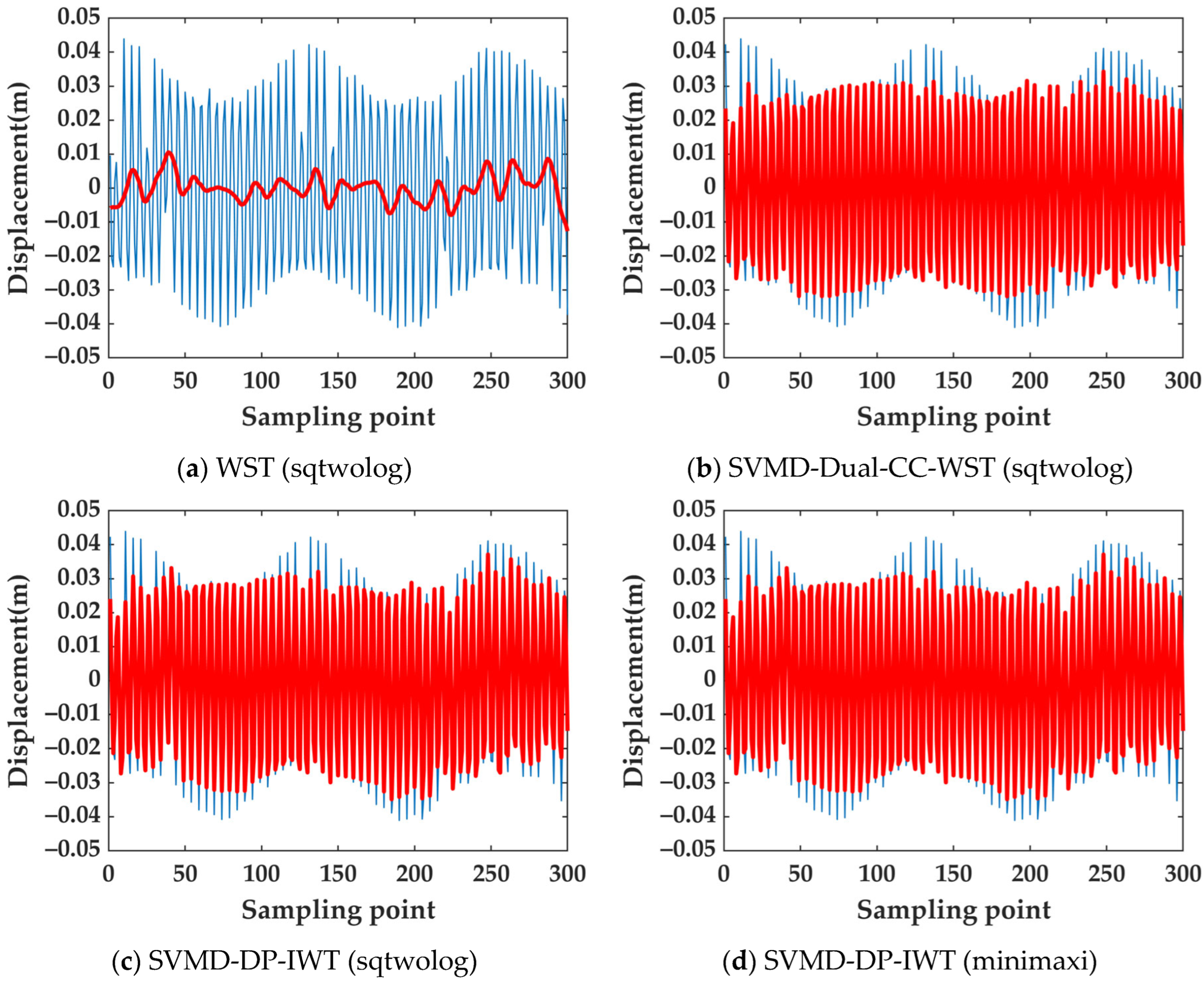
3.2. GNSS Vibration Monitoring Experiment

To verify the reliability of the algorithm, an outdoor GNSS vibration monitoring experiment was designed. The vibration simulation system, as shown in Figure 6, mainly comprises a mobile control system, a data acquisition system (a GNSS/inertial navigation system (INS) device and a GNSS antenna), and a shake table. A GNSS/INS was placed on the vibration table, and a control terminal was used to control the vibration frequency and amplitude of the GNSS/INS device. Real-Time Kinematic positioning (RTK) technology is used to obtain vibration displacement sequences [24,25]. Two GNSS signal vibration tests were conducted with the same frequency (1 Hz) and sampling frequency (5 Hz) but different amplitudes: GNSS Signal 1 at 30 mm and GNSS Signal 2 at 50 mm. As shown in Figure 7 and Figure 8, the maximum amplitude remained within the ranges of 30 mm and 50 mm, with no obvious impact vibrations observed, and the blue line represents the GNSS signal, and the red line represents the denoised signal. Monitoring locations with missing data were obtained through cubic spline interpolation.

Table 4. Key metrics and parameters of GNSS/INS performance.

Parameter	Details
Supported Constellations	BDS: B1/B2; GPS: L1/L2; GLONASS: L1/L2; GALILEO: E1/E5b
Positioning Accuracy	- RTK (RMS): Horizontal 1 cm + 1 ppm, Vertical 1.5 cm + 1 ppm - DGPS: Horizontal 0.5 m, Vertical 1 m
Update Rate	- GNSS: 5 Hz, 10 Hz - Integrated Navigation: 100 Hz, 200 Hz
INS Performance	- Position Hold: 3.75 m (1σ) for 1 km/2 min - Heading Drift: 0.15°/min - Odometer—Fused Position: 2‰

presents the key metrics and parameters of GNSS/INS performance. In terms of positioning accuracy, the root mean square (RMS) error of RTK positioning is 1 cm + 1 ppm (RMS) in the horizontal direction and 1.5 cm + 1 ppm (RMS) in the vertical direction. The accuracy of the differential global positioning system (DGPS) is 0.5 m in the horizontal direction and 1 m in the vertical direction.

Table 5. Statistical analysis of four denoising methods (WST, SVMD-Dual-CC-WST, SVMD-DP-IWT Variants) on two GNSS signals: mean, variance, kurtosis, and skewness evaluation.

	Method	Mean (mm)	Variance (mm2)	Skewness	Kurtosis
GNSS Signal 1	Before denoising	2.2958	0.2061	0.0691	2.0554
	WST (sqtwolog)	2.2951	0.0049	−0.3565	3.5635
	SVMD-Dual-CC-WST (sqtwolog)	2.3071	0.1763	0.0140	1.5714
	SVMD-DP-IWT (sqtwolog)	2.3178	0.1772	0.0141	1.5853
	SVMD-DP-IWT (minimaxi)	2.3178	0.1772	0.0141	1.5853
GNSS Signal 2	Before denoising	−0.0352	0.4966	0.0385	2.0513
	WST (sqtwolog)	−0.0903	0.0156	0.1151	3.2631
	SVMD-Dual-CC-WST (sqtwolog)	−0.0009	0.4349	−0.0001	1.5507
	SVMD-DP-IWT (sqtwolog)	−0.0318	0.4419	0.0005	1.5861
	SVMD-DP-IWT (minimaxi)	−0.0318	0.4419	0.0005	1.5861

presents an analysis of 300 consecutive sampling points using four distinct methods, with statistical evaluation metrics including the mean, variance, skewness, and kurtosis.

Figure 7 and Figure 8 present the processing results of four different methods applied to GNSS Signal 1 and GNSS Signal 2.

As shown in Figure 7, the amplitude remains within 30 mm. The WST method exhibits a smaller amplitude fluctuation range, effectively eliminating the vibration characteristics. Based on Table 5 and Figure 7, in comparison with the WST method, the SVMD-DP-IWT (sqtwolog), SVMD-DP-IWT (minimaxi), and SVMD-Dual-CC WST (sqtwolog) methods extract more features. There are no significant differences in the mean, variance, and skewness among the three methods of SVMD-DP-IWT (sqtwolog), SVMD-DP-IWT (minimaxi), and SVMD-Dual-CC WST (sqtwolog). However, the kurtosis value of the SVMD-Dual-CC WST (sqtwolog) algorithm deviates least from 3, indicating that most of its data are closely distributed around the mean with a smaller fluctuation range. The kurtosis values of SVMD-DP-IWT (sqtwolog) and SVMD-DP-IWT (minimaxi) are slightly larger than those of SVMD-Dual-CC WST (sqtwolog), suggesting that their fluctuation ranges are greater.

As can be seen from Figure 8, the amplitude remains within 50 mm. Similarly, the WST method shows a smaller amplitude fluctuation range, suppressing most of the vibration characteristics. Based on Table 5 and Figure 8, compared with the WST method, the SVMD-DP-IWT (sqtwolog), SVMD-DP-IWT (minimaxi), and SVMD-Dual-CC WST (sqtwolog) methods extract more features. There are no significant differences in the mean and variance among the three methods of SVMD-DP-IWT (sqtwolog), SVMD-DP-IWT (minimaxi), and SVMD-Dual-CC WST (sqtwolog). However, the skewness of the SVMD-Dual-CC WST (sqtwolog) algorithm is close to 0, and its kurtosis value deviates least from 3, indicating that most of its data are closely distributed around the mean with a smaller fluctuation range. The skewness values of SVMD-DP-IWT (sqtwolog) and SVMD-DP-IWT (minimaxi) are positive, consistent with the skewness direction of the pre-denoising signal, showing right-skewed distribution characteristics. Their kurtosis values are slightly larger than those of SVMD-Dual-CC WST (sqtwolog), indicating larger fluctuation ranges.

When Figure 7 and Figure 8 are compared, it is found that the three methods, SVMD-DP-IWT (sqtwolog), SVMD-DP-IWT (minimaxi), and SVMD-Dual-CC WST (sqtwolog), can all effectively extract vibration features. Under the same conditions, compared with GNSS Signal 1 (amplitude: 30 mm), GNSS Signal 2 for extracting vibration features is more prominent in terms of skewness and kurtosis. However, due to the limitations of experimental conditions (relatively low GNSS vibration and sampling frequencies), the methods are unable to detect high-frequency vibrations [26]. On this basis, an accelerometer vibration monitoring experiment is designed.

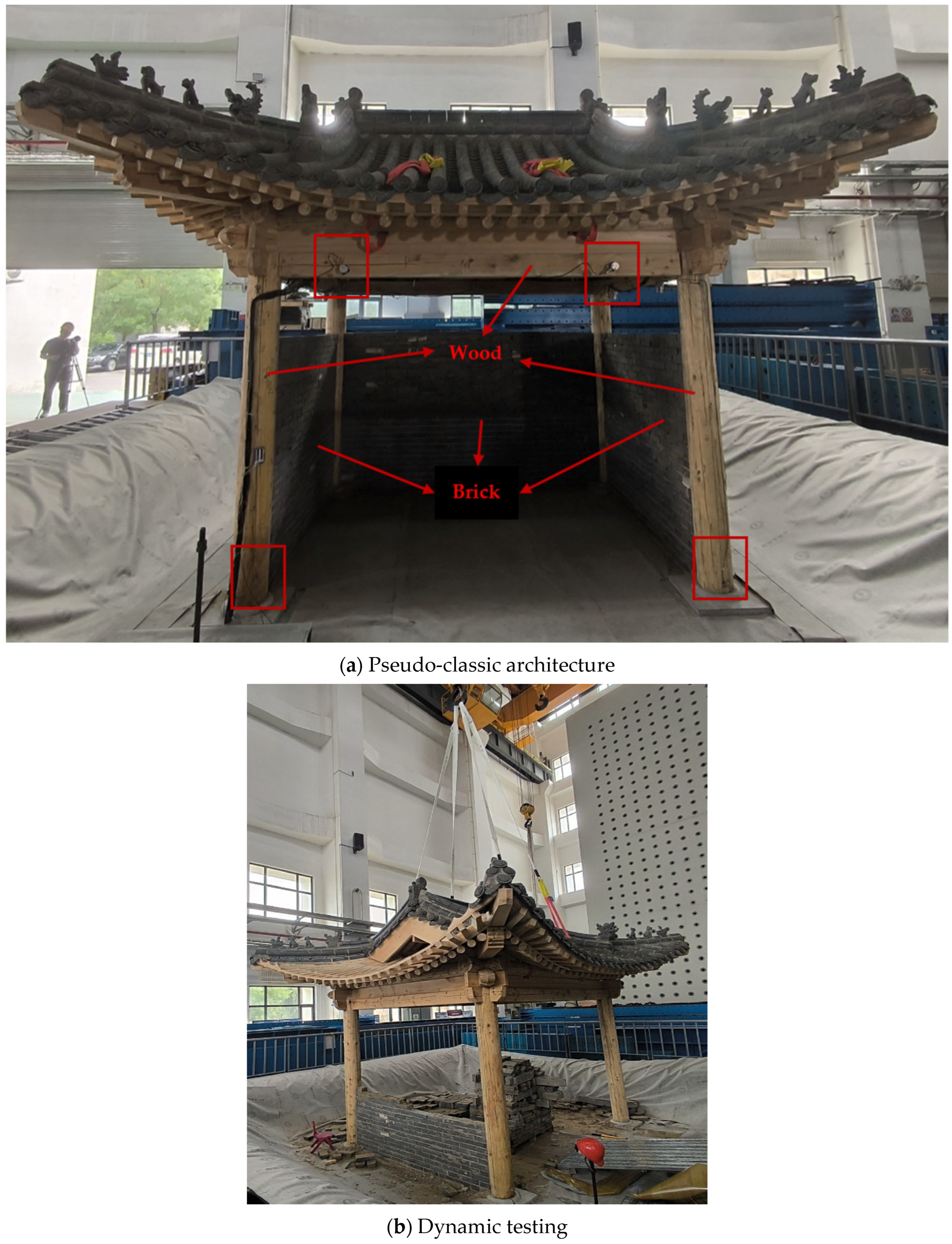
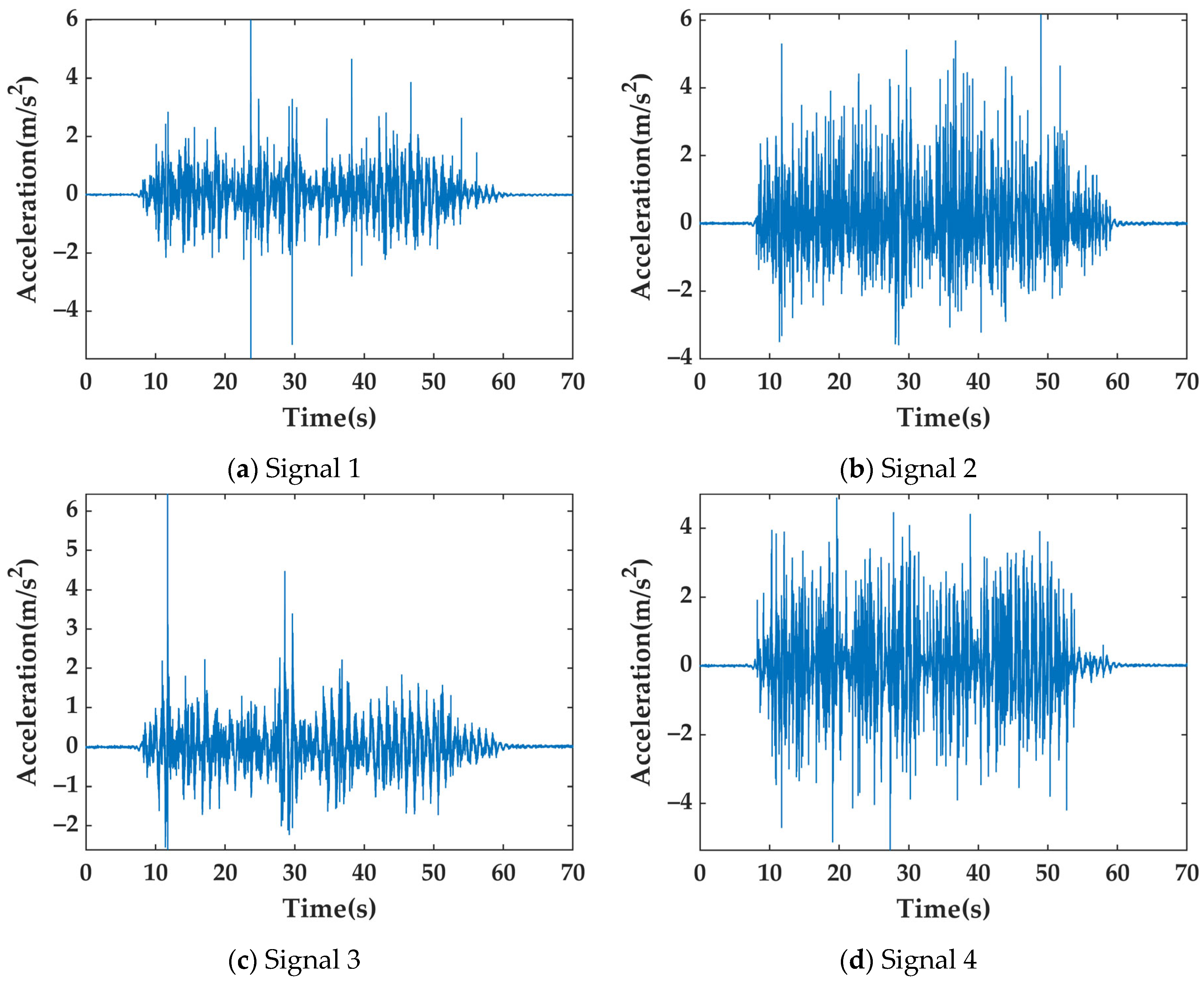
3.3. Engineering Measurement Analysis

Experiments were conducted using the large-scale multi-functional shaking table at the Beijing University of Civil Engineering and Architecture. This facility is capable of accurately simulating seismic wave inputs with varying amplitudes and frequencies, enabling a comprehensive evaluation of the dynamic response of ancient-style building structures to earthquake ground motions. The experimental subject was a typical model of pseudo-classic architecture, featuring a hybrid timber-masonry structure with a single-eave hip-and-gable roof. The main structural framework was constructed with wooden components joined by mortise-and-tenon joints, complemented by brick walls built in three orthogonal directions as auxiliary supports. The building’s planar column grid measured 3.85 m in length and 3.12 m in width, with a total structural height of approximately 4.20 m. For sensor deployment, the research team strategically placed 32 accelerometers at key structural locations, with the experimental setup and sensor installation points shown in Figure 9 and Figure 10. In Figure 10, each red dot marker represents a sensor configured to simultaneously collect acceleration or rope displacement data in both the X- and Y-axes. The red-boxed areas in Figure 9 correspond to installation points for specialized monitoring equipment, designed to provide detailed monitoring of localized structural responses. The blue box in Figure 10a indicates the accelerometer’s installation position for signal source analysis in this study.

The experimental loading conditions are designed to replicate the behavior of the model structure under the 8-degree earthquake intensity on the rare earthquake scale. The seismic effects are simulated under bidirectional seismic motion in both the X- and Y-axes.

Table 6. Main oscillator accelerations in X and Y directions under 8-degree earthquake intensity on the rare earthquake excitation.

	Main Oscillator Y Direction (m/s2)	Main Oscillator X Direction (m/s2)
8-degree earthquake intensity	4	3.4

presents the experimental vibration protocol. The main oscillator’s acceleration is 4 m/s² in the Y-direction and 3.4 m/s² in the X-direction.

Figure 10a displays the instrument layout, highlighting accelerometers 11, 13, 15, and 17. Figure 10b illustrates their installation near the horizontal beams of the pavilion’s four columns. Data were acquired at 200 Hz using LC0701-5 accelerometers, with key parameters provided in

Table 7. Key metrics and parameters of accelerometer performance.

Main Technical Indicators	Parameters
Sensitivity	300 mV/g
Range	±5 g
Resolving power	0.05 g
Frequency response range	DC-2500 Hz (−3 dB)
Weight	35 gm

.

Figure 11 presents a comparative analysis of the vibration response characteristics recorded by accelerometers at different locations of the pseudo-classic architecture under rare earthquake conditions. The data were acquired at a sampling rate of 200 Hz over a duration of 71.10 s, resulting in 14,222 valid sampling points, with time (s) on the horizontal axis and amplitude (m/s²) on the vertical axis.

Analysis of the acceleration variations shown in Figure 11 reveals that during both the initial and final phases of the vibration experiment (at sampling intervals of approximately 0 s and 71 s), the acceleration values approached zero. This indicates that the accelerometers remained relatively stable before and after the vibration event. Between 10 s and 60 s of the sampling interval, the acceleration readings exhibited high-frequency oscillations, confirming the occurrence of seismic vibrations during this period. Figure 11a displays a notable fluctuation amplitude, with a positive peak of approximately 6 m/s² and a negative peak of around −5.6 m/s². The high frequency of fluctuations and numerous peaks suggest significant instantaneous acceleration variations, leading to a dispersed energy distribution throughout the vibration process. In Figure 11b, the positive peak reaches 6 m/s², while the negative peak approximates −3.6 m/s². Although the overall fluctuation range resembles that of the first plot, the waveform demonstrates denser oscillations in regions such as sampling points 20 s to 40 s, indicating more concentrated rapid acceleration changes. Figure 11c exhibits a positive peak of roughly 6.4 m/s² and a negative peak of −2.6 m/s², with fewer fluctuation peaks compared to the first two figures. Notably, between 40 s and 60 s, the intensity of acceleration fluctuations diminishes slightly, accompanied by a reduction in energy concentration. Figure 11d shows a positive peak of 5 m/s² and a negative peak of approximately −5.3 m/s². The fluctuation amplitude is smaller than that of the first three plots, and the waveform is comparatively smoother, indicating attenuated instantaneous acceleration changes and more stable energy release during the vibration process. To validate the denoising performance of the proposed SVMD-DP-IWT method under seismic conditions, comparative analyses were conducted with the WST and SVMD-Dual-CC-WST methods.

Table 8. Statistical analysis of four denoising methods (WST, SVMD-Dual-CC-WST, SVMD-DP-IWT Variants) on four accelerometer signals: mean, variance, kurtosis, and skewness evaluation.

	Method	Mean (m/s2)	Variance (m2/s4)	Skewness	Kurtosis
Signal 1	Before denoising	0.0232	0.4341	−0.2005	3.5368
	WST (sqtwolog)	0.0233	0.2241	−0.3486	3.0688
	SVMD-Dual-CC-WST (sqtwolog)	0.0204	0.2219	−0.1984	2.7202
	SVMD-DP-IWT (sqtwolog)	0.0205	0.2221	−0.1991	2.7246
	SVMD-DP-IWT (minimaxi)	0.0205	0.2221	−0.1991	2.7246
Signal 2	Before denoising	0.0285	0.6442	0.2516	6.2358
	WST (sqtwolog)	0.0287	0.2564	−0.2438	4.2555
	SVMD-Dual-CC-WST (sqtwolog)	0.0241	0.2248	−0.2955	4.0302
	SVMD-DP-IWT (sqtwolog)	0.0247	0.2602	−0.1103	4.2131
	SVMD-DP-IWT (minimaxi)	0.0247	0.2602	−0.1103	4.2132
Signal 3	Before denoising	0.0015	0.4380	0.8008	13.5810
	WST (sqtwolog)	0.0017	0.2842	−0.5408	4.5606
	SVMD-Dual-CC-WST (sqtwolog)	0.0014	0.2664	−0.5135	4.3759
	SVMD-DP-IWT (sqtwolog)	0.0015	0.2680	−0.5138	4.4176
	SVMD-DP-IWT (minimaxi)	0.0015	0.2749	−0.3765	4.6807
Signal 4	Before denoising	0.0007	0.9585	−0.0722	5.1131
	WST (sqtwolog)	0.0011	0.2786	−0.0491	2.4973
	SVMD-Dual-CC-WST (sqtwolog)	0.0008	0.2459	−0.1795	2.2451
	SVMD-DP-IWT (sqtwolog)	0.0007	0.6101	0.0747	3.3963
	SVMD-DP-IWT (minimaxi)	0.0007	0.6101	0.0747	3.3963

presents an analysis of 2001 to 3000 consecutive sampling points using four distinct methods, with statistical evaluation metrics including the mean, variance, skewness, and kurtosis.

Figure 12, Figure 13, Figure 14 and Figure 15 present the processing results of four types of signals using four different methods.

From Figure 12, it can be observed that Signal 1 exhibits a narrower vibration amplitude range in the accelerometer readings compared to the other three signals, indicating relatively milder shock vibrations at this location. The SVMD-DP-IWT (sqtwolog), SVMD-DP-IWT (minimaxi), and SVMD-Dual-CC-WST (sqtwolog) methods extract more features than the WST method. As shown in Figure 12, while WST (sqtwolog) significantly attenuates these features, the other three methods—SVMD-Dual-CC-WST (sqtwolog), SVMD-DP-IWT (sqtwolog), and SVMD-DP-IWT (minimaxi)—better preserve the shock vibration characteristics. Post-denoising analysis shows that these three methods result in substantially lower values for mean, variance, and skewness compared to WST. Additionally, their kurtosis values deviate from the baseline value of 3 (indicative of a normal distribution), displaying flatter data distribution profiles.

From Figure 13, it can be observed that SVMD-DP-IWT (sqtwolog) extracts features more clearly compared to WST (sqtwolog) and SVMD-Dual-CC-WST (sqtwolog). Based on the vibration amplitude, it is evident that the amplitude of Signal 2 is larger than that of Signal 1. Therefore, when the amplitude is larger, SVMD-DP-IWT (sqtwolog) and SVMD-DP-IWT (minimaxi) are more effective at extracting vibration features compared to the other two methods. Signal 2 exhibits negative skewness values, indicating a left-skewed distribution. The skewness values of SVMD-DP-IWT (sqtwolog) and SVMD-DP-IWT (minimaxi) are closer to zero, suggesting a more symmetric distribution with reduced left-right asymmetry. Additionally, the mean and variance values of these two methods are higher than those of the other methods, further confirming their better preservation of shock vibration characteristics. In the 300 to 400 sampling point range in Figure 13, distinct differences can be observed when comparing SVMD-Dual-CC-WST and WST. Specifically, the SVMD-Dual-CC-WST curve appears smoother, indicating stronger noise suppression. In contrast, the SVMD-DP-IWT (sqtwolog) and SVMD-DP-IWT (minimaxi) methods retain more of the shock-induced vibration features, as evidenced by the higher amplitude fluctuations in this interval.

As shown in Figure 14, for Signal 3, the skewness values are all negative, indicating a left-skewed distribution. Compared to the WST (sqtwolog), SVMD-Dual-CC-WST (sqtwolog), and SVMD-DP-IWT (sqtwolog) methods, the skewness value of the SVMD-DP-IWT (minimaxi) method is closer to zero, suggesting a relatively smaller left skew and a more symmetric distribution. Additionally, the differences in mean and variance between the SVMD-DP-IWT (minimaxi) and other methods are relatively small, indicating that its performance in handling signal stability is comparable to the other three methods. Regarding kurtosis, all methods show a decrease in kurtosis values, indicating effective noise removal. However, the SVMD-DP-IWT (minimaxi) method still has the highest kurtosis value among the four methods, indicating that it preserves more of the shock vibration characteristics during the denoising process. In particular, within the 300 to 400 sampling point range in Figure 14, SVMD-DP-IWT (minimaxi) retains more prominent vibration features, further confirming its advantage in preserving shock vibration characteristics. Compared to SVMD-DP-IWT (sqtwolog), the SVMD-DP-IWT (minimaxi) method demonstrates superior information retention under the same conditions, better reflecting the shock vibration characteristics in the signal. Therefore, in terms of signal feature extraction, the SVMD-DP-IWT (minimaxi) method exhibits superior performance in this signal.

From Figure 15, it is clearly observed that compared to SVMD-Dual-CC-WST, the vibration characteristics of WST (sqtwolog) are more prominent. The SVMD-Dual-CC-WST (sqtwolog) method effectively removes more vibration characteristics as noise, resulting in smoother curves. On the other hand, SVMD-DP-IWT (sqtwolog) and SVMD-DP-IWT (minimaxi) retain a large amount of information, and the vibration features are clearly visible. However, the downside of these methods is that they cannot effectively quantify the noise content within the information. For Signal 4, the SVMD-DP-IWT (sqtwolog) and SVMD-DP-IWT (minimaxi) methods produce the lowest mean values, the highest variance values, and positive skewness, indicating a more pronounced right-skewed distribution. Their kurtosis values are closer to 3, suggesting that after denoising, the signals approximate a normal distribution. As shown in Figure 15, these two methods retain more shock vibration characteristics, while WST preserves only partial vibration features, and SVMD-Dual-CC-WST retains the least, as observed in the sampling range from 400 to 500.

From Table 8 and Figure 12, Figure 13, Figure 14 and Figure 15, Signal 1 exhibits a left-skewed distribution with a negative skewness value, while Signals 2 and 3 show right-skewed distributions with positive skewness values. Before denoising, the amplitude ranges of the accelerometer measurements for Signals 2 and 3 are [−4, 6] and [−3, 7], respectively, indicating more severe seismic impacts and more frequent state changes compared to Signals 1 and 4. This is reflected in their mean, variance, kurtosis, and skewness values, suggesting that these two positions experience stronger impact vibrations. Regarding the change in index values after denoising, in terms of the mean, all methods except WST (SVMD-Dual-CC-WST, SVMD-DP-IWT (sqtwolog), SVMD-DP-IWT (minimaxi)) result in reduced mean values. For variance, all methods lead to decreases, with SVMD-Dual-CC-WST showing the most significant reduction. In terms of skewness, SVMD-DP-IWT (minimaxi) has an absolute value close to 0. The kurtosis values generally exhibit a downward trend. Except for the WST, the other methods show minimal changes in skewness and greater deviations from 3 in kurtosis, indicating that they retain certain impact vibration features. When comparing the retention of impact vibration features among different denoising methods, SVMD-DP-IWT (sqtwolog) and SVMD-DP-IWT (minimaxi) have higher kurtosis values than SVMD-Dual-CC-WST, suggesting better retention of impact vibration characteristics. Although the WST has a higher kurtosis value than SVMD-DP-IWT (sqtwolog) and SVMD-DP-IWT (minimaxi), it also has larger mean and variance values. The signals processed by SVMD-DP-IWT (sqtwolog) and SVMD-DP-IWT (minimaxi) are more stable than those processed by the WST.

In summary, while SVMD-DP-IWT (sqtwolog) and SVMD-DP-IWT (minimaxi) effectively preserve shock vibration characteristics, they also include more noise, making them less effective in noise quantification. Conversely, the SVMD-Dual-CC-WST and WST methods offer better noise suppression but at the cost of losing significant vibration features.

4. Conclusions

This article proposes a novel denoising method integrating SVMD with fuzzy entropy evaluation criteria. The key conclusions drawn from the analysis are as follows:

(1) Improvement of the Dual-CC thresholding criterion: This study enhances the Dual-CC thresholding criterion by introducing fuzzy entropy as a parameter within the DP model. It combines SVMD and IWT denoising theories to propose the SVMD-DP-IWT model. This integration aims to optimize parameter selection and improve the adaptability of the denoising process for complex vibration signals.

(2) Simulation Results: The proposed method demonstrates significant advantages in processing acceleration signals contaminated with mixed noise. Compared to traditional algorithms, it achieves higher SNR improvements and more accurate retention of impact vibration features, confirming its effectiveness in noisy environments.

(3) GNSS vibration monitoring and engineering measurement for accelerometer results: compared with the SVMD-Dual-CC-WST (sqtwolog) and WST (sqtwolog), the SVMD-DP-IWT method effectively retains key impact vibration signals during denoising. When high-frequency vibrations and obvious impact characteristics are present, the effect becomes better. This feature provides distinct advantages in describing the seismic vibration responses of ancient buildings.

While the study primarily focuses on vibration monitoring experiments of pseudo-classic architecture under simulated strong seismic conditions, some aspects warrant further investigation. Specifically, during the experimental simulation, GNSS and acceleration data were not fully fused for analysis, and rope displacement sensor data were not completely integrated with accelerometer data. To better characterize structural deformation and vibration coupling, a comprehensive multi-sensor fusion approach is needed. Additionally, incorporating deep learning with SVMD for deformation predictive analysis, leveraging neural networks, can enhance the accuracy of vibration trend forecasting.

References

1. Information, V.F.A.; Uva, G.; Information, V.F.A.; Simeone, V.; Information, V.F.A.; Nettis, A.; Information, V.F.A.; Morga, M.; Information, V.F.A.; Doglioni, A. Probabilistic-based assessment of subsidence phenomena on the existing built heritage by combining MTInSAR data and UAV photogrammetry. Struct. Infrastruct. Eng. 2024, 1–16. [Google Scholar] [CrossRef]
2. Wen, G.R.; Zhao, L.; Liu, Z.C.; Wang, J.Y.; Huang, X.B.; Yuan, P. Research on loose bolt localization technology for transmission towers. Struct. Health Monit. 2024, 23, 3134–3155. [Google Scholar] [CrossRef]
3. Jing, C.; Huang, G.; Zhang, Q.; Li, X.; Bai, Z.; Du, Y. GNSS/accelerometer adaptive coupled landslide deformation monitoring technology. Remote Sens. 2022, 14, 3537. [Google Scholar] [CrossRef]
4. Wei, L.; Siyuan, C.; Yangkang, C. Applications of variational mode decomposition in seismic time-frequency analysis. Geophysics 2016, 81, 365–378. [Google Scholar]
5. Dong, L.L.; Xu, N.W.; Zhang, P.; Li, B.; Xiao, P.W.; Sun, Y.P. An ICEEMDAN-WPD based denoising method for MS signals and its engineering application. Nondestruct. Test. Eval. 2025, 40, 1946–1968. [Google Scholar] [CrossRef]
6. Dragomiretskiy, K.; Zosso, D. Variational Mode Decomposition. IEEE Trans. Signal Process. 2014, 62, 531–544. [Google Scholar] [CrossRef]
7. Gu, J.; Peng, Y.X.; Lu, H.; Chang, X.D.; Chen, G.A. A novel fault diagnosis method of rotating machinery via VMD, CWT and improved CNN. Measurement 2022, 200, 111635. [Google Scholar] [CrossRef]
8. Nazari, M.; Sakhaei, S.M. Successive variational mode decomposition. Signal Process. 2020, 174, 107610. [Google Scholar] [CrossRef]
9. Li, Y.X.; Xiao, L.Q.; Tang, B.Z.; Liang, L.L.; Lou, Y.L.; Guo, X.Y.; Xue, X.H. A Denoising Method for Ship-Radiated Noise Based on Optimized Variational Mode Decomposition with Snake Optimization and Dual-Threshold Criteria of Correlation Coefficient. Math. Probl. Eng. 2022, 2022, 8024753. [Google Scholar] [CrossRef]
10. Jauhari, K.; Rahman, A.Z.; Al Huda, M.; Azka, M.; Widodo, A.; Prahasto, T. A feature extraction method for intelligent chatter detection in the milling process. J. Intell. Manuf. 2024. [Google Scholar] [CrossRef]
11. Zhou, X.Y.; Li, Y.B.; Jiang, L.; Zhou, L. Fault feature extraction for rolling bearings based on parameter-adaptive variational mode decomposition and multi-point optimal minimum entropy deconvolution. Measurement 2021, 173, 108469. [Google Scholar] [CrossRef]
12. Peng, D.F.; Li, H.K.; Ou, J.Y.; Wang, Z.D. Milling chatter identification by optimized variational mode decomposition and fuzzy entropy. Int. J. Adv. Manuf. Tech. 2022, 121, 6111–6124. [Google Scholar] [CrossRef]
13. Xu, C.J.; Yang, J.T.; Zhang, T.Y.; Li, K.; Zhang, K. Adaptive parameter selection variational mode decomposition based on a novel hybrid entropy and its applications in locomotive bearing diagnosis. Measurement 2023, 217, 113110. [Google Scholar] [CrossRef]
14. Ma, H.M.; Xu, Y.F.; Wang, J.Y.; Song, M.M.; Zhang, S.L. SVMD coupled with dual-threshold criteria of correlation coefficient: A self-adaptive denoising method for ship-radiated noise signal. Ocean Eng. 2023, 281, 114931. [Google Scholar] [CrossRef]
15. Xue, H.; Chen, J.T.; Bai, Y.L.; Ye, C.L. Train axlebox bearing composite fault denoising method based on SVMD and dual threshold classification criteria. Meas. Sci. Technol. 2025, 36, 026139. [Google Scholar] [CrossRef]
16. Gao, S.Z.; Li, T.C.; Zhang, Y.M.; Pei, Z.M. Fault diagnosis method of rolling bearings based on adaptive modified CEEMD and 1DCNN model. ISA Trans. 2023, 140, 309–330. [Google Scholar] [CrossRef]
17. Li, Y.X.; Zhang, C.L.; Zhou, Y.H. A Novel Denoising Method for Ship-Radiated Noise. J. Mar. Sci. Eng. 2023, 11, 1730. [Google Scholar] [CrossRef]
18. Chen, W.; Wang, Z.; Xie, H.; Yu, W. Characterization of Surface EMG Signal Based on Fuzzy Entropy. IEEE Trans. Neural Syst. Rehabil. Eng. 2007, 15, 266–272. [Google Scholar] [CrossRef] [PubMed]
19. Donoho, D.L. De-noising by soft-thresholding. IEEE Trans. Inf. Theory 1995, 41, 613–627. [Google Scholar] [CrossRef]
20. Tang, P.; Guo, B.P. Wavelet denoising based on modified threshold function optimization method. J. Signal Process. 2017, 33, 102–110. [Google Scholar]
21. Xu, L.; Su, H.Z.; Cai, D.; Zhou, R.L. RDTS Noise Reduction Method Based on ICEEMDAN-FE-WSTD. IEEE Sens. J. 2022, 22, 17854–17863. [Google Scholar] [CrossRef]
22. Mi, X.W.; Liu, H.; Li, Y.F. Wind speed prediction model using singular spectrum analysis, empirical mode decomposition and convolutional support vector machine. Energy Convers. Manag. 2019, 180, 196–205. [Google Scholar] [CrossRef]
23. Zhang, F.Q.; Guo, J.; Yuan, F.; Shi, Y.J.; Li, Z.Y. Research on Denoising Method for Hydroelectric Unit Vibration Signal Based on ICEEMDAN-PE-SVD. Sensors 2023, 23, 6368. [Google Scholar] [CrossRef] [PubMed]
24. Huang, G.W.; Du, S.; Wang, D. GNSS techniques for real-time monitoring of landslides: A review. Satell. Navig. 2023, 4, 5. [Google Scholar] [CrossRef]
25. Wang, D.; Huang, G.W.; Du, Y.; Zhang, Q.; Bai, Z.W.; Tian, J. Stability analysis of reference station and compensation for monitoring stations in GNSS landslide monitoring. Satell. Navig. 2023, 4, 29. [Google Scholar] [CrossRef]
26. El-Sheimy, N.; Youssef, A. Inertial sensors technologies for navigation applications: State of the art and future trends. Satell. Navig. 2020, 1, 2. [Google Scholar] [CrossRef]
Figure 1. The flowchart of the SVMD-DP-IWT method steps.
Remotesensing 17 02057 g001
Figure 2. Composite fault signal: (a) clean signal, (b) add noise signal.
Remotesensing 17 02057 g002
Figure 3. The power spectral density of the add noise signal using Welch’s power-spectrum estimation technique.
Remotesensing 17 02057 g003
Figure 4. Denoising effectiveness of four methods (WST (sqtwolog), SVMD-Dual-CC-WST (sqtwolog), SVMD-DP-IWT (sqtwolog), SVMD-DP-IWT (minimaxi)): a single-simulation evaluation; the red line represents the denoised signal, while the blue line represents the add noise signal.
Remotesensing 17 02057 g004aRemotesensing 17 02057 g004b
Figure 5. The difference between the add noise and denoised signals for four methods (WST (sqtwolog), SVMD-Dual-CC-WST (sqtwolog), SVMD-DP-IWT (sqtwolog), SVMD-DP-IWT (minimaxi)): a single-simulation evaluation.
Remotesensing 17 02057 g005
Figure 6. GNSS vibration monitoring experiment and multiple equipment.
Remotesensing 17 02057 g006
Figure 7. Denoising performance analysis of four methods (WST, SVMD-Dual-CC-WST, SVMD-DP-IWT-sqtwolog, SVMD-DP-IWT-minimaxi) for GNSS Signal 1; the blue line denotes the GNSS signal, and the red line represents the denoised results of each method.
Remotesensing 17 02057 g007
Figure 8. Denoising performance analysis of four methods (WST, SVMD-Dual-CC-WST, SVMD-DP-IWT-sqtwolog, SVMD-DP-IWT-minimaxi) for GNSS Signal 2; the blue line denotes the GNSS signal, and the red line represents the denoised results of each method.
Remotesensing 17 02057 g008
Figure 9. Dynamic testing of pseudo-classic architecture: (a) pseudo-classic architecture, (b) dynamic testing.
Remotesensing 17 02057 g009
Figure 10. Schematic and detailed view of accelerometer layout in the experiment: (a) accelerometer installation schematic diagram; the blue frames represent the installation positions of accelerometers arranged for experimental analysis, (b) accelerometer installation detail diagram.
Remotesensing 17 02057 g010
Figure 11. Comparative analysis of four accelerometer signals under 8-degree earthquake intensity on the rare earthquake excitation.
Remotesensing 17 02057 g011
Figure 12. Denoising performance analysis of four methods (WST, SVMD-Dual-CC-WST, SVMD-DP-IWT-sqtwolog, and SVMD-DP-IWT-minimaxi) for accelerometer Signal 1.
Remotesensing 17 02057 g012
Figure 13. Denoising performance analysis of four methods (WST, SVMD-Dual-CC-WST, SVMD-DP-IWT-sqtwolog, SVMD-DP-IWT-minimaxi) for accelerometer Signal 2.
Remotesensing 17 02057 g013
Figure 14. Denoising performance analysis of four methods (WST, SVMD-Dual-CC-WST, SVMD-DP-IWT-sqtwolog, SVMD-DP-IWT-minimaxi) for accelerometer Signal 3.
Remotesensing 17 02057 g014
Figure 15. Denoising performance analysis of four methods (WST, SVMD-Dual-CC-WST, SVMD-DP-IWT-sqtwolog, SVMD-DP-IWT-minimaxi) for accelerometer Signal 4.
Remotesensing 17 02057 g015