Applications of InSAR for Monitoring Post-Wildfire Ground Surface Displacements

Abstract

Wildfires pose a significant threat to the natural and built environment and may alter the hydrologic cycle in burned areas increasing the risk of flooding, erosion, debris flows, and shallow landslides. In this paper, we investigate the feasibility of using differential interferometric synthetic aperture radar (DInSAR) to interpret changes in ground surface elevation following the 2017 Eagle Creek Wildfire in Oregon, USA. We show that DInSAR is capable of measuring ground surface displacements in burned areas not obscured by vegetation cover and that interferometric coherence can differentiate between areas that experienced different burn severities. The distribution of projected vertical displacement was analyzed, suggesting that different areas experience variable rates of change, with some showing little to no change for up to four years after the fire. Comparison of the projected vertical displacements with cumulative precipitation and soil moisture suggests that increases in precipitation and soil moisture are related to periods of increased vertical displacement. The findings of this study suggest that DInSAR may have value where in situ instrumentation is infeasible and may assist in prioritizing areas at high-risk of erosion or other changes over large geographical extents and measurement locations for deployment of instrumentation.

1. Introduction

One of the most significant applications of remote sensing is the observation and monitoring of geohazards following extreme events. Remote sensing is experiencing increasing and emergent use in the fields of geology, geotechnical engineering, and geohazard monitoring, particularly of surficial change. Notable extreme events such as earthquakes, landslides, and wildfires may create surface deformations that alter the natural and built environment significantly and are measurable using remote sensing techniques. For example, Rathje and Franke (2016) identify three primary applications for remote sensing in post-disaster reconnaissance: assessment of damage patterns, development of digital elevation models, and measurement of ground surface movement [1]. While the aforementioned work looks through the lens of earthquake reconnaissance, the general themes are widely applicable to other geohazards that necessitate monitoring changes over large spatial and temporal extents. Others have explored the use of airborne and terrestrial LiDAR (light detection and ranging) for monitoring elevation changes before, during, and after an extreme event (i.e., [2,3]). UAVs (uninhabited aerial vehicles), carrying photographic equipment, LiDAR systems, or radar sensors, have also been employed (Jet Propulsion Laboratory’s UAVSAR [2]). Satellite photogrammetry and change detection processing of aerial imagery have been used to detect landslides following the Fish fire in Southern California [3,4].

One technology that is experiencing increasing use in hazard monitoring is Synthetic Aperture Radar (SAR). SAR is an active sensor, providing its own energy source that allows for measurement at any time of day with no reliance on a passive energy source (such as optical imagery’s reliance on reflected solar radiation). In general, SAR has “all-weather” measurement capabilities: the microwave wavelengths experience little attenuation in most weather conditions except for heavy rainfall. The Sentinel-1 A satellite used in this study has a 12-day (same track) repeat interval, which allows for time series generation with a 12-day epoch. With multiple SAR data, techniques such as Differential Interferometric SAR (DInSAR) can be used to estimate ground surface change using the difference in phase between a pair of interferograms. DInSAR has seen increasing application in areas of disaster and extreme event monitoring because of its relatively refined spatial and temporal resolution as well as extended global coverage. Several advanced DInSAR processing algorithms have been developed. One such technique is Permanent Scatterer SAR interferometry (PSInSAR), which targets pixels with stable coherence, which are often human-made objects in urban or developed regions [5]. Time series generation with this technique has been shown to be more effective at identifying coherent pixels in densely vegetated and forested areas [5,6,7]; however, this method currently requires proprietary processing tools that necessitate more demanding computational resources. In addition, PS techniques are generally less applicable to vegetated areas due to their reliance on the presence of permanent objects. Techniques have been developed, such as SqueeSAR, that combine PS and DS (distributed scatterer) processing and have been shown to perform well in vegetated areas [8]. Other techniques, such as SAR amplitude pixel-offset, use information from the amplitude of the received signal instead of the phase for estimating deformation [9].

The small baseline subset technique (SBAS), developed by Berardino et al. [10], was used for this study. SBAS is a technique to perform DInSAR that exploits the relatively small spatial baseline (i.e., distance between the acquisition position of the satellite from one pass to another) and temporal separations between consecutive SAR images of the same surface area from the same track. The small spatial and temporal baselines result in a reduction in spatial and temporal noise that are often problematic when using large baseline image pairs [10]. As a result of this technique, the predominant source of phase decorrelation is attributed to deformation at the ground surface after correcting for atmospheric delay. The general workflow starts by performing an initial phase-unwrapping of a stack of interferograms. This is followed by an estimate of the temporal low-pass component of the deformation and any possible topographic effects before inverting the interferograms using a singular value decomposition-based approach [10]. Details on the specific processing workflow used in this study are described in the Methods section.

DInSAR has been applied primarily to geophysical phenomena where associated ground changes are slow, occur over a long period of time, or already show early warning signs for hazards, like slow-moving landslides and rock slopes [11,12,13,14], coastal hazards associated with relative sea level rise [15,16], ground surface displacements due to resource extraction and wastewater injection [17,18,19], and in the development of early warning systems [20]. These previous works on slow-moving landslides, coastal hazards, and resource extraction have demonstrated the feasibility of using DInSAR for detecting ground surfaces changes resulting from different causes and in many geologic settings. These studies have demonstrated the ability of DInSAR to create accurate time series measurements of ground surface deformation, often where GPS sensors, ground-based (i.e., total station) surveying, or aerial-based (i.e., LiDAR) surveying is available to validate the results [1,2,3,4,5,6,7,8,9,10,11,12,13,14,15,16]. The successful demonstration of DInSAR performance allows for the extension of the technique to non-monitored locations and areas where GPS or surveying is not available.

Due to the extreme nature of wildfires, the potentially remote and vast areas impacted, and the hazards encountered in accessing burned sites, remote sensing tools have particular utility for monitoring and assessing the impact of wildfires when widespread in situ instrumentation is not feasible. Remote sensing has been used to evaluate many stages of fire disturbance, including the use of SAR backscatter analysis to evaluate the spatial composition and structure of vegetation following fire disturbances [21].

One aspect of recent interest is the effect of wildfires on erosion and slope instability, which is contingent primarily on the hydrologic and mechanical properties of parent hillslope materials [4,22]. Rainfall is an important factor for triggering slope instabilities, such as erosion. The effects of rainfall on slope instability can be exacerbated by changes in the near-surface hydrologic cycle following a wildfire. Soil properties and forested hillslope processes such as evapotranspiration, rainfall interception, infiltration, and runoff exist in a critical balance on marginally stable slopes [23]. The impacts of severe wildfire potentially act to disrupt this balance in both the short- and long-term conditions. In the short-term, burning of vegetation (trees and groundcover) reduces water interception and evapotranspiration, and the burned material may create a hydrophobic layer on the ground surface. These factors combine to result in increased runoff quantities and velocities; the primary concerns in the first several years are debris flows and flash flooding. In the longer term (over several years), hydrophobic materials eventually become eroded, potentially leading to degraded water quality. In addition, the degradation of the root systems, which act to anchor the slope, can lead to instability, especially on steep slopes. Degraded roots may also open preferential flow channels within a slope, leading to localized failure conditions that yield a long-term concern: shallow landslides [24].

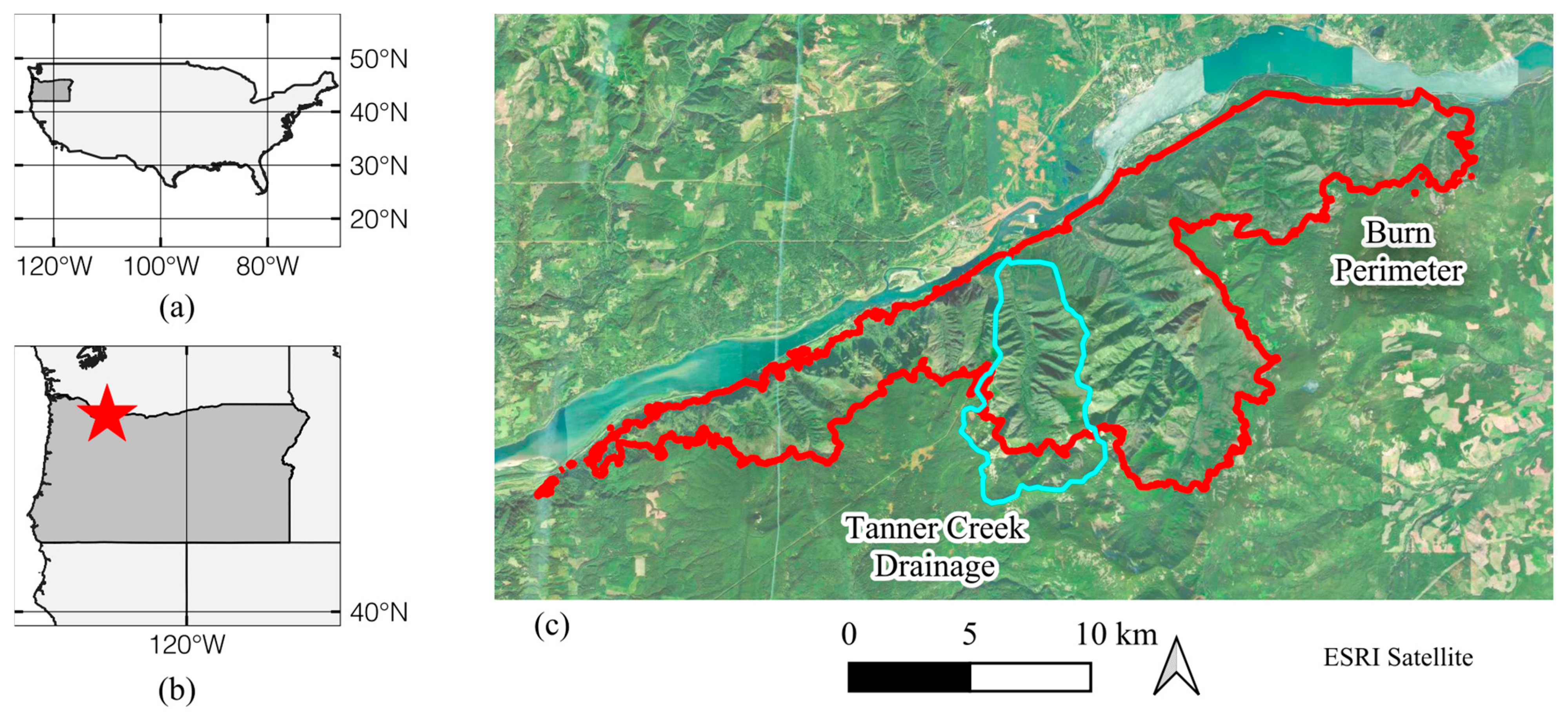
The focus of this study is to investigate the feasibility of using small-baseline subset differential interferometric synthetic aperture radar (SBAS-DInSAR) to interpret changes in ground surface elevation following large wildfires, with a specific application to the Tanner Creek drainage basin in northwestern Oregon, which experienced severe burning from the Eagle Creek Fire in 2017. We assess the temporal changes in the distribution or the estimated displacement, the spatial interferometric coherence, and explore connections to precipitation, soil moisture, and burn severity.

2. Wildfire Site and Geological Setting

The Eagle Creek Fire occurred in 2017, predominantly in the US state of Oregon, burning an estimated 200 km² between its initiation in early September and its declared containment in late November [25]. The wildfire perimeter delineated in Figure 1 is in a mountainous and landslide-prone region in the Mark O. Hatfield Wilderness, adjacent to both the Columbia River and the Historic Columbia River Highway to the north and the Mount Hood National Forest to the South. It is a popular outdoor destination, with extensive hiking trails and several scenic waterfalls. The area that burned experiences a wide range of precipitation in the form of snow and rainfall, much of which occurs between October and May. The area has numerous drainages with frequent debris flow activity, usually following rain-on-snow events. The steep, incised inner gorges of the Columbia River Basalt are subject to rapid weathering and frequent erosion, resulting in numerous landslides and sediment recruitment into channels below, resulting in perennial debris flow hazards. Bedrock geology at the site is predominantly basalt belonging to the Grande Ronde and Northwest Cascade Volcanoes formations [26]. Surficial conditions consist of exposed weathered rock, soils, and steep talus slopes. Vegetation is predominantly thick Douglas Fir forests. Elevations in the Tanner Creek drainage basin, which encompasses approximately 37.1 square kilometers, range from approximately 30 m to 1330 m.

The burn resulted in the 80-day closure of more than 120 miles of National Forest System hiking trails and 10 km of the Historic Columbia River Highway to allow for the removal of unstable trees along the highway [25]. Following the fire, a multi-agency group known as Monitoring Trends in Burn Severity (MTBS) and the Burned Area Emergency Response team (BAER) [27] evaluated the extent and severity of soil burning at the site of the Eagle Creek fire. Along with on-the-ground inspection, the group leverages satellite imagery from Landsat satellites and imagery from Sentinel-2 from before and after the fire, to determine the extent and severity of the fire on the landscape, particularly as it relates to changes in vegetation. Satellite observations were compared with limited field survey of ground conditions. Aerial imagery obtained from the Oregon Statewide Imagery Program (OSIP) before (2016) and after the fire (2018) demonstrates the effect on tree cover, both in the steep slopes adjacent to the Columbia River and in the mountainous central region of the burn perimeter. Figure 2 shows the ortho imagery taken before and after the fire alongside the burn severity map to demonstrate the effect of the fire on the vegetation coverage.

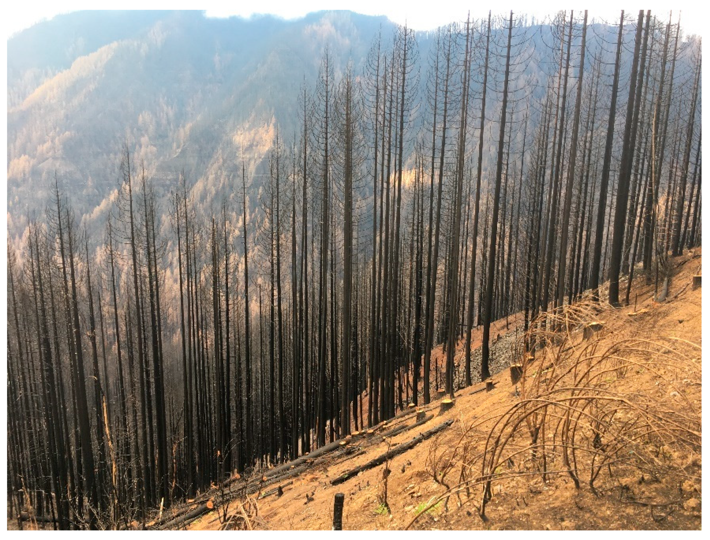
The MTBS and BAER survey determined that the central region, comprising the Eagle Creek and Tanner Creek drainage basins, was the most severely burned area with an estimated ground vegetation recovery time in these two drainage basins of 5–10 years [27]. Figure 3 shows a photograph of a burned slope in the Tanner Creek drainage basin taken after the fire, demonstrating the steepness of the terrain and extent of burning [28]. Generally, soils subjected to higher burn severity have reduced infiltration, thus increasing the likelihood of surface erosion, debris flows, and landslides [25]. However, in the cool and wet climate of Oregon, it is less clear as to the long-term effects severe wildfire pose as it relates to the timescales of change stemming from landslides, erosion and debris flows at large scales—DInSAR may serve as a means for quantifying these changes at short- and medium-timescales.

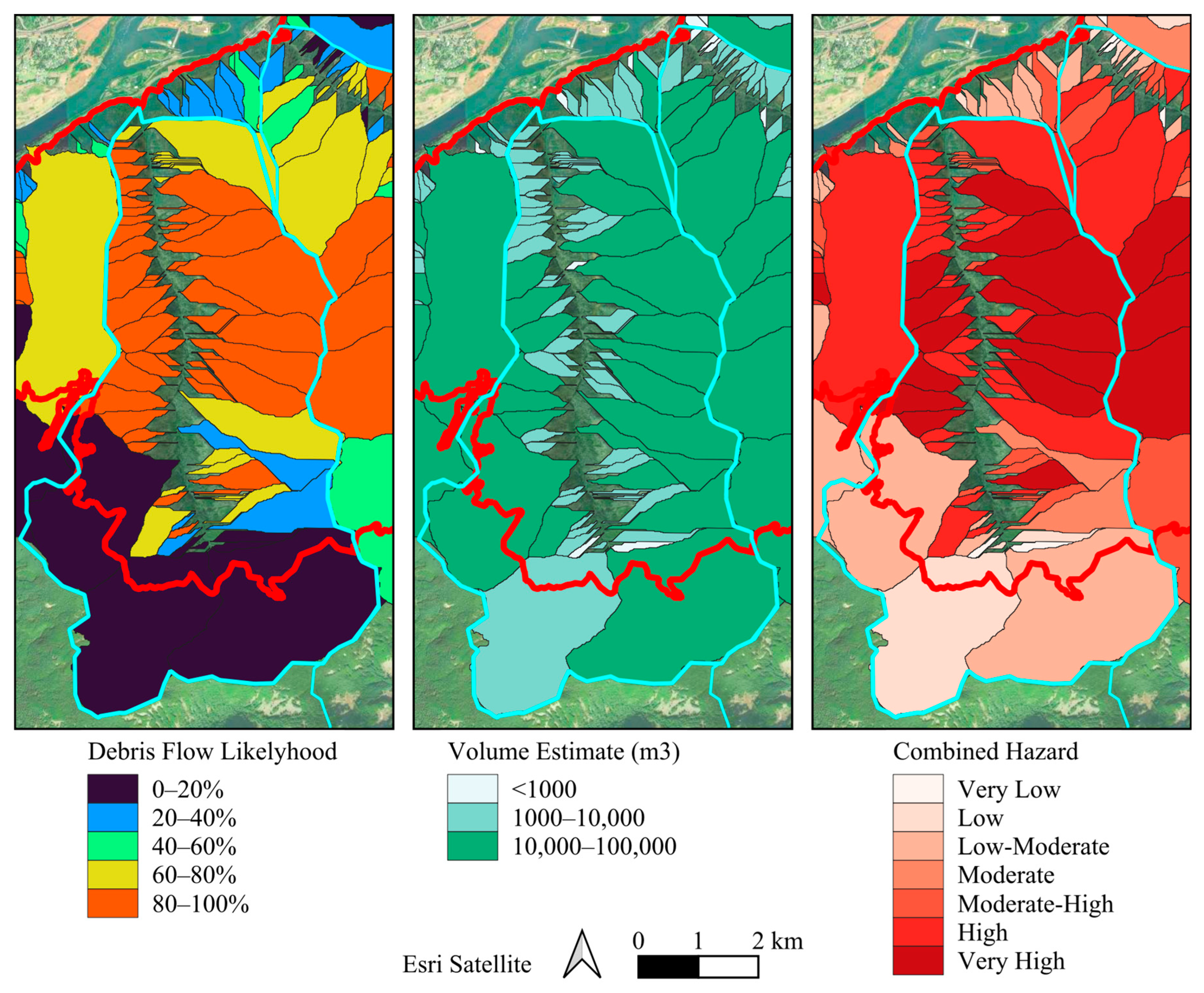
Burn severity and soil burn severity are important components of the US Geological Survey’s current models for estimating the likelihood and volume of debris flow in post-wildfire landscapes [29]. The preliminary hazard assessment comprises both a debris flow likelihood model based on logistic regression and a volume estimate model that uses multiple linear regression; outputs from these two models are ranked and summed to produce a combined hazard rating for each subbasin within the burn perimeter. The likelihood model is based on the proportion of upslope area burned to a certain severity, the average differenced normalized burn ratio (dNBR) in the upslope area, and soil erodibility. The volume estimate model is based on the range of elevations within the basin and the upstream burned area [29]. Parameters in the two models are based on empirical case histories of wildfires in the Western United States. Likelihood and volume estimates are made for several precipitation events defined by a peak 15 min intensity ranging from 12 to 40 mm/h [30]. Volume is estimated at the drainage basin-scale using the elevation range within the basin, the upstream area burned (moderate severity or higher), and the design peak 15 min rainfall intensity. Volume estimates are shown in Figure 4 and categorized into three categories: “low”, 0–1000, “medium” 1000–10,000, “high” 10,000–100,000, and “very high” > 100,000 m³. These USGS models are specific to recently burned areas in the Western United States.

While useful, this model is a one-time estimation based on previous case histories and does not necessarily consider the local-scale hydrological and ecological intricacies of a particular burn region, regrowth of vegetation, or the potential impacts of evolving hydrologic conditions in the years following a fire. By using spaceborne optical or radar image products, such as DInSAR, a method for continual monitoring of burned areas could contribute to hazard mitigation by providing regularly updated measurements of site-specific ground surface changes.

3. Methods

Data from the European Space Agency’s Sentinel-1 A satellite was used in this study. Sentinel-1 A is equipped with a C-band microwave sensor that has a wavelength of approximately 5.55 cm. [31]. C-band is well-suited for measuring changes in ground elevation in areas with low to moderate vegetation cover that, in general, have high coherence compared to densely forested area [32]. C-band radiation only partially penetrates forest canopies, resulting in volume scattering and decorrelation of the phase signal in heavily forested areas. In fact, heavy vegetation and tree cover is one of the main limitations of C-band SAR. The circumstances of this study, however, make C-band SAR applicable where it typically would not be, since the wildfire removed vegetation from many areas within the Tanner Creek drainage basin. Following the fire, the burned areas consisted of primarily of exposed soil and rock with limited surface vegetation, allowing for high coherence in these areas.

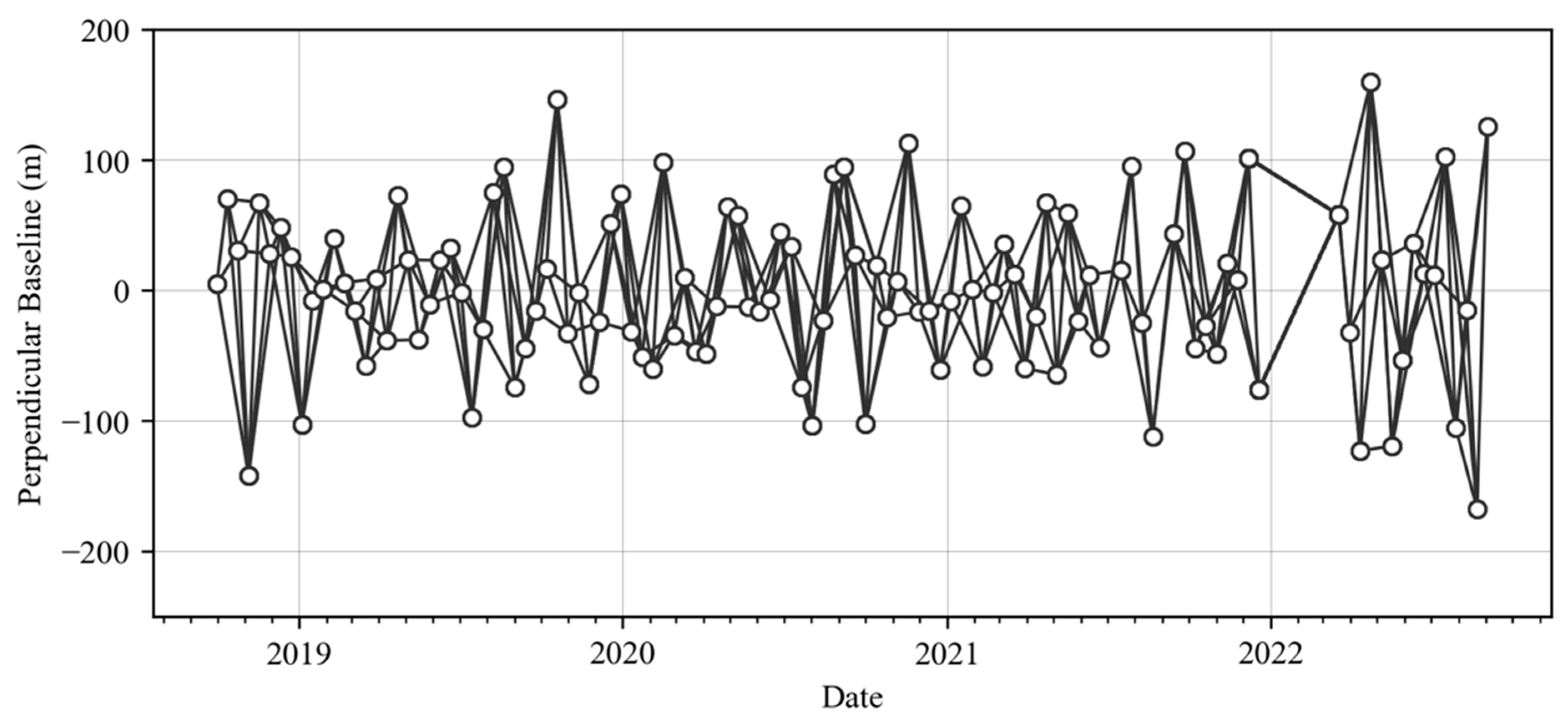
SAR imagery was obtained using Vertex, the Alaska Satellite Facility (ASF) data search application, to order on-demand Level-2 SAR imagery from the Sentinel-1 A satellite, ascending path 137, and processing with multi-look factor of 10 × 2 (range and azimuth directions) for a pixel size of approximately 38 m × 55 m in the range and azimuth directions, respectively. The ASF hosts NASA’s archive of SAR data and operates a suite of open-source processing tools in a cloud-computing environment, including OpenSARLab [33]. Interferogram pairs were generated using a temporal baseline (time between acquisitions) of 12 to 36 days, except in one case where pairs were manually created with longer temporal baselines due to unavailable interferograms: 19 December 2021–19 March 2022 (temporal baseline of 90 days). The temporal and perpendicular baselines of all acquisition pairs are shown in Figure 5. Interferograms were obtained from NASA’s SAR DAAC for a four-year period spanning approximate water years 2019 to 2022.

The data were brought into the OpenSARLab computing environment and processed following the SBAS technique using Miami InSAR Time-series Software in Python (MintPy, v1.60) [34]. Data pre-processing included creation and co-registration of image stacks resampled to the limits of the area of interest. The SBAS analysis, performed using MintPy, includes digital elevation model terrain corrections and tropospheric delay corrections and enables development of a displacement time series with high spatial density and extent using multiple chronologically acquired interferometric pairs.

MintPy starts with a stack of phase-unwrapped interferograms that have undergone correction for Earth curvature and topographic effects. All interferograms are then temporally referenced to the first image. The software then selects a spatial reference point by identifying and selecting a pixel with high average spatial coherence. After identifying temporal and spatial references, unwrapping error correction is applied utilizing the bridging of reliable regions as described in [35]. This method is particularly suited to regions with steep topography, such as the Tanner Creek drainage in this study. The interferogram network is then inverted before applying phase spatial coherence masking. The phase timeseries then undergoes correction for tropospheric delay using ERA-5 dataset and topographic errors using a digital elevation model (3-arc second SRTM DEM). Residual phase noise is then evaluated and removed before estimating line-of-site displacement and velocity. Refer to [34] for details on each processing step.

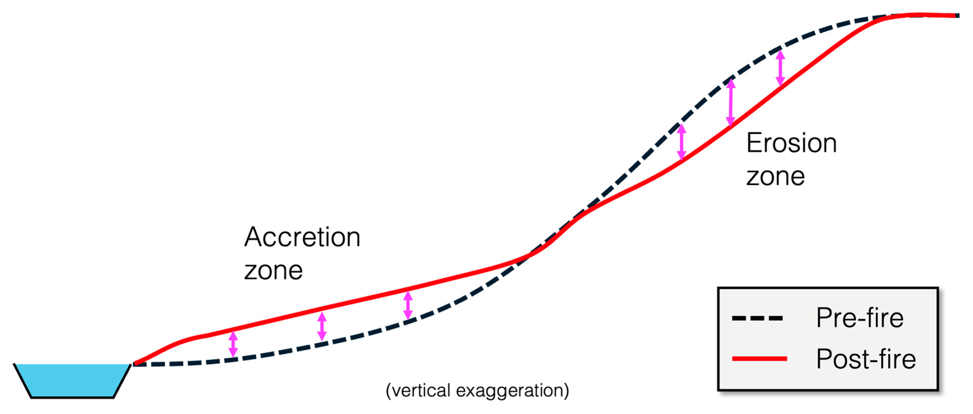
The time step of the timeseries depends on the repeat pass interval of the satellite being used and is 12 days for the Sentinel-1 A satellite used in this study. MintPy only supports single-track processing, thus only images from Sentinel-1 A along the same track were used. Line-of-sight (LOS) displacement was projected to vertical displacement using the following formula:

$$d_{LOS}=d_v\cos \left({\theta }_{inc}\right),$$

(1)

where $d_v$ is vertical displacement, $d_{LOS}$ is displacement in the LOS of the satellite, and ${\theta }_{inc}$ is the incident angle between the satellite look vector and a line normal to the ellipsoid. This projection assumes that all displacement observed by the satellite in the LOS direction is derived from vertical displacement of the ground surface and does not include a horizontal component. Consideration of the horizontal component is important in cases where slopes are moderate and the horizontal component may be significant, or where the ground surface displacements are a result of the movement of a large mass of soil (i.e., slow-moving landslides), or in cases where the phenomenon being measured occurs over a long timescale. In the Tanner Brook Drainage, the predominant driver of changes in the ground surface elevation is erosion following intense precipitation events, which occurs in intermittent and spatially distributed events. Additionally, these erosive events typically occur on a much shorter time scale than the repeat-pass interval of the satellite. Thus, the use of vertical projection is well suited to estimate changes in the ground surface resulting from these short-lived events. A schematic depicting this is shown in Figure 6.

Generally, coherence threshold of 0.2 to 0.3 is used in vegetated areas (see [2] where a coherence threshold of 0.3 was used to mask pixels in vegetated areas adjacent to the study are). The intent of a coherence threshold is to exclude pixels where decorrelation is significant and likely not a result of ground surface deformation, rather attributed to the effects of vegetation. In the Tanner Creek Drainage, many areas outside of the exposed slopes are densely forested and have low coherence. Low coherence in these areas increases uncertainty in the measured deformation. Since the objective of the study is to observe ground surface changes resulting from erosion in the exposed slopes, a coherence threshold of 0.5 was selected for this study which effectively masked adjacent vegetated areas and retained pixels within the exposed slopes burned to a high severity.

4. Results

The results are divided into two key findings: interferometric coherence threshold and investigation of ground surface changes.

4.1. Interferometric Coherence Threshold

Typically, DInSAR with the Sentinel-1 satellites is not effective in areas with dense forest or vegetation cover. The C-band microwave wavelength is unable to fully penetrate the canopy and interact with the ground surface, resulting in incoherent images. At Eagle Creek, the post-wildfire landscape offers a unique opportunity to apply C-band DInSAR techniques where they may not typically be applicable. The most heavily burned areas (i.e., Tanner Creek drainage basin) experienced effective removal of tree cover, leaving the ground surface exposed to the radar signal. For this reason, the interferometric coherence in areas burned with high severity is much higher than in low burn severity and unburned forested areas, as shown in Figure 7c,d, and as expected, coherence appears positively correlated with the burn severity class (i.e., lower coherence is associated with “moderate” and “low” burn severity) Figure 7b. Even areas of “moderate” burn severity located near the Tanner Creek have low coherence values. Figure 7e shows the distributions of average interferometric coherence in the Tanner Creek drainage for the 2019 water year, categorized by the MTBS burn severity class. This suggests that interferometric coherence may be a useful complement to traditional burn severity surveys, such as those conducted by MTBS using dNBR. It is important to note that the average interferometric coherence was computed for the entire water year (September-to-September) data stack. This is necessary to reduce decorrelation that is typical when comparing images acquired in different seasons.

In Figure 7c,d, spatial coherence is higher in the burned areas of the Tanner Creek drainage basins than in the surrounding unburned areas. There is an overall reduction in interferometric coherence from 2021 to 2022, possibly indicative of the effect of vegetation regrowth on signal scattering. However, areas that experienced a high burn severity still exhibit much higher coherence than other areas. Pixels belonging to the high burn severity class have the highest coherence values, while those belonging to the unburned to low class have the lowest—this is not surprising given that coherence is related to the surface cover/scattering, and high burn severity areas likely have less vegetation than low.

In general, the average annual interferometric coherence appears to separate areas that experienced “high” from “low” or “moderate” burn severity. For this reason, interferometric coherence may also be appropriate for developing a mask to exclude measurements from forested and unburned areas. A coherence threshold could be selected such that a mask is applied to all pixels with an average interferometric coherence below the threshold, where these pixels would not be considered when analyzing the SBAS results. Determining an appropriate interferometric coherence threshold was critical to maintaining the integrity of the results and identifying areas where interferometric phase changes are most likely due to ground surface displacements from areas where phase changes may be attributed to noise due to vegetation scattering. The coherence threshold should depend on the characteristics of the surface being imaged as well as the intent of the analysis. For example, if one intends to measure surface displacements, then a high coherence threshold may be appropriate for masking highly vegetated surfaces. Low coherence would likely be associated with phase error introduced due to scattering from the vegetation or changes in the vegetation between acquisitions.

Applying this coherence mask and projecting line-of-sight displacement to vertical displacement using Equation (1), we evaluated displacement during the 2018, 2019, 2020, and 2021 wet seasons (September to May) for three subbasins. The subbasins are shown individually Figure 8, with OSIP aerial imagery from 2016, 2018, and 2022 to demonstrate changes in vegetation throughout time and the MTBS burn severity map. Subbasins are also shown in the context of the greater drainage basin in Figure 9. Subbasin 1 was predominantly vegetated prior to the fire and consists almost entirely of “high” burn severity. Subbasin 2 was also predominantly vegetated prior to the fire and has some small talus slopes near the valley of the drainage basin; it consists mostly of “high” burn severity with a central area of “moderate” and “low”. Subbasin 3 was partially vegetated, with larger areas comprising talus slopes, and consisting almost entirely of “high” burn severity; it is adjacent to a subbasin that experienced low to no burn severity.

4.2. Ground Surface Changes

In general, most of the severe ground surface changes occurred in the two years following the fire. However, when subbasins were analyzed, not all areas experienced vertical displacement at the same time or rates. Examples of vertical displacement are plotted in Figure 9. For example, Subbasins 1 and 3 experienced generally significant erosion during the wet season of 2018–2019, while Subbasin 2 and adjacent subbasins experience little to no erosion or accretion. On soil and talus slopes, the ground surface displacements indicated by negative values are likely due to erosion and those indicated by positive values are likely due to accretion. From a mass balance perspective, it should be noted that material may be moving out of areas where measurements were retained and into areas excluded by the interferometric coherence mask. Figure 10 shows the distribution of projected vertical displacement for each year of the analysis.

Figure 11 shows a pre-fire ground surface profile from a DEM and a ground surface profile based on the projected vertical displacement that occurred from September 2018 to May 2019. Vertical displacement is exaggerated to show the centimeter-scale changes in the ground surface that were measured during this time.

The wet seasons from 2018 to 2019 and 2019–2020 experience the most significant displacements, except for a central region during the 2018–2019 period (see Subbasin 2) that does not show significant displacement. In general, slopes at higher elevation have greater negative deformation (erosion), with near zero or slightly positive deformations (accretion) occurring at lower elevations, suggesting a migration of material downslope. Figure 12 shows the relationship between projected vertical displacement and elevation in Subbasin 1. The color scale shows the dNBR at each measurement point.

In the Tanner Creek drainage, most of the interior steep slopes experienced high burn severity (see Figure 2c), except for areas at the perimeter of the burn area and those along the creek. For areas burned to a high severity (dNBR values greater than 660), there is a clear positive relationship between the dNBR and elevation, as shown in Figure 13. Lower elevations tend to contain more moisture, with higher elevations being dryer and thus more susceptible to more intense burning. In addition, fires tend to move rapidly up steep slopes as the rising hot air dries out the vegetation [36].

Precipitation data were obtained from the North Fork SNOTEL station 666, located approximately 7 km southwest of the Tanner Creek drainage basin at an elevation of 932 m; data are presented as cumulative precipitation throughout the water year in Figure 14. Soil moisture data, obtained using Google Earth Engine to query the SMAP L4 Global 3-hourly 9 km Root Zone Soil Moisture dataset [37], are estimated as the volume fraction of moisture in the upper 1 m of soil. Figure 14 also shows the vertical displacement of all InSAR pixels within Subbasins 1, 2, and 3 from September 2018 to September 2022.

The mean of projected vertical displacement, averaged over each interferogram acquisition date, is highlighted for each subbasin. Linear regressions were conducted on the mean displacement to estimate long-term displacement rates. These long-term regressions ignore sub-annual fluctuations, although in the case of Subbasin 2 two linear regressions were used (discussed later). Except for slight seasonal variations, Subbasin 1 appears to experience a steady displacement of −3.34 cm/yr on average. Subbasin 2 shows no trend in displacement from September 2018 to around January 2020. This is also apparent in Figure 9, which shows generally small vertical displacements compared to surrounding subbasins. Following January 2020, Subbasin 2 begins to experience vertical displacement rate of about −2.21 cm/yr Subbasin 3 shows a similar trend to Subbasin 1, displacing at a rate of about −2.64 cm/yr on average.

Generally, there appears to be a correlation between cumulative precipitation and erosion, with periods of precipitation corresponding to periods of increased erosion. Additionally, periods of lower soil moisture (i.e., June through October) align with slower or generally no erosion, while periods of higher soil moisture tend to align with the more rapid erosion. Figure 15 shows the relationship between precipitation, rootzone soil moisture, and projected vertical displacement (erosion) for the 2019 water year in Subbasin 1. Precipitation, soil moisture, and projected vertical displacement datasets are linked by the date of the InSAR acquisition. From the start of the water year, there appears to be a lag of about one month until the initiation of significant ground surface displacements (erosion). During this time, the rate of precipitation accumulation is generally steady, and rootzone soil moisture increases at a steady rate. The increased rate of ground surface deformation begins shortly before the peak of rootzone soil moisture. Once the rate of accumulated precipitation decreases, and rootzone soil moisture also decreases, toward the later third of the water year, a decrease in the rate of ground surface deformation can be observed.

There appears to be a lag from when precipitation begins to when there is a significant increase in the rootzone soil moisture rate of erosion. As can be seen in Figure 15, erosion begins to increase rapidly after about 1 m of accumulated precipitation; rootzone soil moisture is also at its highest during this period. Combining all four study years (2019–2022), there is a clear relationship between the accumulated precipitation and erosion in Subbasin 1, shown in Figure 16, which suggests a mean rate of erosion of −0.014 m per 1 m of accumulated precipitation over this time frame.

Similar trends were observed during the 2020, 2021, and 2022 water years and at all three subbasins.

5. Discussion

Advances in the application of new data, technologies, and tools are accelerated when barriers to access are reduced or removed. DInSAR offers many favorable characteristics for hazard monitoring, and the ability to freely access SAR data and process it using state-of-the-art algorithms and techniques in a cloud-based computing environment offers tremendous opportunity to expand its uses in hazard monitoring and potentially landscape recovery following wildfire.

The ability of SAR with the Sentinel-1 A satellite to make consistent measurements at an approximate 12-day repeat pass interval over a very large area is one of the greatest draws of this technology for hazard monitoring. This is especially relevant in the context of post-wildfire monitoring, where the affected area is often large and generally difficult to access. Deployment of traditional in situ instrumentation, such as GPS stations or inclinometers, or surveying of the area using traditional ground-based survey, LiDAR, and/or photogrammetry can be cost-prohibitive and infeasible. It would be unreasonable to, for example, fly LiDAR every 12 days for many years over a site of several square kilometers. One limitation of DInSAR in this regard is that the spatial resolution may not be fine enough to capture refined details in some smaller sites. Additionally, in some cases the 12-day repeat pass interval may not be a fine enough temporal resolution to capture short-term critical events. While longer-term phenomena, such as erosion, accretion, and vegetation regrowth can be captured with this temporal measurement interval, the progression of short-term phenomena such as a sudden movement of material (i.e., debris flows, landslides) may not be captured, except before and after.

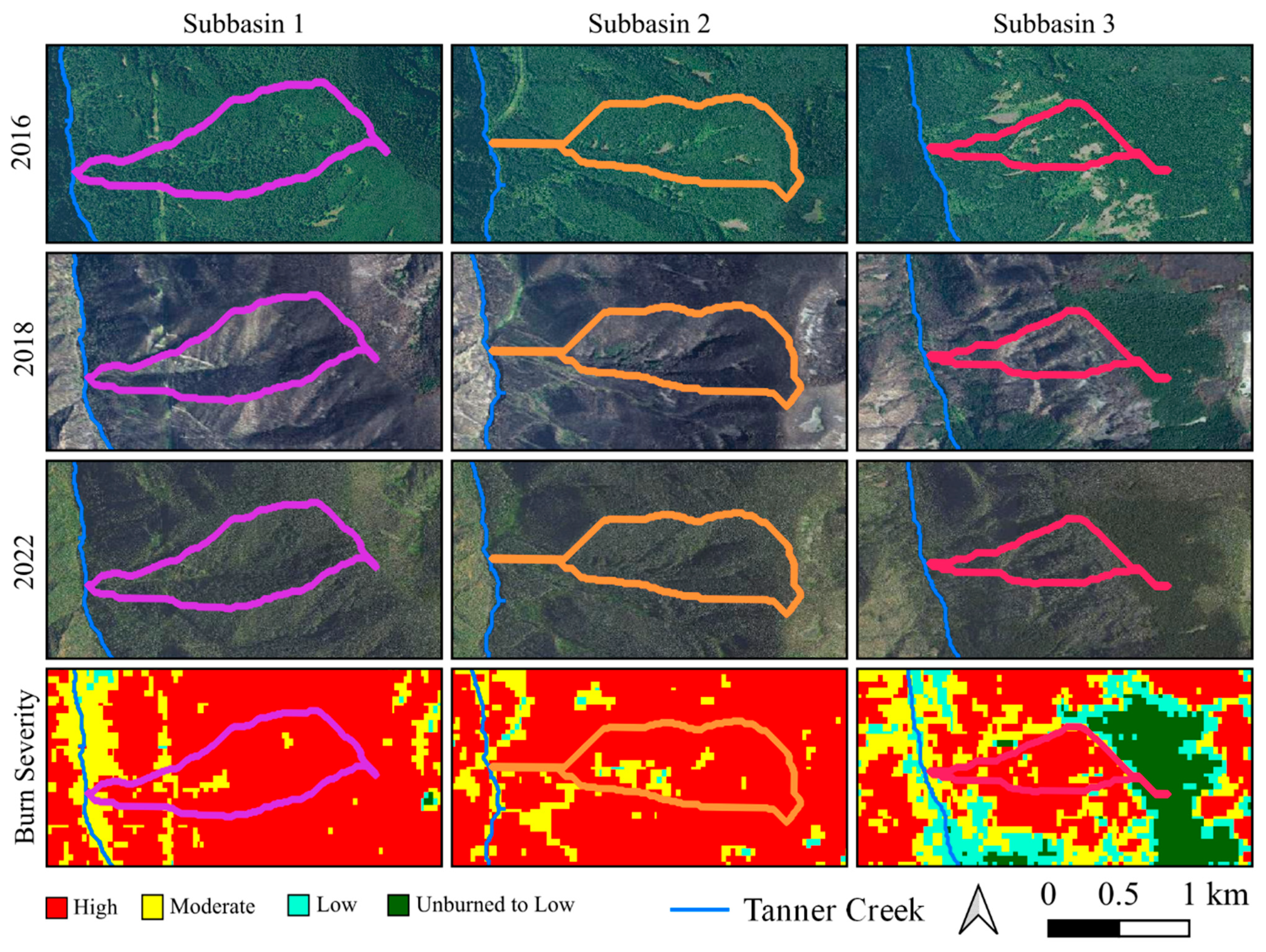
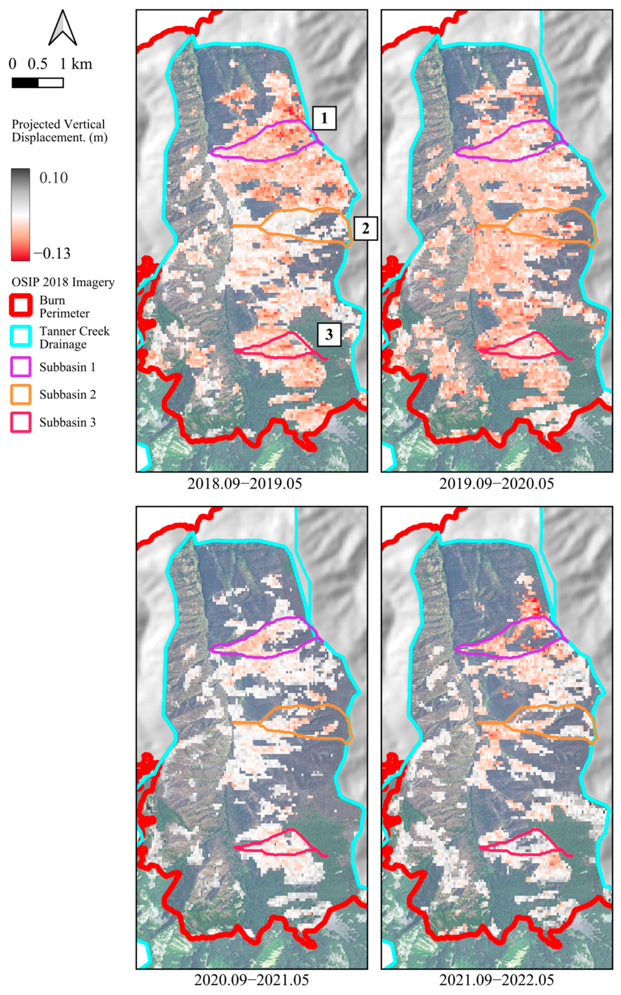
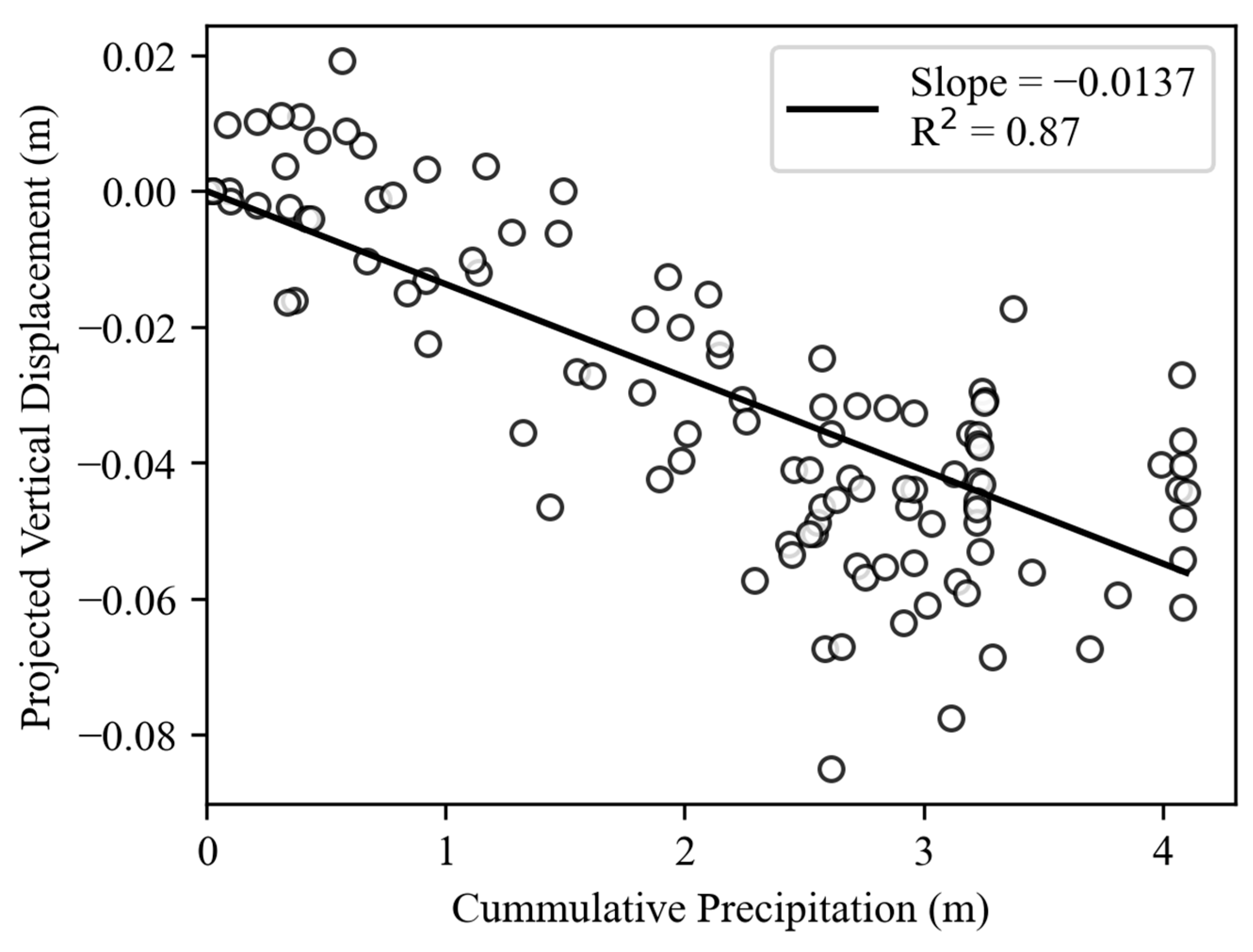
Rainfall is the principal driver of slope instabilities such as erosion or shallow landslides; significant wildfires change the near-surface hydrologic cycle and create conditions that can exacerbate the effects of rainfall and increase the quantity and intensity of runoff. Thus, establishing a connection between rainfall quantity and ground surface changes is important. We found that the three subbasins in the Tanner Creek drainage investigated in this study showed a strong connection between accumulated precipitation throughout the water year, rootzone soil moisture, and ground surface deformation. We found that there appears to be a lag between the initiation of precipitation at the start of the water year and the initiation of ground surface deformations. This is observed for all four water years covered in this study (2019–2022) when compared to the long-term time series of projected vertical displacement at the three subbasins (see Figure 14). We also found an increased rate in the ground surface deformation during periods of elevated rootzone soil moisture (see Figure 15) and a strong relationship between cumulative precipitation and ground surface deformation (see Figure 16).

The use of SAR for post-wildfire hazard monitoring is not without its limitations. Firstly, as mentioned above, the area being monitored may be devoid of existing instrumentation (i.e., GPS stations) that could be used to verify the DInSAR measurements. Of course, it is an asset of remote sensing, in general, that measurements can be made at un-monitored locations, and studies using DInSAR in monitored locations have shown good reliability of the technique as discussed earlier. If limited in situ monitoring is an option, DInSAR could first be used to assess potential locations for deployment of sensors to help ensure they are optimally located in critical areas.

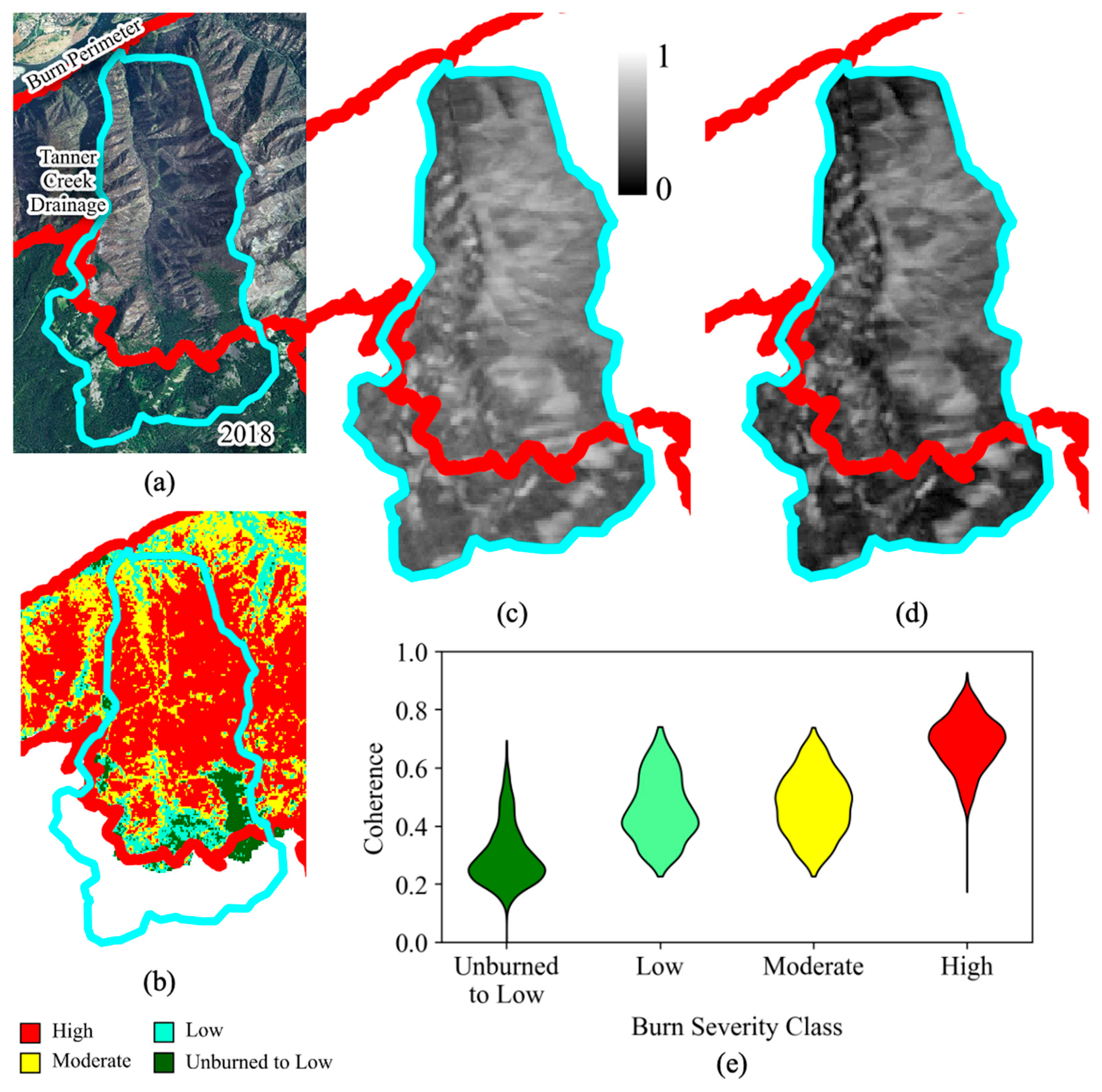
The interferometric coherence also shows strong potential for use in both masking unburned areas and in monitoring vegetation regrowth over time. Vegetation regrowth will limit the measurable area over time due to decreases in interferometric coherence. This effect is observed in Figure 9 where the area covered by coherent pixels decreases with time from the wildfire or disturbance. Thus, use of DInSAR for post-wildfire hazard monitoring is potentially limited by the rate of vegetation regrowth. In many cases, the vegetation regrowth period, and areas that experience high burn severity, may maintain relatively high coherence (e.g., Figure 7c,d) for several years to a decade; so, DInSAR may still be useful for some years. As demonstrated in Figure 7e, interferometric coherence is related sensitive to the burn severity and the presence of vegetation; therefore, it could be a valuable asset for monitoring of regrowth of vegetation following a wildfire and could be used as a complement to the dNBR.

6. Conclusions

This study used DInSAR techniques to analyze ground surface displacements in a severely burned drainage basin following the Eagle Creek Fire in 2017. An interferometric coherence mask was used to exclude readings from low burn severity and unburned areas that contained dense vegetation and tree cover, and coherence appears to be related to the burn severity class. Projected vertical displacement in the drainage basin and long-term displacement trends in three subbasins were analyzed.

Specific to the study site, the findings suggest that there is a window of vulnerability after a wildfire where ground surface deformations are higher—in this case the most significant measured erosion occurred two years after the fire. Some areas continued to show erosion at a consistent rate even beyond this three-year period. Observations of the spatial distribution of ground surface displacements indicated that the magnitude of erosion varied within the drainage basin, with some areas showing little to no ground surface displacement for up to four years after the fire. Comparison of ground surface displacement to precipitation and soil moisture suggested that trends in increased precipitation and increased soil moisture are generally consistent with the computed accelerated erosion. There appears to be a lag between the initiation of precipitation at the start of the water year and the initiation of ground surface deformations. This lag period of approximately one month is associated with a steady increase in the rootzone soil moisture.

References

1. Rathje, E.M.; Franke, K. Remote Sensing for Geotechnical Earthquake Reconnaissance. Soil Dyn. Earthq. Eng. 2016, 91, 304–316. [Google Scholar] [CrossRef]
2. Delbridge, B.G.; Bürgmann, R.; Fielding, E.; Hensley, S.; Schulz, W.H. Three-dimensional Surface Deformation Derived from Airborne Interferometric UAVSAR: Application to the Slumgullion Landslide. J. Geophys. Res. Solid Earth 2016, 121, 3951–3977. [Google Scholar] [CrossRef]
3. Kean, J.W.; Smith, J.B.; Rengers, F.K.; McGuire, L.A.; Staley, D.M. Post-Wildfire Debris-Flow Monitoring Data, Las Lomas, 2016 Fish Fire, Los Angeles County, California, November 2016 to February 2017; U.S. Geological Survey Data Release: Reston, VA, USA, 2019. [Google Scholar] [CrossRef]
4. Rengers, F.K.; McGuire, L.A.; Oakley, N.S.; Kean, J.W.; Staley, D.M.; Tang, H. Landslides after Wildfire: Initiation, Magnitude, and Mobility. Landslides 2020, 17, 2631–2641. [Google Scholar] [CrossRef]
5. Ferretti, A.; Prati, C.; Rocca, F. Permanent scatterers in SAR interferometry. IEEE Trans. Geosci. Remote Sens. 2001, 39, 8–20. [Google Scholar] [CrossRef]
6. Crosetto, M.; Monserrat, O.; Cuevas-González, M.; Devanthéry, N.; Crippa, B. Persistent Scatterer Interferometry: A review. ISPRS J. Photogramm. Remote Sens. 2016, 115, 78–89. [Google Scholar] [CrossRef]
7. Domínguez-Cuesta, M.J.; Rodríguez-Rodríguez, L.; López-Fernández, C.; Pando, L.; Cuervas-Mons, J.; Olona, J.; González-Pumariega, P.; Serrano, J.; Valenzuela, P.; Jiménez-Sánchez, M. Using Remote Sensing Methods to Study Active Geomorphologic Processes on Cantabrian Coastal Cliffs. Remote Sens. 2022, 14, 5139. [Google Scholar] [CrossRef]
8. Ferretti, A.; Fumagalli, A.; Novali, F.; Prati, C.; Rocca, F.; Rucci, A. A New Algorithm for Processing Interferometric Data-Stacks: SqueeSAR. IEEE Trans. Geosci. Remote Sens. 2011, 49, 3460–3470. [Google Scholar] [CrossRef]
9. Casu, F.; Manconi, A.; Pepe, A.; Motagh, M.; Shamshiri, R.; Haghighi, M.H.; Wetzel, H.-U.; Akbari, B.; Nahavandchi, H.; Roessner, S.; et al. Deformation Time-Series Generation in Areas Characterized by Large Displacement Dynamics: The SAR Amplitude Pixel-Offset SBAS Technique. IEEE Trans. Geosci. Remote Sens. 2011, 49, 2752–2763. [Google Scholar] [CrossRef]
10. Berardino, P.; Fornaro, G.; Lanari, R.; Sansosti, E. A New Algorithm for Surface Deformation Monitoring Based on Small Baseline Differential SAR Interferograms. IEEE Trans. Geosci. Remote Sens. 2002, 40, 2375–2383. [Google Scholar] [CrossRef]
11. Handwerger, A.L.; Huang, M.H.; Fielding, E.J.; Booth, A.M.; Bürgmann, R. A shift from drought to extreme rainfall drives a stable landslide to catastrophic failure. Sci. Rep. 2019, 9, 1569. [Google Scholar] [CrossRef]
12. Handwerger, A.L.; Roering, J.J.; Schmidt, D.A. Controls on the Seasonal Deformation of Slow-Moving Landslides. Earth Planet. Sci. Lett. 2013, 377–378, 239–247. [Google Scholar] [CrossRef]
13. Hilley, G.E.; Bürgmann, R.; Ferretti, A.; Novali, F.; Rocca, F. Dynamics of slow-moving landslides from permanent scatterer analysis. Science 2004, 304, 1952–1955. [Google Scholar] [CrossRef] [PubMed]
14. Manconi, A.; Kourkouli, P.; Caduff, R.; Strozzi, T.; Loew, S. Monitoring Surface Deformation over a Failing Rock Slope with the ESA Sentinels: Insights from Moosfluh Instability, Swiss Alps. Remote Sens. 2018, 10, 672. [Google Scholar] [CrossRef]
15. Shirzaei, M.; Bürgmann, R. Global Climate Change and Local Land Subsidence Exacerbate Inundation Risk to the San Francisco Bay Area. Sci. Adv. 2018, 4, eaap9234. [Google Scholar] [CrossRef]
16. Shirzaei, M.; Freymueller, J.; Törnqvist, T.E.; Galloway, D.L.; Dura, T.; Minderhoud, P.S.J. Minderhoud. Measuring, Modelling and Projecting Coastal Land Subsidence. Nat. Rev. Earth Environ. 2020, 2, 40–58. [Google Scholar] [CrossRef]
17. Motagh, M.; Shamshiri, R.; Haghighi, M.H.; Wetzel, H.-U.; Akbari, B.; Nahavandchi, H.; Roessner, S.; Arabi, S. Quantifying groundwater exploitation induced subsidence in the Rafsanjan plain, southeastern Iran, using InSAR time-series and in situ measurements. Eng. Geol. 2017, 218, 134–151. [Google Scholar] [CrossRef]
18. Khorrami, M.; Shirzaei, M.; Ghobadi-Far, K.; Werth, S.; Carlson, G.; Zhai, G. Groundwater Volume Loss in Mexico City Constrained by InSAR and GRACE Observations and Mechanical Models. Geophys. Res. Lett. 2023, 50, e2022GL101962. [Google Scholar] [CrossRef]
19. Zhai, G.; Shirzaei, M.; Manga, M. Widespread Deep Seismicity in the Delaware Basin, Texas, Is Mainly Driven by Shallow Wastewater Injection. Proc. Natl. Acad. Sci. USA 2021, 118, e2102338118. [Google Scholar] [CrossRef] [PubMed]
20. Ponziani, F.; Ciuffi, P.; Bayer, B.; Berni, N.; Franceschini, S.; Simoni, A. Regional-Scale InSAR Investigation and Landslide Early Warning Thresholds in Umbria, Italy. Eng. Geol. 2023, 327, 107352. [Google Scholar] [CrossRef]
21. Jimeno-Llorente, L.; Marcos, E.; Fernández-Guisuraga, J.M. The Effects of Fire Severity on Vegetation Structural Complexity Assessed Using SAR Data Are Modulated by Plant Community Types in Mediterranean Fire-Prone Ecosystems. Fire 2023, 6, 450. [Google Scholar] [CrossRef]
22. Ebel, B.A.; Moody, J.A. Parameter Estimation for Multiple Post-wildfire Hydrologic Models. Hydrol. Process. 2020, 34, 4049–4066. [Google Scholar] [CrossRef]
23. Vahedifard, F.; Abdollahi, M.; Leshchinsky, B.A.; Stark, T.D.; Sadegh, M.; AghaKouchak, A. Interdependencies between wildfire-induced alterations in soil properties, near-surface processes, and geohazards. Earth Space Sci. 2024, 11, e2023EA003498. [Google Scholar] [CrossRef]
24. Abdollahi, M.; Vahedifard, F.; Tracy, F.T. Post-Wildfire Stability of Unsaturated Hillslopes Against Rainfall-Triggered Landslides. Earth’s Future 2023, 11, e2022EF003213. [Google Scholar] [CrossRef]
25. USDA Forest Service. At-A-Glance Facts, May 2018. In Eagle Creek Fire Fact Sheet; USDA Forest Service: Lakewood, CA, USA, 2018. [Google Scholar]
26. Korosec, M.A. Washington Department of Natural Resources Open-File Report 87-6, Scale 1:100,000. In Geologic Map of the Hood River Quadrangle, Washington and Oregon; Washington State Department of Natural Resources: Olympia, WA, USA, 1987. [Google Scholar]
27. Monitoring Trends in Burn Severity. May 2023. Available online: https://burnseverity.cr.usgs.gov/products/mtbs (accessed on 7 October 2023).
28. Sobieszczyk, S. View Along a Bluff in Tanner Creek Watershed Following the 2017 Eagle Creek Fire, Oregon (Columbia Gorge). Photograph. Oregon Water Science Center. Public Domain. Available online: https://www.usgs.gov/media/images/tanner-creek-after-eagle-creek-fire-oregon (accessed on 16 October 2023).
29. USGS Landslide Hazards Program. The Scientific Background Information for Emergency Assessment of Post-Fire Debris-Flow Hazards. Available online: https://www.usgs.gov/programs/landslide-hazards/science/scientific-background#overview (accessed on 7 October 2023).
30. Staley, D.M.; Negri, J.A.; Kean, J.W.; Laber, J.L.; Tillery, A.C.; Youberg, A.M. Updated Logistic Regression Equations for the Calculation of Post-Fire Debris-Flow Likelihood in the Western United States. In USGS Open-File Report 2016-1106; US Geological Survey (USGS): Reston, VA, USA, 2016. [Google Scholar]
31. European Space Agency. Sentinel-1 SAR User Guide. Available online: https://sentiwiki.copernicus.eu/web/document-library#Library-S1-Documents (accessed on 30 January 2023).
32. Flores, A.; Herndon, K.; Thapa, R.; Cherrington, E. Comprehensive Methodologies for Forest Monitoring and Biomass Estimation. In Synthetic Aperture Radar (SAR) Handbook; NTRS: Hampton, VA, USA, 2019. [Google Scholar] [CrossRef]
33. Alaska Satellite Facility. Available online: https://asf.alaska.edu/asf/about-asf/ (accessed on 30 January 2023).
34. Yunjun, Z.; Fattahi, H.; Amelung, F. Small baseline InSAR time series analysis: Unwrapping error correction and noise reduction. Comput. Geosci. 2019, 133, 104331. [Google Scholar] [CrossRef]
35. Chen, C.W.; Zebker, H.A. Phase unwrapping for large SAR interferograms: Statistical segmentation and generalized network models. IEEE Trans. Geosci. Remote Sens. 2002, 40, 1709–1719. [Google Scholar] [CrossRef]
36. Harris, L.; Taylor, A.H. Previous burns and topography limit and reinforce fire severity in a large wildfire. Ecosphere 2017, 8, e02019. [Google Scholar] [CrossRef]
37. Reichle, R.H.; Lannoy, G.D.; Koster, R.D.; Crow, W.T.; Kimball, J.S.; Liu, Q.; Bechtold, M. SMAP L4 Global 3-hourly 9 km EASE-Grid Surface and Root Zone Soil Moisture Analysis Update, Version; NASA National Snow and Ice Data Center Distributed Active Archive Center: Boulder, CO, USA, 2022. [Google Scholar] [CrossRef]
Figure 1. (a) The continental United States showing the state of Oregon; (b) state of Oregon with location of Eagle Creek fire indicated by star; (c) burn perimeter of the Eagle Creek Fire (shown in red) and location of the Tanner Creek drainage basin (shown in cyan).
Remotesensing 17 02047 g001
Figure 2. OISP ortho imagery of the Tanner Creek drainage basin (a) before the fire in 2016; (b) after the fire in 2018; (c) MTBS burn severity map developed after the fire [27].
Remotesensing 17 02047 g002
Figure 3. Photograph of a burned slope in the Tanner Creek drainage basin taken in 2018. Part of the slope is vegetated, and part is covered in talus (see far side of slope). (Source: [28]).
Remotesensing 17 02047 g003
Figure 4. Example of USGS models estimates of debris flow likelihood, flow volume, and combined hazard rating in the Tanner Creek drainage basin for a precipitation event with a 15 min peak intensity of 20 mm/h (Source: [29,30]).
Remotesensing 17 02047 g004
Figure 5. Perpendicular and temporal baseline of InSAR image pairs.
Remotesensing 17 02047 g005
Figure 6. Schematic depicting the use of vertical projection for estimating changes in the ground surface elevation.
Remotesensing 17 02047 g006
Figure 7. (a) Tanner Creek drainage basin in 2018 after the fire; (b) the MTBS burn severity map; average spatial coherence from (c) September 2018 to 2019; and (d) September 2021 to 2022; (e) Distribution of average interferometric coherence for 2019, categorized by burn severity class.
Remotesensing 17 02047 g007
Figure 8. Ortho imagery (0.3 m resolution) of the Tanner Creek drainage basin from 2016 (pre-fire), 2018, and 2022 (both post-fire) with subbasins 1, 2, and 3 shown from left to right. Burn severity is also shown for reference. Blue line is the Tanner Creek. Purple, orange, and pink polygons are outlines of the three subbasins.
Remotesensing 17 02047 g008
Figure 9. Vertical displacement during the wet season (September to May) for 2018 through 2022. The number of coherent pixels (masked at average coherence of 0.51) decreases with time, likely due to regrowth of surface vegetation. Base ortho imagery is from 2018.
Remotesensing 17 02047 g009
Figure 10. Boxplots showing the distribution of vertical displacement in the Tanner Creek drainage basin with a coherence mask threshold = 0.51 as shown in Figure 9. There appears to be a significant decrease in vertical displacement between the 2019–2020 and 2020–2021 wet seasons.
Remotesensing 17 02047 g010
Figure 11. (a) Location of surface profile (green line); (b) surface profile from Subbasin 1 showing pre-fire ground surface as determined from a DEM (black line, shown right) and vertically exaggerated ground surface profile (dashed red line) following the 2018–2019 wet season. The DEM has a pixel spacing of 40 m × 40 m. The surface profile is exaggerated by ×1000 in the vertical to ensure the centimeter-scale displacements are visible.
Remotesensing 17 02047 g011
Figure 12. Relationship between projected vertical displacement, elevation, and dNBR in Subbasin 1. Projected vertical displacement is for the 2018–2019 wet season. A dNBR greater than about 440 is generally considered moderate or higher burn severity.
Remotesensing 17 02047 g012
Figure 13. Relationship between dNBR and elevation for areas burned to a high severity (dNBR > 660).
Remotesensing 17 02047 g013
Figure 14. (top) Cumulative precipitation over water year from nearby SNOTEL station, vertical dashed gray line indicates start of new water season; (middle) SMAP rootzone soil moisture; (bottom) projected vertical displacement timeseries, with linear regression on the mean displacement for corresponding subbasins locations shown (right).
Remotesensing 17 02047 g014
Figure 15. Relationship between cumulative precipitation, rootzone soil moisture, and projected vertical displacement for the 2019 water year, Subbasin 1.
Remotesensing 17 02047 g015
Figure 16. Relationship between accumulated precipitation and projected vertical displacement (erosion) in Subbasin 1 for water years 2019–2022.
Remotesensing 17 02047 g016
Disclaimer/Publisher’s Note: The statements, opinions and data contained in all publications are solely those of the individual author(s) and contributor(s) and not of MDPI and/or the editor(s). MDPI and/or the editor(s) disclaim responsibility for any injury to people or property resulting from any ideas, methods, instructions or products referred to in the content.