CSNet: A Remote Sensing Image Semantic Segmentation Network Based on Coordinate Attention and Skip Connections

Abstract

In recent years, the continuous development of deep learning has significantly advanced its application in the field of remote sensing. However, the semantic segmentation of high-resolution remote sensing images remains challenging due to the presence of multi-scale objects and intricate spatial details, often leading to the loss of critical information during segmentation. To address this issue and enable fast and accurate segmentation of remote sensing images, we made improvements based on SegNet and named the enhanced model CSNet. CSNet is built upon the SegNet architecture and incorporates a coordinate attention (CA) mechanism, which enables the network to focus on salient features and capture global spatial information, thereby improving segmentation accuracy and facilitating the recovery of spatial structures. Furthermore, skip connections are introduced between the encoder and decoder to directly transfer low-level features to the decoder. This promotes the fusion of semantic information at different levels, enhances the recovery of fine-grained details, and optimizes the gradient flow during training, effectively mitigating the vanishing gradient problem and improving training efficiency. Additionally, a hybrid loss function combining weighted cross-entropy and Dice loss is employed. To address the issue of class imbalance, several categories within the dataset are merged, and samples with an excessively high proportion of background pixels are removed. These strategies significantly enhance the segmentation performance, particularly for small-sample classes. Experimental results from the Five-Billion-Pixels dataset demonstrate that, while introducing only a modest increase in parameters compared to SegNet, CSNet achieves superior segmentation performance in terms of overall classification accuracy, boundary delineation, and detail preservation, outperforming established methods such as U-Net, FCN, DeepLabv3+, SegNet, ViT, HRNe and BiFormert.

1. Introduction

Remote sensing imagery contains extensive semantic information of ground objects, offering comprehensive and efficient data support for remote sensing information processing. Performing semantic segmentation on such imagery enables the precise extraction of surface object semantics, which has broad applications in land cover classification [1,2], urban planning [3,4,5], environmental monitoring [6,7], and disaster assessment [8].

Traditional machine learning methods, such as Support Vector Machines (SVMs) [9,10] and Random Forests [11,12], often require manually designed features for specific application scenarios when performing semantic segmentation on remote sensing images. This leads to slow computation on large-scale datasets, making it difficult to meet the demands of remote sensing tasks. In contrast, deep learning methods, particularly Convolutional Neural Networks (CNNs) [13], can automatically extract deep features from images, capture spatial contextual information, and model intrinsic relationships between pixels, thereby significantly improving both the accuracy and efficiency of semantic segmentation in computer vision. As the first deep learning model applied to semantic segmentation, Fully Convolutional Networks (FCNs) [14] introduced an end-to-end training paradigm that enables the automated transformation from input images to segmentation outputs. Subsequent models like U-Net [15], DeepLab [16,17] and HRNet [18] further enhanced the performance of remote sensing segmentation through various architectural innovations and optimization strategies [19,20,21,22,23,24]. Moreover, some studies have introduced skip connections into the SegNet architecture, though these approaches have primarily been applied in the medical imaging domain [25,26]. A study has incorporated an improved coordinate attention mechanism into U-Net for efficient semantic segmentation, aiming to enhance accuracy while reducing computational overhead [27]. However, its ability to accurately delineate object boundaries still requires further improvement.

Although CNNs have achieved remarkable progress in semantic segmentation over the past decade, their inherent inductive bias and limited receptive fields constrain their ability to capture long-range dependencies and global contextual information. This limitation becomes particularly evident when dealing with remote sensing imagery characterized by complex spatial patterns and large-scale structures. In recent years, Transformer-based models [28] have emerged as a new foundational model following CNNs. Compared to CNN-based models, Transformer-based models possess a global modeling capability thanks to self-attention mechanisms, which can effectively capture long-range dependencies and contextual information within images. Subsequently, numerous Transformer-based semantic segmentation methods have been developed, such as Vision Transformer (ViT) [29], Swin Transformer [30] and BiFormer [31], which have demonstrated excellent performance across multiple mainstream datasets, thereby fully showcasing the advantages of the Transformer architecture. However, in semantic segmentation tasks involving small-sized remote sensing images, the advantages of the Transformer architecture’s self-attention mechanism are less evident. Instead, the local receptive fields of traditional CNN architecture tend to yield better performance on such small-sized inputs [32].

Although the accuracy of semantic segmentation models has been steadily improving, in certain remote sensing application scenarios, such as UAV-based dynamic monitoring [33] and emergency disaster response [34], models often need to be deployed directly on devices like drones and perform real-time segmentation. These tasks not only require segmentation accuracy but also impose strict constraints on inference speed and parameter size. Therefore, it is crucial to design a semantic segmentation network that can strike a balance between accuracy and efficiency.

SegNet [35], originally proposed to meet the real-time demands of autonomous driving, employs an encoder–decoder architecture to balance accuracy and computational efficiency. The encoder of SegNet adopts a VGG16-like structure to progressively extract high-level features from the input image, while the decoder reconstructs the segmentation map at the original resolution through upsampling and layer-wise feature recovery. Notably, SegNet employs pooling indices to record the positions of maximum activations during downsampling, allowing the decoder to accurately restore the spatial structure in the upsampling process. This architectural design not only preserves fine-grained feature details but also enhances computational efficiency, making SegNet widely adopted in semantic segmentation tasks. However, in remote sensing tasks, there are significant differences between remote sensing images and natural images in terms of resolution and object size, and there is also considerable variation in the sizes of objects within remote sensing imagery. As a result, directly applying SegNet to remote sensing image semantic segmentation may lead to the loss of object detail information and poor segmentation performance for certain categories (see Supplementary Material for details).

Therefore, we propose an improved SegNet-based network aimed at enhancing the balance between accuracy and computational efficiency of semantic segmentation for remote sensing imagery. Our improvements focus on the following aspects:

• Incorporating the coordinate attention (CA) [36] mechanism: By adding a coordinate attention module in the encoder, we enhance the model’s ability to capture spatial and channel features, improving segmentation accuracy.
• Introducing the skip connection (SC) [15] mechanism: Skip connections are established between each encoder layer and its corresponding decoder layer, directly linking the deep features received by the decoder with the shallow features of the image. This fusion enables the decoder to better combine detailed information with semantic features, thus improving segmentation accuracy.
• Select an appropriate loss function: We adopt a hybrid loss function, which includes weighted cross-entropy loss and Dice coefficient loss, to improve the model’s ability to segment small sample categories and alleviate the class imbalance issue present in remote sensing images.

2. Materials and Methods

2.1. Overview of CSNet Architecture

The SegNet network is an end-to-end semantic segmentation network, consisting of two main parts: the encoder and the decoder, as shown in Figure 1. In the encoder, five max pooling layers and thirteen convolutional layers are grouped into five downsampling stages, with each downsampling stage containing two to three convolutional layers and a max pooling layer. Importantly, SegNet retains the pooling indices during the max pooling process, which encodes the positions of the maximum values in the input image. In the decoder part, there are also five upsampling layers and thirteen convolutional layers, maintaining symmetry with the encoder part. The image features extracted by the encoder are first upsampled using the pooling indices to restore the image size, followed by convolutional layers to recover the image features.

This paper addresses the need for semantic segmentation of remote sensing images and proposes an improved semantic segmentation network, named CSNet, based on the SegNet network. The key improvements include the introduction of a coordinate attention mechanism, the use of skip connections, and the selection of an appropriate loss function. The structure of the improved network is shown in Figure 2.

2.2. Coordinate Attention

The coordinate attention mechanism is designed to enhance the neural network’s ability to model spatial positional information while retaining channel information. The coordinate attention mechanism combines both spatial and channel information, allowing the model not only to focus on the important features but also to accurately capture the spatial position of the features. The structure of the coordinate attention mechanism is shown in Figure 3.

First, global average pooling is performed on the input feature map $\mathrm{X}$ with size $\mathrm{C}\times \mathrm{H}\times \mathrm{W}$ along the width and height dimensions to obtain two feature maps, respectively.

$$z_c^h\left(h\right)={\displaystyle \frac{1}{W}}{\sum }_{0\le i<W}{x}_c(h,i),$$

(1)

$$z_c^w\left(w\right)={\displaystyle \frac{1}{H}}{\sum }_{0\le j<H}{x}_c(j,w),$$

(2)

where $x_c$ represents the pixel values of channel $c$ in the feature map $\mathrm{X}$, and $z_c^h$ and $z_c^w$ represent the feature vectors in the two directions (height and width) of channel $c$, with $c$ ranging from 1 to $C$.

Then, the two feature maps $z^h$ and $z^w$ are concatenated to form the vector $[z^h,z^w]$, which is passed through a $1\times 1$ convolution transformation function $F_1$ to extract important features from the concatenated feature map. After that, a non-linear activation function $\mathsf{\delta }$ (usually Sigmoid) is applied to obtain the intermediate feature map $\mathrm{f}$.

$$\mathrm{f}=\mathsf{\delta }\left(F_1\right([z^h,z^w]\left)\right),$$

(3)

Then, $\mathrm{f}$ is split along the spatial dimensions into two independent tensors, ${\mathrm{f}}^h$ and ${\mathrm{f}}^w$. These tensors are then transformed through $1\times 1$ convolutional functions $F_h$ and $F_w$, followed by a Sigmoid activation function. The resulting tensors $g^h$ and $g^w$, with the same number of channels as the input, are used as attention weights.

$$g^h=\mathsf{\sigma }\left(F_h\right({\mathrm{f}}^h\left)\right),$$

(4)

$$g^w=\mathsf{\sigma }\left(F_w\right({\mathrm{f}}^w\left)\right)$$

(5)

The output $\mathrm{Y}$ of the attention mechanism can be expressed as follows:

$$y_c\left(i,j\right)=x_c(i,j)\times g_c^h\left(i\right)\times g_c^w\left(j\right)$$

(6)

where $y_c$, $x_c$, $g_c^h$, and $g_c^w$ represent the values of the corresponding tensors or vectors in channel $c$.

2.3. Skip Connection

Skip connection (SC) is a widely used structural enhancement technique in deep neural networks, establishing direct connection between corresponding parts of the encoder and decoder. In this study, the feature A maps obtained after the coordinate attention layer of encoder are concatenated with the upsampled feature maps B from the corresponding decoder blocks, resulting in the combined feature map [A, B]. The fused feature maps, with doubled channel dimensions, are then passed through convolutional layers to recover semantic features. For instance, assuming the input image has a size of 3 × 256 × 256, the first convolutional block in the encoder produces a 64 × 256 × 256 feature map before downsampling. In the corresponding decoder block, after upsampling, a 64 × 256 × 256 feature map is also obtained. These two feature maps are concatenated to form a 128 × 256 × 256 feature map, which is then passed through a convolutional layer for feature recovery, thereby completing the skip connection for the first convolutional block. This process is repeated for each convolutional block in the encoder to fully implement the skip connection architecture.

2.4. Loss Function

In remote sensing imagery, the distribution of land cover types is often highly imbalanced, with some categories occupying a small proportion of the image. To address this challenge, this paper combines weighted cross-entropy loss and Dice coefficient loss for the computation of the loss function. The formula for the combined loss is as follows:

$$\mathrm{L}\mathrm{o}\mathrm{s}\mathrm{s}=\mathrm{W}\mathrm{C}\mathrm{E}+\mathrm{D}\mathrm{i}\mathrm{c}\mathrm{e} \mathrm{L}\mathrm{o}\mathrm{s}\mathrm{s}$$

(7)

where $\mathrm{W}\mathrm{C}\mathrm{E}$ is the weighted cross-entropy loss [37,38], and $\mathrm{D}\mathrm{i}\mathrm{c}\mathrm{e} \mathrm{L}\mathrm{o}\mathrm{s}\mathrm{s}$ is the Dice coefficient loss [39,40].

2.4.1. Weighted Cross-Entropy Loss

Standard cross-entropy loss is a commonly used loss function in classification tasks, measuring the difference between the predicted probability distribution and the true distribution. It is essentially a form of negative log-likelihood, which penalizes incorrect classifications and encourages the model to output probabilities closer to the true labels. If we let the model’s predicted output be $p$ and the true label be $y$, the calculation formula for cross-entropy loss is as follows:

$$\mathrm{C}\mathrm{E}=-\sum _{c=1}^C{y}_c\log p_c$$

(8)

where $C$ is the number of classes, $p_c$ is the predicted probability of the $c$-th class, and $y_c$ is the true label of the $c$-th class. For multi-class classification tasks, the true label $y$ is typically a one-hot vector, where only the position corresponding to the true class has a value of 1, and all other positions have a value of 0. The cross-entropy loss automatically selects the probability of the true class predicted by the model and takes its negative logarithm.

Weighted cross-entropy loss builds upon the standard cross-entropy loss by introducing weights to address the class imbalance problem, reducing the negative impact of class imbalance on model training. The weight is assigned based on the inverse of the occurrence frequency of each class in the dataset. Specifically, classes that appear less frequently are assigned higher weights. If we let the weight for the $c$-th class be $w_c$, the formula for the weighted cross-entropy loss is as follows:

$$\mathrm{W}\mathrm{C}\mathrm{E}=-\sum _{c=1}^C{w}_c{y}_c\log p_c$$

(9)

2.4.2. Dice Coefficient Loss

Dice coefficient loss is a loss function based on the Dice coefficient, commonly used in semantic segmentation tasks. The Dice coefficient measures the similarity between two sets and can be used to evaluate segmentation accuracy in semantic segmentation tasks. The calculation is as follows:

$$\mathrm{D}\mathrm{i}\mathrm{c}\mathrm{e}={\displaystyle \frac{2\sum _{i=1}^C{p}_{ii}}{\sum _{i=1}^C{p}_{ij}+\sum _{i=1}^C{p}_{ji}}}$$

(10)

where $C$ denotes the number of classes, and $p_{ij}$ represents the number of pixels whose true class is $i$ but are predicted as class $j$.

Dice coefficient loss directly optimizes the Dice coefficient, which helps improve the model’s sensitivity to small classes. The calculation is as follows:

$$\mathrm{D}\mathrm{i}\mathrm{c}\mathrm{e} \mathrm{L}\mathrm{o}\mathrm{s}\mathrm{s}=1-{\displaystyle \frac{2\sum _{i=1}^C{p}_{ii}+ϵ}{\sum _{i=1}^C{p}_{ij}+\sum _{i=1}^C{p}_{ji}+ϵ}}$$

(11)

where $ϵ$ is a small constant to prevent division by zero, and in this paper, it is set to $1\times {10}^{-6}$.

For small classes with a low occurrence ratio, the number of correctly predicted pixels has a greater weight in the Dice coefficient formula, so the prediction accuracy for small classes significantly affects the value of the Dice coefficient.

2.5. Dataset

The dataset used in this study is Five-Billion-Pixels [41]. The images in this dataset are sourced from the Gaofen-2 satellite, with a spatial resolution of 4 m, containing 150 images and over 5 billion pixels. The dataset includes 24 categories, covering both artificial and natural types, such as industrial areas, rice fields, and deciduous forests. For convenience in network input, all images in the dataset were cropped to a size of 256 × 256, resulting in 117,450 images.

2.5.1. Data Balancing

In semantic segmentation tasks, when the class distribution in the dataset is imbalanced, the model may tend to focus on the dominant classes, neglecting the underrepresented ones. This leads to overfitting on the majority class during training, resulting in poor generalization ability for the model. Processing the data in the dataset can mitigate the impact of class imbalance, thus yielding a more effective semantic segmentation model.

The Five-Billion-Pixels dataset contains a total of 24 classes, with some classes having very small proportions. The class with the largest proportion, the irrigated field class, contains over 1.8 billion pixels, which is 1766 times the number of pixels in the class with the smallest proportion, the square class. This significant imbalance leads to the model being more likely to ignore the lower-proportion classes, resulting in reduced segmentation accuracy for these classes. The pixel count for each class in the dataset is shown in Figure 4.

Therefore, we merged certain classes in the dataset. Industrial area, paddy field, irrigated field, dry cropland, and bareland remain unchanged, while arbor forest and shrub forest are merged into the forest class. Garden land, park, natural meadow, and artificial meadow are combined into the meadow class. River, lake, pond, and fish pond are merged into the water body class. Urban residential, rural residential, stadium, train station, and airport are combined into the building class. Square, road, and overpass are merged into the road class. Since snow has a low proportion and lacks features that are similar to other classes, it is classified as background. The pixel counts after class merging are shown in Figure 5. Among these, bareland, road, industrial area, meadow, and paddy field have relatively few samples, and thus, we consider these categories as small sample classes.

At the same time, the dataset also contains a large proportion of meaningless background pixels and pixels that are not effectively labeled, accounting for about one-third of the total pixels. This negatively impacts the overall segmentation accuracy of the model, as shown in Figure 6.

We then calculated the proportion of background pixels in all the images in the dataset, as shown in Figure 7, and removed images where the background pixel proportion exceeded one-third to further optimize the dataset. Finally, 50% of the dataset was used for training, 30% for validation, and 20% for testing.

2.5.2. Data Augmentation

Due to the reduced sample size after filtering based on the proportion of background pixels, the model is prone to overfitting during training, which can lead to a decline in classification accuracy. Therefore, in this study, data augmentation operations were performed on the filtered dataset, including random rotations, random flips, brightness adjustment, and noise addition. These operations enriched the dataset and increased its diversity, thereby enhancing the model’s generalization ability.

In remote sensing images, the orientation of objects can vary. By applying random rotations and flips to the images in the dataset, the model can learn how to handle objects or features in different orientations during training, thereby improving its robustness and generalization ability, and effectively preventing overfitting. In this study, some of the images in the dataset were randomly rotated by 90°, 180°, and 270°, and some were subjected to horizontal and vertical flips, as shown in Figure 8. Since the images in the dataset were all cropped to a size of 256 × 256, the random rotations and flips did not alter the shape of the images.

Due to different imaging angles and times, there are usually significant differences in brightness in remote sensing images, and the spectra of the same type of land cover may vary. To enrich the dataset and make the samples more realistic, thereby improving generalization ability, we performed brightness enhancement on some samples in the dataset, as shown in Figure 9.

By adding Gaussian noise to the samples, as shown in Figure 10, various types of noise interference in real-world images, such as sensor errors or environmental disturbances, could be simulated. On one hand, this increases the randomness of the samples, effectively preventing the model from overfitting, allowing it to maintain good recognition performance even with noisy data. On the other hand, introducing Gaussian noise helps the model learn to ignore irrelevant details in the image during training, allowing it to focus more on important features and improving its feature extraction ability.

During training, the input images had a 1/4 probability of undergoing random rotation, random flipping, brightness enhancement, or noise addition. In the case of random rotation, the image was rotated clockwise by 90°, 180°, or 270° with a probability of 1/3 each. For random flipping, there was a 1/2 probability of either horizontal or vertical flipping.

2.6. Evaluation Metrics

2.6.1. Overall Accuracy

Overall accuracy (OA) is a fundamental metric used to evaluate the performance of semantic segmentation models. It refers to the ratio of the number of correctly classified pixels to the total number of pixels, reflecting the model’s prediction capability across the entire image. The calculation is as follows:

$$\mathrm{O}\mathrm{A}={\displaystyle \frac{\sum _{i=1}^c{p}_{ii}}{\sum _{i=1}^c\sum _{j=1}^c{p}_{ij}}}$$

(12)

where $C$ denotes the number of classes, and $p_{ij}$ represents the number of pixels whose true class is $i$ but are predicted as class $j$.

Overall accuracy is susceptible to the influence of class imbalance. For instance, if the background pixel ratio is very high, even if the model predicts only the background, the overall accuracy might still be high.

2.6.2. Mean Intersection over Union (mIoU)

Intersection over Union (IoU) is primarily used in semantic segmentation tasks to measure the overlap between the predicted result and the ground truth (GT). The calculation is as follows:

$$\mathrm{I}\mathrm{o}\mathrm{U}={\displaystyle \frac{\sum _{i=1}^c{p}_{ii}}{\sum _{i=1}^c{p}_{ij}+\sum _{i=1}^c{p}_{ji}-\sum _{i=1}^c{p}_{ii}}}$$

(13)

where $C$ denotes the number of classes, and $p_{ij}$ represents the number of pixels whose true class is $i$ but are predicted as class $j$.

In multi-class semantic segmentation tasks, the Intersection over Union (IoU) is typically calculated for each class, and then the mean IoU (mIoU) is obtained by averaging the IoUs of all classes. The calculation is as follows:

$$\mathrm{m}\mathrm{I}\mathrm{o}\mathrm{U}={\displaystyle \frac{1}{c}}\sum _{i=1}^c{IoU}_i$$

(14)

Compared to overall accuracy, the mean Intersection over Union (mIoU) calculates the ratio of overlapping regions for different classes, thus mitigating the impact of class imbalance to some extent. However, if the target region is small, even if the prediction result is very close to the ground truth, the IoU value may still be low, indicating that the metric is not very sensitive to small targets.

2.6.3. Dice Coefficient

The Dice coefficient is a metric used to measure the similarity between two sets. Similarly to the Intersection over Union (IoU), it is used to evaluate the overlap between the model’s predictions and the ground truth. Essentially, it is a pixel-level extension of the F1-score. For a single class, the calculation of the Dice coefficient is as follows:

$$\mathrm{D}\mathrm{i}\mathrm{c}\mathrm{e}={\displaystyle \frac{2\sum _{i=1}^c{p}_{ii}}{\sum _{i=1}^c{p}_{ij}+\sum _{i=1}^c{p}_{ji}}}$$

(15)

In multi-class semantic segmentation tasks, the Dice coefficient is typically calculated for each class individually, and then the average value is computed. Compared to IoU, the Dice coefficient assigns higher weight to small objects, thereby improving sensitivity to small targets. It performs better in scenarios with class imbalance.

2.7. Experimental Environment and Configuration

In order to obtain objective experimental results, we conducted multiple preliminary experiments, during which hyperparameters were fine-tuned. Eventually, we identified the optimal hyperparameters that allowed each network to achieve excellent performance.

The experimental environment used in this study is a 64-bit Ubuntu 20.04.6 system, with an NVIDIA GeForce RTX 3090 GPU. During training, the stochastic gradient descent (SGD) method was employed, with 100 iterations. The initial learning rate was set to 0.01, and a non-linear decay strategy was adopted for learning rate adjustment. During the training process, the learning rate gradually decayed from 0.01 to 0. The weights of the weighted cross-entropy loss function for each class were set as [0.103, 0.160, 0.098, 0.032, 0.062, 0.051, 0.156, 0.033, 0.075, 0.074, 0.156], which were computed by taking the square root of the inverse of the pixel proportion of each class, followed by normalization.

3. Results

3.1. Comparative Experiment on the Placement of Coordinate Attention

To determine the optimal position for adding the coordinate attention mechanism, experiments were conducted on networks with different configurations. (1) The coordinate attention mechanism was added after the convolution layer in each convolution block of the encoder, and the extracted feature maps were weighted. This network was temporarily named CSNet_v1. (2) The coordinate attention mechanism was added in the skip connection, where the shallow feature maps from the encoder were weighted and directly connected with the deep feature maps from the decoder. This network was temporarily named CSNet_v2. (3) The coordinate attention mechanism was added before the skip connection in the decoder, where the deep feature maps of the decoder were weighted and then directly connected with the shallow feature maps passed from the encoder. This network was temporarily named CSNet_v3. (4) The coordinate attention mechanism was added after the skip connection in the decoder, where the feature map obtained by connecting the deep and shallow feature maps was weighted. This network was temporarily named CSNet_v4. (5) The coordinate attention mechanism was added between the encoder and the decoder, specifically after the convolution layer in the last convolution block of the encoder. This network was temporarily named CSNet_v5.

In the coordinate attention structures of the different networks, the channel reduction ratio was set to 32, and the kernel size was set to 1. The experimental results for each network are shown in

Table 1. The overall performance of different coordinate attention addition methods.

Model	Dice/%	mIoU/%	Overall Accuracy/%
SegNet	76.5	63.8	84.4
CSNet_v1	81.4	70.3	90.5
CSNet_v2	79.7	68.1	87.3
CSNet_v3	78.1	66.1	87.2
CSNet_v4	75.6	63.2	85.0
CSNet_v5	75.9	63.4	87.3

The bolded values indicate that the network achieves the best performance on the corresponding metric.

.

From Table 1, it can be observed that CSNet_v1 achieves the highest performance across all metrics, with Dice coefficient, mIoU, and OA values of 81.4%, 70.3%, and 90.5%, respectively, indicating that adding the coordinate attention structure after the convolution layers in the encoder is the optimal approach. The second-best performing network is CSNet_v2, with Dice coefficient, mIoU, and OA values of 79.7%, 68.1%, and 87.3%, respectively. CSNet_v3 and CSNet_v5 have OA values similar to CSNet_v2, but their Dice coefficient and mIoU are lower, suggesting that these networks perform worse in predicting small targets and small sample categories. The worst-performing network is CSNet_v4, with Dice coefficient, mIoU, and OA values that are similar to the original SegNet network. Therefore, this study adopted the coordinate attention addition method used in CSNet_v1.

3.2. Comparative Experiment of Different Networks

We first compared the inference speed of classical semantic segmentation networks with that of CSNet, as shown in

Table 2. Comparison of inference speed across different networks.

Model	U-Net	FCN	DeepLabV3+	SegNet	ViT	HRNet	BiFormer	CSNet
Latency/s	0.021	0.023	0.047	0.011	0.081	0.095	0.015	0.013

The bolded values indicate that the network achieves the best performance on the corresponding metric.

.

Although the inference speed of CSNet is slightly lower than that of SegNet, it is significantly faster than the other networks. Then, we conducted experiments using different networks on the Five-Billion-Pixels dataset. We quantitatively evaluated the models based on the Dice coefficient, mIoU, and overall accuracy (OA). The results are shown in

Table 3. The overall performance of the comparative experiments.

Model	Dice/%	mIoU/%	Overall Accuracy/%
U-Net	78.5	66.7	86.0
FCN	74.1	61.1	84.5
DeepLabV3+	78.2	66.2	87.3
SegNet	76.5	63.8	84.4
ViT	64.4	50.6	80.9
HRNet	60.8	46.3	66.5
BiFormer	79.6	68.0	88.9
CSNet	81.4	70.3	90.5

The bolded values indicate that the network achieves the best performance on the corresponding metric.

. The Precision and IoU for each class are shown in

Table 4. The Precision for each category.

	U-Net	FCN	DeepLabV3+	SegNet	ViT	HRNet	BiFormer	CSNet
industrial area	80.0	78.9	77.6	76.6	52.4	75.5	78.2	81.1
paddy field	84.5	55.2	51.9	65.4	41.5	43.3	75.9	81.0
irrigated field	81.2	85.2	83.9	82.6	82.2	66.5	85.7	88.3
dry cropland	83.8	81.1	77.1	82.9	64.2	73.1	81.1	81.4
forest	85.6	79.4	94.9	85.1	78.3	17.1	89.8	86.0
meadow	55.8	53.0	67.8	53.0	43.2	56.6	48.3	61.6
water	93.5	92.3	96.7	89.5	94.6	82.5	94.6	96.5
building	85.6	84.4	89.8	85.4	82.9	85.6	86.4	87.1
bareland	90.9	88.5	87.3	93.6	82.1	74.9	91.2	93.5
road	70.9	58.7	63.8	61.3	29.9	65.1	73.4	75.8

The bolded values indicate that the network achieves the best performance on the class.

and

Table 5. The IoU for each category.

	U-Net	FCN	DeepLabV3+	SegNet	ViT	HRNet	BiFormer	CSNet
industrial area	52.1	43.1	58.2	51.5	40.4	41.8	55.1	58.3
paddy field	71.9	49.6	48.2	58.4	36.9	40.2	66.4	72.2
irrigated field	73.8	74.4	76.8	74.1	70.4	56.8	77.2	81.1
dry cropland	62.8	66.7	61.2	63.5	54.5	45.5	65.8	68.9
forest	81.6	75.4	90.7	81.6	71.7	17.0	84.6	82.6
meadow	30.8	28.9	36.9	32.9	19.4	15.5	33.2	35.1
water	90.8	85.9	89.2	83.4	85.4	74.9	90.6	92.7
building	76.7	72.0	77.5	74.3	58.8	72.6	77.6	79.0
bareland	79.9	76.7	79.1	78.0	51.1	60.6	81.9	81.6
road	46.1	38.7	44.2	39.8	17.2	38.3	47.5	51.6

The bolded values indicate that the network achieves the best performance on the class.

.

As shown in Table 3, the CSNet network proposed in this study achieved an OA of 90.5%, higher than U-Net’s 86.0%, FCN’s 84.5%, DeepLabV3+’s 87.3%, SegNet’s 84.4%, and HRNet’s 66.5%, indicating that CSNet outperforms other networks in terms of overall segmentation capability for the dataset. Both mIoU and Dice coefficient are also higher than those of U-Net, FCN, DeepLabV3+, SegNet, and HRNet, demonstrating that CSNet excels in the segmentation of small objects and small sample categories compared to the other networks. Transformer-based networks excel in global modeling but exhibit relatively weak sensitivity to local textures. Given that the remote sensing images used in this experiment have a resolution of 256 × 256, the advantages of the Transformer’s self-attention mechanism are less pronounced, resulting in comparatively lower segmentation accuracy.

From the Precision results in Tabel 4, it can be observed that CSNet achieves the highest Precision in categories such as industrial area, irrigated field, and road. In most other categories, its Precision is very close to the best-performing network, with a maximum difference of only 3.5%. For categories like forest and meadow, CSNet’s Precision is 86.0% and 61.6%, respectively, which are slightly lower than DeepLabV3+’s Precision of 94.9% and 67.8%, but still higher than other networks.

From the IoU results in Table 5, it can be observed that CSNet achieves the highest IoU in all categories except for forest, meadow and bareland, where it ranks second, only behind DeepLabV3+ or BiFormer. This indicates that for the vast majority of categories, CSNet demonstrates the strongest segmentation capability, particularly in accurately capturing boundary and spatial features.

For the small sample classes (bareland, road, industrial area, meadow, and paddy field), CSNet achieves either the highest or second-highest Precision scores. Regarding the small sample categories, CSNet attains the highest IoU for all classes except for meadow, where it achieves the second-highest IoU.

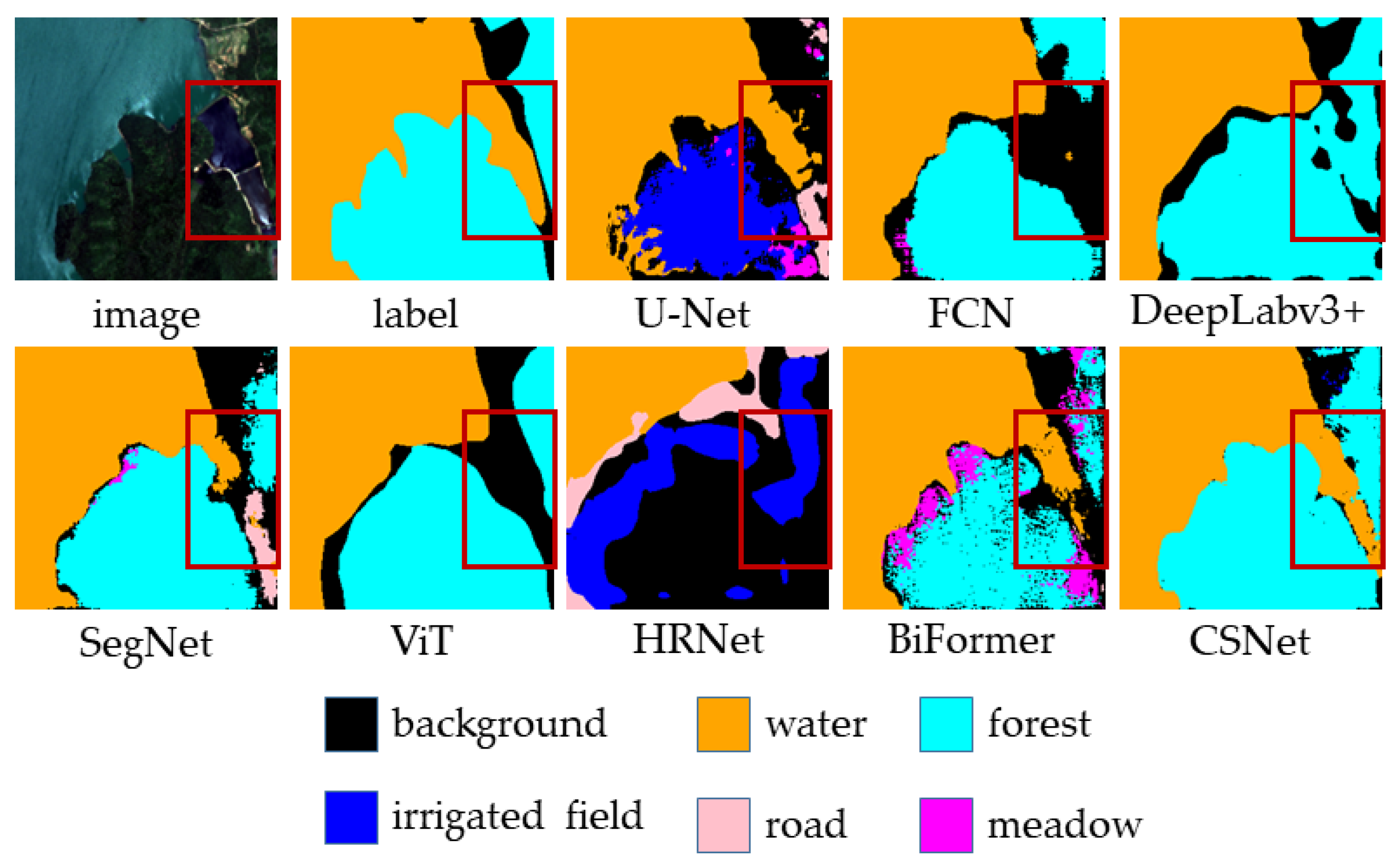
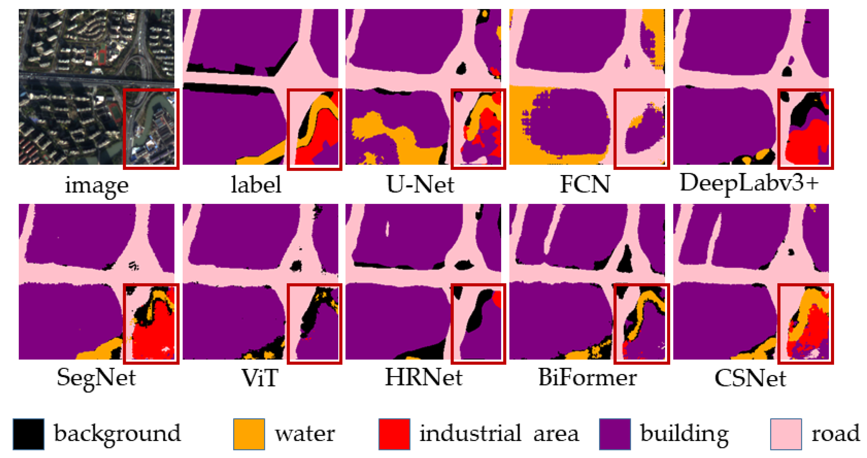
By comparing the classification results of different networks on selected samples from the test set, we further underscore the superior performance of the proposed CSNet. The visualization results indicate that CSNet not only achieves excellent classification performance across various land cover categories, but also demonstrates remarkable capability in preserving fine boundary details.

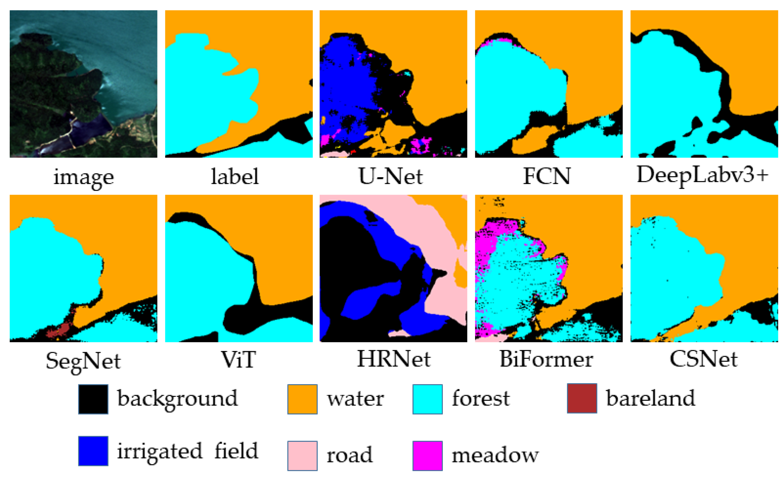
Figure 11 demonstrates the segmentation performance of different models on the water and forest categories. As seen in the figure, U-Net performs relatively well in segmenting the water category, but its segmentation ability for the forest category is poor, misclassifying most of the forest as irrigated field. FCN, DeepLabv3+, and SegNet show relatively poor segmentation performance for the water category and also struggle to accurately segment the forest category. In contrast, CSNet achieves the best segmentation results for both the water and forest categories. From a local structure perspective, there is a narrow water area on the right side of the image, which FCN, DeepLabv3+, and SegNet fail to segment. Although U-Net can segment part of it, the boundaries are blurred. This issue arises due to the skip connections present in U-Net, which help the model recover some of the structural details. CSNet, however, is able to segment this narrow water area more accurately. The combination of coordinate attention and skip connections in CSNet enables a more precise restoration of local structures in the image.

Figure 12 further demonstrates the segmentation performance of different models on local structures. In the bottom right corner of the image, there are three different land cover types: water, industrial area, and building. For this complex local structure, FCN, DeepLabv3+, and SegNet are unable to accurately segment it. U-Net can perform some segmentation of the water, but CSNet more accurately restores the location and spatial shape of all three land cover types.

The results indicate that by using skip connections, the model can fuse semantic information from different layers, helping to restore local structures. By employing the coordinate attention mechanism, CSNet can focus more on key areas of the image during feature extraction, improving the effectiveness of feature extraction and, consequently, enhancing the segmentation performance on local structures.

To further evaluate the generalization capability of the model, we conducted comparative experiments on the Vaihingen dataset. The Dice coefficient, mIoU, and overall accuracy obtained from the experiments are summarized in

Table 6. The overall performance of the comparative experiments in the Vaihingen dataset.

Model	Dice/%	mIoU/%	Overall Accuracy/%
U-Net	74.7	64.4	83.0
FCN	78.4	67.9	84.5
DeepLabV3+	80.9	69.8	84.7
SegNet	74.0	63.3	82.5
Transformer	70.4	56.6	77.7
ViT	67.9	53.5	75.5
HRNet	75.9	62.9	81.9
BiFormer	79.7	67.1	83.5
CSNet	82.7	71.2	85.3

The bolded values indicate that the network achieves the best performance on the corresponding metric.

.

It can be observed that CSNet still achieves the best performance on the Vaihingen dataset. Compared with SegNet, the Dice coefficient and mIoU are improved by 8.7% and 7.9%, respectively, while the overall accuracy increases by 2.8%.

To further validate the performance of CSNet and eliminate the influence of randomness, we conducted five experiments on the Five-Billion-Pixels dataset using CSNet and other comparative models with different random seeds. The overall accuracy for each experiment was recorded, and the results are summarized in

Table 7. Overall accuracy across multiple experiments.

	Test 1/%	Test 2/%	Test 3/%	Test 4/%	Test 5/%	Average Overall Accuracy/%
U-Net	85.1	85.6	86.0	85.7	85.5	85.6
FCN	84.0	84.3	84.5	84.2	84.1	84.2
DeepLabv3+	86.5	86.8	87.3	87.0	86.6	86.8
SegNet	83.9	84.2	84.4	84.0	84.1	84.1
Transformer	79.6	80.1	80.2	79.8	80.0	79.9
ViT	80.2	80.6	80.9	80.5	80.4	80.5
HRNet	65.9	66.3	66.5	66.2	66.0	66.2
BiFormer	88.3	88.7	88.9	88.5	88.6	88.6
CSNet	90.5	90.1	89.7	90.2	89.6	90.0

.

Based on the results of the five experiments, CSNet achieved a mean overall accuracy of 90.02% with a standard deviation of 0.36%. The 95% confidence interval was [89.58%, 90.46%]. A significance test was conducted against BiFormer, the best-performing baseline model, yielding a t-value of 7.12 and a p-value of 0.0002, indicating a statistically significant advantage of CSNet.

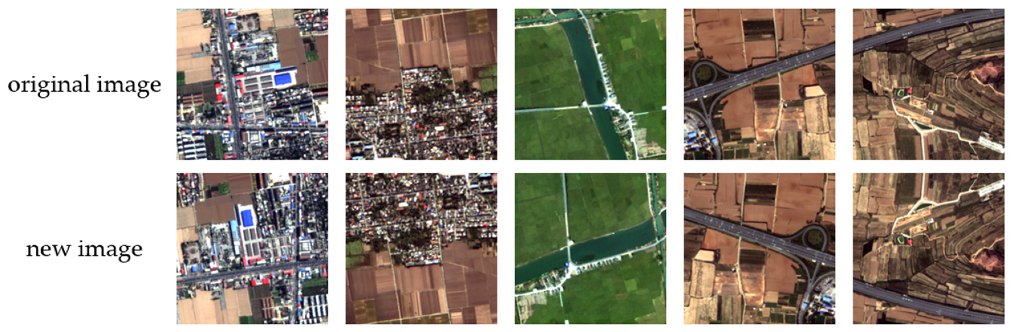
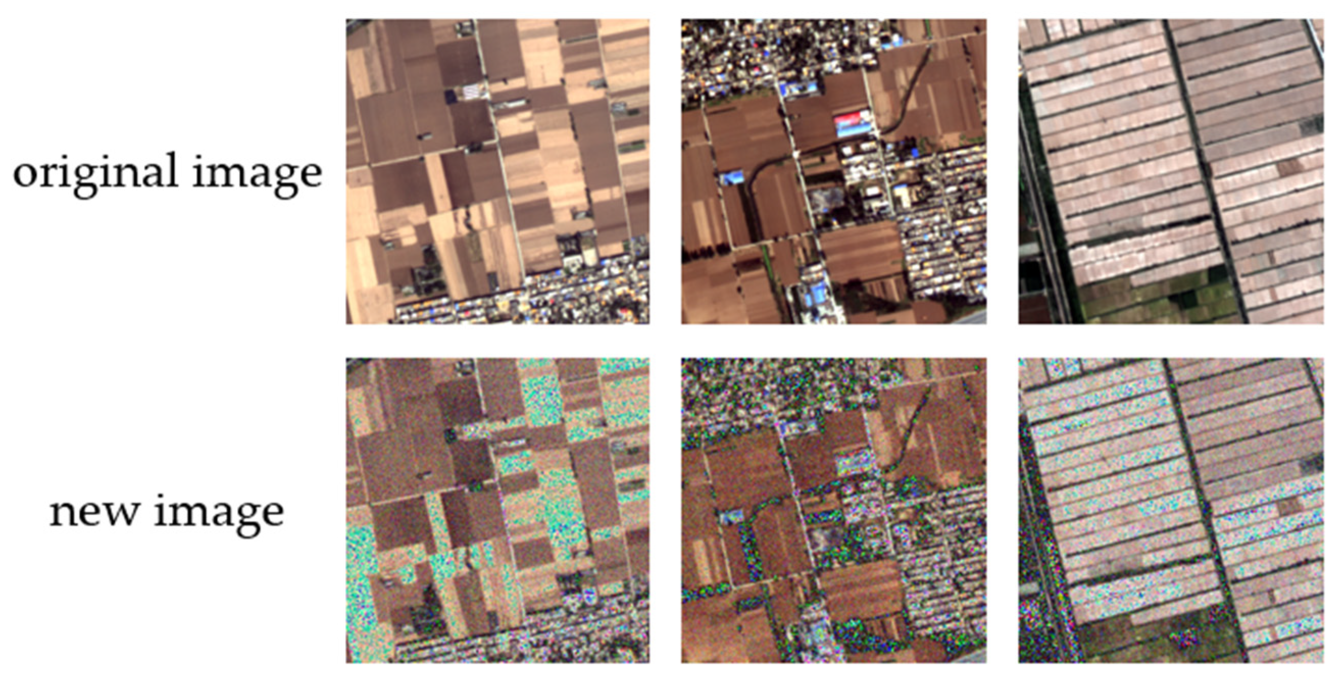
To assess the impact of geometric perturbations on CSNet, we applied small-scale translations (±10 pixels), slight rotations (±15°), and 90° rotations to the images in the Five-Billion-Pixels dataset. Comparative experiments between CSNet and other models were conducted under these conditions, and the results are presented in

Table 8. The mIoU under geometric perturbations.

	Original mIoU/%	±10 pixels/%	Drop/%	±15°/%	Drop/%	90°/%	Drop/%
U-Net	66.7	59.8	−6.9	58.2	−8.5	62.5	−4.2
FCN	61.1	54.2	−6.9	53.5	−7.6	56.8	−4.3
DeepLabv3+	66.2	60.4	−5.8	59.1	−7.1	63.6	−2.6
SegNet	63.8	57.0	−6.8	55.6	−8.2	60.7	−3.1
Transformer	50.7	43.2	−7.5	41.0	−9.7	46.1	−4.6
ViT	50.6	42.5	−8.1	39.6	−11.0	44.5	−6.1
HRNet	46.3	38.7	−7.6	36.4	−9.9	41.5	−4.8
BiFormer	68.0	63.5	−4.5	62.0	−6.0	65.0	−3.0
CSNet	70.3	67.1	−3.2	66.0	−4.3	68.4	−1.9

The bolded values indicate that the network achieves the best performance on the corresponding metric.

.

Compared with other models, CSNet exhibits the smallest variation in mIoU, indicating its superior robustness to geometric perturbations. Figure 13 presents the segmentation results of Figure 11 after a 90° rotation. As shown in the figure, even after a 90° rotation, CSNet still achieves the best segmentation performance.

3.3. Ablation Experiment

To validate the effectiveness of skip connections and coordinate attention structures in the network, as well as the impact of different positions of coordinate attention addition on the model, ablation experiments were conducted. The experiments were performed on the original SegNet network, a SegNet network with coordinate attention structure added only in the encoder (SegNet + CA), a SegNet network with skip connections only (SegNet + SC), and the CSNet network. The experimental results are shown in

Table 9. The overall performance of the ablation experiments.

Model	Dice/%	mIoU/%	Overall Accuracy/%
SegNet	76.5	63.8	84.4
SegNet + CA	79.6	68.0	88.9
SegNet + SC	77.4	64.9	86.6
CSNet	81.4	70.3	90.5

The bolded values indicate that the network achieves the best performance on the corresponding metric.

.

After adding the coordinate attention mechanism, the model’s Dice coefficient and mIoU increased by 3.1% and 4.2%, respectively, indicating that the model’s segmentation capability for small targets and small sample categories has improved. The overall accuracy (OA) increased by 4.5%, demonstrating that the model’s ability to segment the entire dataset has been enhanced. After adding skip connections, the model’s Dice coefficient and mIoU showed slight improvements, suggesting that the fusion of semantic information from different layers helps restore the spatial information of the image and improves the segmentation capability for small targets. OA increased by 2.2%, indicating an overall enhancement in the model’s segmentation ability. Compared to SegNet, CSNet achieved increases of 4.9%, 6.5%, and 6.1% in Dice coefficient, mIoU, and OA, respectively, demonstrating the model’s strong segmentation capability for various target categories.

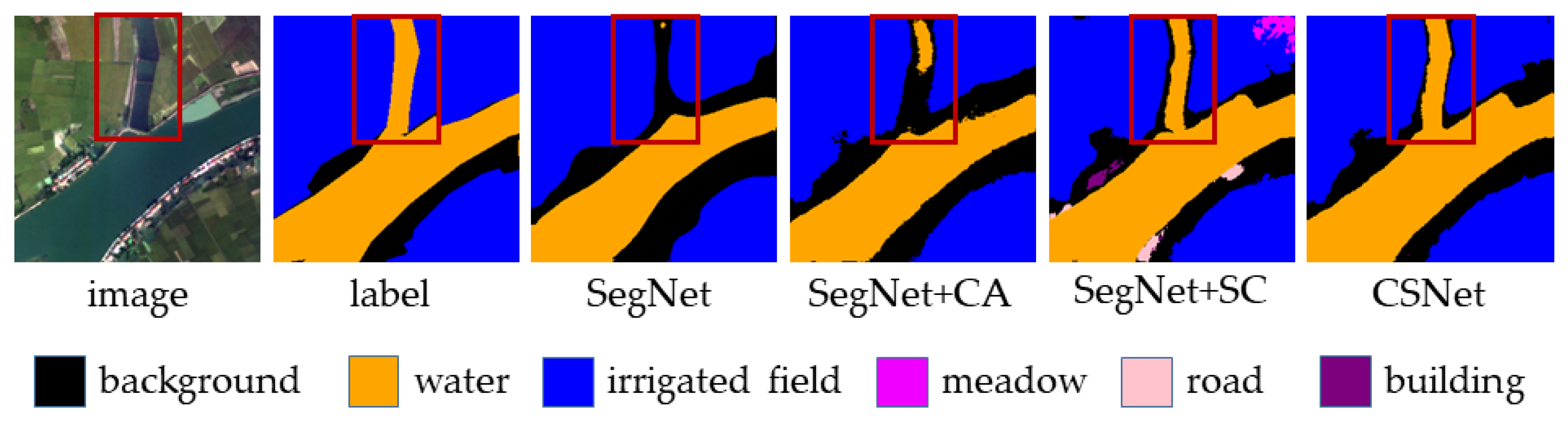
Figure 14 illustrates the segmentation results of different networks for the water and irrigated field classes in the ablation study. It can be observed that after adding skip connections, the model is able to segment the slender river structures, indicating that skip connections help restore the shape information of geographic features. However, the results with skip connections also show some instances of misclassification. Upon incorporating coordinate attention, the model eliminates these misclassifications and successfully segments water regions that SegNet failed to detect. Additionally, the segmentation of irrigated fields becomes more accurate, demonstrating that coordinate attention enhances the model’s ability to distinguish between different land cover types.

Figure 15 presents the segmentation results for paddy field and irrigated field in the ablation study across different network variants. Due to the spectral similarity between paddy field and irrigated field, SegNet misclassifies part of the paddy field as water. After incorporating skip connections, the boundary ambiguity is alleviated; however, the extent of misclassification becomes more severe. With the introduction of coordinate attention, the misclassification is significantly reduced, with almost no confusion observed. This indicates that the coordinate attention mechanism helps the model better distinguish between spectrally similar land cover types.

4. Discussion

For certain categories in the Five-Billion-Pixels dataset, such as meadow, CSNet achieves a Precision of only 61.6% and an IoU of 35.1%, indicating that the segmentation performance remains suboptimal. To enhance CSNet’s effectiveness on the meadow class, further improvements to the network could be considered based on the specific characteristics of this category.

In addition, while the Precision scores for the industrial area and road categories are relatively high, their IoU values are only 58.3% and 51.6%, respectively. For the industrial area category, misclassification with the building class and the complexity of boundary shapes pose challenges to accurate segmentation. For the road category, the narrow width of the objects makes it difficult for CSNet to accurately capture their shapes. To address these issues, augmenting the network architecture to improve its ability to delineate object boundaries may be a promising direction.

5. Conclusions

In this study, we propose CSNet, an improved architecture based on SegNet, to address the limitations of the SegNet network in remote sensing image segmentation. The proposed network builds upon SegNet by incorporating coordinate attention and skip connections, as well as optimizing the loss function. In the encoder section, the coordinate attention mechanism is applied to the output of each encoder layer to enhance features, enabling the model to focus more on global information and improving its ability to extract detailed features. Skip connections are inserted between the encoder and decoder, directly linking the encoder with the corresponding decoder, transferring shallow features to the decoder. This not only helps preserve important spatial details but also strengthens the gradient flow across the network, mitigating the vanishing gradient problem and accelerating the training process, thereby enhancing training efficiency. Additionally, using a combination of weighted cross-entropy loss and Dice coefficient loss, alongside merging some categories in the dataset, effectively addresses the class imbalance issue and improves segmentation accuracy for underrepresented categories.

Compared to U-Net, FCN, DeepLabv3+, and SegNet networks, CSNet outperforms them, with the best Dice coefficient, mIoU, and overall accuracy of 81.4%, 70.3%, and 90.5%, respectively. Moreover, from the segmentation results, CSNet shows superior performance in handling local structures and land cover boundaries. The results indicate that CSNet can achieve semantic segmentation for multi-class remote sensing images, offering improved segmentation accuracy and better handling of local structures and land cover boundaries compared to other networks.

References

1. Kussul, N.; Lavreniuk, M.; Skakun, S.; Shelestov, A. Deep Learning Classification of Land Cover and Crop Types Using Remote Sensing Data. IEEE Geosci. Remote Sens. Lett. 2017, 14, 778–782. [Google Scholar] [CrossRef]
2. Tong, X.-Y.; Xia, G.-S.; Lu, Q.; Shen, H.; Li, S.; You, S.; Zhang, L. Land-Cover Classification with High-Resolution Remote Sensing Images Using Transferable Deep Models. Remote Sens. Environ. 2020, 237, 111322. [Google Scholar] [CrossRef]
3. Shao, Z.; Tang, P.; Wang, Z.; Saleem, N.; Yam, S.; Sommai, C. BRRNet: A Fully Convolutional Neural Network for Automatic Building Extraction from High-Resolution Remote Sensing Images. Remote Sens. 2020, 12, 1050. [Google Scholar] [CrossRef]
4. Vakalopoulou, M.; Karantzalos, K.; Komodakis, N.; Paragios, N. Building Detection in Very High Resolution Multispectral Data with Deep Learning Features. In Proceedings of the 2015 IEEE International Geoscience and Remote Sensing Symposium (IGARSS), Milan, Italy, 26–31 July 2015; IEEE: Piscataway, NJ, USA, 2015; pp. 1873–1876. [Google Scholar]
5. Cao, R.; Tu, W.; Yang, C.; Li, Q.; Liu, J.; Zhu, J.; Zhang, Q.; Li, Q.; Qiu, G. Deep Learning-Based Remote and Social Sensing Data Fusion for Urban Region Function Recognition. ISPRS J. Photogramm. Remote Sens. 2020, 163, 82–97. [Google Scholar] [CrossRef]
6. Wang, D.; Liu, S.; Zhang, C.; Xu, M.; Yang, J.; Yasir, M.; Wan, J. An Improved Semantic Segmentation Model Based on SVM for Marine Oil Spill Detection Using SAR Image. Mar. Pollut. Bull. 2023, 192, 114981. [Google Scholar] [CrossRef]
7. Himeur, Y.; Rimal, B.; Tiwary, A.; Amira, A. Using Artificial Intelligence and Data Fusion for Environmental Monitoring: A Review and Future Perspectives. Inf. Fusion 2022, 86–87, 44–75. [Google Scholar] [CrossRef]
8. Khan, S.D.; Basalamah, S. Multi-Scale and Context-Aware Framework for Flood Segmentation in Post-Disaster High Resolution Aerial Images. Remote Sens. 2023, 15, 2208. [Google Scholar] [CrossRef]
9. Melgani, F.; Bruzzone, L. Classification of Hyperspectral Remote Sensing Images with Support Vector Machines. IEEE Trans. Geosci. Remote Sens. 2004, 42, 1778–1790. [Google Scholar] [CrossRef]
10. Fauvel, M.; Benediktsson, J.; Chanussot, J.; Sveinsson, J. Spectral and Spatial Classification of Hyperspectral Data Using SVMs and Morphological Profiles. IEEE Trans. Geosci. Remote Sens. 2008, 46, 3804–3814. [Google Scholar] [CrossRef]
11. Gislason, P.O.; Benediktsson, J.A.; Sveinsson, J.R. Random Forests for Land Cover Classification. Pattern Recognit. Lett. 2006, 27, 294–300. [Google Scholar] [CrossRef]
12. Pal, M. Random Forest Classifier for Remote Sensing Classification. Int. J. Remote Sens. 2005, 26, 217–222. [Google Scholar] [CrossRef]
13. Krizhevsky, A.; Sutskever, I.; Hinton, G.E. ImageNet Classification with Deep Convolutional Neural Networks. Commun. ACM 2017, 60, 84–90. [Google Scholar] [CrossRef]
14. Long, J.; Shelhamer, E.; Darrell, T. Fully Convolutional Networks for Semantic Segmentation. In Proceedings of the 2015 IEEE Conference on Computer Vision and Pattern Recognition (CVPR), Boston, MA, USA, 7–12 June 2015; IEEE: Piscataway, NJ, USA, 2015; pp. 3431–3440. [Google Scholar]
15. Ronneberger, O.; Fischer, P.; Brox, T. U-Net: Convolutional Networks for Biomedical Image Segmentation. In Medical Image Computing and Computer-Assisted Intervention—MICCAI 2015; Navab, N., Hornegger, J., Wells, W.M., Frangi, A.F., Eds.; Lecture Notes in Computer Science; Springer International Publishing: Cham, Switzerland, 2015; Volume 9351, pp. 234–241. ISBN 978-3-319-24573-7. [Google Scholar]
16. Chen, G.; Zhang, X.; Wang, Q.; Dai, F.; Gong, Y.; Zhu, K. Symmetrical Dense-Shortcut Deep Fully Convolutional Networks for Semantic Segmentation of Very-High-Resolution Remote Sensing Images. IEEE J. Sel. Top. Appl. Earth Obs. Remote Sens. 2018, 11, 1633–1644. [Google Scholar] [CrossRef]
17. Chen, L.-C.; Zhu, Y.; Papandreou, G.; Schroff, F.; Adam, H. Encoder-Decoder with Atrous Separable Convolution for Semantic Image Segmentation. In Computer Vision—ECCV 2018; Ferrari, V., Hebert, M., Sminchisescu, C., Weiss, Y., Eds.; Lecture Notes in Computer Science; Springer International Publishing: Cham, Switzerland, 2018; Volume 11211, pp. 833–851. ISBN 978-3-030-01233-5. [Google Scholar]
18. Sun, K.; Zhao, Y.; Jiang, B.; Cheng, T.; Xiao, B.; Liu, D.; Mu, Y.; Wang, X.; Liu, W.; Wang, J. High-Resolution Representations for Labeling Pixels and Regions. arXiv 2019, arXiv:1904.04514. [Google Scholar]
19. Zhang, Y.; Wang, L.; Yang, R.; Chen, N.; Zhao, Y.; Dai, Q. Semantic Segmentation of High Spatial Resolution Remote Sensing Imagery Based on Weighted Attention U-Net. In Proceedings of the Fourteenth International Conference on Graphics and Image Processing (ICGIP 2022), Nanjing, China, 27 June 2023; Xiao, L., Xue, J., Eds.; SPIE: Bellingham, WA, USA, 2023; p. 107. [Google Scholar]
20. Yi, Y.; Zhang, Z.; Zhang, W.; Zhang, C.; Li, W.; Zhao, T. Semantic Segmentation of Urban Buildings from VHR Remote Sensing Imagery Using a Deep Convolutional Neural Network. Remote Sens. 2019, 11, 1774. [Google Scholar] [CrossRef]
21. Zhan, Z.; Zhang, X.; Liu, Y.; Sun, X.; Pang, C.; Zhao, C. Vegetation Land Use/Land Cover Extraction from High-Resolution Satellite Images Based on Adaptive Context Inference. IEEE Access 2020, 8, 21036–21051. [Google Scholar] [CrossRef]
22. Yu, Z.; Wan, F.; Lei, G.; Xiong, Y.; Xu, L.; Ye, Z.; Liu, W.; Zhou, W.; Xu, C. RSLC-Deeplab: A Ground Object Classification Method for High-Resolution Remote Sensing Images. Electronics 2023, 12, 3653. [Google Scholar] [CrossRef]
23. Weng, L.; Xu, Y.; Xia, M.; Zhang, Y.; Liu, J.; Xu, Y. Water Areas Segmentation from Remote Sensing Images Using a Separable Residual SegNet Network. IJGI 2020, 9, 256. [Google Scholar] [CrossRef]
24. Wu, S.; Huang, X.; Zhang, J. Application and Research of the Image Segmentation Algorithm in Remote Sensing Image Buildings. Sci. Program. 2022, 2022, 1–9. [Google Scholar] [CrossRef]
25. Narayanan, V.; Sikha, O.; Benitez, R. IARS SegNet: Interpretable Attention Residual Skip Connection SegNet for Melanoma Segmentation. IEEE ACCESS 2024, 12, 126122–126134. [Google Scholar] [CrossRef]
26. He, F.; Wang, W.; Ren, L.; Zhao, Y.; Liu, Z.; Zhu, Y. CA-SegNet: A Channel-Attention Encoder-Decoder Network for Histopathological Image Segmentation. Biomed. Signal Process. Control. 2024, 96, 106590. [Google Scholar] [CrossRef]
27. Huo, Y.; Gang, S.; Dong, L.; Guan, C. An Efficient Semantic Segmentation Method for Remote-Sensing Imagery Using Improved Coordinate Attention. Appl. Sci. 2024, 14, 4075. [Google Scholar] [CrossRef]
28. Vaswani, A.; Shazeer, N.; Parmar, N.; Uszkoreit, J.; Jones, L.; Gomez, A.N.; Kaiser, Ł.; Polosukhin, I. Attention Is All You Need. arXiv 2017, arXiv:1706.03762. [Google Scholar]
29. Dosovitskiy, A.; Beyer, L.; Kolesnikov, A.; Weissenborn, D.; Zhai, X.; Unterthiner, T.; Dehghani, M.; Minderer, M.; Heigold, G.; Gelly, S.; et al. An Image Is Worth 16 × 16 Words: Transformers for Image Recognition at Scale. In Proceedings of the 9th International Conference on Learning Representations (ICLR), Vienna, Austria, 3–7 May 2021. [Google Scholar]
30. Liu, Z.; Lin, Y.; Cao, Y.; Hu, H.; Wei, Y.; Zhang, Z.; Lin, S.; Guo, B. Swin Transformer: Hierarchical Vision Transformer Using Shifted Windows. In Proceedings of the 2021 IEEE/CVF International Conference on Computer Vision (ICCV), Montreal, QC, Canada, 10–17 October 2021; IEEE: Piscataway, NJ, USA, 2021; pp. 9992–10002. [Google Scholar]
31. Zhu, L.; Wang, X.; Ke, Z.; Zhang, W.; Lau, R. BiFormer: Vision Transformer with Bi-Level Routing Attention. In Proceedings of the 2023 IEEE/CVF Conference on Computer Vision and Pattern Recognition (CVPR), Vancouver, BC, Canada, 17 June 2023; pp. 10323–10333. [Google Scholar]
32. Chen, Q.; Yan, Y.; Wang, X.; Peng, J. IMViT: Adjacency Matrix-Based Lightweight Plain Vision Transformer. IEEE ACCESS 2025, 13, 18535–18545. [Google Scholar] [CrossRef]
33. Cheng, J.; Deng, C.; Su, Y.; An, Z.; Wang, Q. Methods and Datasets on Semantic Segmentation for Unmanned Aerial Vehicle Remote Sensing Images: A Review. ISPRS J. Photogramm. Remote Sens. 2024, 211, 1–34. [Google Scholar] [CrossRef]
34. Bai, Y.; Mas, E.; Koshimura, S. Towards Operational Satellite-Based Damage-Mapping Using U-Net Convolutional Network: A Case Study of 2011 Tohoku Earthquake-Tsunami. Remote Sens. 2018, 10, 1626. [Google Scholar] [CrossRef]
35. Badrinarayanan, V.; Kendall, A.; Cipolla, R. SegNet: A Deep Convolutional Encoder-Decoder Architecture for Image Segmentation. IEEE Trans. Pattern Anal. Mach. Intell. 2017, 39, 2481–2495. [Google Scholar] [CrossRef]
36. Hou, Q.; Zhou, D.; Feng, J. Coordinate Attention for Efficient Mobile Network Design. In Proceedings of the 2021 IEEE/CVF Conference on Computer Vision and Pattern Recognition (CVPR), Nashville, TN, USA, 19–25 June 2021; IEEE: Piscataway, NJ, USA, 2021; pp. 13708–13717. [Google Scholar]
37. Ben Naceur, M.; Akil, M.; Saouli, R.; Kachouri, R. Fully Automatic Brain Tumor Segmentation with Deep Learning-Based Selective Attention Using Overlapping Patches and Multi-Class Weighted Cross-Entropy. Med. Image Anal. 2020, 63, 101692. [Google Scholar] [CrossRef]
38. Chen, D.; Lu, Y.; Li, Z.; Young, S. Performance Evaluation of Deep Transfer Learning on Multi-Class Identification of Common Weed Species in Cotton Production Systems. Comput. Electron. Agric. 2022, 198, 107091. [Google Scholar] [CrossRef]
39. Fan, Z.; Hou, J.; Zang, Q.; Chen, Y.; Yan, F. River Segmentation of Remote Sensing Images Based on Composite Attention Network. Complexity 2022, 2022, 7750281. [Google Scholar] [CrossRef]
40. Kang, D.; Park, S.; Paik, J. SdBAN: Salient Object Detection Using Bilateral Attention Network with Dice Coefficient Loss. IEEE Access 2020, 8, 104357–104370. [Google Scholar] [CrossRef]
41. Tong, X.Y.; Xia, G.-S.; Zhu, X.X. Enabling Country-Scale Land Cover Mapping with Meter-Resolution Satellite Imagery. ISPRS J. Photogramm. Remote Sens. 2023, 196, 178–196. [Google Scholar] [CrossRef]
Figure 1. The network architecture of SegNet [35].
Remotesensing 17 02048 g001
Figure 2. The network architecture of CSNet.
Remotesensing 17 02048 g002
Figure 3. The structure diagram of the coordinate attention [36].
Remotesensing 17 02048 g003
Figure 4. The pixel counts for each class in the dataset.
Remotesensing 17 02048 g004
Figure 5. The pixel counts of each class after merging the categories.
Remotesensing 17 02048 g005
Figure 6. Images in the dataset with an excessive proportion of background pixels.
Remotesensing 17 02048 g006
Figure 7. The proportion of background pixels in the dataset.
Remotesensing 17 02048 g007
Figure 8. Performing rotation and flipping operations on the images in the dataset.
Remotesensing 17 02048 g008
Figure 9. Performing brightness enhancement on the images in the dataset.
Remotesensing 17 02048 g009
Figure 10. Adding Gaussian noise to the images in the dataset.
Remotesensing 17 02048 g010
Figure 11. Segmentation results of different models on water and forest. The red frame highlights the key region.
Remotesensing 17 02048 g011
Figure 12. Segmentation performance of different models on local structures. The red frames highlight the key regions.
Remotesensing 17 02048 g012
Figure 13. Comparison of segmentation results after 90° rotation.
Remotesensing 17 02048 g013
Figure 14. Partial water segmentation results from the ablation study. The red frames highlight the key regions.
Remotesensing 17 02048 g014
Figure 15. Partial segmentation results of paddy field and irrigated field from the ablation study.
Remotesensing 17 02048 g015