
High-Resolution Wide-Beam Millimeter-Wave ArcSAR System for Urban Infrastructure Monitoring


Abstract
1. Introduction
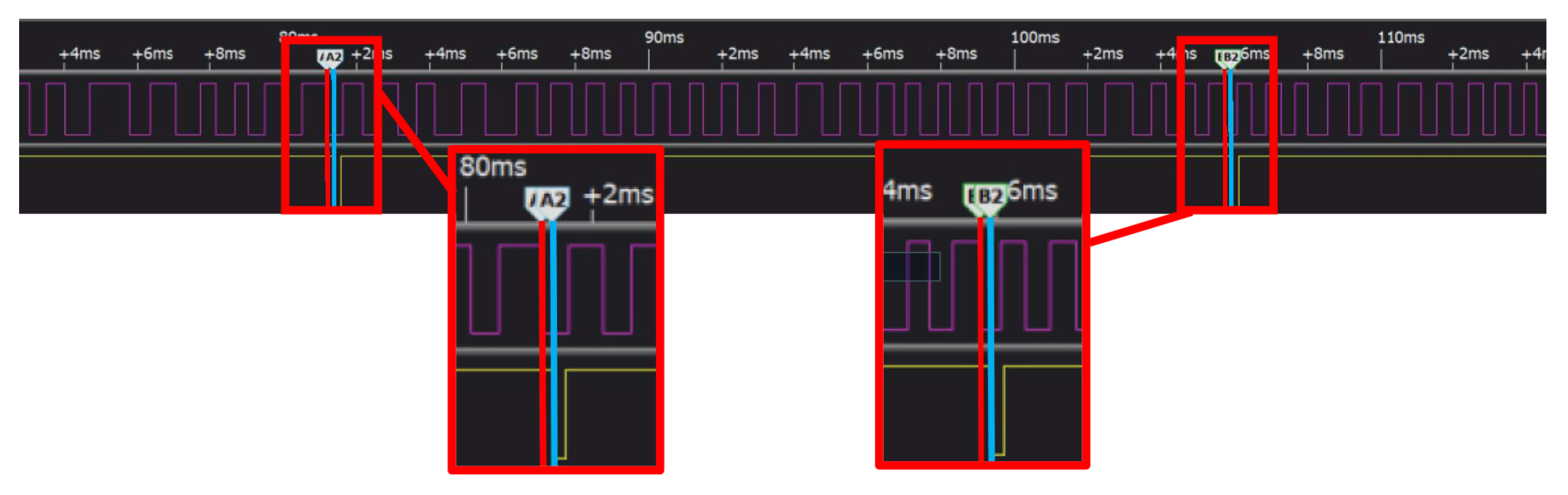
- First, in this study, a mmwave ArcSAR system is proposed, and it uses the TI 6843 module as a radar sensor. To handle the non-uniform azimuth sampling caused by motor motion, a high-accuracy angular coder is used in the system design. The coder can send the radar a hardware trigger signal to indicate when to rotate to a specific angle so that uniform angular sampling can be achieved under the unstable rotation of the motor. The time delay of the hardware trigger signal and its influence on focusing are analyzed.
- Second, the ArcSAR’s maximum azimuth sampling angle that can avoid aliasing is deducted based on the Nyquist theorem. The mathematical relation supports the proposed ArcSAR system in acquiring data by setting the sampling angle interval. The relation is validated via simulations and real data experiments.
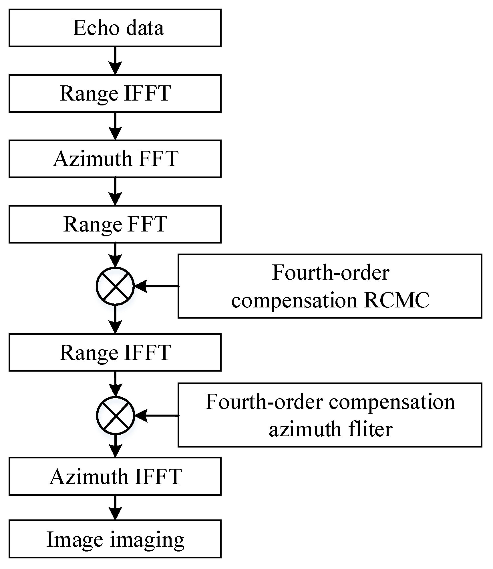
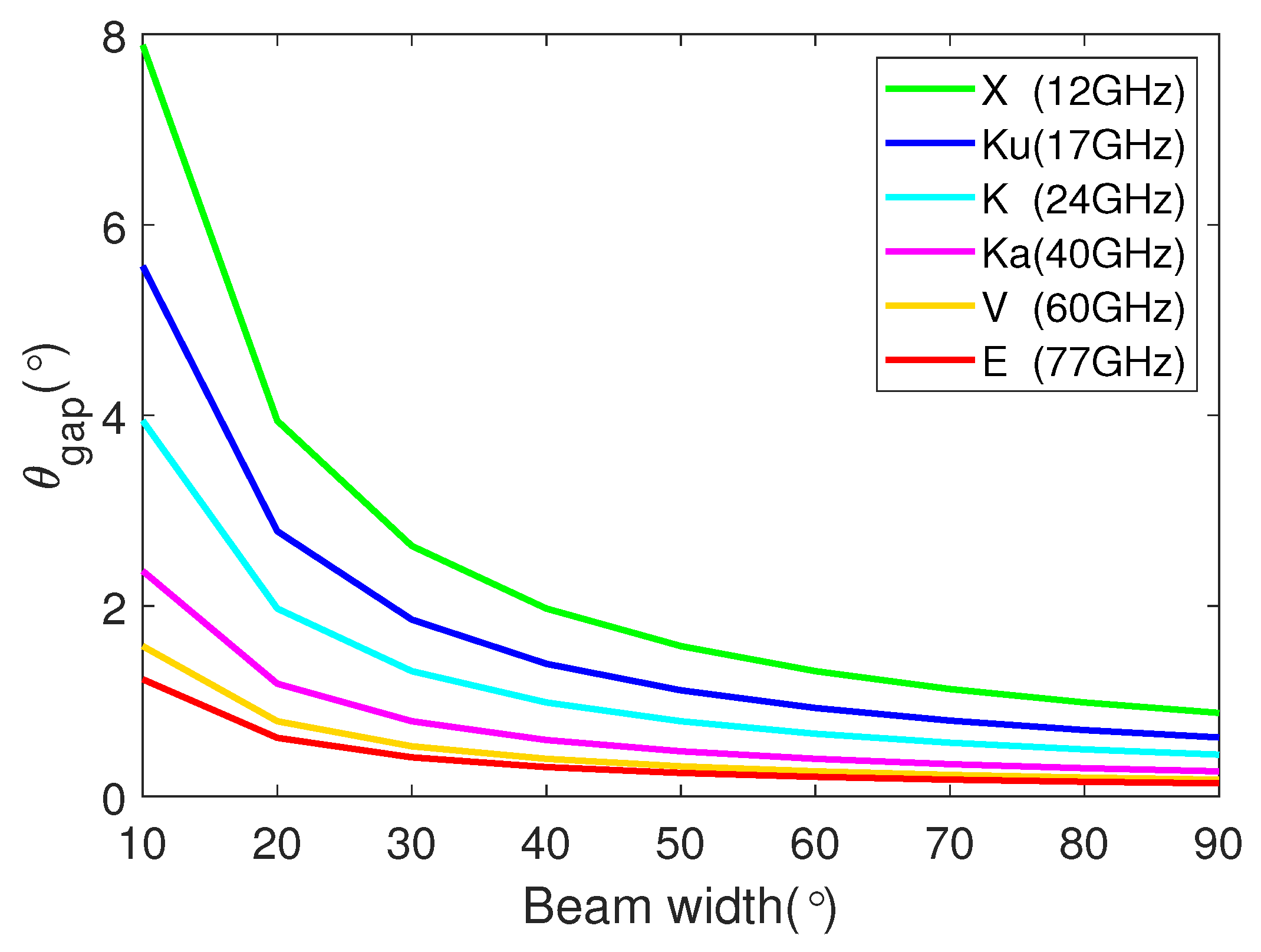
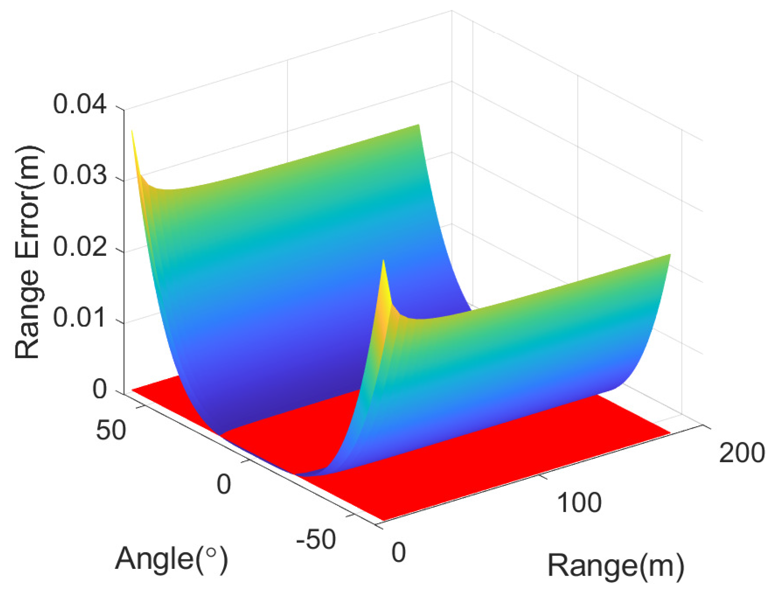
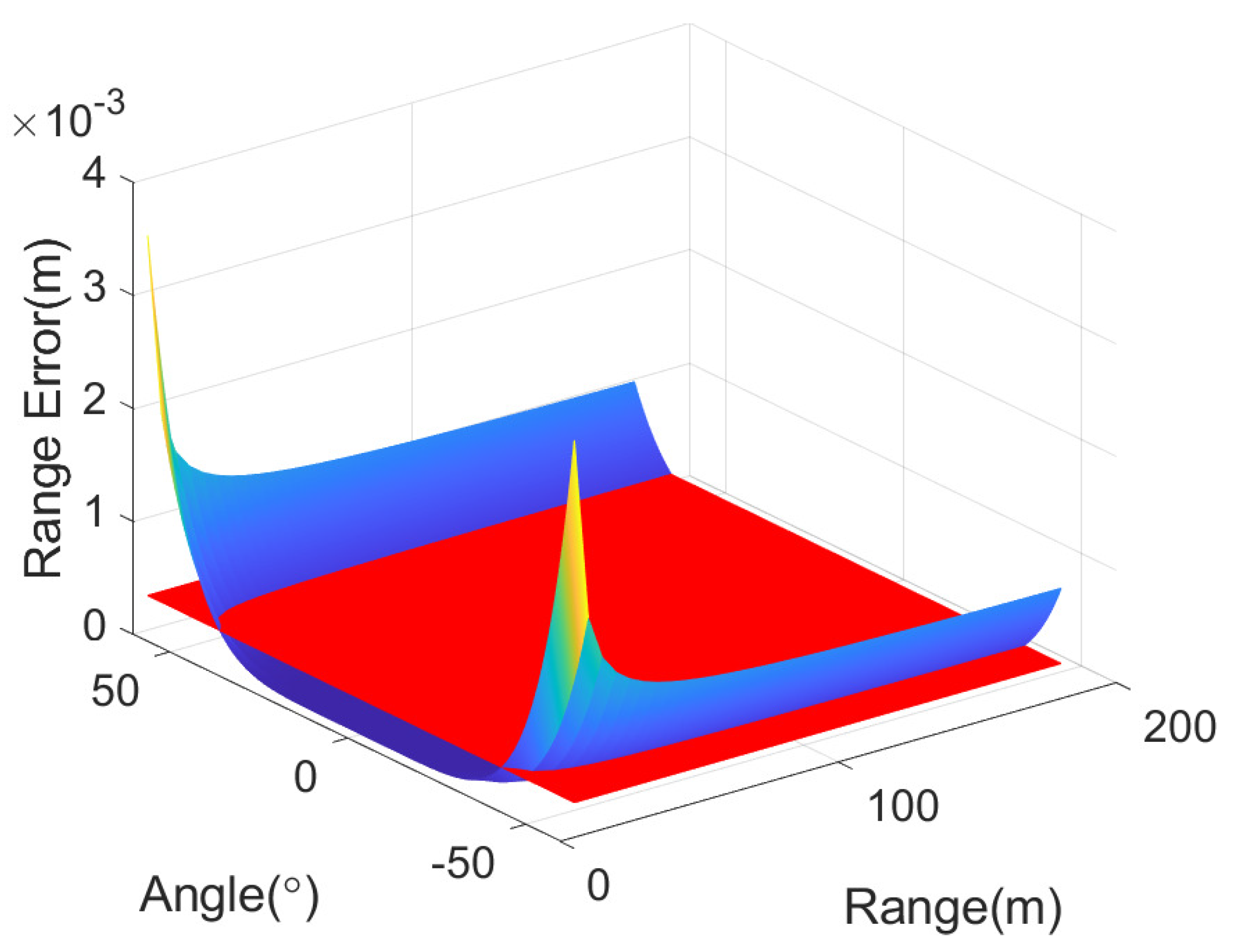
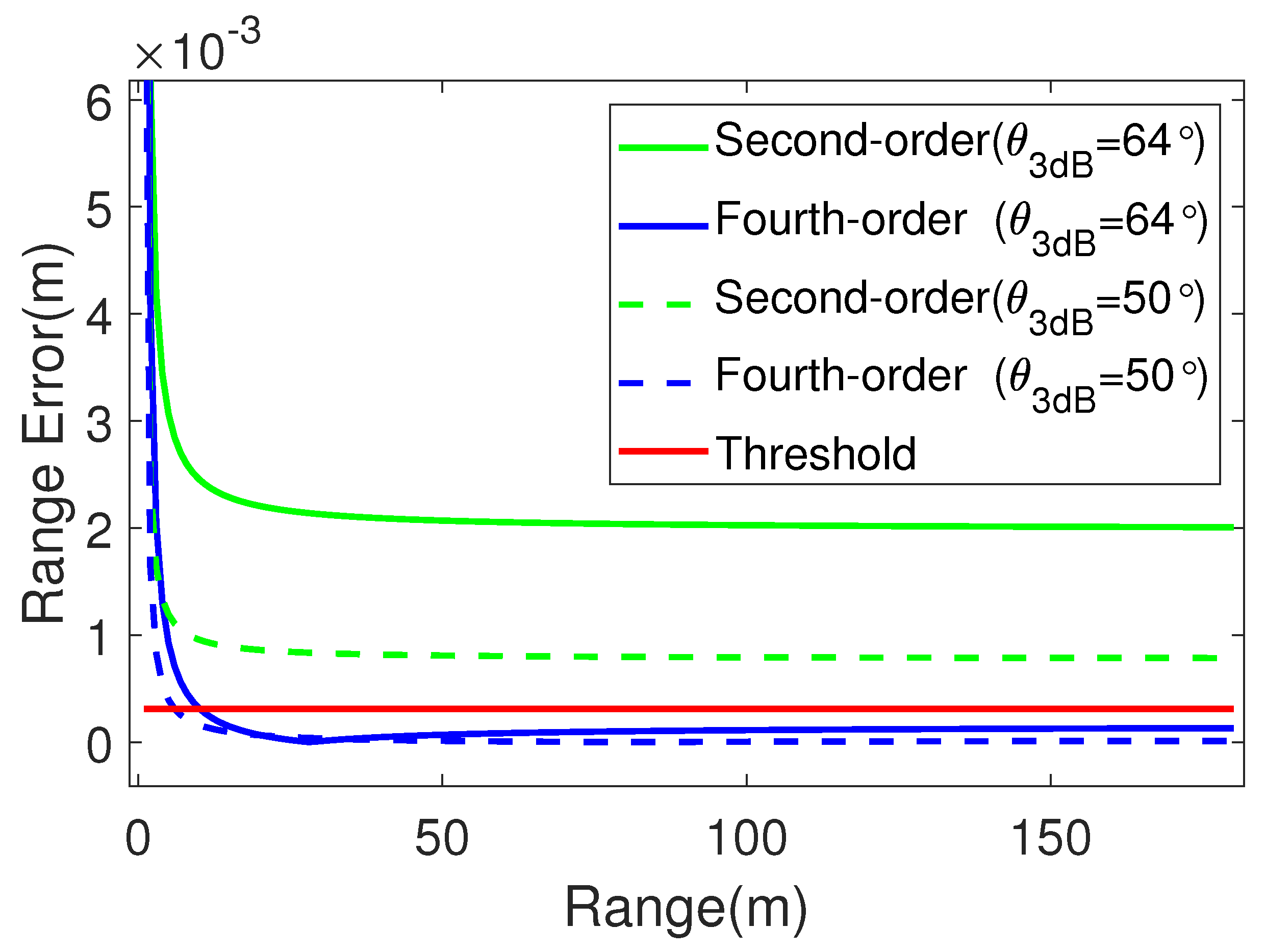
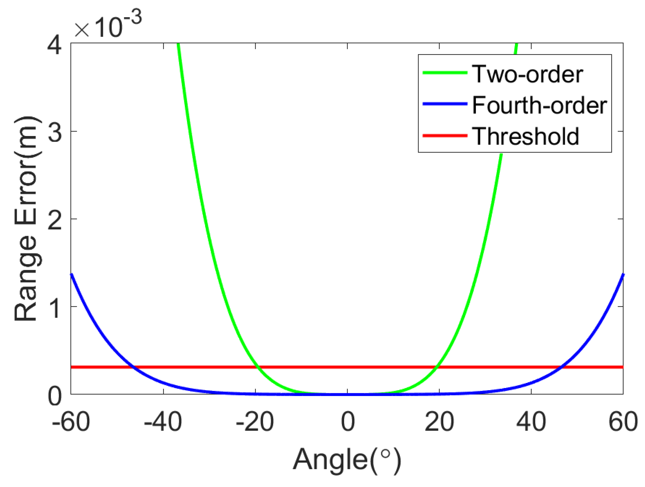
- Third, the range cell migration (RCM) phenomenon is severe because mmwave radar has a wide azimuth beamwidth and a high frequency, and ArcSAR has a curved synthetic aperture. The second-order approximation based on Taylor expansion is typically used for modeling. One viable solution is increasing the approximation order. Considering that the odd-order term in Taylor expansion is zero when in side-looking mode, the first- and third-order terms do not exist. Therefore, a forth-order expansion approximation formula for RCM would be enough in most cases, and this is shown in the following section. Hence, the fourth-order RCM model based on the range-Doppler (RD) algorithm is interpreted with a uniform azimuth angle to suit the system and implemented. The focusing performance of the imaging algorithm is thoroughly analyzed and validated using both simulation and real data.
2. Method
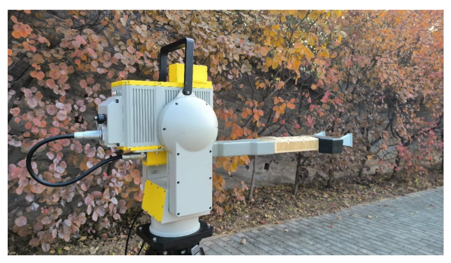
2.1. Design of the ArcSAR System
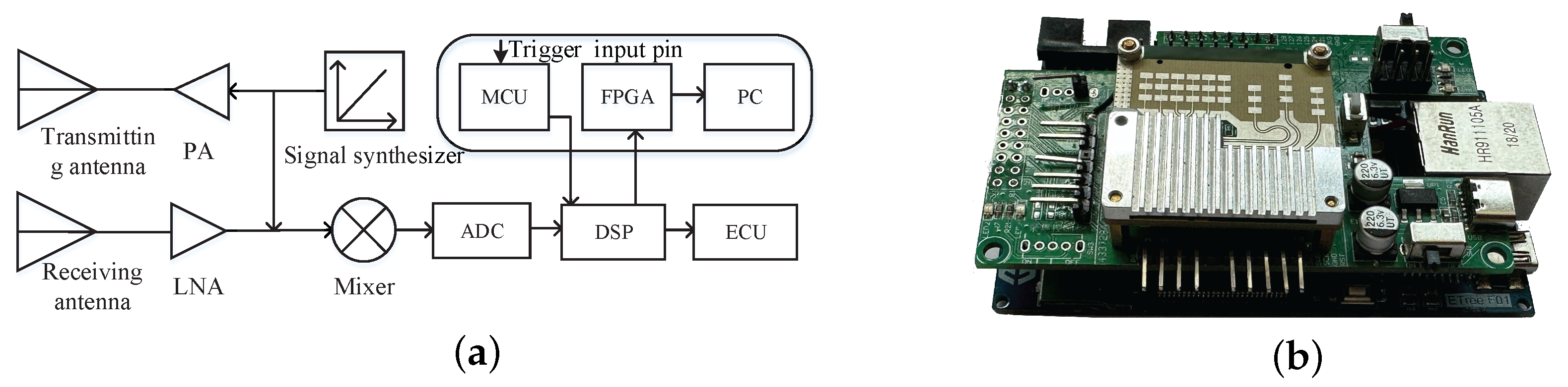
2.1.1. Mmwave Radar Module
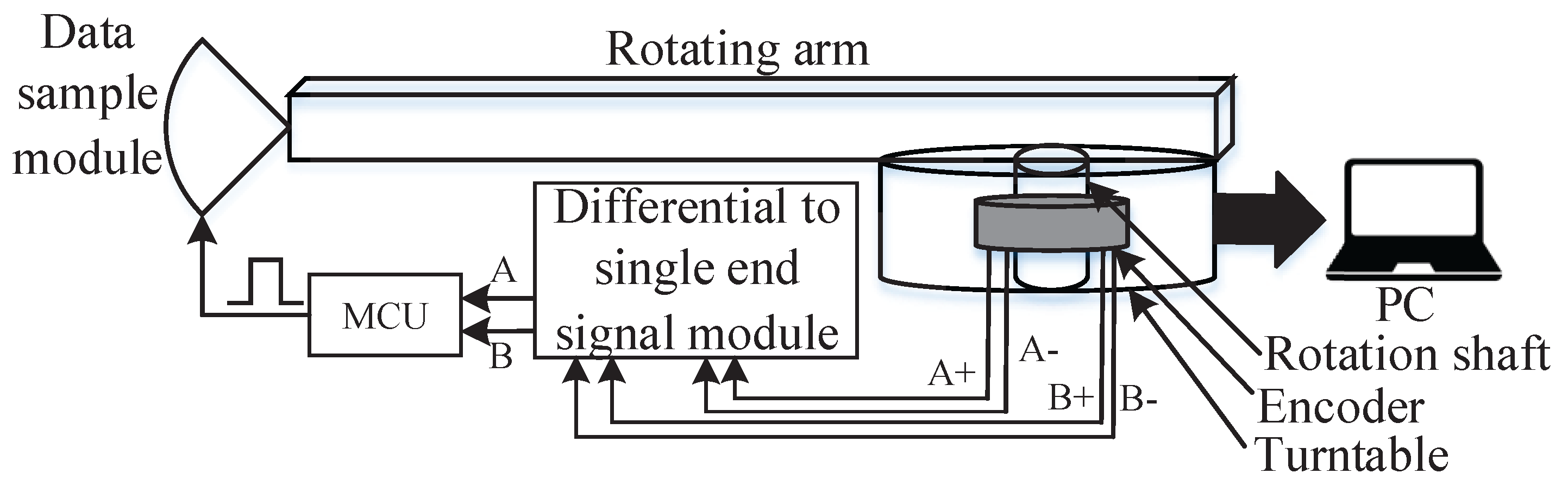
2.1.2. Motion Platform Module
2.1.3. Power Supply Module
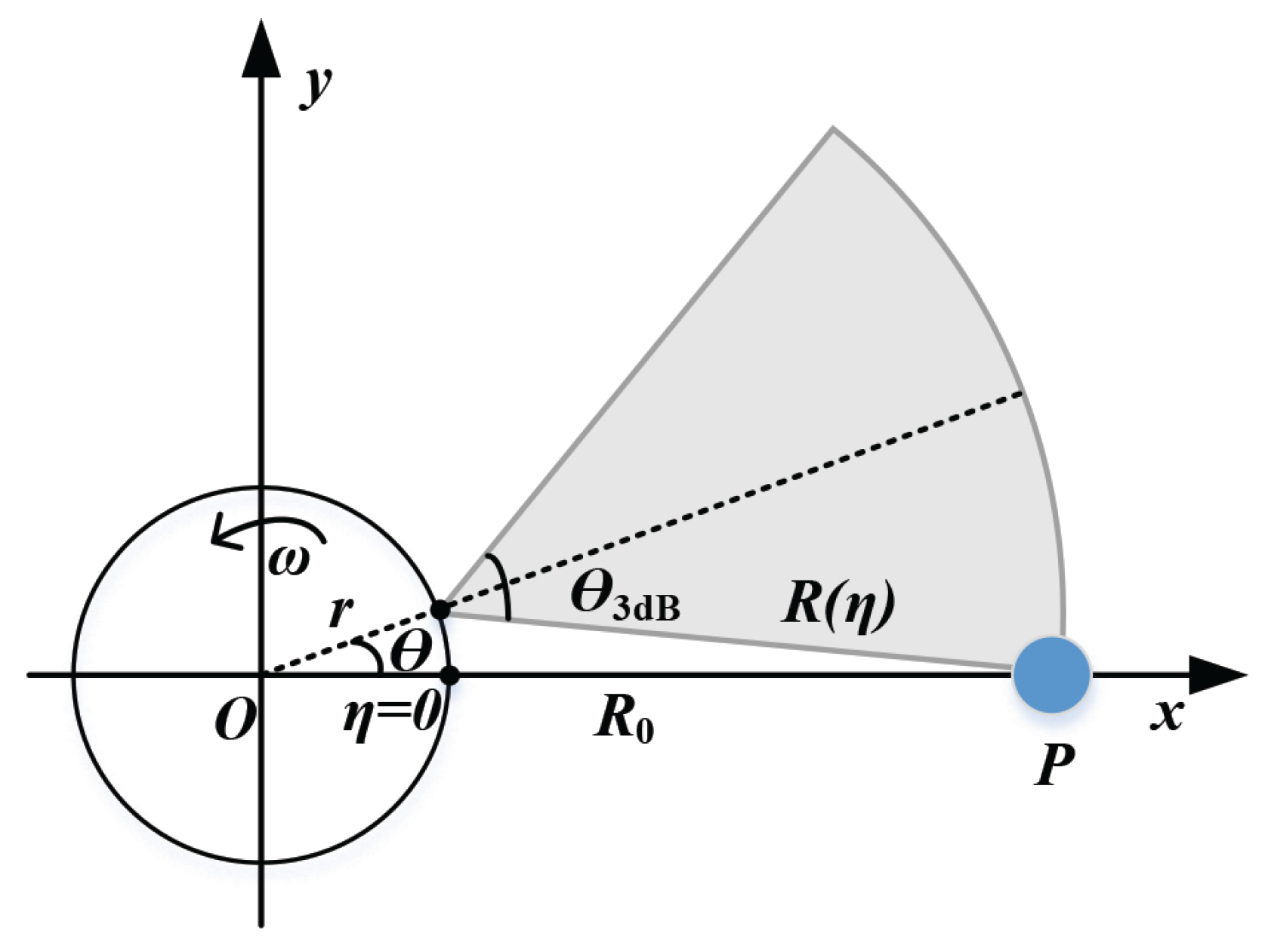
2.2. Signal Model
2.3. Fourth-Order RD Algorithm
2.4. System Performance Analysis
2.4.1. Maximum Angular Sampling Interval
2.4.2. Imaging Error Analysis Based on Order of Range Equation
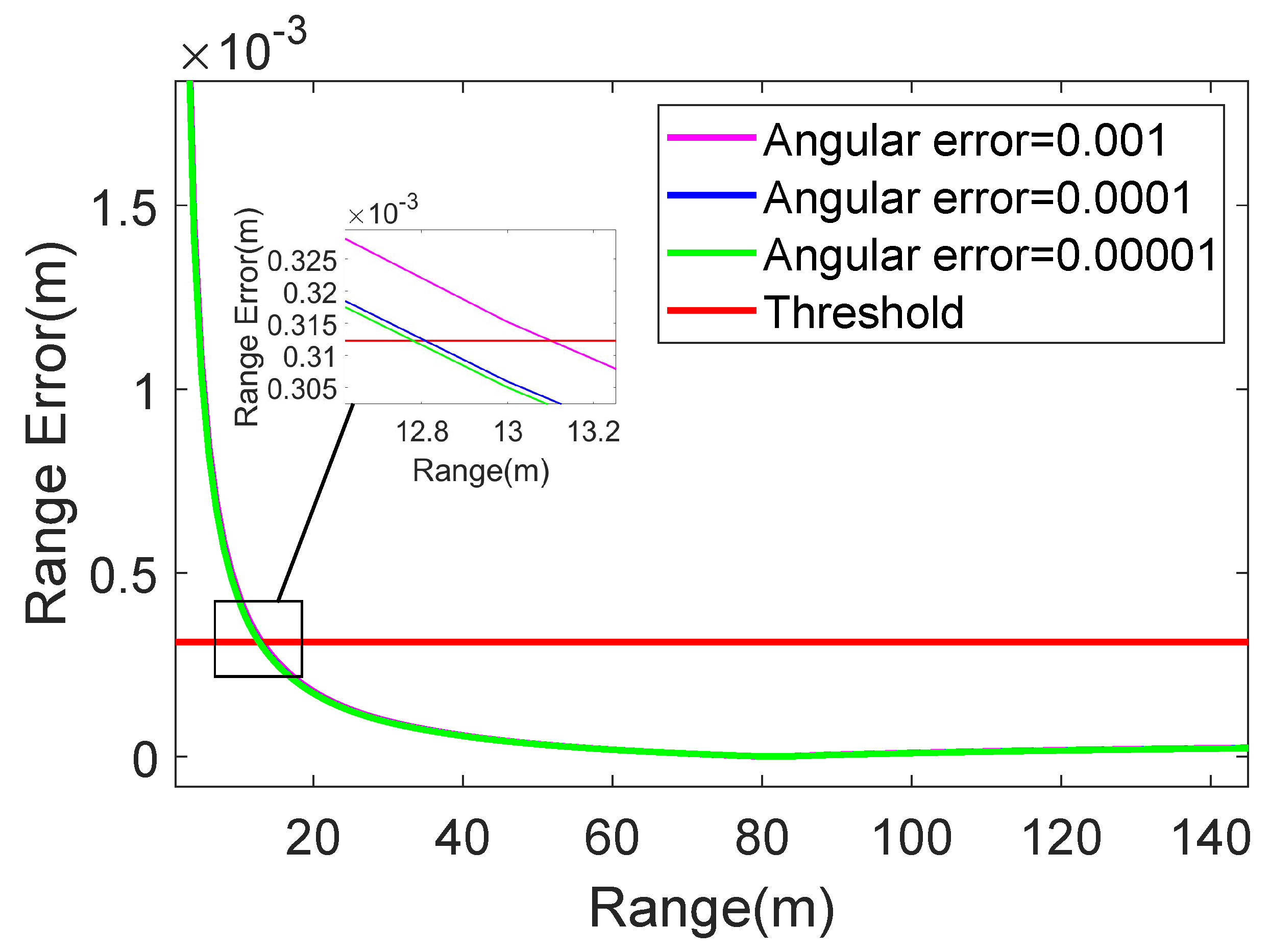
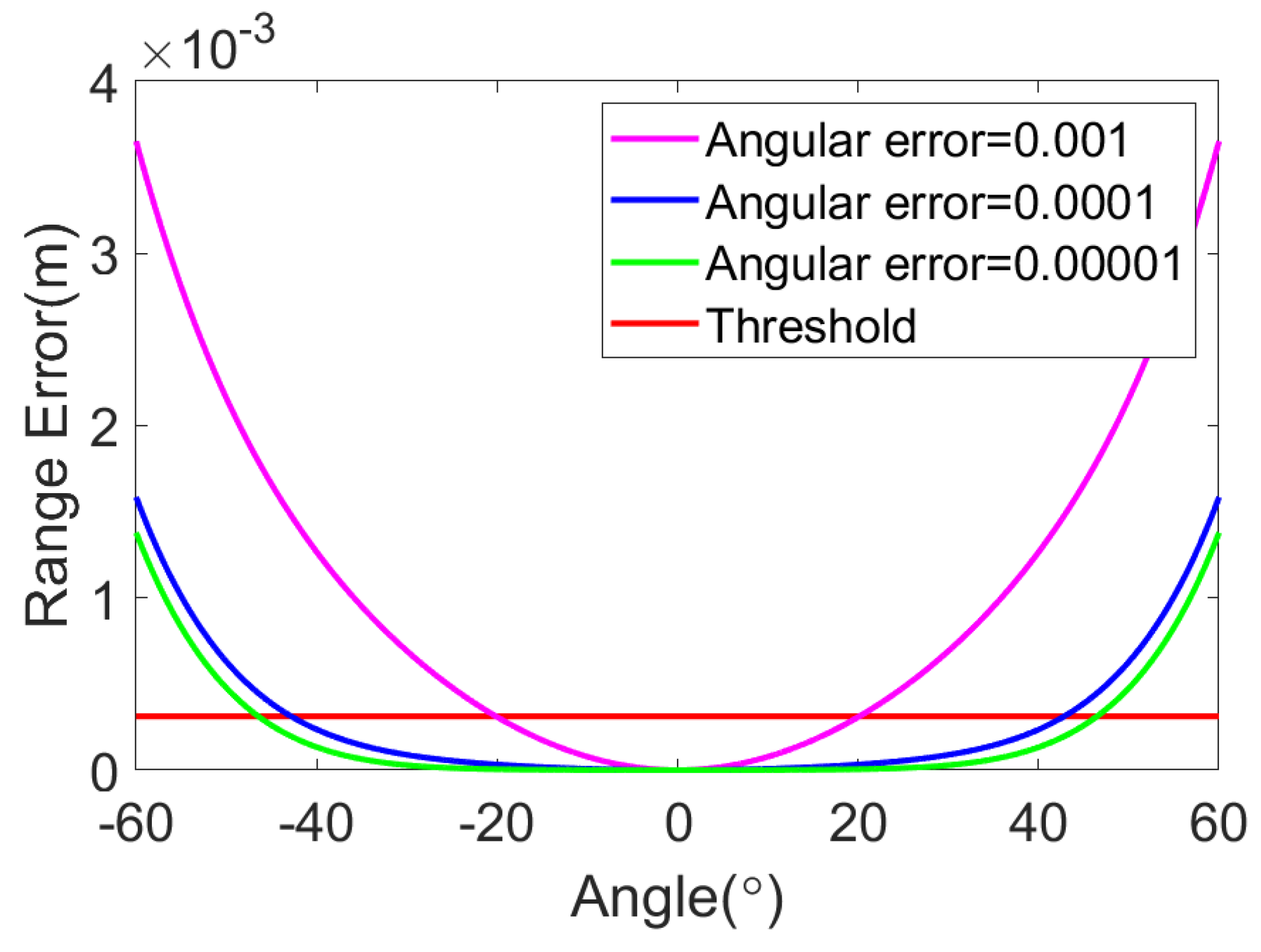
2.4.3. Imaging Error Analysis Based on Angular Sampling Error
2.4.4. Angular Sampling Error Analysis of Proposed System
3. Data and Experimental Results
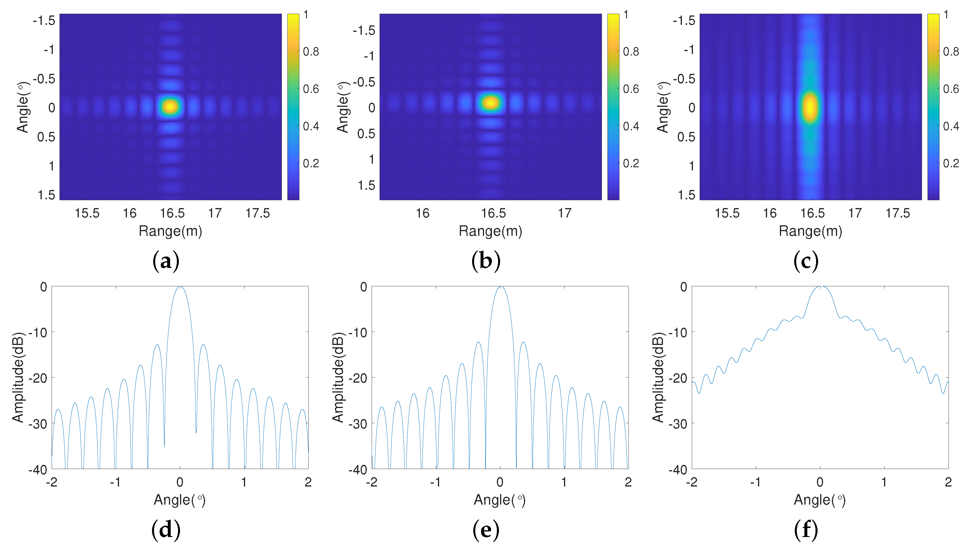
3.1. Simulation Experiment
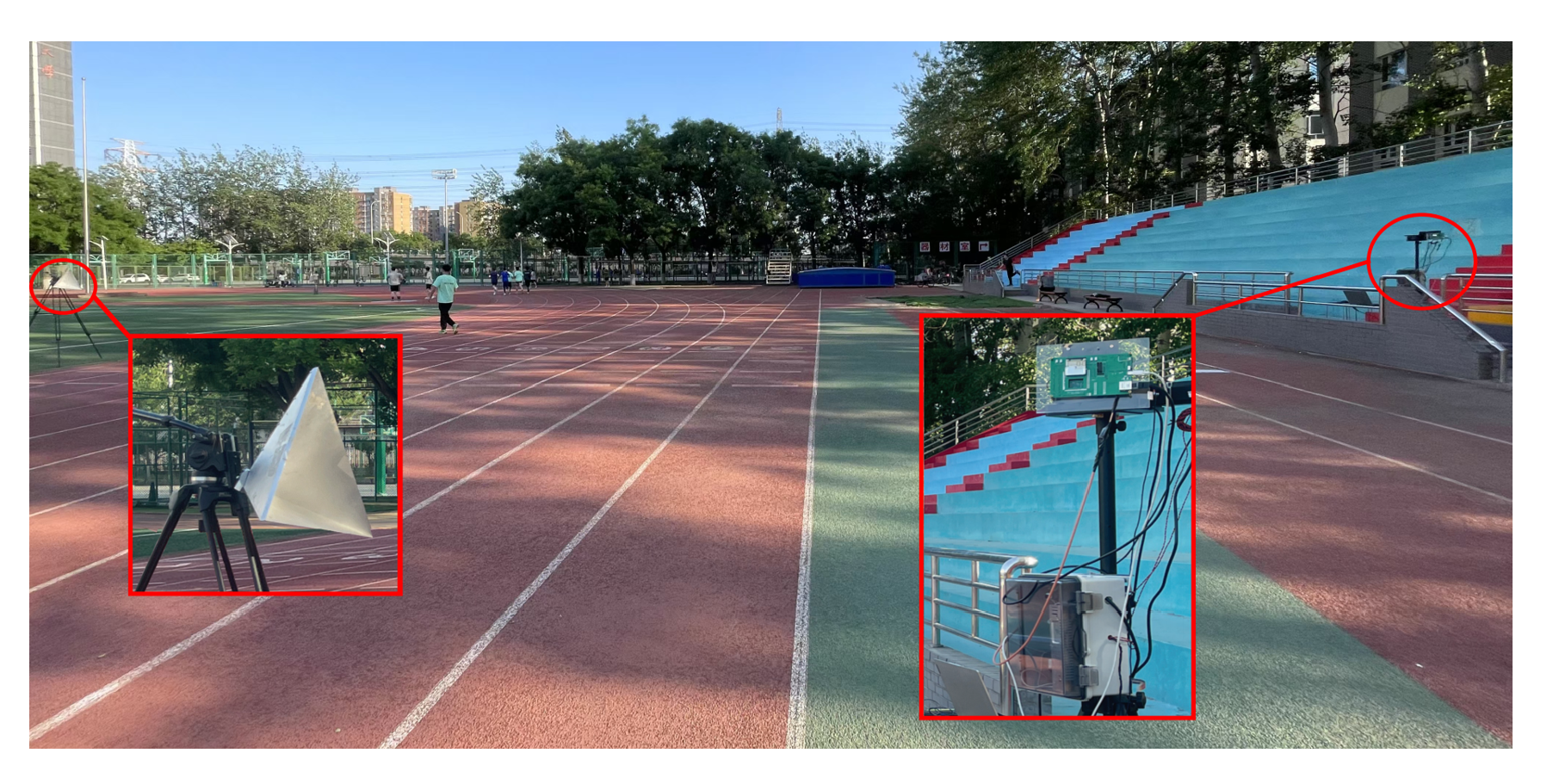
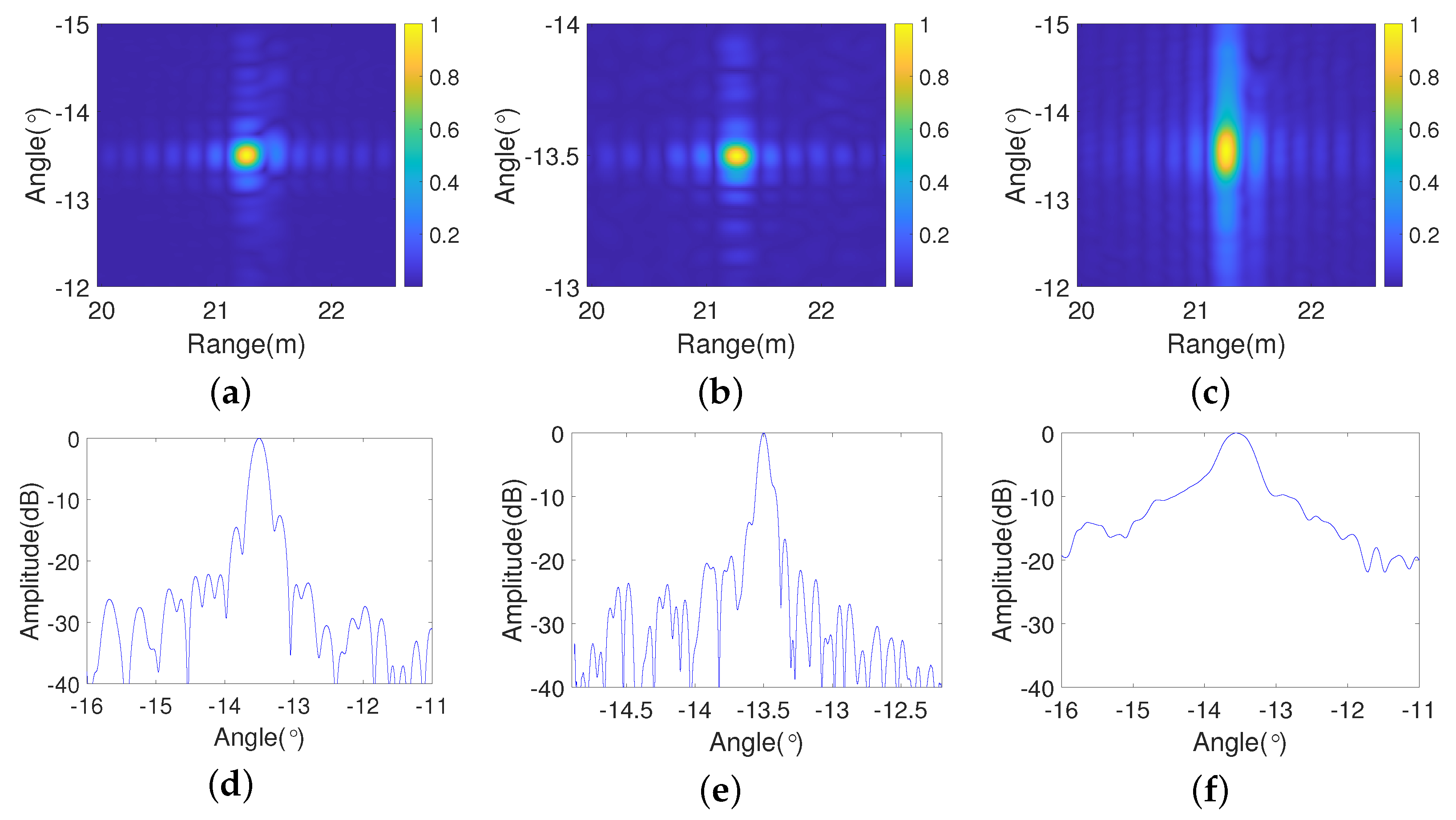
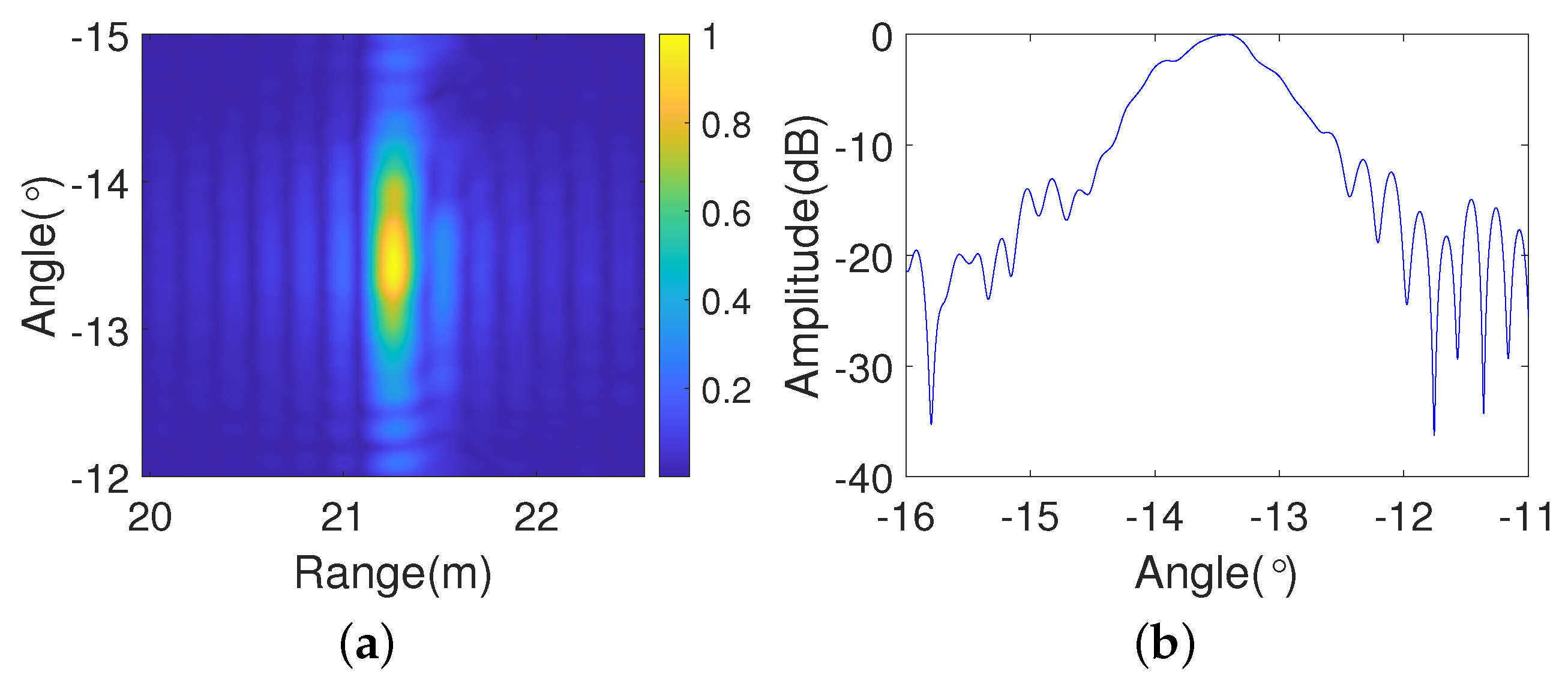
3.2. Real Experiment 1: Corner Reflector
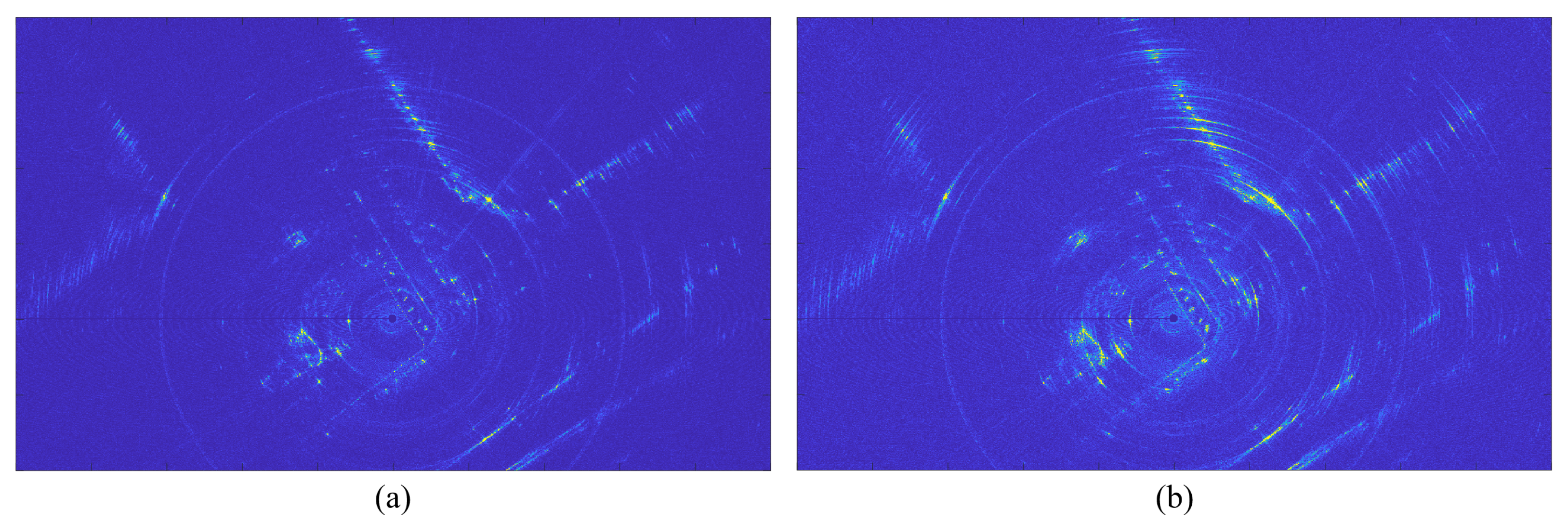
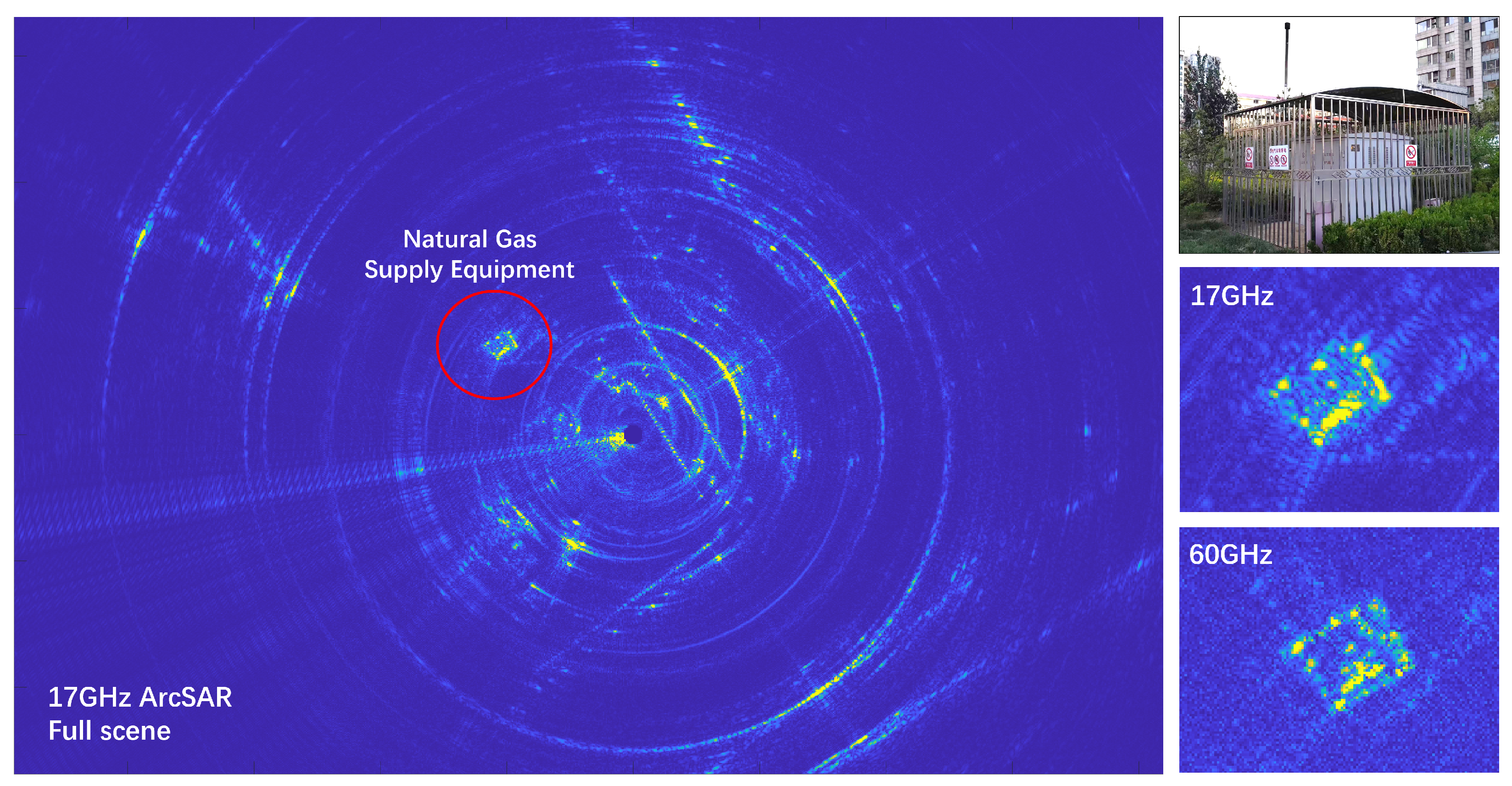
3.3. Real Experiment 2: Full-Aspect Imaging
4. Discussion
5. Conclusions
Author Contributions
Funding
Data Availability Statement
Acknowledgments
Conflicts of Interest
References
- Liang, D.; Zhang, H.; Fang, T.; Deng, Y.; Yu, W.; Zhang, L.; Fan, H. Processing of Very High Resolution GF-3 SAR Spotlight Data with Non-Start-Stop Model and Correction of Curved Orbit. IEEE J. Sel. Top. Appl. Earth Obs. Remote Sens. 2020, 13, 2112–2122. [Google Scholar] [CrossRef]
- Werninghaus, R.; Buckreuss, S. The TerraSAR-X Mission and System Design. IEEE Trans. Geosci. Remote Sens. 2010, 48, 606–614. [Google Scholar] [CrossRef]
- Martorella, M.; Pastina, D.; Berizzi, F.; Lombardo, P. Spaceborne Radar Imaging of Maritime Moving Targets With the Cosmo-SkyMed SAR System. IEEE J. Sel. Top. Appl. Earth Obs. Remote Sens. 2014, 7, 2797–2810. [Google Scholar] [CrossRef]
- Shen, W.; Lin, Y.; Li, Y.; Hong, W.; Wang, Y. Moving Targets Artifacts Removal in Multiaspect SAR Imagery Based on Logarithm Background Subtraction. IEEE J. Miniatur. Air Space Syst. 2023, 4, 62–69. [Google Scholar] [CrossRef]
- Hao, J.; Li, J.; Pi, Y.; Fang, X. A Drone Fleet-Borne SAR Model and Three-Dimensional Imaging Algorithm. IEEE Sens. J. 2019, 19, 9178–9186. [Google Scholar] [CrossRef]
- Appleby, R.; Anderton, R.N. Millimeter-Wave and Submillimeter-Wave Imaging for Security and Surveillance. Proc. IEEE 2007, 95, 1683–1690. [Google Scholar] [CrossRef]
- Wang, Y.; Hong, W.; Zhang, Y.; Lin, Y.; Li, Y.; Bai, Z.; Zhang, Q.; Lv, S.; Liu, H.; Song, Y. Ground-Based Differential Interferometry SAR: A Review. IEEE Geosci. Remote Sens. Mag. 2020, 8, 43–70. [Google Scholar] [CrossRef]
- Vu, V.T.; Sjogren, T.K.; Pettersson, M.I.; Gustavsson, A.; Ulander, L.M. Detection of moving targets by focusing in UWB SAR-Theory and experimental results. IEEE Trans. Geosci. Remote Sens. 2010, 48, 3799–3815. [Google Scholar] [CrossRef]
- Pieraccini, M.; Miccinesi, L. ArcSAR: Theory, Simulations, and Experimental Verification. IEEE Trans. Microw. Theory Tech. 2017, 65, 293–301. [Google Scholar] [CrossRef]
- Lin, Y.; Liu, Y.T.; Wang, Y.P.; Ye, S.B.; Zhang, Y.; Li, Y.; Li, W.; Qu, H.Q.; Hong, W. Frequency Domain Panoramic Imaging Algorithm for Ground-Based ArcSAR. Sensors 2020, 20, 7027. [Google Scholar] [CrossRef]
- Hua, Y.; Yang, Y.; Lu, B.; Cui, S.; Jiang, Z. Quantitative Analysis of Motion Effects on ArcSAR Panoramic Imaging Quality. In Proceedings of the 2024 9th International Conference on Signal and Image Processing (ICSIP), Nanjing, China, 12–14 July 2024; pp. 644–648. [Google Scholar] [CrossRef]
- Gao, Z.Y.; Jia, Y.; Liu, S.Y.; Zhang, X.K. Development of Ground-Based SFCW-ArcSAR System and Investigation on Point Target Response. Prog. Electromagn. Res. 2022, 109, 137–148. [Google Scholar] [CrossRef]
- Gao, Z.Y.; Jia, Y.; Liu, S.Y.; Zhang, X.K. A 2-D Frequency-Domain Imaging Algorithm for Ground-Based SFCW-ArcSAR. IEEE Trans. Geosci. Remote Sens. 2022, 60, 61660. [Google Scholar] [CrossRef]
- Fuentes, S.; Tongson, E.; Gonzalez Viejo, C. Urban Green Infrastructure Monitoring Using Remote Sensing from Integrated Visible and Thermal Infrared Cameras Mounted on a Moving Vehicle. Sensors 2021, 21, 295. [Google Scholar] [CrossRef] [PubMed]
- Ibrahim, M.R.; Lyons, T. Transforming CCTV cameras into NO2 sensors at city scale for adaptive policymaking. Sci. Rep. 2025, 15, 86532. [Google Scholar] [CrossRef]
- Schuetze, C.; Sauer, U. Challenges associated with the atmospheric monitoring of areal emission sources and the need for optical remote sensing techniques-an open-path Fourier transform infrared (OP-FTIR) spectroscopy experience report. Environ. Earth Sci. 2016, 75, 5482. [Google Scholar] [CrossRef]
- Tsuno, K.; Akahori, Y.; Yui, T.; Furukawa, H.; Watanabe, A.; Fujimaki, M.; Oto, M.; Katsuyama, T.; Iguchi, Y.; Inada, H.; et al. Highly-Sensitive Near-Infrared Spectroscopy System for Remote Monitoring of Concrete Structures. J. Disaster Res. 2017, 12, 536–545. [Google Scholar] [CrossRef]
- Wu, Y.C.; Noh, S.J.; Ham, S. Identification of Inundation Using Low-Resolution Images from Traffic-Monitoring Cameras: Bayes Shrink and Bayesian Segmentation. Water 2020, 12, 1725. [Google Scholar] [CrossRef]
- Xu, J.; Yu, X. The Immune Depth Presentation Convolutional Neural Network Used for Oil and Gas Pipeline Fault Diagnosis. IEEE Access 2024, 12, 163739–163751. [Google Scholar] [CrossRef]
- Yu, X.; Liang, X.; Zhou, Z.; Zhang, B.; Xue, H. Deep soft threshold feature separation network for infrared handprint identity recognition and time estimation. Infrared Phys. Technol. 2024, 138, 105223. [Google Scholar] [CrossRef]
- Yu, X.; Liang, X.J.; Zhou, Z.J.; Zhang, B.F. Multi-task learning for hand heat trace time estimation and identity recognition. Expert Syst. Appl. 2024, 255, 124551. [Google Scholar] [CrossRef]
- Wang, Y.; Sasamura, T.; Mustafa, A.; Morita, T. Real-time torque prediction for ultrasonic motors using an attention-based BiLSTM model and improved differential evolution algorithm. Measurement 2025, 251, 117266. [Google Scholar] [CrossRef]
- Broquetas, A.; De Porrata, R. Circular synthetic aperture radar (C-SAR) system for ground-based applications. Electron. Lett. 2002, 33, 988–989. [Google Scholar] [CrossRef]
- Yu, L.; Lin, Y.; Li, Y.; Wang, J.; Hong, W. Height Profile Estimation of Power Lines Based on Two-Dimensional CSAR Imagery. IEEE Geosci. Remote Sens. Lett. 2016, 13, 339–343. [Google Scholar] [CrossRef]
- Lee, H.; Lee, J.H.; Kim, K.E.; Sung, N.H.; Cho, S.J. Development of a Truck-Mounted Arc-Scanning Synthetic Aperture Radar. IEEE Trans. Geosci. Remote Sens. 2014, 52, 2773–2779. [Google Scholar] [CrossRef]
- Viviani, F.; Michelini, A.; Mayer, L.; Conni, F. IBIS-ArcSAR: An Innovative Ground-Based SAR System for Slope Monitoring. In Proceedings of the IGARSS 2018—2018 IEEE International Geoscience and Remote Sensing Symposium, Valencia, Spain, 22–27 July 2018; pp. 1348–1351. [Google Scholar] [CrossRef]
- Luo, Y.; Song, H.; Wang, R.; Deng, Y.; Zhao, F.; Xu, Z. Arc FMCW SAR and Applications in Ground Monitoring. IEEE Trans. Geosci. Remote Sens. 2014, 52, 5989–5998. [Google Scholar] [CrossRef]
- Ponce, O.; Prats, P.; Scheiber, R.; Reigber, A.; Moreira, A. Study of the 3-D Impulse Response Function of Holographic SAR Tomography with Multicircular Acquisitions. In Proceedings of the EUSAR 2014—0th European Conference on Synthetic Aperture Radar, Berlin, Germany, 3–5 June 2014; pp. 1–4. [Google Scholar]
- Cao, N.; Lee, H.; Zaugg, E.; Shrestha, R.; Carter, W.; Glennie, C.; Wang, G.; Lu, Z.; Fernandez-Diaz, J.C. Airborne DInSAR Results Using Time-Domain Backprojection Algorithm: A Case Study Over the Slumgullion Landslide in Colorado With Validation Using Spaceborne SAR, Airborne LiDAR, and Ground-Based Observations. IEEE J. Sel. Top. Appl. Earth Obs. Remote Sens. 2017, 10, 4987–5000. [Google Scholar] [CrossRef]
- Li, Z.; Wang, J.; Liu, Q.H. Frequency-Domain Backprojection Algorithm for Synthetic Aperture Radar Imaging. IEEE Geosci. Remote Sens. Lett. 2015, 12, 905–909. [Google Scholar] [CrossRef]
- Ash, J.N. An Autofocus Method for Backprojection Imagery in Synthetic Aperture Radar. IEEE Geosci. Remote Sens. Lett. 2012, 9, 104–108. [Google Scholar] [CrossRef]
- Gui, S.; Li, J.; Hao, J.; Zuo, F.; Pi, Y. Extension of Polar Format Algorithm to CSAR Imaging for Arbitrary Region of Interest. In Proceedings of the IGARSS 2019—2019 IEEE International Geoscience and Remote Sensing Symposium, Yokohama, Japan, 28 July–2 August 2019; pp. 2579–2582. [Google Scholar] [CrossRef]
- Wang, H.; Sun, B.; Li, C.; Jiang, Y.; Yang, W. An Improved Range-Doppler Imaging Algorithm Based on High-Order Range Model for Near-Field Panoramic Millimeter-Wave ArcSAR. IEEE Trans. Geosci. Remote Sens. 2023, 61, 5211016. [Google Scholar] [CrossRef]
- Ding, M.; Wang, X.; Wang, Y.; Dong, Q.; Tang, L.; Qu, J.; Liu, L.; Song, C.; Wang, B. First Demonstration of Metamaterial-Modulated Tag Localization and Imaging Based on K-Band FMCW Mini-SAR System. IEEE Trans. Microw. Theory Tech. 2024, 72, 6072–6082. [Google Scholar] [CrossRef]
- Jia, G.; Buchroithner, M.; Chang, W.; Li, X. Simplified Real-Time Imaging Flow for High-Resolution FMCW SAR. IEEE Geosci. Remote Sens. Lett. 2015, 12, 973–977. [Google Scholar] [CrossRef]
- Xu, L.; Lien, J.; Li, J. Doppler–Range Processing for Enhanced High-Speed Moving Target Detection Using LFMCW Automotive Radar. IEEE Trans. Aerosp. Electron. Syst. 2022, 58, 568–580. [Google Scholar] [CrossRef]
- Wang, S.; Guo, L.X.; Yu, Z.F.; Wang, J.; Chen, J. Method of 2-D Range-Doppler Imaging for Plasma Wake Based on Range Walk Correction. IEEE Trans. Plasma Sci. 2023, 51, 1076–1084. [Google Scholar] [CrossRef]
- Meta, A.; Hoogeboom, P.; Ligthart, L.P. Signal Processing for FMCW SAR. IEEE Trans. Geosci. Remote Sens. 2007, 45, 3519–3532. [Google Scholar] [CrossRef]
- Mittermayer, J.; Moreira, A.; Loffeld, O. Spotlight SAR data processing using the frequency scaling algorithm. IEEE Trans. Geosci. Remote Sens. 1999, 37, 2198–2214. [Google Scholar] [CrossRef]
- Neo, Y.L.; Wong, F.; Cumming, I.G. A Two-Dimensional Spectrum for Bistatic SAR Processing Using Series Reversion. IEEE Geosci. Remote Sens. Lett. 2007, 4, 93–96. [Google Scholar] [CrossRef]
- Neo, Y.L.; Wong, F.H.; Cumming, I.G. A Comparison of Point Target Spectra Derived for Bistatic SAR Processing. IEEE Trans. Geosci. Remote Sens. 2008, 46, 2481–2492. [Google Scholar] [CrossRef]
- de Wit, J.; Meta, A.; Hoogeboom, P. Modified range-Doppler processing for FM-CW synthetic aperture radar. IEEE Geosci. Remote Sens. Lett. 2006, 3, 83–87. [Google Scholar] [CrossRef]
- Huang, L.; Qiu, X.; Hu, D.; Han, B.; Ding, C. Medium-Earth-Orbit SAR Focusing Using Range Doppler Algorithm With Integrated Two-Step Azimuth Perturbation. IEEE Geosci. Remote Sens. Lett. 2015, 12, 626–630. [Google Scholar] [CrossRef]
- Berizzi, F.; Corsini, G. Autofocusing of inverse synthetic aperture radar images using contrast optimization. IEEE Trans. Aerosp. Electron. Syst. 1996, 32, 1185–1191. [Google Scholar] [CrossRef]
- Wang, J.; Liu, X. SAR Minimum-Entropy Autofocus Using an Adaptive-Order Polynomial Model. IEEE Geosci. Remote Sens. Lett. 2006, 3, 512–516. [Google Scholar] [CrossRef]


| Parameters | Symbol | Value |
|---|---|---|
| Carrier frequency | 60 GHz | |
| Bandwidth | 800 MHz | |
| Sampling rate | 12,500 Kps | |
| Number of range samples | 1024 | |
| Angular sampling interval | 0.0578° | |
| Linear frequency modulation | 10 MHz/μs | |
| Pulse duration | 30 μs | |
| Azimuth beamwidth | 64° | |
| Rotating radius | r | 0.52 m |
| Method | Point Target | Azimuth IRW (°) | Azimuth PLSR (dB) | Azimuth ISLR (dB) |
|---|---|---|---|---|
| Improved RD algorithm | (17 m, 0°) | 0.226 | −12.812 | −9.611 |
| BP Algorithm | (17 m, 0°) | 0.214 | −12.254 | −8.824 |
| Tradition RD algorithm | (17 m, 0°) | 0.218 | −7.160 | −1.934 |
| Method | Corner Reflector | Azimuth IRW (°) | Azimuth PLSR (dB) | Azimuth ISLR (dB) |
|---|---|---|---|---|
| Improved RD algorithm | 21.85 m | 0.201 | −12.563 | −10.681 |
| BP Algorithm | 21.85 m | 0.185 | −13.254 | −10.824 |
| Tradition RD algorithm | 21.85 m | 0.481 | −9.731 | −6.196 |
| Method | Scene 1 | Scene 2 | Scene 3 |
|---|---|---|---|
| Tradition RD algorithm | 2.73 s | 3.27 s | 2.69 s |
| Improved RD algorithm | 2.55 s | 3.62 s | 2.82 s |
| BP algorithm | 362.94 s | 362.81 s | 362.92 s |
| IC | IE | |||||
|---|---|---|---|---|---|---|
| Method | Scene 1 | Scene 2 | Scene 3 | Scene 1 | Scene 2 | Scene 3 |
| Tradition RD algorithm | 10.7481 | 8.2787 | 7.4753 | 8.9261 | 11.3765 | 8.3489 |
| Improved RD algorithm | 13.3066 | 15.059 | 8.9674 | 8.6094 | 10.9695 | 8.3378 |
| BP algorithm | 14.0141 | 17.7937 | 10.0552 | 8.5395 | 10.946 | 7.7565 |
Disclaimer/Publisher’s Note: The statements, opinions and data contained in all publications are solely those of the individual author(s) and contributor(s) and not of MDPI and/or the editor(s). MDPI and/or the editor(s) disclaim responsibility for any injury to people or property resulting from any ideas, methods, instructions or products referred to in the content. |
© 2025 by the authors. Licensee MDPI, Basel, Switzerland. This article is an open access article distributed under the terms and conditions of the Creative Commons Attribution (CC BY) license (https://creativecommons.org/licenses/by/4.0/).
Share and Cite
Shen, W.; Lv, W.; Wang, Y.; Lin, Y.; Li, Y.; Bai, Z.; Yu, K. High-Resolution Wide-Beam Millimeter-Wave ArcSAR System for Urban Infrastructure Monitoring. Remote Sens. 2025, 17, 2043. https://doi.org/10.3390/rs17122043
Shen W, Lv W, Wang Y, Lin Y, Li Y, Bai Z, Yu K. High-Resolution Wide-Beam Millimeter-Wave ArcSAR System for Urban Infrastructure Monitoring. Remote Sensing. 2025; 17(12):2043. https://doi.org/10.3390/rs17122043
Chicago/Turabian StyleShen, Wenjie, Wenxing Lv, Yanping Wang, Yun Lin, Yang Li, Zechao Bai, and Kuai Yu. 2025. "High-Resolution Wide-Beam Millimeter-Wave ArcSAR System for Urban Infrastructure Monitoring" Remote Sensing 17, no. 12: 2043. https://doi.org/10.3390/rs17122043
APA StyleShen, W., Lv, W., Wang, Y., Lin, Y., Li, Y., Bai, Z., & Yu, K. (2025). High-Resolution Wide-Beam Millimeter-Wave ArcSAR System for Urban Infrastructure Monitoring. Remote Sensing, 17(12), 2043. https://doi.org/10.3390/rs17122043