
Automated Local Climate Zone Mapping via Multi-Parameter Synergistic Optimization and High-Resolution GIS-RS Fusion


Abstract
1. Introduction
- Inadequate adaptation to spatial heterogeneity: The block-based method proposed in [29] for Xi’an struggles to capture intra-block heterogeneity; AutoLCZ employs uniform grids, which are not adaptive to morphological gradients; and although the Berlin method attempts to identify transition zones using k-means, it fails to address the issue of spatial autocorrelation.
- Lack of multi-parameter synergistic constraints: LCZ classification requires satisfying multiple threshold conditions simultaneously. AutoLCZ extracts only a limited set of parameters from LiDAR data; the method applied in Xi’an relies heavily on manual judgment; and the Berlin GIS-LCZ approach considers seven parameters, but lacks a mechanism for considering synergistic constraints among them.
- Trade-off between computational efficiency and classification accuracy: The Xi’an method involves significant manual intervention; AutoLCZ depends on high-quality LiDAR data; and the fuzzy logic algorithm in the Berlin GIS-LCZ approach has high computational complexity and strong data dependency. None of the three methods effectively balances efficiency and accuracy. In addition, the Istanbul study emphasizes that both remote sensing image quality and annotation accuracy have a significant impact on the model’s performance.
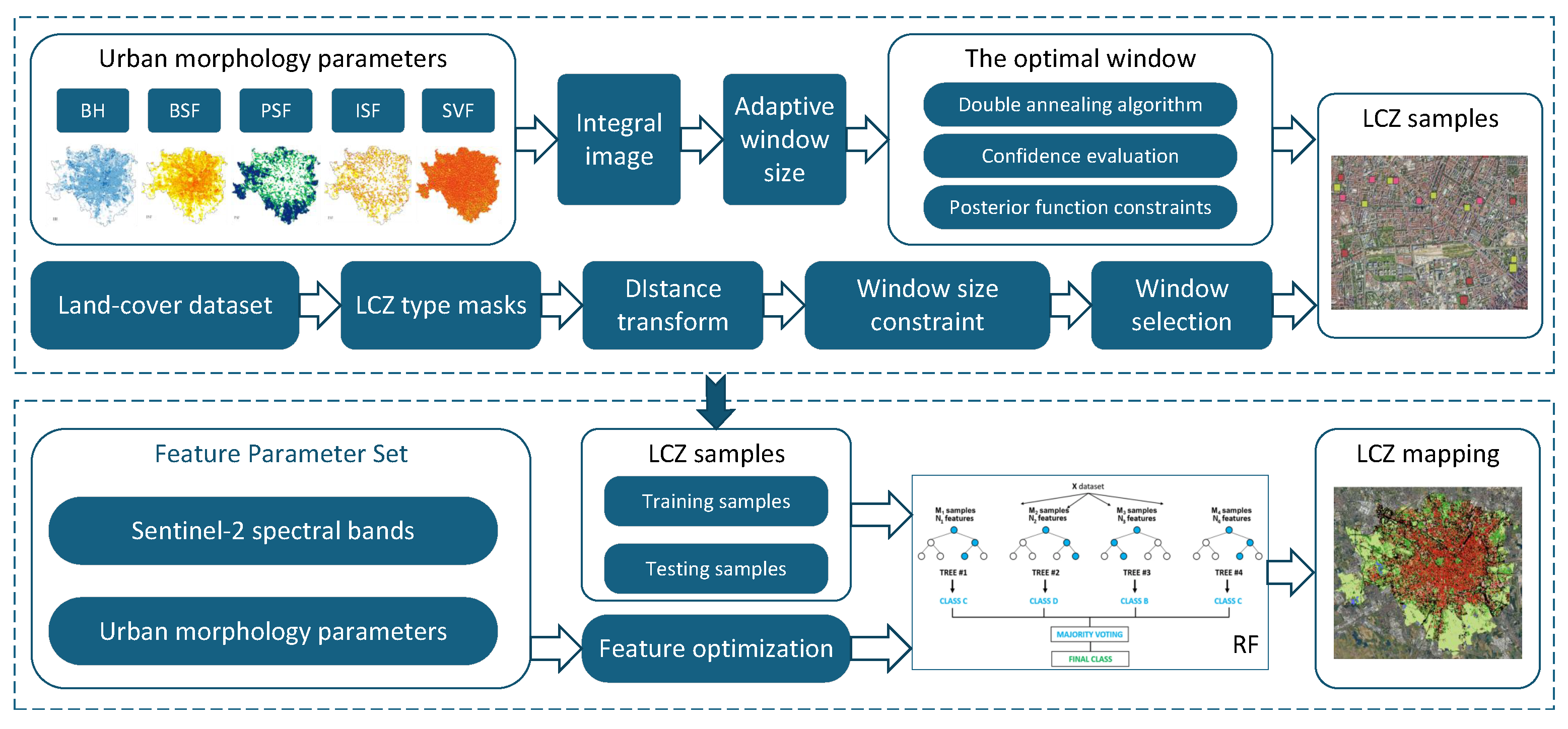
- First, a multi-parameter Synergistic Optimization-based window selection strategy is proposed for built LCZ types. By employing multi-objective function evaluation and Pareto front screening, the method achieves optimal sample selection under the coordinated constraints of multiple urban morphological parameters. Furthermore, a dynamic threshold adjustment mechanism and a three-stage global-to-local fine-tuning strategy are introduced to effectively address the parameter conflicts and spatial heterogeneity inherent in traditional methods.
- Second, a Distance-driven Maximum Coverage method is developed for land-cover LCZ types. Based on land-use classification data, this method utilizes chessboard distance transformation and boundary constraints to generate candidate sampling windows. It prioritizes the selection of large, non-overlapping areas, significantly enhancing spatial coverage diversity and computational efficiency.
- Third, this study is the first to integrate Pareto front screening with a dynamic tolerance mechanism to mitigate premature convergence in multi-objective optimization. This innovation ensures robust and adaptive parameter optimization for built-up LCZ sample generation. The proposed dual-path framework balances strict morphological constraints with optimized spatial coverage, contributing to scalable, automated, and high-quality LCZ sample production at a global scale.
2. Materials and Methods
2.1. Materials
2.1.1. Study Area
2.1.2. Data
2.2. Urban Morphological Parameters (UMPs)
- (1)
- Building Height (BH)The mean building height refers to the geometric mean height of buildings within an analysis unit. It is a key parameter used to identify high-rise areas (BH > 25 m), mid-rise areas (BH = 15–25 m), or low-rise areas (BH < 15 m).where represents the building height, and n is the count of buildings within the unit.
- (2)
- Building Surface Fraction (BSF)The building surface fraction is the ratio of the total building area within a unit to the total unit area. BSF is a critical parameter for distinguishing compact urban areas (BSF > 0.4) from open urban areas (BSF < 0.4).where represents the area of buildings, and is the area of the unit.
- (3)
- Pervious Surface Fraction (PSF)The pervious surface fraction is the ratio of the total pervious area within a unit to the total unit area. Pervious surfaces include land-use types such as vegetation, bare soil, and water. In this study, PSF was calculated based on the sum of water and vegetation areas from land-use data provided by the ESA.where represents the area of pervious surface, and is the area of the unit.
- (4)
- Impervious Surface Fraction (ISF)The impervious surface fraction refers to the ratio of the total impervious area within a unit to the total unit area. Here, impervious surfaces exclude building areas. ISF in this study was calculated using impervious surface area data provided by Wuhan University.where represents the area of the impervious surface, and is the area of the unit.
- (5)
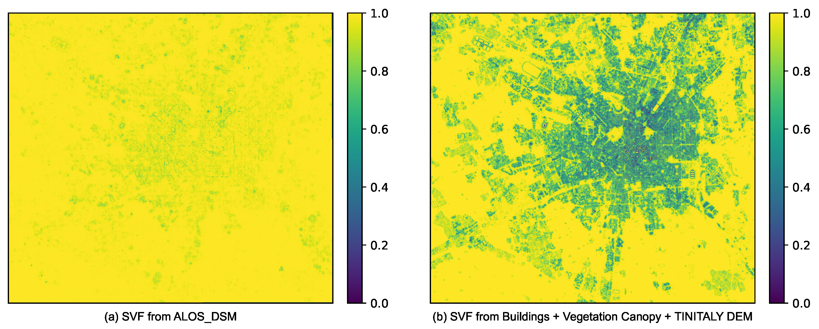
- Sky View Factor (SVF)The sky view factor is the average ratio of the visible sky hemisphere from the ground, with values ranging from 0 to 1. In this study, SVF was calculated using DSM data for terrain, the global canopy height data, and building data, input into the System for Automated Geoscientific Analyses (SAGA) software [41]. The input parameters were set to their default values: a maximum search radius of 100 units and 16 directional sectors.
2.3. Methods
- (1)
- Design of the Optimization Objective Function
- Threshold adherence ensures that the mean values within each window align with the predefined LCZ class ranges, with a dynamic tolerance ($T_tol$) enhancing adaptability;
- Spatial uniformity constrains the local feature space by minimizing the variance within the window to ensure internal consistency;
- Window shape regularity restricts the window aspect ratio () and enforces a minimum area () to avoid irregular geometries;
- The overlap constraint prohibits overlap between windows of different LCZ classes, while allowing only minimal overlap among windows of the same class.
- (2)
- Composite Scoring Function for Candidate Solutions
- The optimization confidence reflects the performance of the candidate in the objective function optimization process, defined as the inverse of the loss value;
- The threshold coverage represents the proportion of spectral bands within the window that meet the predefined LCZ threshold conditions;
- The shape score penalizes deviations from an ideal rectangular form based on the aspect ratio;
- The threshold adherence calculates the weighted distance between band means and the center of threshold ranges to assess sample representativeness.
- Dynamic variance constraint: To enhance local refinement, a dynamic threshold is applied to the standard deviation of each spectral band. The 85th percentile of global candidates’ variance distributions is used to define the maximum allowable standard deviation (max_std), effectively filtering out noisy candidates while maintaining sufficient sampling diversity. This approach strikes a balance between avoiding overly strict thresholds that may lead to sample scarcity, and avoiding overly lenient thresholds that may introduce noise.
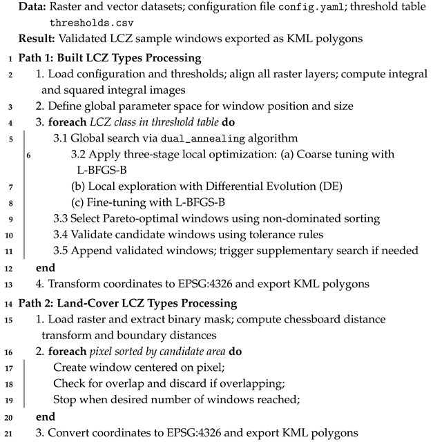
- Hybrid Optimization Strategy: To further enhance the precision of candidate window refinement, this study introduces a three-stage local optimization mechanism. First, the L-BFGS-B algorithm is employed to perform rapid bounded optimization on initial candidate windows, ensuring spatial validity through explicit constraints [47]. If the resulting confidence is insufficient, a Differential Evolution (DE) algorithm is introduced to perform a global search and escape from local optima. Finally, L-BFGS-B is applied again to finely adjust the DE results with high precision, ensuring strict compliance with LCZ-specific prior constraints such as parameter consistency and geometric regularity.
- Pareto-based candidate selection: To simultaneously satisfy multiple objectives—statistical, geometric, and spatial—this study adopts a Pareto-optimal selection strategy [48]. By using non-dominated sorting and Pareto front extraction, candidate windows are evaluated based on the mean error, variance, coverage rate, and aspect ratio. This avoids subjective weighting and preserves optimal candidates that balance feature representation and geometric regularity. The parameter settings are listed in Appendix A, Table A1.
| Algorithm 1: Dual-path Framework for Automated LCZ Sample Generation |
 |
3. Results
3.1. LCZ Map Validation
3.2. LCZ Mapping Results
4. Discussion
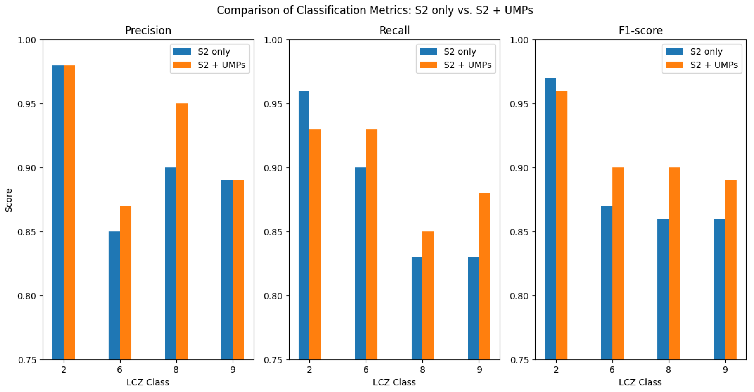
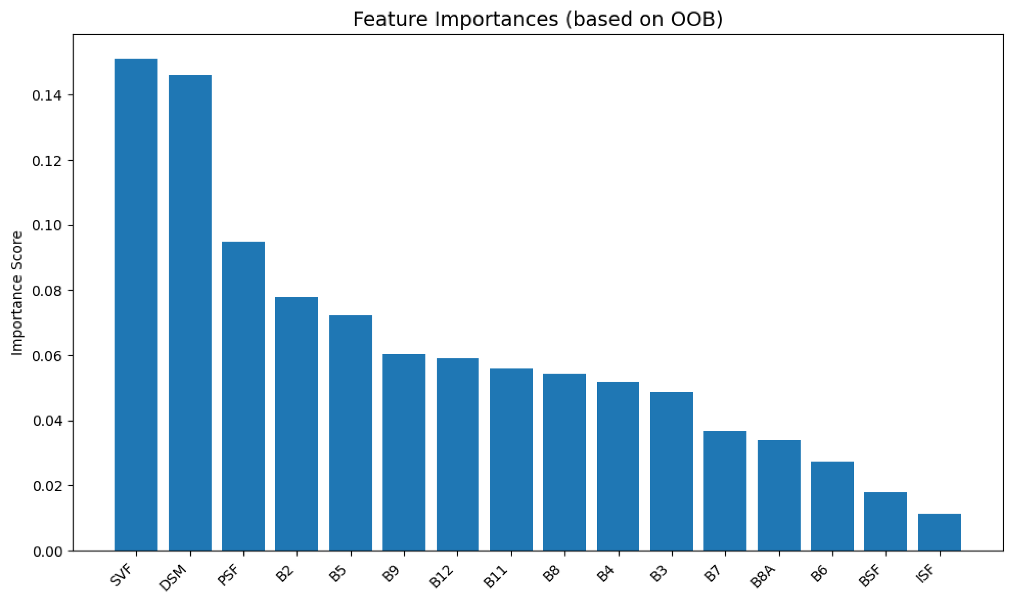
4.1. The Influence of High-Resolution UMPs on the Construction of LCZ Samples
4.2. Interpretation of the LCZ Mapping Results
4.3. Scalability and Generalizability to Diverse Urban Forms
4.4. Challenges and Prospects of Automated LCZ Sample Generation
5. Conclusions
- Methodological innovation: This study is the first to combine Pareto front screening with a dynamic tolerance mechanism, effectively addressing the problem of premature convergence in multi-objective optimization. The proposed dual-pathway framework demonstrates strong adaptability and high accuracy in generating samples for both urban and land-cover LCZ types.
- Advantages of data fusion: By integrating high-resolution GIS data (specifically, urban morphological parameters) with RS imagery, the framework significantly enhances sample representativeness. This confirms the core value of high-resolution datasets in supporting automated LCZ construction.
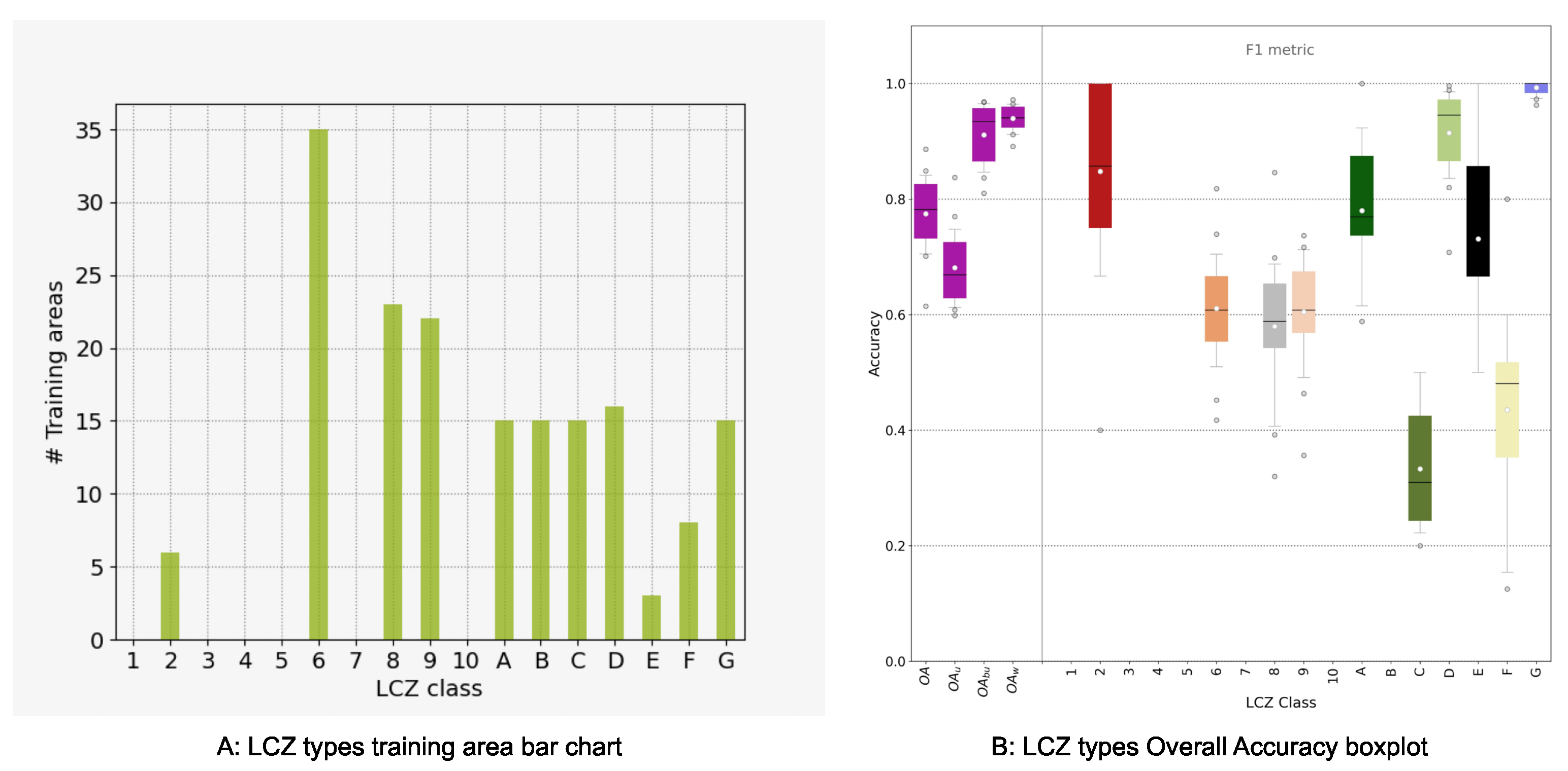
- Outstanding classification performance: In the case study of Milan, the overall classification accuracy reached 95.3%, with stable performance in typical urban types such as LCZ 2, 6, 8, and 9, indicating strong discriminatory power across different urban functional zones.
Author Contributions
Funding
Data Availability Statement
Acknowledgments
Conflicts of Interest
Appendix A

| Parameter Type | Parameter Name | Value | Usage |
|---|---|---|---|
| Global Parameters | HUGE_PENALTY | A penalty value is applied to invalid solutions (e.g., constraint violations) to force the optimizer away from infeasible regions | |
| LOCAL_REFINE_THRESHOLD | 0.5 | The confidence threshold for triggering local refinement; activates the three-stage local optimization if the confidence is below this value | |
| MAX_WINDOW_RATIO | 2.0 | The maximum allowed aspect ratio of a sampling window to avoid overly elongated shapes (e.g., ratio > 2:1) | |
| MIN_WINDOW_AREA | 100 | The minimum window area (in pixels); filters out excessively small candidate windows | |
| SHAPE_WEIGHT | 50.0 | The shape penalty weight; applies a linear penalty to windows exceeding the aspect ratio limit | |
| UNIFORMITY_REWARD_WEIGHT | 0.05 | The reward weight for spatial uniformity; encourages low-variance windows | |
| COVERAGE_THRESHOLD | 1 | The posterior validation threshold: requires 100% of bands to meet their respective mean constraints | |
| ALLOWED_OVERLAP_RATIO | 0 | The maximum allowed overlap ratio for same-class windows (0 indicates strict non-overlapping) | |
| LAMBDA_ADHERENCE | 1.0 | The weight for threshold adherence; emphasizes the closeness between band means and the threshold center in the composite score | |
| Custom Parameters | MAX_ITERATIONS | 500 | The maximum number of iterations for the dual annealing algorithm during the global search phase |
| CANDIDATE_CONFIDENCE | 0.9 | The minimum confidence threshold for candidate solutions; candidates below this value are discarded | |
| MIN_CONFIDENCE | 0.05 | The lower confidence bound for retaining candidate solutions to avoid over-filtering | |
| VAR_WEIGHT | 0.05 | The weight assigned to variance error in the objective function (balanced with the weight for mean error) | |
| MEAN_PENALTY_WEIGHT | 8.0 | The penalty weight for mean deviation; controls the sensitivity of the objective function to deviations from threshold means | |
| MAX_STD | – | The initial maximum allowed standard deviation for each band (prior to dynamic adjustment), corresponding to SVF:0.5, BSF:0.5, ISF:0.55, PSF:0.6, and BH:15.0 respectively. | |
| Adaptive parameters | EFFECTIVE_MAX_STD | 85th | Dynamically constrains within-window uniformity by excluding the top 15% of high-variance outliers |
| TOL_FACTOR | 0.15 | The dynamic tolerance range for posterior mean validation, allowing slight deviation from the threshold (e.g., ±15%) |
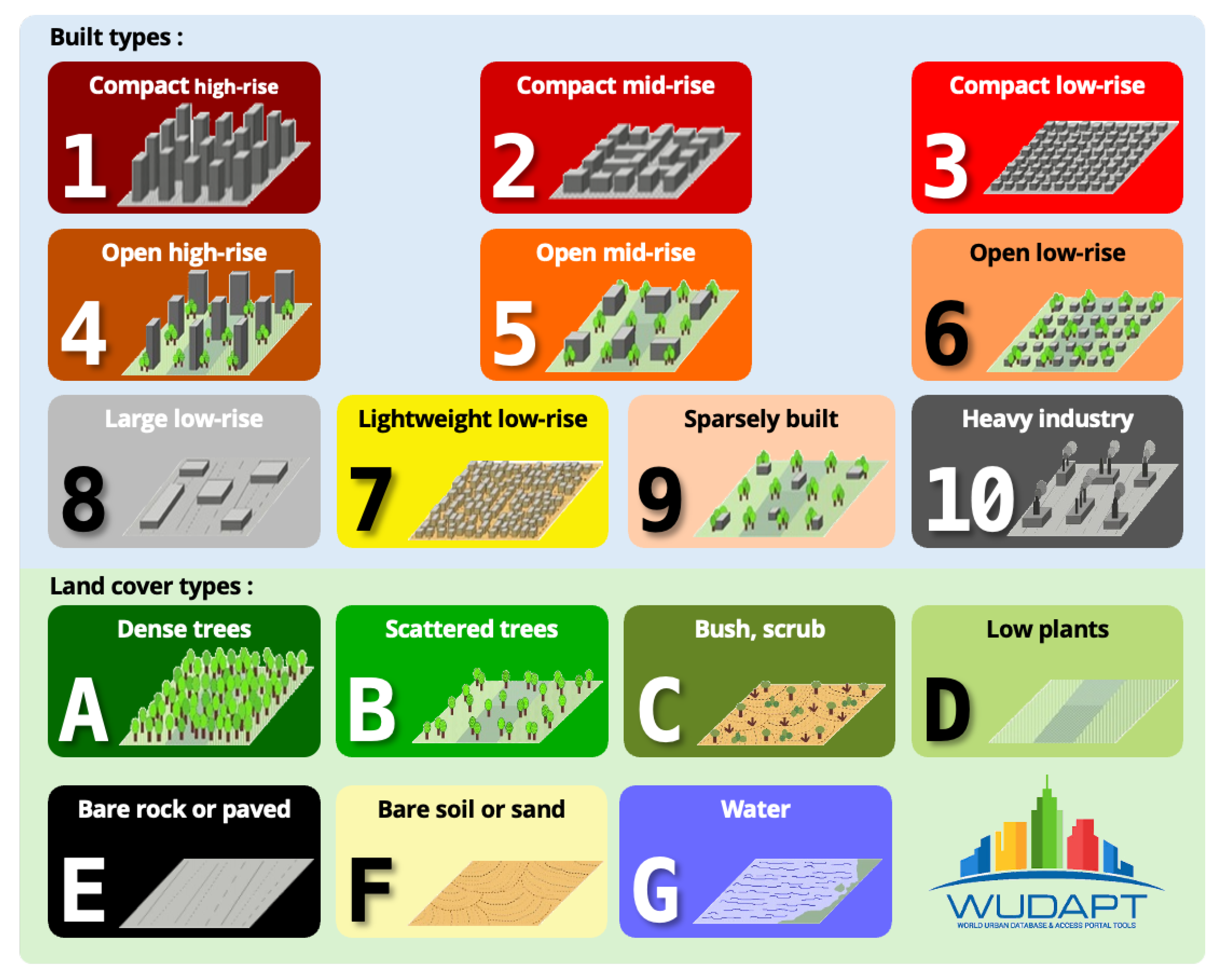
| LCZ Code | Name | Description |
|---|---|---|
| 1 | Compact high-rise | Dense, tall buildings with little vegetation |
| 2 | Compact mid-rise | Dense, mid-height buildings with limited vegetation |
| 3 | Compact low-rise | Dense, low buildings with paved surfaces |
| 4 | Open high-rise | Tall buildings with open spacing and vegetation |
| 5 | Open mid-rise | Mid-height buildings with moderate open space |
| 6 | Open low-rise | Detached low buildings with vegetation |
| 7 | Lightweight low-rise | Informal or temporary low buildings |
| 8 | Large low-rise | Industrial or commercial buildings with large footprints |
| 9 | Sparsely built | Scattered buildings with substantial open land |
| 10 | Heavy industry | Large-scale industrial complexes |
| A | Dense trees | Forests or wooded areas with closed canopy |
| B | Scattered trees | Open tree cover with grass or bare soil |
| C | Bush, scrub | Shrubs, low woody plants, sparse trees |
| D | Low plants | Grasslands, herbaceous vegetation |
| E | Bare rock or paved | Hard, non-vegetated surfaces |
| F | Bare soil or sand | Loose soil, sand, or dry ground |
| G | Water | Rivers, lakes, reservoirs, and other water bodies |
References
- United Nations. World Urbanization Prospects: The 2014 Revision, Highlights; Department of Economic and Social Affairs, Population Division, United Nations: New York, NY, USA, 2014; Volume 32. [Google Scholar]
- Acuto, M.; Parnell, S.; Seto, K.C. Building a Global Urban Science. Nat. Sustain. 2018, 1, 2–4. [Google Scholar] [CrossRef]
- Collier, C.G. The Impact of Urban Areas on Weather. Q. J. R. Meteorol. Soc. 2006, 132, 1–25. [Google Scholar] [CrossRef]
- Miao, S.; Chen, F.; Li, Q.; Fan, S. Impacts of Urban Processes and Urbanization on Summer Precipitation: A Case Study of Heavy Rainfall in Beijing on 1 August 2006. J. Appl. Meteorol. Climatol. 2011, 50, 806–825. [Google Scholar] [CrossRef]
- Oke, T.R.; Mills, G.; Christen, A.; Voogt, J.A. Urban Climates; Cambridge University Press: Cambridge, UK, 2017. [Google Scholar]
- Sun, Y.; Zhang, X.; Ren, G.; Zwiers, F.W.; Hu, T. Contribution of Urbanization to Warming in China. Nat. Clim. Chang. 2016, 6, 706–709. [Google Scholar] [CrossRef]
- Yan, Z.W.; Wang, J.; Xia, J.J.; Feng, J.M. Review of Recent Studies of the Climatic Effects of Urbanization in China. Adv. Clim. Chang. Res. 2016, 7, 154–168. [Google Scholar] [CrossRef]
- Manoli, G.; Fatichi, S.; Schläpfer, M.; Yu, K.; Crowther, T.W.; Meili, N.; Burlando, P.; Katul, G.G.; Bou-Zeid, E. Magnitude of Urban Heat Islands Largely Explained by Climate and Population. Nature 2019, 573, 55–60. [Google Scholar] [CrossRef]
- Oke, T.R. Initial Guidance to Obtain Representative Meteorological Observations at Urban Sites; World Meteorological Organization: Geneva, Switzerland, 2004; Volume 81. [Google Scholar]
- Ellefsen, R. Mapping and Measuring Buildings in the Canopy Boundary Layer in Ten U.S. Cities. Energy Build. 1991, 16, 1025–1049. [Google Scholar] [CrossRef]
- Davenport, A.G.; Grimmond, C.S.B.; Oke, T.R.; Wieringa, J. Estimating the Roughness of Cities and Sheltered Country. In Proceedings of the 12th Conference on Applied Climatology, Ashville, NC, USA, 8–11 May 2000; Volume 96, p. 99. [Google Scholar]
- Stewart, I.D.; Oke, T.R. Local Climate Zones for Urban Temperature Studies. Bull. Am. Meteorol. Soc. 2012, 93, 1879–1900. [Google Scholar] [CrossRef]
- Demuzere, M.; Hankey, S.; Mills, G.; Zhang, W.; Lu, T.; Bechtel, B. Combining Expert and Crowd-Sourced Training Data to Map Urban Form and Functions for the Continental US. Sci. Data 2020, 7, 264. [Google Scholar] [CrossRef]
- Bechtel, B.; Demuzere, M.; Mills, G.; Zhan, W.; Sismanidis, P.; Small, C.; Voogt, J. SUHI Analysis Using Local Climate Zones—A Comparison of 50 Cities. Urban Clim. 2019, 28, 100451. [Google Scholar] [CrossRef]
- Liu, Y.; Li, Q.; Yang, L.; Mu, K.; Zhang, M.; Liu, J. Urban Heat Island Effects of Various Urban Morphologies under Regional Climate Conditions. Sci. Total Environ. 2020, 743, 140589. [Google Scholar] [CrossRef]
- Das, M.; Das, A. Exploring the Pattern of Outdoor Thermal Comfort (OTC) in a Tropical Planning Region of Eastern India during Summer. Urban Clim. 2020, 34, 100708. [Google Scholar] [CrossRef]
- Patel, P.; Jamshidi, S.; Nadimpalli, R.; Aliaga, D.G.; Mills, G.; Chen, F.; Demuzere, M.; Niyogi, D. Modeling Large-Scale Heatwave by Incorporating Enhanced Urban Representation. J. Geophys. Res. Atmos. 2022, 127, e2021JD035316. [Google Scholar] [CrossRef]
- Liu, L.; Liu, J.; Jin, L.; Liu, L.; Gao, Y.; Pan, X. Climate-Conscious Spatial Morphology Optimization Strategy Using a Method Combining Local Climate Zone Parameterization Concept and Urban Canopy Layer Model. Build. Environ. 2020, 185, 107301. [Google Scholar] [CrossRef]
- Vandamme, S.; Demuzere, M.; Verdonck, M.L.; Zhang, Z.; Van Coillie, F. Revealing Kunming’s (China) Historical Urban Planning Policies through Local Climate Zones. Remote Sens. 2019, 11, 1731. [Google Scholar] [CrossRef]
- Shi, Y.; Ren, C.; Lau, K.K.L.; Ng, E. Investigating the Influence of Urban Land Use and Landscape Pattern on PM2.5 Spatial Variation Using Mobile Monitoring and WUDAPT. Landsc. Urban Plan. 2019, 189, 15–26. [Google Scholar] [CrossRef]
- Brousse, O.; Georganos, S.; Demuzere, M.; Vanhuysse, S.; Wouters, H.; Wolff, E.; Linard, C.; van Lipzig, N.P.M.; Dujardin, S. Using Local Climate Zones in Sub-Saharan Africa to Tackle Urban Health Issues. Urban Clim. 2019, 27, 227–242. [Google Scholar] [CrossRef]
- Yang, X.; Peng, L.L.H.; Chen, Y.; Yao, L.; Wang, Q. Air Humidity Characteristics of Local Climate Zones: A Three-Year Observational Study in Nanjing. Build. Environ. 2020, 171, 106661. [Google Scholar] [CrossRef]
- Mills, G.; Ching, J.; See, L.; Bechtel, B.; Foley, M. An Introduction to the WUDAPT Project. In Proceedings of the 9th International Conference on Urban Climate, Toulouse, France, 20–24 July 2015; pp. 20–24. [Google Scholar]
- Kim, M.; Jeong, D.; Kim, Y. Local Climate Zone Classification Using a Multi-Scale, Multi-Level Attention Network. ISPRS J. Photogramm. Remote Sens. 2021, 181, 345–366. [Google Scholar] [CrossRef]
- Wu, Q.; Ma, X.; Sui, J.; Pun, M.O. DF4LCZ: A SAM-Empowered Data Fusion Framework for Scene-Level Local Climate Zone Classification. IEEE Trans. Geosci. Remote Sens. 2024, 62, 5406216. [Google Scholar] [CrossRef]
- Zheng, Y.; Ren, C.; Xu, Y.; Wang, R.; Ho, J.; Lau, K.; Ng, E. GIS-based Mapping of Local Climate Zone in the High-Density City of Hong Kong. Urban Clim. 2018, 24, 419–448. [Google Scholar] [CrossRef]
- Hidalgo, J.; Dumas, G.; Masson, V.; Petit, G.; Bechtel, B.; Bocher, E.; Foley, M.; Schoetter, R.; Mills, G. Comparison between Local Climate Zones Maps Derived from Administrative Datasets and Satellite Observations. Urban Clim. 2019, 27, 64–89. [Google Scholar] [CrossRef]
- Muhammad, F.; Xie, C.; Vogel, J.; Afshari, A. Inference of Local Climate Zones from GIS Data, and Comparison to WUDAPT Classification and Custom-Fit Clusters. Land 2022, 11, 747. [Google Scholar] [CrossRef]
- Xu, D.; Zhang, Q.; Zhou, D.; Yang, Y.; Wang, Y.; Rogora, A. Local Climate Zone in Xi’an City: A Novel Classification Approach Employing Spatial Indicators and Supervised Classification. Buildings 2023, 13, 2806. [Google Scholar] [CrossRef]
- Liu, C.; Song, H.; Shreevastava, A.; Albrecht, C.M. AutoLCZ: Towards Automatized Local Climate Zone Mapping from Rule-Based Remote Sensing. In Proceedings of the IGARSS 2024—2024 IEEE International Geoscience and Remote Sensing Symposium, Athens, Greece, 7–12 July 2024; pp. 2023–2027. [Google Scholar] [CrossRef]
- Nicancı Sinanoğlu, M.; Kaya, Ş. Local Climate Zone Classification Using YOLOV8 Modeling in Instance Segmentation Method. Int. J. Environ. Geoinform. 2024, 11, 1–9. [Google Scholar] [CrossRef]
- Islam, M.D.; Di, L.; Zhang, C.; Yang, R.; Qu, J.J.; Tong, D.; Guo, L.; Lin, L.; Pandey, A. A Decision Rule and Machine Learning-Based Hybrid Approach for Automated Land-Cover Type Local Climate Zones (LCZs) Mapping Using Multi-Source Remote Sensing Data. IEEE J. Sel. Top. Appl. Earth Obs. Remote Sens. 2024, 17, 8271–8290. [Google Scholar] [CrossRef]
- Milojevic-Dupont, N.; Wagner, F.; Nachtigall, F.; Hu, J.; Brüser, G.B.; Zumwald, M.; Biljecki, F.; Heeren, N.; Kaack, L.H.; Pichler, P.P.; et al. EUBUCCO v0.1: European Building Stock Characteristics in a Common and Open Database for 200+ Million Individual Buildings. Sci. Data 2023, 10, 147. [Google Scholar] [CrossRef]
- Copernicus Land Monitoring Service. CLCplus Backbone 2021 (Raster 10 m), Europe, 3-Yearly, Jun. 2024; European Environment Agency: Copenhagen, Denmark, 2024. [Google Scholar] [CrossRef]
- Tolan, J.; Yang, H.I.; Nosarzewski, B.; Couairon, G.; Vo, H.V.; Brandt, J.; Spore, J.; Majumdar, S.; Haziza, D.; Vamaraju, J.; et al. Very High Resolution Canopy Height Maps from RGB Imagery Using Self-Supervised Vision Transformer and Convolutional Decoder Trained on Aerial Lidar. Remote Sens. Environ. 2024, 300, 113888. [Google Scholar] [CrossRef]
- Tarquini, S.; Isola, I.; Favalli, M.; Battistini, A.; Dotta, G. TINITALY, a Digital Elevation Model of Italy with a 10 Meters Cell Size (Version 1.1); Istituto Nazionale di Geofisica e Vulcanologia (INGV): Roma, Italy, 2023. [Google Scholar]
- European Space Agency. Sentinel-2 MSI: MultiSpectral Instrument, Level-2A. Available online: https://developers.google.com/earth-engine/datasets/catalog/COPERNICUS_S2_SR_HARMONIZED (accessed on 14 April 2025).
- Copernicus Land Monitoring Service. Impervious Built-up 2018 (Raster 10 m), Europe, 3-Yearly, Aug. 2020; European Environment Agency: Copenhagen, Denmark, 2020. [Google Scholar] [CrossRef]
- Quan, J. Enhanced Geographic Information System-Based Mapping of Local Climate Zones in Beijing, China. Sci. China Technol. Sci. 2019, 62, 2243–2260. [Google Scholar] [CrossRef]
- Yonghuan, M.A.; Linlin, L.U.; Da, X.; Meng, C.A.I.; Chao, R.E.N.; Meiling, Z.; Wenhua, H.U.I.; Qingting, L.I. Urban Thermal Environment Analysis by Local Climate Zone in Beijing. J. Beijing Norm. Univ. (Nat. Sci.) 2022, 58, 901–909. [Google Scholar]
- Conrad, O.; Bechtel, B.; Bock, M.; Dietrich, H.; Fischer, E.; Gerlitz, L.; Wehberg, J.; Wichmann, V.; Böhner, J. System for Automated Geoscientific Analyses (SAGA) v. 2.1.4. Geosci. Model Dev. 2015, 8, 1991–2007. [Google Scholar] [CrossRef]
- Viola, P.; Jones, M. Rapid Object Detection Using a Boosted Cascade of Simple Features. In Proceedings of the 2001 IEEE Computer Society Conference on Computer Vision and Pattern Recognition, CVPR 2001, Kauai, HI, USA, 8–14 December 2001; Volume 1, pp. I-511–I-518. [Google Scholar] [CrossRef]
- Demuzere, M.; Bechtel, B.; Middel, A.; Mills, G. Mapping Europe into Local Climate Zones. PLoS ONE 2019, 14, e0214474. [Google Scholar] [CrossRef]
- Xiang, Y.; Sun, D.Y.; Fan, W.; Gong, X.G. Generalized Simulated Annealing Algorithm and Its Application to the Thomson Model. Phys. Lett. A 1997, 233, 216–220. [Google Scholar] [CrossRef]
- Abouelsaad, O.; Hassan, A.; Omar, M.; Hinkelmann, R. Identifying Manning Roughness Coefficient Using Automatic Calibration Method and Simulation of Pollution Incidents in the Nile River, Egypt. J. Hydrol. Reg. Stud. 2024, 55, 101908. [Google Scholar] [CrossRef]
- Soonjun, B.; Krityakierne, T. GDESA: Gradient Differential Evolution-Simulated Annealing Hybrid. IEEE Access 2024, 12, 165555–165581. [Google Scholar] [CrossRef]
- Kästner, J.; Sherwood, P. Superlinearly Converging Dimer Method for Transition State Search. J. Chem. Phys. 2008, 128, 014106. [Google Scholar] [CrossRef] [PubMed]
- Li, X.; Gao, B.; Pan, Y.; Bai, Z.; Gao, Y.; Dong, S.; Li, S. Multi-Objective Optimization Sampling Based on Pareto Optimality for Soil Mapping. Geoderma 2022, 425, 116069. [Google Scholar] [CrossRef]
- Belgiu, M.; Drăguţ, L. Random Forest in Remote Sensing: A Review of Applications and Future Directions. ISPRS J. Photogramm. Remote Sens. 2016, 114, 24–31. [Google Scholar] [CrossRef]
- Mushore, T.D.; Dube, T.; Manjowe, M.; Gumindoga, W.; Chemura, A.; Rousta, I.; Odindi, J.; Mutanga, O. Remotely Sensed Retrieval of Local Climate Zones and Their Linkages to Land Surface Temperature in Harare Metropolitan City, Zimbabwe. Urban Clim. 2019, 27, 259–271. [Google Scholar] [CrossRef]
- Chung, L.C.H.; Xie, J.; Ren, C. Improved Machine-Learning Mapping of Local Climate Zones in Metropolitan Areas Using Composite Earth Observation Data in Google Earth Engine. Build. Environ. 2021, 199, 107879. [Google Scholar] [CrossRef]
- Huang, F.; Jiang, S.; Zhan, W.; Bechtel, B.; Liu, Z.; Demuzere, M.; Huang, Y.; Xu, Y.; Ma, L.; Xia, W.; et al. Mapping Local Climate Zones for Cities: A Large Review. Remote Sens. Environ. 2023, 292, 113573. [Google Scholar] [CrossRef]
- Breiman, L. Bagging Predictors. Mach. Learn. 1996, 24, 123–140. [Google Scholar] [CrossRef]
- Demuzere, M.; Kittner, J.; Bechtel, B. LCZ Generator: A Web Application to Create Local Climate Zone Maps. Front. Environ. Sci. 2021, 9, 637455. [Google Scholar] [CrossRef]
- Bechtel, B.; Alexander, P.J.; Beck, C.; Böhner, J.; Brousse, O.; Ching, J.; Demuzere, M.; Fonte, C.; Gál, T.; Hidalgo, J.; et al. Generating WUDAPT Level 0 Data–Current Status of Production and Evaluation. Urban Clim. 2019, 27, 24–45. [Google Scholar] [CrossRef]
- Vavassori, A.; Oxoli, D.; Venuti, G.; Brovelli, M.A.; Siciliani de Cumis, M.; Sacco, P.; Tapete, D. A Combined Remote Sensing and GIS-based Method for Local Climate Zone Mapping Using PRISMA and Sentinel-2 Imagery. Int. J. Appl. Earth Obs. Geoinf. 2024, 131, 103944. [Google Scholar] [CrossRef]
- Tadono, T.; Nagai, H.; Ishida, H.; Oda, F.; Naito, S.; Minakawa, K.; Iwamoto, H. Generation of the 30 M-Mesh Global Digital Surface Model by Alos Prism. Int. Arch. Photogramm. Remote Sens. Spat. Inf. Sci. 2016, XLI-B4, 157–162. [Google Scholar] [CrossRef]


| Data | Time | Data Type | Resolution | Source | Usage |
|---|---|---|---|---|---|
| Building Dataset | 2022 | Vector | – | EUBUCCO [33] | Building location, building area, calculation of BH and BSF |
| CLCplus Backbone | 2021 | Raster | 10 m | ESA [34] | Classification of land-cover LCZ types, calculation of PSF |
| TINITALY DEM | 2023 | Raster | 10 m | INGV [36] | Calculation of SVF |
| Global Canopy Height Maps | 2009–2020 | Raster | 1 m | Meta and WRI [35] | Calculation of SVF |
| Sentinel 2 Image | 2020–2021 | Raster | 10 m | ESA [37] | Band features used for classification |
| Impervious Built-Up | 2018 | Raster | 10 m | ESA [38] | Calculation of ISF |
| LCZ | SVF | BSF (%) | ISF (%) | PSF (%) | MBH (m) |
|---|---|---|---|---|---|
| LCZ 1 | 0.2–0.4 | 40–60 | 40–60 | <10 | ≥25 |
| LCZ 2 | 0.3–0.6 | 40–70 | 30–50 | <20 | 10–<25 |
| LCZ 3 | 0.2–0.6 | 40–70 | 20–50 | <30 | 3–<10 |
| LCZ 4 | 0.5–0.7 | 20–40 | 30–40 | 30–40 | ≥25 |
| LCZ 5 | 0.5–0.8 | 20–40 | 30–50 | 20–40 | 10–<25 |
| LCZ 6 | 0.6–0.9 | 20–40 | 20–50 | 30–60 | 3–<10 |
| LCZ 7 | 0.2–0.5 | 60–90 | <20 | <30 | 2–4 |
| LCZ 8 | >0.7 | 30–50 | 40–50 | <20 | 3–<10 |
| LCZ 9 | >0.8 | 10–20 | <20 | 60–80 | 3–<10 |
| LCZ 10 | 0.6–0.9 | 20–30 | 20–40 | 40–50 | 5–<15 |
| LCZ A–G | Defined by land-use classification | ||||
| Metric | 2 | 6 | 8 | 9 | A | B | C | D | E | F | G |
|---|---|---|---|---|---|---|---|---|---|---|---|
| Precision | 0.98 | 0.87 | 0.95 | 0.89 | 0.95 | 1.00 | 0.97 | 0.99 | 0.97 | 0.93 | 1.00 |
| Recall | 0.93 | 0.93 | 0.85 | 0.88 | 0.98 | 0.62 | 0.74 | 1.00 | 0.87 | 0.84 | 1.00 |
| F1-score | 0.96 | 0.90 | 0.90 | 0.89 | 0.97 | 0.76 | 0.84 | 0.99 | 0.92 | 0.89 | 1.00 |
| LCZ Types | Proposed | From [56] | ||||
|---|---|---|---|---|---|---|
| Precision | Recall | F1-Score | Precision | Recall | F1-Score | |
| 2 | 0.98 | 0.93 | 0.96 | 0.82 | 0.89 | 0.85 |
| 3 | – | – | – | 0.77 | 0.73 | 0.75 |
| 5 | – | – | – | 0.77 | 0.78 | 0.78 |
| 6 | 0.87 | 0.93 | 0.90 | 0.82 | 0.78 | 0.80 |
| 8 | 0.95 | 0.85 | 0.90 | 0.98 | 0.99 | 0.99 |
| 9 | 0.89 | 0.88 | 0.89 | – | – | – |
| A | 0.95 | 0.98 | 0.97 | 0.98 | 0.73 | 0.84 |
| B | 1.00 | 0.62 | 0.76 | 0.83 | 0.93 | 0.88 |
| C | 0.97 | 0.74 | 0.84 | – | – | – |
| D | 0.99 | 1.00 | 0.99 | 0.98 | 0.92 | 0.95 |
| E | 0.97 | 0.87 | 0.92 | 0.93 | 0.97 | 0.95 |
| F | 0.93 | 0.84 | 0.89 | 0.90 | 0.99 | 0.94 |
| G | 1.00 | 1.00 | 1.00 | 1.00 | 1.00 | 1.00 |
| Overall Accuracy | 0.95 | 0.88 | ||||
Disclaimer/Publisher’s Note: The statements, opinions and data contained in all publications are solely those of the individual author(s) and contributor(s) and not of MDPI and/or the editor(s). MDPI and/or the editor(s) disclaim responsibility for any injury to people or property resulting from any ideas, methods, instructions or products referred to in the content. |
© 2025 by the authors. Licensee MDPI, Basel, Switzerland. This article is an open access article distributed under the terms and conditions of the Creative Commons Attribution (CC BY) license (https://creativecommons.org/licenses/by/4.0/).
Share and Cite
Li, W.; Liu, X.; Samat, A.; Gamba, P. Automated Local Climate Zone Mapping via Multi-Parameter Synergistic Optimization and High-Resolution GIS-RS Fusion. Remote Sens. 2025, 17, 2038. https://doi.org/10.3390/rs17122038
Li W, Liu X, Samat A, Gamba P. Automated Local Climate Zone Mapping via Multi-Parameter Synergistic Optimization and High-Resolution GIS-RS Fusion. Remote Sensing. 2025; 17(12):2038. https://doi.org/10.3390/rs17122038
Chicago/Turabian StyleLi, Wenbo, Ximing Liu, Alim Samat, and Paolo Gamba. 2025. "Automated Local Climate Zone Mapping via Multi-Parameter Synergistic Optimization and High-Resolution GIS-RS Fusion" Remote Sensing 17, no. 12: 2038. https://doi.org/10.3390/rs17122038
APA StyleLi, W., Liu, X., Samat, A., & Gamba, P. (2025). Automated Local Climate Zone Mapping via Multi-Parameter Synergistic Optimization and High-Resolution GIS-RS Fusion. Remote Sensing, 17(12), 2038. https://doi.org/10.3390/rs17122038