Temporal and Spatial Analysis of the Impact of the 2015 St. Patrick’s Day Geomagnetic Storm on Ionospheric TEC Gradients and GNSS Positioning in China Using GIX and ROTI Indices

Abstract

Geomagnetic storms induce ionospheric disturbances, significantly affecting Global Navigation Satellite System (GNSS) positioning accuracy. This study investigates how geomagnetic storm-induced ionospheric irregularities influence GNSS Precise Point Positioning (PPP), using data from approximately 260 GNSS stations across China during 15 storm events between 1 January and 30 June 2015. We applied two indices—the Gradient Ionosphere Index (GIX), representing spatial gradients of vertical total electron content (VTEC), and the Rate of TEC Index (ROTI), describing temporal TEC variations. The analysis identified the St. Patrick’s Day geomagnetic storm (17 March 2015) as causing the most pronounced ionospheric disruptions, with significant east–west TEC gradients (|GIXx,P95| > 50 mTECU/km) consistently associated with substantial PPP errors (>0.5 m). Spatial analyses further indicated that significant 3D PPP errors (PPP, P₉₅ > 0.4 m) closely overlapped with regions experiencing intense east–west TEC gradients, predominantly in the 20–35°N latitude band. Further analysis indicated notable pre-storm ionospheric enhancements driven by zonal electric fields, distinct ionospheric suppression associated with westward disturbance dynamo electric fields (DDEFs) on 18 March, and re-intensification due to eastward penetration electric fields (PEFs) on 19 March.

1. Introduction

Geomagnetic storms are triggered by solar activities such as coronal mass ejections and solar flares. These storms can significantly perturb the Earth’s ionosphere, leading to irregular fluctuations in ionospheric electron density known as ionospheric scintillations [1,2]. These scintillations can cause sudden and rapid changes in the amplitude and phase of GNSS signals, resulting in cycle slips, loss of lock, and degradation of positioning and navigation accuracy [3,4].

One factor thought to be contributing to ionospheric scintillations is the inhomogeneity of ionospheric electron distribution, characterized by spatial plasma density or total electron content (TEC) gradients [5]. Numerous studies indicate that the strength of the spatial gradient of TEC has adverse effects on GNSS positioning, including Precise Point Positioning (PPP). For example, Jakowski [6] found that pronounced horizontal TEC gradients can significantly impede the resolution of phase ambiguities in precise geodetic and surveying networks. Nava [7] discussed the contribution of horizontal gradients of vertical TEC (VTEC) to positioning errors. In addition, considerable research has examined the potential risks posed by strong spatial TEC gradients in life-safety applications for air traffic management, as well as their influence on errors in both absolute and relative GNSS positioning [7,8,9]. To analyze ionospheric perturbations and assess their influence on GNSS positioning, various indices have been developed. The Rate of Total Electron Content Index (ROTI) and Gradient Ionospheric Index (GIX) have been used to identify signals severely affected by the ionospheric gradient [10,11]. ROTI, which incorporates both the spatial and temporal gradients of TEC variations as per its definition [5,12], has been widely employed as a reliable measure to evaluate the existence of ionospheric irregularities and assess the frequency of ionospheric scintillations [13,14]. However, because ROTI combines spatial and temporal variability, it can be challenging to distinguish between these effects without detailed TEC mapping [6]. To overcome this limitation, the GIX was proposed to rapidly obtain absolute changes in the horizontal TEC gradient [11].

Ionospheric irregularities—such as the Equatorial Ionization Anomaly (EIA), Tongue of Ionization (TOI), and storm-time features like Storm-Enhanced Density (SED)—are closely associated with such TEC gradients, as they are characterized by rapid spatial and temporal variations in electron density [5,15,16]. Numerous studies have explored the link between TEC gradients and ionospheric irregularities. For instance, Vo and Foster [17] conducted a quantitative analysis of ionospheric density gradients and found that the strongest gradients often occur at the boundaries of narrow structures such as the SED—especially between its polar edge and the equatorward edge of the Main Ionospheric Trough (MIT); Klimenko et al. [18] stated that the TOI creates sharp electron density gradients at its edges, which can significantly disrupt GNSS signal propagation and positioning accuracy; Dugassa et al. [5] found that spatial TEC gradients observed during the postsunset period in the equatorial region over Ethiopia are closely associated with the development of ionospheric irregularities, particularly equatorial plasma bubbles; and Zhang et al. [19] investigated spatial TEC gradients under geomagnetic perturbations and suggested that significant storm-time electron density redistribution leads to enhanced TEC gradients, which coincide with regions of increased ionospheric irregularities.

Moreover, during intense geomagnetic storms—such as the 17 March 2015 St. Patrick’s Day storm, the most severe of solar cycle 24—these irregularities become substantially amplified. This amplification results in steeper TEC gradients and can cause severe degradation in GNSS positioning accuracy [18,20]. Additionally, observations over Europe confirmed that the GIX effectively captured the rapidly evolving spatial gradients of VTEC [11,21]. While previous research has discussed the effects of ionospheric irregularities induced by geomagnetic storms on precise GNSS positioning during the 2015 St. Patrick’s Day magnetic storm [22,23,24], a gap still remains in understanding the temporal and spatial characteristics of ionospheric gradients, particularly for high-precision GNSS positioning in China. Furthermore, existing research has predominantly utilized indices like ROTI to monitor ionospheric irregularities. However, ROTI’s ability to distinguish between spatial and temporal TEC gradients is limited, making it difficult to accurately represent the precise physical characteristics of irregularities [25]. This limitation suggests the need for more precise tools, such as GIX, which can provide a clearer depiction of horizontal TEC gradient changes [11]. Therefore, there remains a need for studies that integrate both temporal and spatial analyses of ionospheric TEC gradients to enhance the understanding of their impact on high-precision GNSS positioning.

This study aims to address the existing gap by conducting a detailed temporal and spatial analysis of the impact of geomagnetic storms on ionospheric gradients and GNSS positioning in China, using both the GIX and ROTI indices. Based on observations from approximately 260 GNSS stations across China between 1 January and 30 June 2015, we first analyzed the temporal behavior of ionospheric TEC gradients. We then analyzed how the March 2015 St. Patrick’s Day storm altered horizontal TEC gradients and caused large kinematic PPP errors across China. This research provides a more comprehensive understanding of the spatial distribution and gradient variations in ionospheric disturbances during geomagnetic storms, supporting the development of strategies to mitigate their adverse effects on GNSS positioning accuracy.

2. Data and Methods

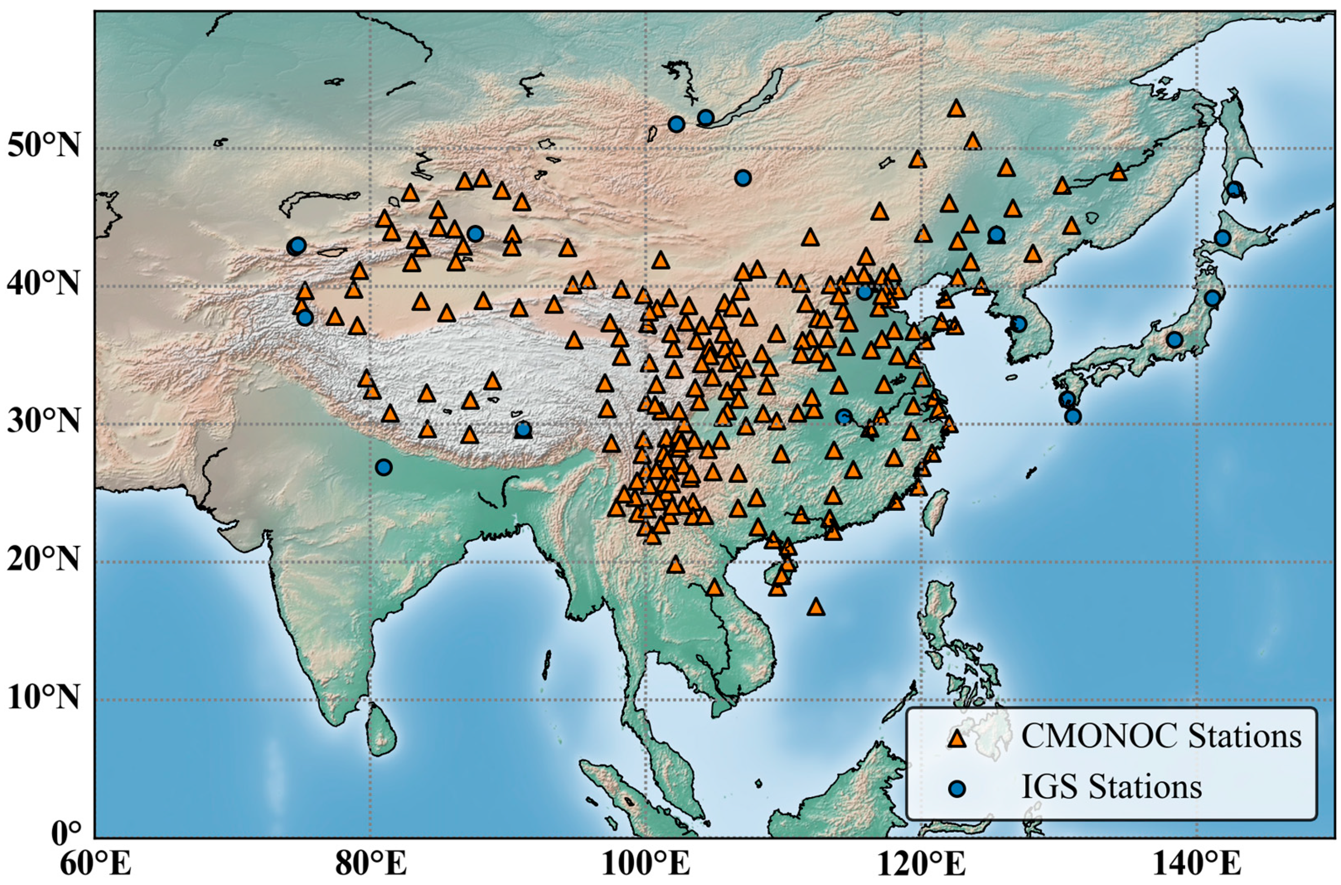
2.1. GNSS Data and Processing

GNSS observation data were obtained from 240 stations of the Crustal Movement Observation Network of China (CMONOC) and 19 stations from the International GNSS Service (IGS). The geographical distribution of these stations is illustrated in Figure 1. Due to an interruption in data reception from CMONOC stations after 1 July 2015, we only collected CMONOC and IGS data between 1 January and 30 June 2015. We analyzed 15 geomagnetic storm events, including 4 strong geomagnetic storms and 11 moderate geomagnetic storms. These events occurred between 1 January and 30 June 2015. The minimum Dst index values recorded during these geomagnetic events ranged from −52 nT to −234 nT (17 March 2015).

The GNSS data comprise pseudorange and phase observations sampled every 30 s, providing measurements of raw ionospheric Slant Total Electron Content (STEC) for characterizing ionospheric density along the line of sight. The $\mathrm{S}\mathrm{T}\mathrm{E}\mathrm{C}$ can be expressed as follows:

$$\left\{\begin{array}{l}\mathsf{S}\mathsf{T}\mathsf{E}{\mathrm{C}}_{\mathrm{r}\mathrm{e}\mathrm{l}}={\displaystyle \frac{1}{40.3}}\left({\displaystyle \frac{{\mathrm{f}}_1^2·{\mathrm{f}}_2^2}{{\mathrm{f}}_1^2-{\mathrm{f}}_2^2}}\right)\left({\mathrm{P}}_2-{\mathrm{P}}_1+{\mathrm{D}\mathrm{C}\mathrm{B}}^{\mathrm{s}}+{\mathrm{D}\mathrm{C}\mathrm{B}}_{\mathrm{r}}\right)\\ \mathsf{S}\mathsf{T}\mathsf{E}\mathsf{C}=\mathsf{S}\mathsf{T}\mathsf{E}{\mathrm{C}}_{\mathrm{r}\mathrm{e}\mathrm{l}}-\mathsf{D}\mathsf{C}{\mathrm{B}}_{\mathrm{r}}-\mathsf{D}\mathsf{C}{\mathrm{B}}^{\mathrm{s}}\end{array}\right.$$

(1)

where $\mathrm{S}\mathrm{T}\mathrm{E}{\mathrm{C}}_{\mathrm{r}\mathrm{e}\mathrm{l}}$ represents the relative line-of-sight total electron content (STEC, in TECU). $\mathrm{S}\mathrm{T}\mathrm{E}\mathrm{C}$ denotes the bias-free STEC, while ${\mathrm{f}}_1$ and ${\mathrm{f}}_2$ represent the frequencies (in MHz) associated with the phase observations. ${\mathrm{P}}_1$ and ${\mathrm{P}}_2$ are GNSS pseudoranges. ${\mathrm{D}\mathrm{C}\mathrm{B}}^{\mathrm{s}}$ and ${\mathrm{D}\mathrm{C}\mathrm{B}}_{\mathrm{r}}$ are the satellite Differential Code Bias (DCB) and receiver DCB, respectively.

A code-smoothing strategy was applied for each continuous observation arc to obtain high-precision ionospheric TEC measurements [26]. Absolute STEC values are obtained by routinely computing the DCBs for both satellite and receiver components using observation data from the IGS and its multi-GNSS networks [27]. Receiver and satellite DCBs for CMONOC stations were provided by the Chinese Academy of Sciences (CAS) using the Institute of Geodesy and Geophysics-DCB (IGG-DCB) model and CAS multi-GNSS experiment (MGEX) DCB solutions [28,29].

The kinematic PPP solutions were computed using RTKLIB (version 2.4.3), an open-source software package developed by [30]. Processing options were tuned to accurately mitigate ionospheric and tropospheric delays, resolve phase ambiguities, and apply tidal corrections.

Table 1. Processing strategies for kinematic PPP.

Parameter	Configuration Details
Observation Data	GPS signals from both L1 and L2 frequencies
Weighting Strategy	Based on satellite elevation angles
Data Sampling Interval	30 s
Elevation Mask	10° minimum satellite elevation angle
Orbit and Clock Corrections	GFZ precise orbit and clock products
Processing Filter	Forward–backward Kalman filter (combined solution mode)
Ionospheric Delay Handling	Corrected using dual-frequency ionospheric-free combination
Tropospheric Delay Modeling	Hydrostatic delay modeled with Saastamoinen and NMF mapping function
Antenna Phase Center	Applied corrections using the igs14.atx model
Ambiguity Resolution	Continuous mode with floating ambiguities
DCB Correction	Corrected based on monthly DCB products
Tidal Effects	Corrections for solid Earth tides, ocean loading, and pole tides
Reference Solution	Average values of static PPP results obtained from previous day’s time period
Processing Mode	Kinematic PPP

provides a summary of the main processing parameters used for the kinematic PPP solutions.

To assess the results, static PPP solutions were processed using identical settings for comparison. Positioning errors in the east, north, and vertical directions were calculated from the kinematic solutions to assess positioning performance. The three-dimensional (3D) kinematic PPP position error ($P_{3D}$) is defined as the offset from the detrended coordinate to the “true” static coordinate solution ($x\left(i\right)$, $y\left(i\right), z\left(i\right)$) calculated for each epoch $i$ as

$$P_{3D}(i)=\sqrt{{(x(i)-x_0)}^2+{(y(i)-y_0)}^2+{(z(i)-z_0)}^2}$$

(2)

where $\left(x\right(i), y(i), z(i)$) presents the coordinates for each epoch $i$. In this study, we used the average static PPP results from the previous day (15 March 2015) as the “true” initial coordinates $(x_0, y_0, z_0$) for our analysis.

2.2. Ionospheric Disturbance Indices GIX and ROTI

The GIX, in units of mTECU/km (TEC units per kilometer, 1 mTECU/km = 10⁻³ TECU/km, 1TECU = 10¹⁶ electrons/m²), is utilized to evaluate the rapid spatial and temporal changes in TEC in the horizontal direction and estimate the velocity and direction of propagating ionization. GIX is defined as the averaged VTEC gradients by all or preselected ionospheric piercing points (IPPs) at varying distances between dipoles, and the mathematical expression is expressed as below [11]:

$$\left\{\begin{array}{l}\nabla {\mathrm{T}\mathrm{E}\mathrm{C}\mathrm{x}}_{\mathrm{i}\mathrm{j}}={\displaystyle \frac{\left(\mathrm{S}\mathrm{T}\mathrm{E}{\mathrm{C}}_{\mathrm{i}}-\mathrm{S}\mathrm{T}\mathrm{E}{\mathrm{C}}_{\mathrm{j}}\right)}{\mathrm{M}}}\times \mathsf{\Delta }\mathsf{D}\mathsf{L}\mathsf{O}\mathsf{N}\\ {\nabla \mathrm{T}\mathrm{E}\mathrm{C}\mathrm{y}}_{\mathrm{i}\mathrm{j}}={\displaystyle \frac{\left(\mathrm{S}\mathrm{T}\mathrm{E}{\mathrm{C}}_{\mathrm{i}}-\mathrm{S}\mathrm{T}\mathrm{E}{\mathrm{C}}_{\mathrm{j}}\right)}{\mathrm{M}}}\times \mathsf{\Delta }\mathsf{D}\mathsf{L}\mathsf{A}\mathsf{T}\\ \hspace{1em}{\mathrm{G}\mathrm{I}\mathrm{X}}_{\mathrm{x}}={\displaystyle \frac{1}{\mathrm{N}}}{\sum }_{\mathrm{k}=1}^{\mathrm{N}}\nabla {\mathrm{T}\mathrm{E}\mathrm{C}\mathrm{x}}_{\mathrm{i}\mathrm{j}}\\ \hspace{1em}{\mathrm{G}\mathrm{I}\mathrm{X}}_{\mathrm{y}}={\displaystyle \frac{1}{\mathrm{N}}}{\sum }_{\mathrm{k}=1}^{\mathrm{N}}\nabla {\mathrm{T}\mathrm{E}\mathrm{C}\mathrm{y}}_{\mathrm{i}\mathrm{j}}\\ \hspace{1em}\mathsf{G}\mathsf{I}\mathsf{X}=\sqrt{{\mathrm{G}\mathrm{I}\mathrm{X}}_{\mathrm{x}}^2+{\mathrm{G}\mathrm{I}\mathrm{X}}_{\mathrm{y}}^2}\end{array}\right.$$

(3)

where $\mathrm{S}\mathrm{T}\mathrm{E}{\mathrm{C}}_{\mathrm{i}}$ and $\mathrm{S}\mathrm{T}\mathrm{E}{\mathrm{C}}_{\mathrm{j}}$ represent the bias-free STEC at the ${\mathrm{I}\mathrm{P}\mathrm{P}\mathrm{s}}_{\mathrm{i}\mathrm{j}}$ formed by ${\mathrm{I}\mathrm{P}\mathrm{P}\mathrm{s}}_{\mathrm{i}}$ and ${\mathrm{I}\mathrm{P}\mathrm{P}\mathrm{s}}_{\mathrm{j}}$. $\mathsf{\Delta }\mathrm{D}\mathrm{L}\mathrm{O}\mathrm{N}$ and $\mathsf{\Delta }\mathrm{D}\mathrm{L}\mathrm{A}\mathrm{T}$ represent the distances of IPPs in latitude and longitude, respectively. $\mathrm{M}$ represents the mapping function used to convert $\mathrm{S}\mathrm{T}\mathrm{E}\mathrm{C}$ to $\mathrm{V}\mathrm{T}\mathrm{E}\mathrm{C}$, typically employing a spherical single-layer mapping function [31]. Notably, $\mathrm{G}\mathrm{I}\mathrm{X}\mathrm{x},{\mathrm{P}}_{95+}$ and $\mathrm{G}\mathrm{I}\mathrm{X}\mathrm{x},{\mathrm{P}}_{95-}$, as well as $\mathrm{G}\mathrm{I}\mathrm{X}\mathrm{y},{\mathrm{P}}_{95+}$ and $\mathrm{G}\mathrm{I}\mathrm{X}\mathrm{y},{\mathrm{P}}_{95-}$, represent the positive and negative values, respectively, for the zonal (eastward or westward) and meridional (northward or southward) components of the VTEC spatial gradients. $\mathrm{N}$ represents the number of IPPs within the dipole range, which is set between 50 km and 1000 km. This specific range allows for the retention of fine-scale and macro-scale gradient information, capturing detailed ionospheric variation characteristics [11]. $\mathrm{G}\mathrm{I}\mathrm{X}$, ${\mathrm{G}\mathrm{I}\mathrm{X}}_{\mathrm{x}}$, and ${\mathrm{G}\mathrm{I}\mathrm{X}}_{\mathrm{y}}$ represent the total, zonal, and meridional components, respectively.

Additionally, the GIX index includes $\mathrm{G}\mathrm{I}\mathrm{X}\mathrm{x},{\mathrm{P}}_{95+}$, $\mathrm{G}\mathrm{I}\mathrm{X}\mathrm{x},{\mathrm{P}}_{95-}$, $\mathrm{G}\mathrm{I}\mathrm{X}\mathrm{y},{\mathrm{P}}_{95+}$, and $\mathrm{G}\mathrm{I}\mathrm{X}\mathrm{y},{\mathrm{P}}_{95-}$, as described in Equation (4):

$$\left\{\begin{array}{l}\mathsf{G}\mathsf{I}\mathsf{X}\mathsf{x},{\mathrm{P}}_{95+}={\displaystyle \frac{1}{\mathrm{N}}}{\sum }_{\mathrm{k}=1}^{\mathrm{N}}{\mathrm{P}}_{95}(\nabla {\mathrm{T}\mathrm{E}\mathrm{C}\mathrm{x}}_{\mathrm{i}\mathrm{j}+})\\ \mathsf{G}\mathsf{I}\mathsf{X}\mathsf{x},{\mathrm{P}}_{95-}={\displaystyle \frac{1}{\mathrm{N}}}{\sum }_{\mathrm{k}=1}^{\mathrm{N}}{\mathrm{P}}_{95}(\nabla {\mathrm{T}\mathrm{E}\mathrm{C}\mathrm{x}}_{\mathrm{i}\mathrm{j}-})\\ \mathsf{G}\mathsf{I}\mathsf{X}\mathsf{y},{\mathrm{P}}_{95+}={\displaystyle \frac{1}{\mathrm{N}}}{\sum }_{\mathrm{k}=1}^{\mathrm{N}}{\mathrm{P}}_{95}(\nabla {\mathrm{T}\mathrm{E}\mathrm{C}\mathrm{y}}_{\mathrm{i}\mathrm{j}+})\\ \mathsf{G}\mathsf{I}\mathsf{X}\mathsf{y},{\mathrm{P}}_{95-}={\displaystyle \frac{1}{\mathrm{N}}}{\sum }_{\mathrm{k}=1}^{\mathrm{N}}{\mathrm{P}}_{95}(\nabla {\mathrm{T}\mathrm{E}\mathrm{C}\mathrm{y}}_{\mathrm{i}\mathrm{j}-})\end{array}\right.$$

(4)

where $\nabla {\mathrm{T}\mathrm{E}\mathrm{C}\mathrm{x}}_{\mathrm{i}\mathrm{j}+}$, $\nabla {\mathrm{T}\mathrm{E}\mathrm{C}\mathrm{x}}_{\mathrm{i}\mathrm{j}-}$, $\nabla {\mathrm{T}\mathrm{E}\mathrm{C}\mathrm{y}}_{\mathrm{i}\mathrm{j}+}$, and $\nabla {\mathrm{T}\mathrm{E}\mathrm{C}\mathrm{y}}_{\mathrm{i}\mathrm{j}-}$ represent the negative and positive values for zonal and meridional components of the gradient at IPPs dipoles ${\mathrm{I}\mathrm{P}\mathrm{P}\mathrm{s}}_{\mathrm{i}\mathrm{j}}$. ${\mathrm{P}}_{95}$ represents the 95th percentile value, which is used to extract extreme gradient information from a vast array of ionospheric piercing point pairs, thereby preventing ionospheric disturbances from being obscured. $\mathrm{N}$ represents the number of the negative or positive values of ${\mathrm{I}\mathrm{P}\mathrm{P}\mathrm{s}}_{\mathrm{i}\mathrm{j}}$ within the specified spatial dipole range.

Previous studies have demonstrated that GIX is capable of estimating the degree of perturbation in the ionosphere instantaneously without relying on previous measurements [11,32,33]. However, there is currently a lack of a clear and universally applicable threshold for distinguishing ionospheric disturbances from the background ionospheric state.

ROTI, expressed in TECU/min (TEC units per minute), provides valuable insights into the temporal variations and dynamics of the ionosphere. ROTI is derived from the rate of change in total electron content (ROT), which is defined as

$${\mathrm{R}\mathrm{O}\mathrm{T}}_{\mathrm{i}}={\displaystyle \frac{\mathrm{S}\mathrm{T}\mathrm{E}{\mathrm{C}}_{\mathrm{i}}-\mathrm{S}\mathrm{T}\mathrm{E}{\mathrm{C}}_{\mathrm{i}-1}}{{\mathrm{t}}_{\mathrm{i}}-{\mathrm{t}}_{\mathrm{i}-1}}}$$

(5)

where $\mathrm{S}\mathrm{T}\mathrm{E}{\mathrm{C}}_{\mathrm{i}}$ and $\mathrm{S}\mathrm{T}\mathrm{E}{\mathrm{C}}_{\mathrm{i}-1}$ are the relative $\mathrm{S}\mathrm{T}\mathrm{E}\mathrm{C}$, and ${\mathrm{t}}_{\mathrm{i}}$ and ${\mathrm{t}}_{\mathrm{i}-1}$ represent the times at epochs $\mathrm{i}$ and $\mathrm{i}-1$, respectively. The ROTI is defined as the standard deviation of ROT over a 5 min period and can be written as follows [10]:

$$\mathit{ROTI}=\sqrt{⟨{\mathit{ROT}}^2⟩-{⟨\mathit{ROT}⟩}^2}$$

(6)

ROTI serves as a reliable proxy for measuring phase fluctuations and is particularly useful in quantifying ionospheric irregularities [13,14]. According to Gao [34], a ROTI < 0.4 TECU/min indicates background conditions, whereas a ROTI > 0.4 TECU min⁻¹ signals phase fluctuations in China.

The comparison of different ionospheric disturbance indices is summarized in

Table 2. Analysis characteristics of different ionospheric disturbance indices.

Ionospheric Disturbance Index	GIX	ROTI
Temporal Resolution	30 s	5 min
Spatial Resolution	1 × 1 degree	1 × 1 degree
Detection Parameters	VTEC Horizontal Gradients	Spatial and Temporal Gradients of STEC
Ionospheric Propagation	Directional Features	Only Temporal and Spatial
		Features
Scale of	mTECU/km	TECU/min
Ionospheric Disturbance

. The spatial resolution of the two indices, i.e., GIX and ROTI, is typically on a grid of 1 × 1 degrees, depending on the number of IPPs or the density of the GNSS receivers, respectively. The temporal resolution for GIX is typically 30 s, while for ROTI, it is 5 min. Whereas ROTI merges spatial and temporal gradients, GIX isolates horizontal TEC gradients, allowing it to describe variations in both the spatial and temporal horizontal TEC gradients [5,11,12]. GIX also captures the directional aspects of ionospheric propagation with a temporal resolution of 30 s. A universal GIX threshold has not yet been established for evaluating the extent of ionospheric disturbances, unlike ROTI, which has an established threshold.

3. Results

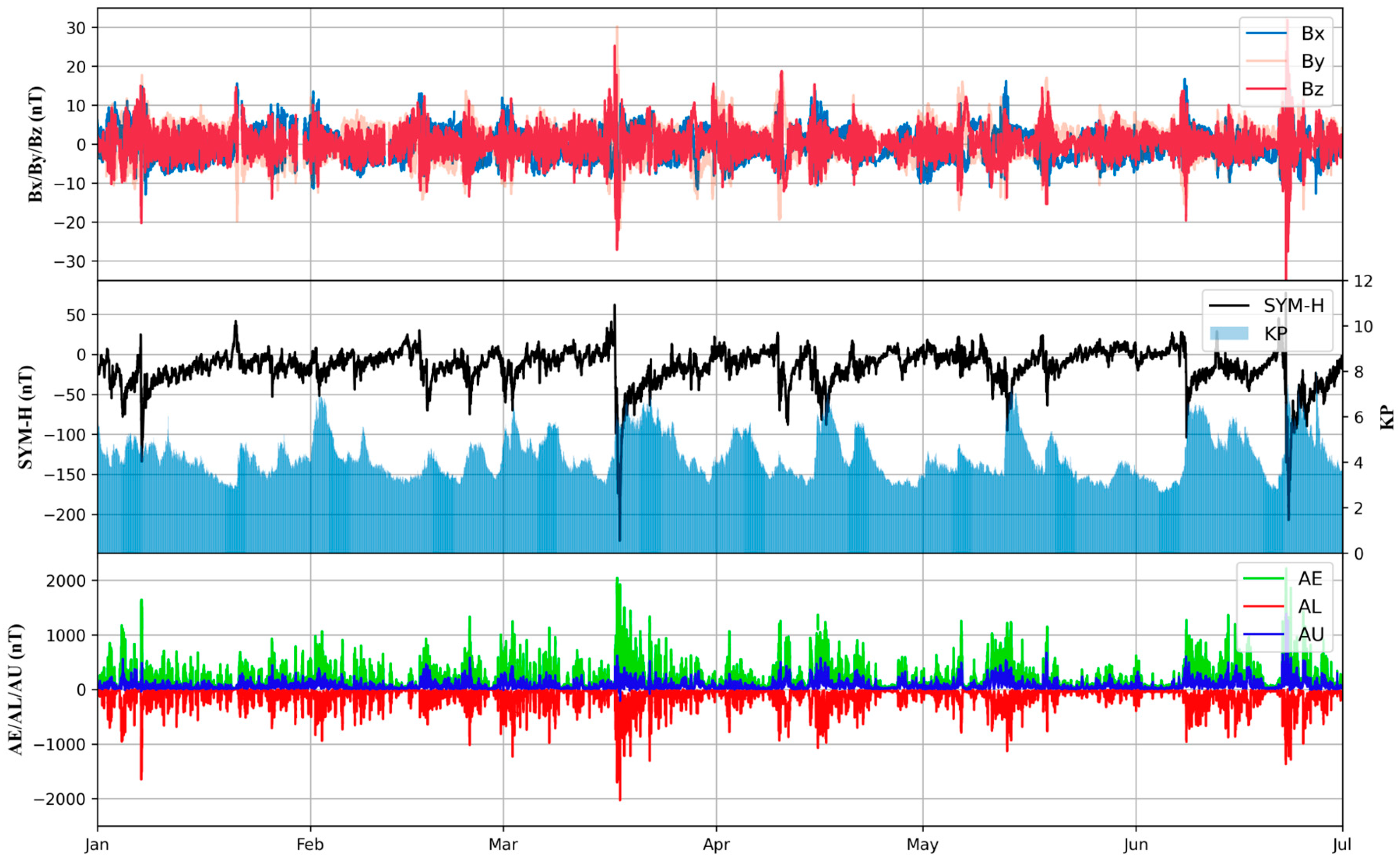
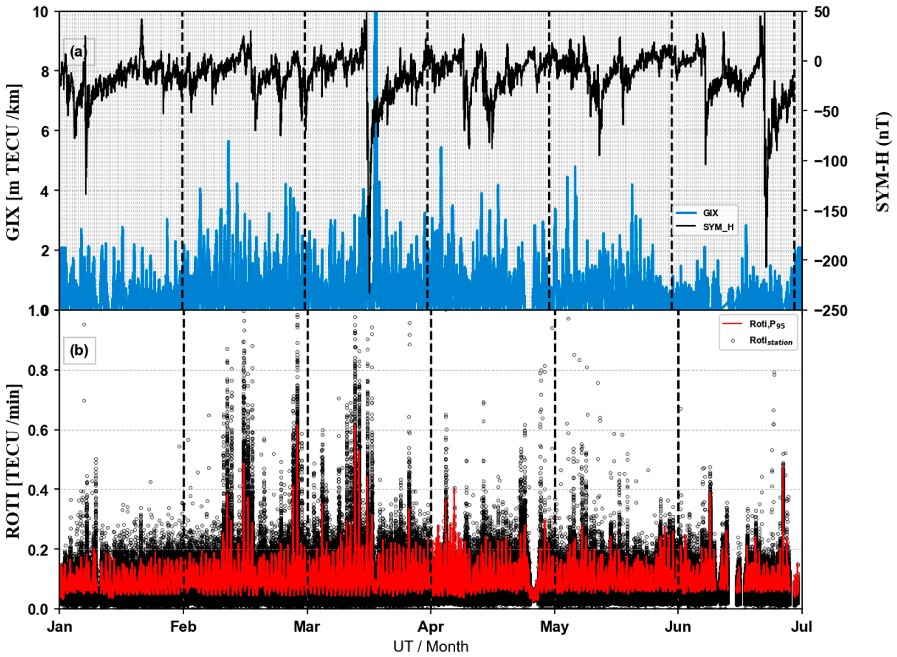
3.1. Overview of Geomagnetic Storm Periods and Ionospheric TEC Gradients Between 1 January and 30 June 2015

Between 1 January and 30 June 2015, geomagnetic and interplanetary conditions were comprehensively analyzed using data from NASA’s Solar Wind Data Lab via the OMNI dataset (https://cdaweb.gsfc.nasa.gov/). The analysis focused on the interplanetary magnetic field (IMF) components (Bx, By, Bz) and key geomagnetic indices, including SYM-H, AE, AL, AU, and Kp, as depicted in Figure 2.

In January and February, geomagnetic conditions remained relatively calm. The AE, AL, and AU indices exhibited occasional minor spikes, indicating low to moderate auroral activity, while the SYM-H index remained stable with only slight deviations, reflecting a quiet geomagnetic environment. However, in March, significant changes were observed. On 17 March 2015, a sudden storm commencement (SSC) occurred at 04:45 UT, marked by substantial alterations in the IMF components and a sharp decline in the SYM-H index. This event initiated the main phase of the St. Patrick’s Day geomagnetic storm. During the main phase, the SYM-H index plummeted to −234 nT, and the auroral indices (AE and AL) surged above 2000 nT. Concurrently, the Kp index sharply increased, exceeding 6, signifying a severe geomagnetic storm that persisted through 19 March.

In June, geomagnetic activity increased again, though not as severely as in March. A significant disturbance was observed on 23 June 2015. On this day, a notable geomagnetic storm occurred: SYM-H fell below −200 nT (Figure 2, middle panel), confirming an intense event. Throughout the remainder of June, the Kp index periodically rose above 4, and there were moderate fluctuations in the auroral electrojet indices and the SYM-H index, suggesting a series of minor to moderate geomagnetic disturbances.

Further analysis of ionospheric TEC gradient variations between 1 January and 30 June 2015 reveals distinct fluctuations in the GIX, ROTI, and SYM-H indices, as depicted in Figure 3. The GIX (blue line) and SYM-H (black line) indices illustrate variations in the averaged VTEC gradients and the symmetrical ring current index, respectively, highlighting peak activity during the 17 March storm. The ROTI values, represented by black dots, demonstrate variability in both spatial and temporal gradients of TEC across various GNSS stations. The red line, ROTI,P95, highlights periods of heightened ionospheric irregularities.

Notably, during the 2015 St. Patrick’s Day geomagnetic storm, the GIX reached its highest level, exceeding 10 mTECU/km. In contrast, the June geomagnetic storm did not produce a comparable increase in GIX, despite similar SYM-H disturbances. Additionally, ROTI exhibited several peaks aligned closely with GIX peaks, although ROTI did not show as pronounced an increase during the St. Patrick’s Day storm as GIX. Nevertheless, the markedly higher number of GNSS stations recording ROTI values greater than 0.4 TECU/min during this storm period compared to other intervals indicates substantial ionospheric disturbances. Combining the observations from Figure 2—which details geomagnetic and interplanetary conditions—with those from GIX and ROTI, our observations suggest that a strong geomagnetic storm event in March 2015 significantly impacted ionospheric conditions.

To further characterize the temporal behavior of ionospheric disturbances observed in these indices, we analyzed their diurnal variations, focusing specifically on gradients in four geographic directions across a 24 h cycle. Figure 4 illustrates these diurnal variations, averaged over the entire six-month period. The GIX index exhibited diurnal variation patterns. Specifically, the longitudinal VTEC spatial gradient, |GIXx,P95|, increased sharply during the morning hours from 00:00 to 08:00 UT (08:00–16:00 local time), peaking at approximately 50 mTECU/km around 12:00 UT. This pattern reflects heightened ionospheric activity associated with solar radiation effects during the local daytime. Subsequently, |GIXx,P95| rapidly declined between 12:00 and 16:00 UT (20:00–24:00 local time), consistent with decreasing solar illumination. In contrast, the latitudinal VTEC spatial gradient, GIXy,P95, exhibited minimal variability, maintaining a stable pattern throughout the day. Similarly, ROTI,P95 showed no pronounced diurnal changes, with values consistently remaining below 0.2 TECU/min throughout the 24 h cycle.

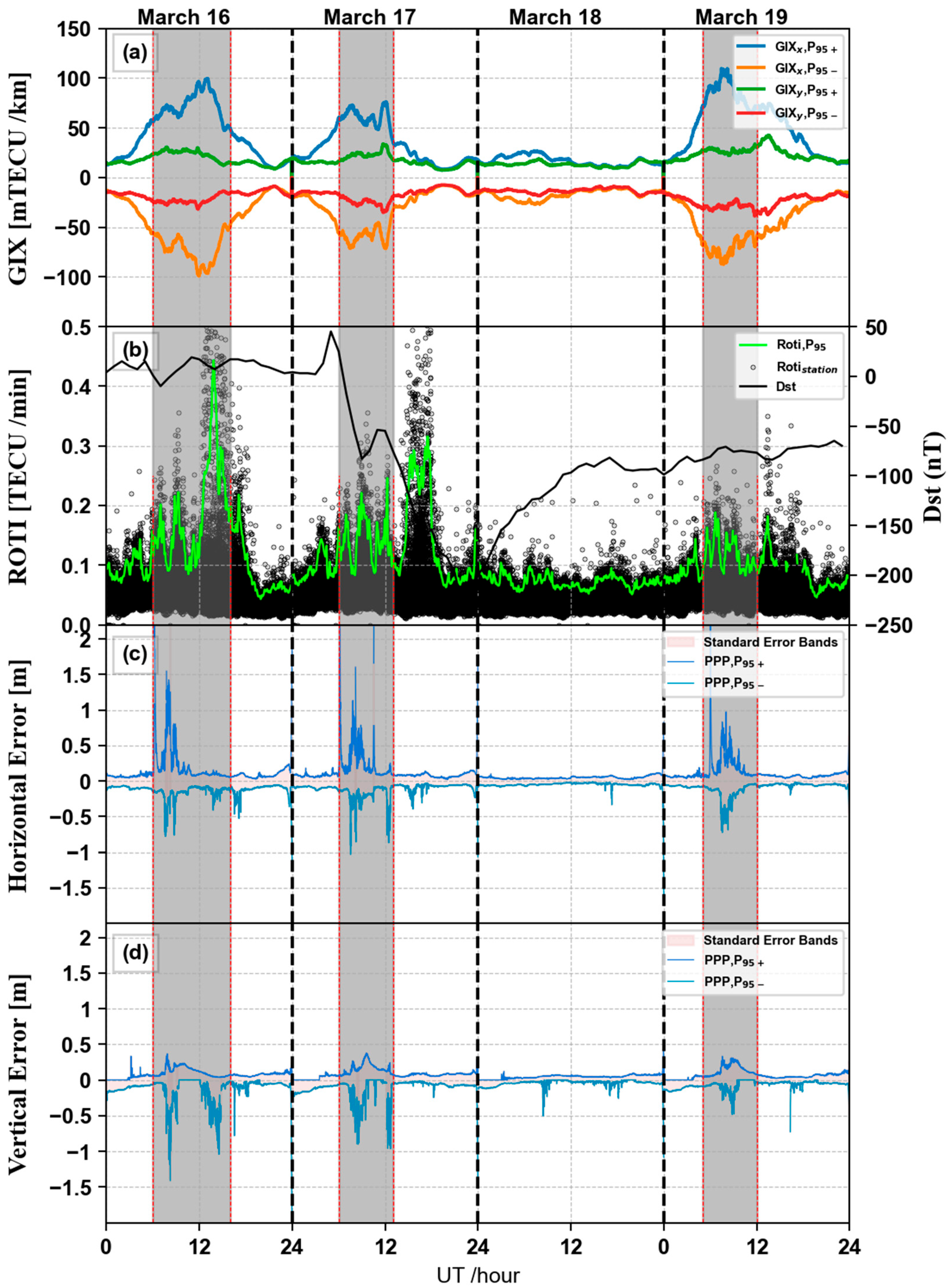
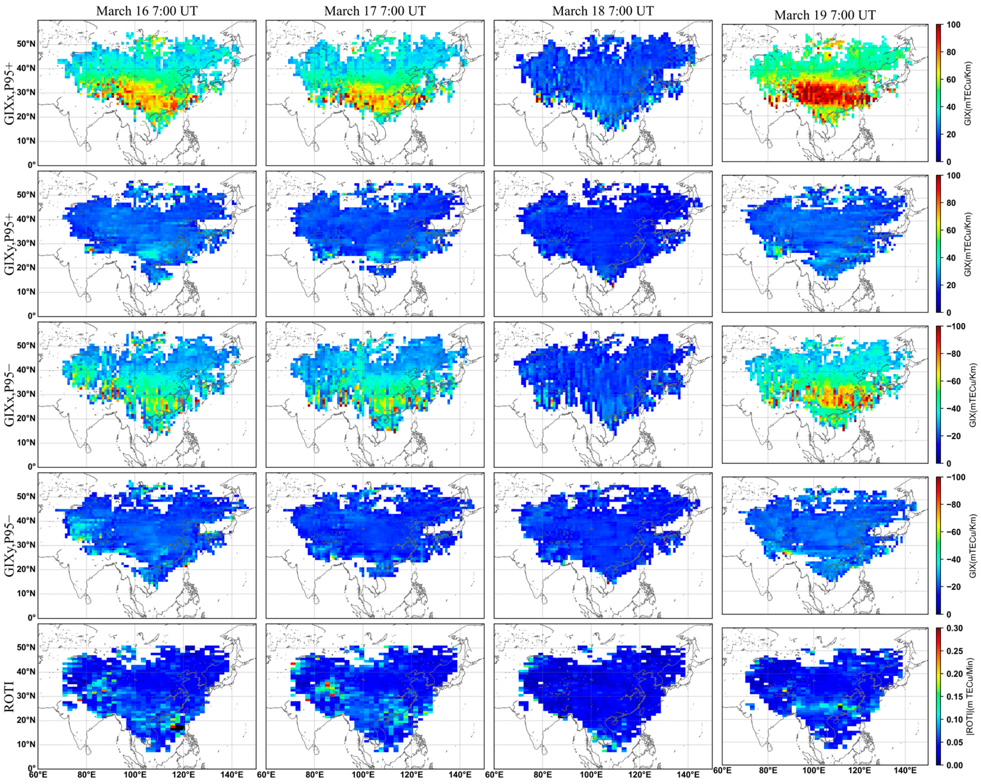
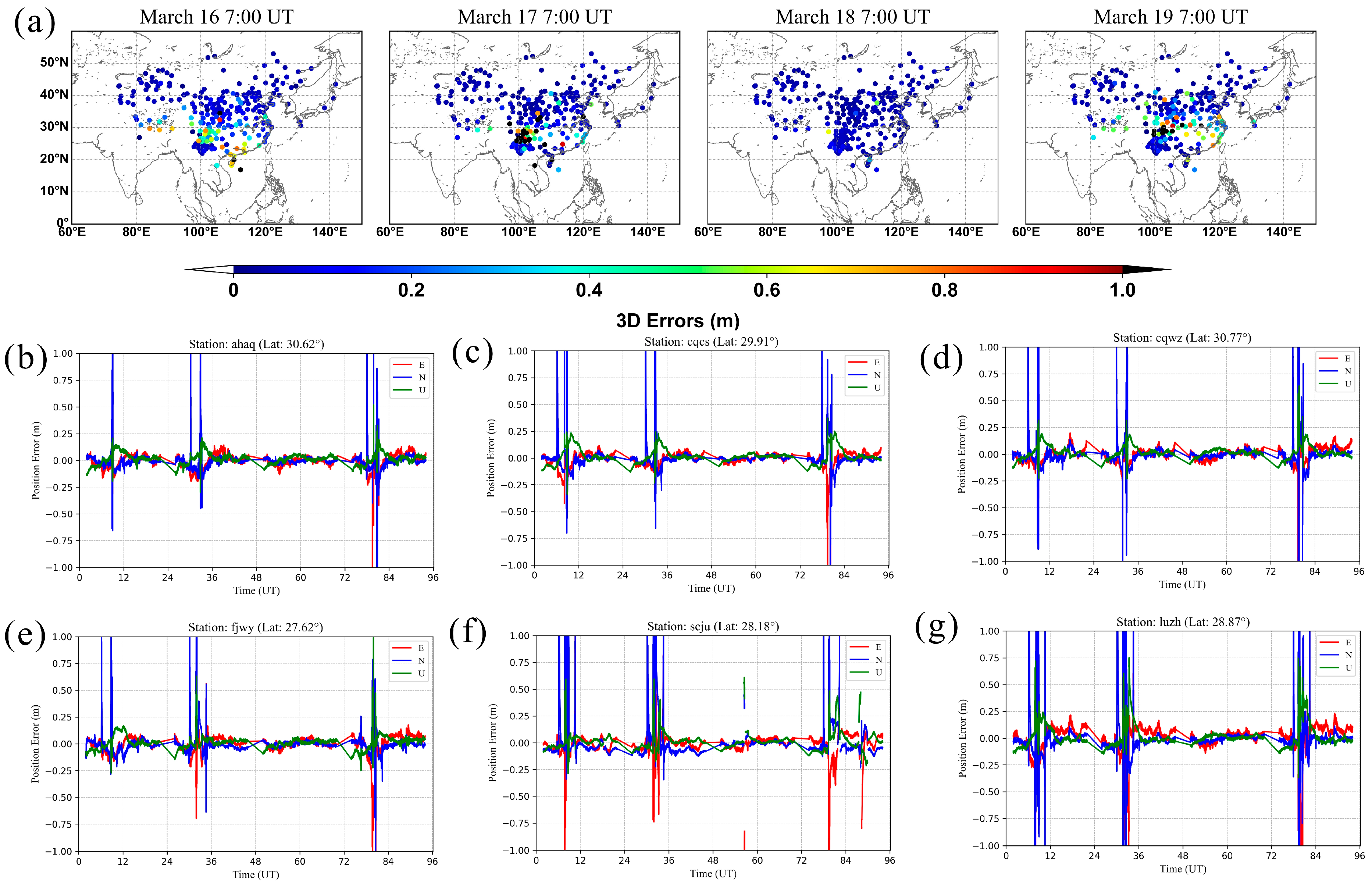
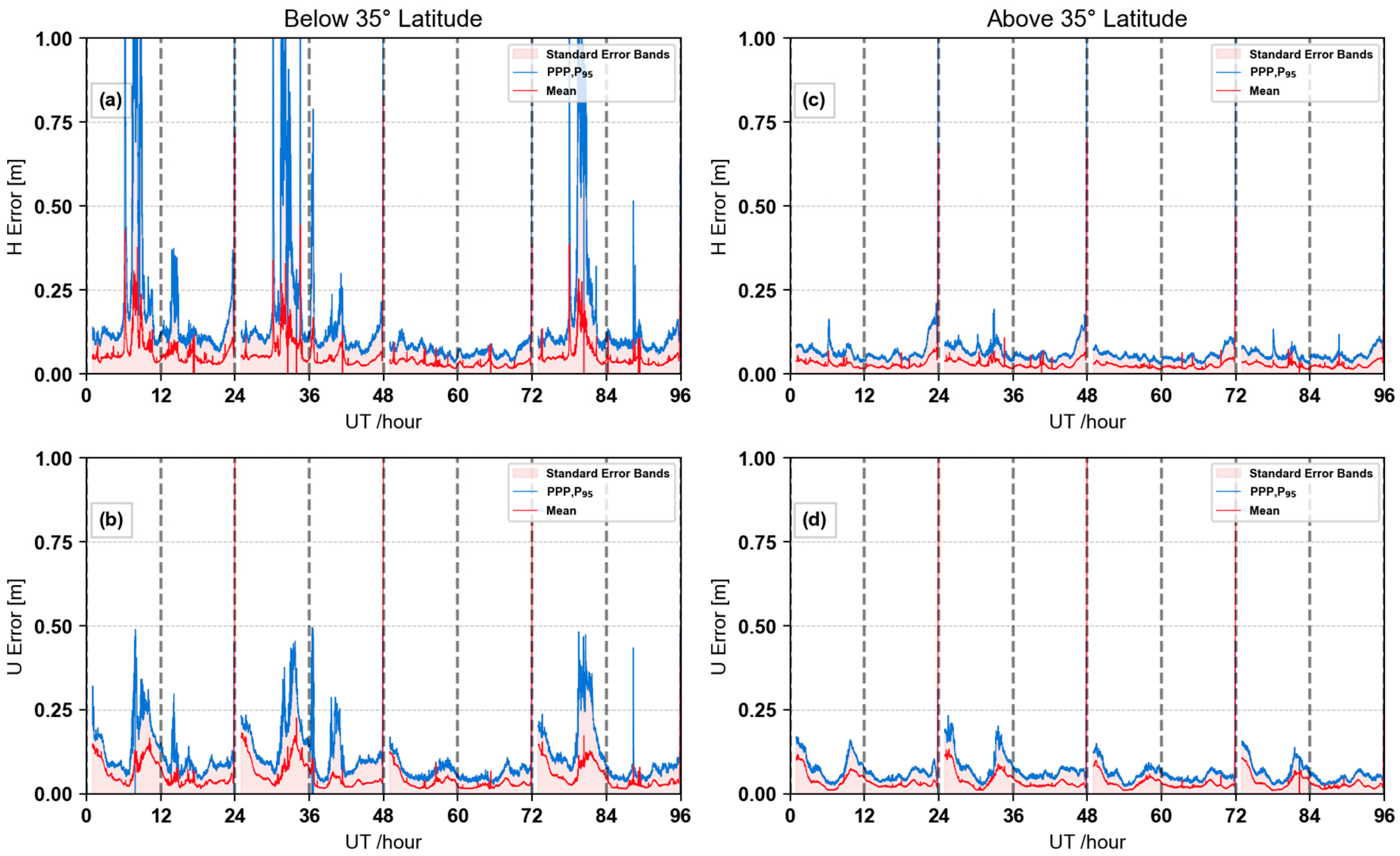
3.2. TEC Spatial Gradient and GNSS Positioning During the March 2015 Storm

Building upon the initial observations, we selected the March 2015 geomagnetic storm as a case study to analyze the temporal and spatial characteristics of geomagnetic storm impacts on the ionosphere in China, with a particular focus on the GIX and ROTI indices. The St. Patrick’s Day storm on 17 March 2015 was a severe geomagnetic event during solar cycle 24, providing an excellent opportunity to study ionospheric gradient variations under intense geomagnetic conditions.

Figure 5 illustrates the temporal evolution of selected ionospheric disturbance indices (GIX and ROTI) and the kinematic PPP solutions in 16–19 March 2015, over the China region. Based on the diurnal variations in GIX observed in Figure 4, a threshold of approximately 50 mTECU/km was used to differentiate between background ionospheric conditions and significant irregularities. It is noteworthy that large east–west TEC gradients (|GIXx,P95| > 50 mTECU/km) consistently correspond to substantial PPP errors during the storm period. Furthermore, the evolution of ionospheric irregularities, as indicated by each index, displayed distinct characteristics at different times during the storm.

Initial ionospheric disturbances were observed during the pre-storm period. On 16 March between 06:00 and 16:00 UT, GIX and ROTI both indicated notable increases in ionospheric irregularities (|GIXx,P95| > 50 mTECU/km and ROTI > 0.4 TECU/min). Concurrently, GNSS performance notably degraded, with horizontal and vertical PPP, P95 errors exceeding ±0.5 m; however, the peak in PPP degradation appeared earlier than the peak in ROTI.

During the storm’s main phase (17 March 06:00–23:00 UT), ROTI observations (Figure 5b) showed ionospheric irregularities (ROTI > 0.4 TECU/min) occurring later than those identified by GIX (which peaked between 06:00 and 13:00 UT). Specifically, between 06:00 and 13:00 UT on 17 March, strong VTEC spatial gradients (|GIXx,P95| > 50 mTECU/km) coincided closely with large PPP errors (>0.5 m). ROTI intensities increased subsequently, but the strongest PPP errors aligned directly with the peak values of |GIXx,P95|. After the storm entered its recovery phase at 23:06 UT on 17 March, two distinct ionospheric conditions emerged. On 18 March, during the recovery phase, both GIX and ROTI showed reduced irregularities (|GIXx,P95| < 35 mTECU/km and ROTI < 0.4 TECU/min), corresponding to improved PPP performance, with errors remaining within ±0.2 m. However, during the late recovery phase on 19 March (04:00–14:00 UT), intensified ionospheric irregularities reappeared, as indicated by elevated GIX values (|GIXx,P95| > 50 mTECU/km). This was accompanied by large positioning errors reemerging in the PPP solutions. Conversely, ROTI values remained consistently below 0.4 TECU/min, indicating a divergence between the two indices during this period.

Figure 6 further illustrates the spatial distribution of ionospheric TEC gradients, consistent with the temporal results shown in Figure 5. The horizontal gradient of VTEC is approximately twice as large in the geographic east–west direction (GIXx,P95+, GIXx,P95−) compared to the north–south direction (GIXy,P95+, GIXy,P95−). No significant spatial gradients (|GIXx,P95| and |GIXy,P95| < 40 mTECU/km) were evident at 07:00 UT on 18 March during the recovery phase. In contrast, on other days (16, 17, and 19 March at 07:00 UT), pronounced spatial gradients—particularly in the east–west direction (GIXx,P95+ > 60 mTECU/km)—were concentrated within the 20–35°N latitude region. Additionally, at 07:00 UT on 19 March, spatial gradients peaked significantly, exceeding 80 mTECU/km in the east–west direction (GIXx,P95+, GIXx,P95−). Although the ROTI results did not display the same clear band-like distribution as GIX, it is notable that ROTI values remained below 0.05 TECU/min across the region at 07:00 UT on 18 March. In contrast, during periods of enhanced horizontal spatial gradients—particularly on 16, 17, and 19 March—some regions exhibited ROTI values exceeding 0.15 TECU/min, primarily within the 20–35°N latitude band. These observations suggest that ionospheric irregularities were predominantly concentrated along this mid-to-low-latitude region.

Figure 7 presents snapshots of 1 h 3D kinematic PPP errors from 16 to 19 March 2015. From the spatial distribution of GNSS station PPP errors in Figure 7a, notable pre-storm enhancements were observed on 16 and 17 March, followed by a reduction in errors on 18 March and a significant increase again on 19 March. Further analysis of the east, north, and up components of PPP errors at selected low-latitude stations (Figure 7b–g) reveals that error magnitudes increased considerably when |GIXx,P95| exceeded 50 mTECU/km, as also indicated in Figure 5. Additionally, 3D PPP errors across GNSS stations located between 20°N and 35°N showed a clear increase (3D PPP, P₉₅ errors > 0.4 m), with maximum values exceeding 1 m. When combined with the results from Figure 6, it is evident that this alignment was particularly pronounced at 07:00 UT on March 19, when stations with large PPP errors corresponded spatially with regions where GIXx,P95+ exceeded 60 mTECU/km.

Figure 8a,b further illustrate the temporal evolution of PPP errors at different latitudes. The average horizontal positioning errors and PPP, P₉₅ errors for stations below 35°N increased from less than 0.1 m to over 0.25 m, and from approximately 0.1 m to more than 1 m, respectively. These increases were most significant on 16, 17, and 19 March, aligning with the spatial intensification of ionospheric TEC gradients (Figure 6) and the rise in 1 h 3D kinematic PPP, P₉₅ errors (Figure 7). In contrast, Figure 8c,d show that GNSS stations above 35°N maintained average and P95 horizontal positioning errors below 0.25 m throughout the period. This suggests that GNSS stations with noticeable PPP errors (3D PPP, P₉₅ errors > 0.4 m) closely corresponded to geographical regions experiencing intense ionospheric irregularities, where significant spatial gradient changes predominantly occurred within the 20–35°N latitude band.

4. Discussion

The severe St. Patrick’s Day geomagnetic storm (17 March 2015) occurred during solar cycle 24. Previous studies have documented the substantial impacts of geomagnetic storms on ionospheric stability, subsequently affecting GNSS positioning accuracy [22,23]. Numerous investigations have also explored the mechanisms underlying ionospheric disturbances and their effects on GNSS performance during storm events. In this study, we analyzed the temporal and spatial variations in PPP accuracy during the March 2015 storm. The evolution of ionospheric irregularities and PPP errors showed distinct temporal behavior, including a notable pre-storm enhancement. We also found that enhanced TEC gradients and larger GNSS positioning errors were concentrated within the 20–35°N latitude band. These pre-storm enhancements are evident in Figure 5, where notable increases in horizontal and vertical PPP errors coincide with intensified ionospheric irregularities during the pre-storm period (16 March). These findings are consistent with results in [35], which observed similar irregularities through phase scintillation and ROTI indices on 16 March. Additionally, the observed TEC enhancements during the pre-storm phase are consistent with previous studies [33,36,37]. Ondede et al. [38] further argued that ionospheric irregularities are not solely triggered by geomagnetic storms but can also arise from other factors. Considering the prevailing interplanetary and geomagnetic conditions, the enhanced TEC gradients observed in the pre-storm phase were likely related to zonal electric fields.

Following the onset of the main storm phase at 06:00 UT on 17 March, increased geomagnetic activity produced various ionospheric disturbances. Kuai et al. [39] reported that irregularities observed on 17 March were largely influenced by east–west penetration electric fields (PEFs), associated with a sudden southward turning of IMF Bz during daytime hours. Interestingly, during the main storm phase (06:00–23:00 UT, 17 March), ROTI-indicated irregularities (>0.4 TECU/min) appeared later than those indicated by GIX (06:00–13:00 UT).

During the recovery phase, starting at 23:06 UT on 17 March, two distinct ionospheric conditions emerged. Prior research suggests that geomagnetic storms can either generate or inhibit ionospheric scintillation [40,41,42]. Fuller-Rowell [43] proposed that storms might both suppress and enhance irregularities, a view further supported by recent findings [44]. On 18 March, the observed reduction in TEC gradients, ROTI, and PPP errors can be explained by ionospheric electrodynamics; specifically, Polekh et al. [45] and Sun [46] suggest that strong westward disturbance dynamo electric fields (DDEFs) significantly suppressed equatorial spread-F (ESF) and associated scintillation, resulting in reduced ionospheric disturbances.

However, intensified irregularities reappeared during the late recovery phase on 19 March, coinciding with large GNSS positioning errors. These observations align with previous studies examining changes in DTEC and TEC [39,46,47]. Specifically, Kuai et al. [39] reported that intensified daytime eastward electric fields on 19 March increased TEC within the EIA regions. Additionally, Sun et al. [46] provided evidence of ionospheric scintillation events occurring simultaneously in low-latitude China based on ionospheric F2-layer critical frequency (f₀F₂) measurements.

Figure 6, Figure 7 and Figure 8 confirm that enhanced TEC gradients and larger GNSS positioning errors were confined to 20–35°N. This storm was primarily driven by PEFs and DDEFs, both of which exhibited significant local-time dependence and played crucial roles in the observed ionospheric effects at low latitudes in East Asia [39,45]. Polekh et al. [45] and Liu et al. [48] suggested that the considerable disparity between geographic and geomagnetic latitudes in East Asia leads to variations in disturbance mechanisms and dynamic characteristics at different latitudes. Specifically, during the St. Patrick’s Day geomagnetic storm, PEFs and DDEFs were two dominant sources of electric fields strongly influencing ionospheric responses at low latitudes [35]. These electric fields likely contributed to the enhanced spatial gradients and the corresponding GNSS positioning errors concentrated within the 20–35°N latitude region.

Additionally, the analysis revealed that intervals when the |GIXx,P95| index exceeded 50 mTECU/km coincided closely with periods of significant GNSS positioning errors in PPP solutions. This alignment supports the effectiveness of GIX as a reliable indicator of ionospheric disturbances, thereby aiding efforts to reduce safety and accuracy risks in GNSS navigation and positioning.

5. Conclusions

Using data from approximately 260 GNSS stations across China, this study investigated the impact of geomagnetic storms on ionospheric disturbances between 1 January and 30 June 2015. Interplanetary parameters and geomagnetic storm indices, together with the ionospheric disturbance indices GIX and ROTI, clearly identified the major March 2015 event (the St Patrick’s Day storm) and its pronounced effect on ionospheric spatial gradients. Detailed temporal–spatial analysis showed that large east–west TEC gradients (|GIXx,P95| > 50 mTECU/km) were consistently associated with substantial PPP errors throughout the storm. These strong gradients were chiefly confined to the mid-to-low-latitude belt between 20° and 35°N, where significant 3D PPP errors (PPP, P₉₅ > 0.4 m) were likewise concentrated, confirming the direct link between intense ionospheric gradients and GNSS positioning degradation.

Our results also revealed notable pre-storm enhancements on 16 March and contrasting behaviors during the two recovery-phase days, 18 and 19 March. The pre-storm irregularities were likely driven by zonal electric fields associated with the prevailing interplanetary and geomagnetic conditions. By 18 March, strong westward DDEFs appeared to suppress ESF and scintillation, leading to weaker ionospheric disturbances and improved PPP accuracy. In contrast, intensified irregularities returned on 19 March, most likely triggered by daytime PEFs that enhanced TEC within the EIA and sharply degraded PPP performance. Together, these findings imply that GIX not only quantifies spatial gradient anomalies but also helps to elucidate the underlying electrodynamic drivers of ionospheric disturbances. Continuous monitoring of horizontal ionospheric gradients with indices such as GIX therefore provides a reliable means to anticipate ionospheric threats and to safeguard GNSS positioning accuracy and reliability during geomagnetic storm events.

References

1. Kung Chie, Y.; Chao-Han, L. Radio wave scintillations in the ionosphere. Proc. IEEE 1982, 70, 324–360. [Google Scholar] [CrossRef]
2. Kintner, P.M.; Ledvina, B.M.; De Paula, E.R. GPS and ionospheric scintillations. Space Weather 2007, 5, 2006SW000260. [Google Scholar] [CrossRef]
3. DasGupta, A.; Ray, S.; Paul, A.; Banerjee, P.; Bose, A. Errors in position-fixing by GPS in an environment of strong equatorial scintillations in the Indian zone. Radio Sci. 2004, 39, 2002RS002822. [Google Scholar] [CrossRef]
4. Jacobsen, K.S.; Dähnn, M. Statistics of ionospheric disturbances and their correlation with GNSS positioning errors at high latitudes. J. Space Weather Space Clim. 2014, 4, A27. [Google Scholar] [CrossRef]
5. Dugassa, T.; Bosco Habarulema, J.; Nigussie, M. Investigation of the relationship between the spatial gradient of total electron content (TEC) between two nearby stations and the occurrence of ionospheric irregularities. Ann. Geophys. 2019, 37, 1161–1180. [Google Scholar] [CrossRef]
6. Jakowski, N.; Stankov, S.M.; Klaehn, D. Operational space weather service for GNSS precise positioning. Ann. Geophys. 2005, 23, 3071–3079. [Google Scholar] [CrossRef]
7. Nava, B.; Radicella, S.M.; Leitinger, R.; Coïsson, P. Use of total electron content data to analyze ionosphere electron density gradients. Adv. Space Res. 2007, 39, 1292–1297. [Google Scholar] [CrossRef]
8. Lee, J.; Datta-Barua, S.; Zhang, G.; Pullen, S.; Enge, P. Observations of low-elevation ionospheric anomalies for ground-based augmentation of GNSS. Radio Sci. 2011, 46, RS6005. [Google Scholar] [CrossRef]
9. Vukovic, J.; Kos, T. Ionospheric spatial and temporal gradients for disturbance characterization. In Proceedings of the 2016 European Navigation Conference (ENC), Helsinki, Finland, 30 May–2 June 2016; pp. 1–4. [Google Scholar] [CrossRef]
10. Pi, X.; Mannucci, A.J.; Lindqwister, U.J.; Ho, C.M. Monitoring of global ionospheric irregularities using the Worldwide GPS Network. Geophys. Res. Lett. 1997, 24, 2283–2286. [Google Scholar] [CrossRef]
11. Jakowski, N.; Hoque, M.M. Estimation of Spatial Gradients and Temporal Variations of the Total Electron Content Using Ground-Based GNSS Measurements. Space Weather 2019, 17, 339–356. [Google Scholar] [CrossRef]
12. Cesaroni, C.; Spogli, L.; Alfonsi, L.; De Franceschi, G.; Ciraolo, L.; Galera Monico, J.F.; Scotto, C.; Romano, V.; Aquino, M.; Bougard, B. L-band scintillations and calibrated total electron content gradients over Brazil during the last solar maximum. J. Space Weather Space Clim. 2015, 5, A36. [Google Scholar] [CrossRef]
13. Beach, T.L.; Kintner, P.M. Simultaneous Global Positioning System observations of equatorial scintillations and total electron content fluctuations. J. Geophys. Res. Space Phys. 1999, 104, 22553–22565. [Google Scholar] [CrossRef]
14. Bhattacharyya, A.; Beach, T.L.; Basu, S.; Kintner, P.M. Nighttime equatorial ionosphere: GPS scintillations and differential carrier phase fluctuations. Radio Sci. 2000, 35, 209–224. [Google Scholar] [CrossRef]
15. Sun, Y.Y.; Matsuo, T.; Araujo-Pradere, E.A.; Liu, J.Y. Ground-based GPS observation of SED-associated irregularities over CONUS. J. Geophys. Res. Space Phys. 2013, 118, 2478–2489. [Google Scholar] [CrossRef]
16. Aa, E.; Zhang, S.R.; Erickson, P.J.; Wang, W.; Qian, L.; Cai, X.; Coster, A.J.; Goncharenko, L.P. Significant Mid- and Low-Latitude Ionospheric Disturbances Characterized by Dynamic EIA, EPBs, and SED Variations During the 13–14 March 2022 Geomagnetic Storm. J. Geophys. Res. Space Phys. 2023, 128, e2023JA031375. [Google Scholar] [CrossRef]
17. Vo, H.B.; Foster, J.C. A quantitative study of ionospheric density gradients at midlatitudes. J. Geophys. Res. Space Phys. 2001, 106, 21555–21563. [Google Scholar] [CrossRef]
18. Klimenko, M.V.; Zakharenkova, I.E.; Klimenko, V.V.; Lukianova, R.Y.; Cherniak, I.V. Simulation and Observations of the Polar Tongue of Ionization at Different Heights During the 2015 St. Patrick’s Day Storms. Space Weather 2019, 17, 1073–1089. [Google Scholar] [CrossRef]
19. Zhang, Y.; Liu, Y.; Mei, J.; Zhang, C.; Wang, J. A Study on the Characteristics of the Ionospheric Gradient under Geomagnetic Perturbations. Sensors 2020, 20, 1805. [Google Scholar] [CrossRef]
20. Cherniak, I.V.; Zakharenkova, I. High-latitude ionospheric irregularities: Differences between ground- and space-based GPS measurements during the 2015 St. Patrick’s Day storm. Earth Planets Space 2016, 68, 136. [Google Scholar] [CrossRef]
21. Liu, Q.; Hernández-Pajares, M.; Yang, H.; Monte-Moreno, E.; García-Rigo, A.; Lyu, H.; Olivares-Pulido, G.; Orús-Pérez, R. A New Way of Estimating the Spatial and Temporal Components of the Vertical Total Electron Content Gradient Based on UPC-IonSAT Global Ionosphere Maps. Space Weather 2022, 20, e2021SW002926. [Google Scholar] [CrossRef]
22. Cherniak, I.; Zakharenkova, I. Dependence of the high-latitude plasma irregularities on the auroral activity indices: A case study of 17 March 2015 geomagnetic storm. Earth Planets Space 2015, 67, 151. [Google Scholar] [CrossRef]
23. Jacobsen, K.S.; Andalsvik, Y.L. Overview of the 2015 St. Patrick’s day storm and its consequences for RTK and PPP positioning in Norway. J. Space Weather Space Clim. 2016, 6, A9. [Google Scholar] [CrossRef]
24. Yang, Z.; Morton, Y.T.J.; Zakharenkova, I.; Cherniak, I.; Song, S.; Li, W. Global View of Ionospheric Disturbance Impacts on Kinematic GPS Positioning Solutions During the 2015 St. Patrick’s Day Storm. J. Geophys. Res. Space Phys. 2020, 125, e2019JA027681. [Google Scholar] [CrossRef]
25. Ma, G.; Li, Q.; Li, J.; Wan, Q.; Fan, J.; Wang, X.; Maruyama, T.; Zhang, J. A study of ionospheric irregularities with spatial fluctuation of TEC. J. Atmos. Sol.-Terr. Phys. 2020, 211, 105485. [Google Scholar] [CrossRef]
26. Li, Z.; Yuan, Y.; Fan, L.; Huo, X.; Hsu, H. Determination of the Differential Code Bias for Current BDS Satellites. IEEE Trans. Geosci. Remote Sens. 2014, 52, 3968–3979. [Google Scholar] [CrossRef]
27. Wang, N.; Yuan, Y.; Li, Z.; Montenbruck, O.; Tan, B. Determination of differential code biases with multi-GNSS observations. J. Geod. 2016, 90, 209–228. [Google Scholar] [CrossRef]
28. Li, Z.; Yuan, Y.; Li, H.; Ou, J.; Huo, X. Two-step method for the determination of the differential code biases of COMPASS satellites. J. Geod. 2012, 86, 1059–1076. [Google Scholar] [CrossRef]
29. Li, W.; Li, Z.; Wang, N.; Liu, A.; Zhou, K.; Yuan, H.; Krankowski, A. A satellite-based method for modeling ionospheric slant TEC from GNSS observations: Algorithm and validation. GPS Solut. 2022, 26, 14. [Google Scholar] [CrossRef]
30. Takasu, T.; Yasuda, A. Development of the low-cost RTK-GPS receiver with an open source program package RTKLIB. In Proceedings of the International Symposium on GPS/GNSS, JeJu, Republic of Korea, 4–9 November 2009; Volume 1, pp. 1–6. [Google Scholar]
31. Hoque, M.M.; Jakowski, N.; Berdermann, J. A New Approach for Ionospheric TEC Prediction at a GPS Station. In Proceedings of the 29th International Technical Meeting of the Satellite Division of The Institute of Navigation (ION GNSS+ 2016), Portland, OR, USA, 12–16 September 2016; pp. 1649–1656. [Google Scholar] [CrossRef]
32. Nguyen, C.T.; Oluwadare, S.T.; Le, N.T.; Alizadeh, M.; Wickert, J.; Schuh, H. Spatial and Temporal Distributions of Ionospheric Irregularities Derived from Regional and Global ROTI Maps. Remote Sens. 2021, 14, 10. [Google Scholar] [CrossRef]
33. Liu, J.; Liu, L.; Zhao, B.; Wei, Y.; Hu, L.; Xiong, B. High-speed stream impacts on the equatorial ionization anomaly region during the deep solar minimum year 2008. J. Geophys. Res. Space Phys. 2012, 117, 2012JA018015. [Google Scholar] [CrossRef]
34. Gao, H.Y.; Zhang, D.H.; Liu, Z.Z.; Sun, S.J.; Hao, Y.Q.; Xiao, Z. Revisiting the Variation of the Ionospheric Irregularities in the Low Latitude Region of China Based on Small Regional Geodetic GNSS Station Network. Space Weather 2023, 21, e2023SW003452. [Google Scholar] [CrossRef]
35. Nie, W.; Rovira-Garcia, A.; Li, M.; Fang, Z.; Wang, Y.; Zheng, D.; Xu, T. The Mechanism for GNSS-Based Kinematic Positioning Degradation at High-Latitudes Under the March 2015 Great Storm. Space Weather 2022, 20, e2022SW003132. [Google Scholar] [CrossRef]
36. Kutiev, I.; Otsuka, Y.; Saito, A.; Watanabe, S. GPS observations of post-storm TEC enhancements at low latitudes. Earth Planets Space 2006, 58, 1479–1486. [Google Scholar] [CrossRef]
37. Kutiev, I.; Otsuka, Y.; Saito, A.; Tsugawa, T. Low-latitude total electron content enhancement at low geomagnetic activity observed over Japan. J. Geophys. Res. Space Phys. 2007, 112, A07306. [Google Scholar] [CrossRef]
38. Ondede, G.O.; Rabiu, A.B.; Okoh, D.; Baki, P.; Olwendo, J.; Shiokawa, K.; Otsuka, Y. Relationship between geomagnetic storms and occurrence of ionospheric irregularities in the west sector of Africa during the peak of the 24th solar cycle. Front. Astron. Space Sci. 2022, 9, 969235. [Google Scholar] [CrossRef]
39. Kuai, J.; Liu, L.; Liu, J.; Sripathi, S.; Zhao, B.; Chen, Y.; Le, H.; Hu, L. Effects of disturbed electric fields in the low-latitude and equatorial ionosphere during the 2015 St. Patrick’s Day storm. J. Geophys. Res. Space Phys. 2016, 121, 9111–9126. [Google Scholar] [CrossRef]
40. Aarons, J. The role of the ring current in the generation or inhibition of equatorial F layer irregularities during magnetic storms. Radio Sci. 1991, 26, 1131–1149. [Google Scholar] [CrossRef]
41. Kassa, T.; Damtie, B. Ionospheric irregularities over Bahir Dar, Ethiopia during selected geomagnetic storms. Adv. Space Res. 2017, 60, 121–129. [Google Scholar] [CrossRef]
42. Li, G.; Ning, B.; Zhao, B.; Liu, L.; Liu, J.Y.; Yumoto, K. Effects of geomagnetic storm on GPS ionospheric scintillations at Sanya. J. Atmos. Sol.-Terr. Phys. 2008, 70, 1034–1045. [Google Scholar] [CrossRef]
43. Fuller-Rowell, T.J. The “thermospheric spoon”: A mechanism for the semiannual density variation. J. Geophys. Res. Space Phys. 1998, 103, 3951–3956. [Google Scholar] [CrossRef]
44. Aol, S.; Habyarimana, V.; Mungufeni, P.; Buchert, S.C.; Habarulema, J.B. Ground and Space-based response of the ionosphere during the geomagnetic storm of 02–06 November 2021 over the low-latitudes across different longitudes. Adv. Space Res. 2024, 73, 3014–3032. [Google Scholar] [CrossRef]
45. Polekh, N.; Zolotukhina, N.; Kurkin, V.; Zherebtsov, G.; Shi, J.; Wang, G.; Wang, Z. Dynamics of ionospheric disturbances during the 17–19 March 2015 geomagnetic storm over East Asia. Adv. Space Res. 2017, 60, 2464–2476. [Google Scholar] [CrossRef]
46. Sun, W.-J.; Ning, B.-Q.; Zhao, B.-Q.; Li, G.-Z.; Hu, L.-H.; Chang, S.-M. Analysis of ionospheric features in middle and low latitude region of China during the geomagnetic storm in March 2015. Chin. J. Geophys. 2017, 60, 1–10. Available online: http://www.geophy.cn//article/id/dqwlxb_13338 (accessed on 1 January 2017).
47. Nava, B.; Rodríguez-Zuluaga, J.; Alazo-Cuartas, K.; Kashcheyev, A.; Migoya-Orué, Y.; Radicella, S.M.; Amory-Mazaudier, C.; Fleury, R. Middle- and low-latitude ionosphere response to 2015 St. Patrick’s Day geomagnetic storm. J. Geophys. Res. Space Phys. 2016, 121, 3421–3438. [Google Scholar] [CrossRef]
48. Liu, J.; Zhang, D.-H.; Coster, A.J.; Zhang, S.-R.; Ma, G.-Y.; Hao, Y.-Q.; Xiao, Z. A case study of the large-scale traveling ionospheric disturbances in the eastern Asian sector during the 2015 St. Patrick’s Day geomagnetic storm. Ann. Geophys. 2019, 37, 673–687. [Google Scholar] [CrossRef]
Figure 1. Locations of the GNSS stations from different networks: CMONOC (yellow triangles) and IGS (blue dots) in this study.
Remotesensing 17 02027 g001
Figure 2. Variations in geomagnetic and interplanetary conditions from 1 January to 30 June 2015.
Remotesensing 17 02027 g002
Figure 3. Evolution of GIX and SYM-H indexes and ROTI variations from 1 January to 30 June 2015: (a) GIX (blue line) and SYM-H (black line) illustrate the variations in the averaged VTEC gradients and the symmetrical ring current index, respectively, highlighting the peak activities during the 17 March storm; (b) ROTI—with individual station values represented by black dots, and the average ROTI values at stations exceeding the 95th percentile (ROTI,P95) shown by the red line, demonstrating periods of heightened ionospheric irregularities. The GIX values represent the total components of the GIX index and are multiplied by 5 for a better comparison with the SYM-H index.
Remotesensing 17 02027 g003
Figure 4. Hourly averages of ionospheric disturbance indices over six months: (a) hourly averages of G I X x , P 95 + , G I X x , P 95 , G I X y , P 95 + , and G I X y , P 95 computed over the period from 1 January to 30 June 2015. Each day’s data is normalized to a 24 h cycle, and averages are calculated for each hour across the entire period to analyze diurnal variations; (b) hourly average of the ROTI, and P95 calculated in the same manner, reflecting periodic daily fluctuations throughout the six-month period.
Remotesensing 17 02027 g004
Figure 5. The evolution of (a) GIX (i.e., GIXx,P95+, GIXx,P95−, GIXy,P95+, and GIXy,P95−); (b) ROTI (i.e., ROTI,P95) and Dst; (c) horizontal error, and (d) vertical error of kinematic PPP solutions on 16–19 March 2015. The gray shaded area represents GIXx,P95+ > 50 mTECU/km. The shaded area in panels (c,d) represents the standard error bands of the PPP solution errors.
Remotesensing 17 02027 g005
Figure 6. Snapshots at 07:00 UT each day for the strong geomagnetic storm on 16–19 March 2015, showing 1 h interval changes in GIXx,P95+; GIXy,P95+; GIXx,P95−; GIXy,P95−; and ROTI.
Remotesensing 17 02027 g006
Figure 7. (a) Snapshots of 1 h 3D kinematic PPP, P95 errors on 16–19 March 2015, each at 07:00 UT. (bg) Errors of kinematic PPP solutions in 20–35° strip region on 16–19 March 2015.
Remotesensing 17 02027 g007
Figure 8. Horizontal (a,c) and vertical (b,d) errors of kinematic PPP solutions at different latitudes on 16–19 March 2015. (a,b) show PPP errors from 124 GNSS stations below 35°N latitude; (c,d) utilize data from 129 GNSS stations above 35°N latitude; “PPP, P95” represents the mean of PPP error values exceeding the 95th percentile of absolute error at the same time, while “Mean” indicates the average of all errors at that time; the shaded areas represent standard error bands.
Remotesensing 17 02027 g008