Assessing the Synergistic Use of Sentinel-1, Sentinel-2, and LiDAR Data for Forest Type and Species Classification

Abstract

The design of effective forest management strategies requires the precise characterization of forested areas. Currently, different remote sensing technologies can be used for forest mapping, with optical sensors being the most common. The objective of this study was to evaluate the synergistic use of Sentinel-1, Sentinel-2, and LiDAR data for classifying forest types and species. With this aim, a case study was conducted using random forest, considering three classification levels of increasing complexity. The classifications incorporated Sentinel-1 and Sentinel-2 monthly composites, along with LiDAR metrics and topographic variables. The results showed that the combination of Sentinel-2 monthly composites, LiDAR, and topographic variables obtained the highest overall accuracies (0.90 for level 1, 0.80 for level 2, and 0.79 for level 3). The most important variables were identified as Sentinel-2 red-edge and NIR bands from June, July, and August, along with height-related LiDAR and topographic variables. Although not as precise as Sentinel-2 at the species level, Sentinel-1 enabled the classification of broad forest types with remarkable accuracy (0.80), especially when combined with LiDAR data (0.83). Altogether, the results of this study demonstrate the potential of combining data from different Earth observation technologies to enhance the mapping of forest types and species.

1. Introduction

Forests play a vital role in sustaining the conditions for life on Earth [1]. They function as carbon sinks, regulate global climate patterns [2], and serve as key reservoirs of biodiversity [3]. Well-managed forests can provide a variety of economic resources, thereby sustaining local economies and livelihoods [4]. However, the global forest area has decreased by approximately 178 million hectares over the past three decades [5], mainly due to factors such as deforestation and climate change [6].

Achieving an accurate and up-to-date characterization of forests is essential for their effective management. Remote sensing (RS) plays a crucial role in this sense, with a diverse range of applications related to forest ecology [7] and management [8], such as forest inventory [9], wildfire mapping [10], or land-cover change monitoring [11]. Forest type and species mapping is of paramount importance for a range of environmental and management applications [12]. The most effective approach for this purpose is RS image classification.

Multi- and hyper-spectral imagery has been frequently employed to classify forest types and species. In recent years, there has been a specific emphasis on data from the Sentinel-2 (S-2) mission [13,14], as it provides high spatial, temporal, and spectral resolution data that is already processed and ready for use. The reflectance at the visible-infrared wavelengths is sensitive to vegetation biophysical properties, providing valuable information for classifying forest areas [15]. Vegetation indices such as the Normalized Burn Ratio (NBR) or the Enhanced Vegetation Index (EVI) have also been used as input in forest classification models [6,16]. However, it is important to note that the availability of images may be affected by persistent cloud cover in specific regions of the world.

Synthetic Aperture Radar (SAR) and Light Detection and Ranging (LiDAR) are active sensors that have also been used for forest classification, although not to the same extent as optical data. LiDAR is frequently employed for estimating biomass and structural parameters of forests [17,18]. Conversely, SAR sensors provide information about the dielectric and geometric characteristics of targets [19], which might also be related to biomass [20]. SAR data from the Sentinel-1 (S-1) mission has been used for various forest applications [21,22], mostly due to its availability, its high temporal resolution, and its ability to penetrate through clouds.

LiDAR sensors capture 3D point clouds of canopies, thereby enabling precise measurements of forest height, density, and biomass. Point clouds can provide numerous metrics, which can be categorized into geometric and radiometric metrics. The former can characterize structural attributes of trees, such as their height or crown shape, whereas the latter relates to the intensity and other parameters of the received echoes [23]. The potential of LiDAR features for forest classification has been demonstrated in several studies [24,25], although these features are often combined with data derived from other sensors [26,27].

There is a growing interest in the integration of Earth observation data obtained from different types of sensors for applications, including those related to forests [28]. A substantial body of research has examined the performance of classification approaches that integrate optical and radar data [29,30]. These studies typically conclude that the multi-sensor approach yields enhanced classification results when compared to individual approaches [31]. However, in some cases, the addition of S-1 data to S-2 did not result in substantial improvements [32]. On the other hand, the majority of studies that integrated LiDAR and optical or SAR data focused on the estimation of forest attributes such as height or biomass [33,34], rather than on the classification of forest types and species [35,36]. Nevertheless, the integration of the three data sources (i.e., optical, SAR, and LiDAR) for forest classification has not received sufficient attention.

Although the use of RS data for forest classification is well established, several gaps and challenges persist in this field. Few studies have assessed how multi-sensor integrations contribute to classification performance across increasing levels of complexity. The value of multi-sensor approaches has often been highlighted, although there is still a lack of systematic frameworks that quantify the relative contribution of each sensor type to forest classification accuracy, particularly when transitioning from general forest types to species-level classes. A key gap lies in the limited number of studies that address complex, ecologically meaningful forest classifications using operational RS data. Methodological challenges include dealing with class imbalances, optimizing feature selection across heterogeneous data sources, and scaling classification approaches while maintaining interpretability.

To address these limitations, this study presents a structured, comparative assessment of multi-sensor integration across multiple classification levels. Specifically, it evaluates the synergistic use of S-1, S-2, and LiDAR data for forest types and species classification. With this aim, a case study was conducted in the province of Navarre, Spain, which is characterized by a wide diversity of forest systems. Fourteen classification scenarios were evaluated, considering different combinations of input variables from the aforementioned sensors. Three classification levels of increasing complexity were considered: the first and the simplest level included three general forest types (broadleaves, conifers, and mixed); the second level comprised 11 forest classes; and the most detailed third level distinguished 22 distinct forest species. A comprehensive analysis of the results obtained for each scenario and class contributed to the understanding of the added value of each data type, leading to the formulation of recommendations that may be useful for practitioners across different geographical regions.

2. Materials

2.1. Study Area

The study area covers the province of Navarre (Spain) (Figure 1), with a total area of 10,391 km², of which 36% is covered by forests. This region exhibits a high degree of climatic, edaphic, and orographic diversity, resulting in a wide variety of forest systems. Broadleaf forests cover the largest area (240,000 ha), with Beech (Fagus sylvatica) being the most abundant species (31% of the forest area), followed by Mediterranean oak (Quercus rotundifolia, Q. faginea, and Q. ilex, 10%), Atlantic oak (Q. robur and Q. pubescens, 11%), and gallery forests (2%). Among conifers, Scots pine (Pinus sylvestris) is the most prevalent species (14%), followed by Aleppo (P. halapensis, 8%), Black (P. nigra, 6%), and Monterey pines (P. radiata, 1%).

The geographical distribution of species responds to marked climatic and altitudinal gradients. The eastern valleys, which correspond to the Pyrenees range, are characterized by forests dominated by Scots pine, often combined with Beech or fir, forming mixed stands. The northwestern area is very humid, and mixed Atlantic forests predominate, as well as coniferous reforestation with a productive character. The forest formations in the central and southern parts of Navarre are characterized by the presence of Mediterranean oaks and scrub formations. Black pine reforestation is predominantly concentrated in the central part of Navarre, while Aleppo pine, a native species that still forms natural forests, is found in the southern part of the province.

2.2. Optical and SAR Data

This study used S-1 and S-2 satellite imagery acquired in 2018 as input. S-2A and B were the optical data sources used, in particular, level L2A (bottom of atmosphere reflectance) products with a cloud cover less than 60%. Navarre covers four S-2 granules (30TXN, 30TXM, 30TWN, and 30TWM; Figure 1), so images were mosaicked and clipped. Then, all spectral bands were resampled to a 10 m pixel size, and a cloud mask was applied to discard pixels contaminated with clouds, cloud shadows, or snow. A total of 40 acquisition dates were used, distributed throughout 2018, with the exception of February, where no cloud-free scenes were available. Ten S-2 spectral bands were used, discarding bands B1, B9, and B10 aimed at atmospheric correction. The spectral bands were then used to compute three common vegetation indices, including the Normalized Difference Vegetation Index (NDVI) [37], the Normalized Difference Infrared Index (NDII) [38], and the Normalized Burn Ratio (NBR) [39].

S-1 provides Synthetic Aperture Radar (SAR) data in C-band (5.4 GHz) and dual polarization (VH, VV). S-1A and B scenes acquired in 2018 in the Interferometric Wide Swath (IW) mode and ascending pass (103 relative orbit) were used. These scenes were downloaded as Level 1 Ground Range Detected (GRD) products and processed in the SNAP S-1 toolbox. The pipeline included thermal noise removal, orbit correction, ${\beta }^0$ calibration, speckle filtering, terrain-flattening, and orthorectification. For each acquisition date, two terrain-flattened ${\gamma }^0$ bands (VH and VV) were obtained, and their ratio (VH/VV) was also computed. The S-1A acquired images over the study area until the 6th of April, when an issue occurred, which reduced the revisit period to 12 days. This resulted in a total of 37 acquisition dates for the study period.

2.3. LiDAR Data and Topographic Variables

LiDAR data was obtained from the second LiDAR coverage of the Spanish National Plan for Aerial Orthophotography [40], which provided a wall-to-wall coverage of Navarre between 8 September and 16 November 2017. A single-photon LiDAR sensor was used, which provided a mean point density of 14 points/m² with an accuracy of 20 cm in XY and 15 cm in Z. The dataset was distributed in 1 km x 1 km tiles in LAZ format, version 1.4, with points classified into 14 classes [41]. A total of 13,162 LAZ tiles were downloaded and processed using LAStools software (version 210720). Points classified as ground, low vegetation, medium vegetation, and high vegetation were selected using las2las, discarding other classes. Noise points were removed by applying an intensity threshold and by removing isolated points with lasnoise. Subsequently, the point height data was normalized (to units of meters above ground) using lasheight. Finally, 25 LiDAR features of interest were generated and exported as 10 m raster files using lasgrid and lascanpoy. These features included height metrics, intensity metrics, and canopy structure metrics, as listed in

Table 1. Calculated LiDAR features and their abbreviations.

LiDAR Feature			Abbreviation
Height	Average Standard dev. Skewness Kurtosis Coef. of variation Minimum	7. Percentile 25 8. Percentile 50 9. Percentile 75 10. Percentile 90 11. Percentile 95 12. Maximum	h_avg h_std h_ske h_kur h_cv h_min	7. h_p 25 8. h_p50 9. h_p75 10. h_p90 11. h_p95 12. h_max
Intensity	Average Standard dev. Coef. of variation	4. Minimum 5. Maximum	int_avg int_std int_cv	4. int_min 5. int_max
Structure	No. points 0–3 m No. points 3–10 m No. points 10–15 m No. points 15–20 m	5. No. points 20–25 m 6. No. points 25–30 m 7. No. points 30–35 m 8. Canopy cover fraction at 3 m	np_0–3m np_3–10m np_10–15m np_15–20m	5. np_20–25m 6. np_25–30m 7. np_30–35m 8. ccf

.

A 2 m resolution Digital Terrain Model (DTM) was used to obtain topographic features of interest [41]. The DTM was resampled to match the 10 m spatial grid of the other datasets used. Slope and aspect maps were derived from this raster, which were coded as Northness and Eastness variables [42], to facilitate data integration. The topographic features included in this study were the altitude (DTM), Northness, and Eastness.

2.4. Reference Forest Map

To train and validate the classifications, the Land Use-Land Cover (LULC) map from the Government of Navarre was used as a reference [43]. This map is updated regularly through air-photo interpretation and field inventories. For this study, the 2019 version was used, as it was the closest to the LiDAR and Sentinel datasets used. The map contains a comprehensive attribute table for each polygon, providing detailed information on its land use (herbaceous crops, permanent crops, scrublands, grasslands, coniferous forests, broadleaved forests, mixed forests, and barren lands). For forest polygons, the dominant forest species is also indicated. The LULC map was cleaned up. Firstly, the coniferous, broadleaved, and mixed forest polygons were selected for the analysis, discarding the rest. Secondly, roads, buildings, power lines, rivers, and water bodies that might be present inside forest polygons were masked. Additionally, to avoid mixed pixels, a 5 m buffer was applied to all polygons. Finally, the legend of forest species was reclassified into a three-level legend (

Table 2. Forest types and species of the three legend levels are considered in this study. Values in brackets correspond to the number of polygons (left) and area (in hectares, right) corresponding to each class.

Level	Classes (16,371 || 2900 km2)
Level 1	Broadleaves	(8789 || 187,729)	Conifers	(6431 || 89,792)	Mixed	(1151 || 12,567)
Level 2	Beech	(1745 || 101,019)	Aleppo pine	(1638 || 21,234)	Scots pine-Beech	(305 || 3676)
	Hardwood	(183 || 992)	Black pine	(1399 || 17,903)	Scots pine-Oak	(461 || 5466)
	Quercus	(4785 || 66,875)	Scots pine	(2111 || 43,384)	Other mixtures	(385 || 3424)
	Other broadleaves	(2076 || 18,843)	Other conifers	(1283 || 7269)
Level 3	Ballota oak	(1123 || 23,276)	Aleppo pine	(1638 || 21,234)	Beech-Spruce	(24 || 738)
	Beech	(1745 || 101,018)	Black pine	(1399 || 17,903)	Scots pine-Beech	(305 || 3676)
	Downy oak	(1347 || 21,637)	Larch	(381 || 2227)	Scots pine-Oak	(461 || 5466)
	Hardwood	(56 || 303)	Monterey pine	(284 || 1066)	Other mixtures	(361 || 2687)
	Northern red oak	(563 || 2630)	Scots pine	(2111 || 43,384)
	Pedunculate oak	(849 || 9326)	Spruce	(271 || 1413)
	Poplar and aspen	(66 || 310)	Minority conifers	(108 || 1044)
	Portuguese oak	(368 || 4603)	Mixed conifers	(239 || 1520)
	Minority broadleaves	(379 || 2398)
	Mixed broadleaves	(2256 || 22,011)

)—level 1: 3 classes, level 2: 11 classes, level 3: 22 classes. For classification levels 2 and 3, some classes were created by aggregating minority species of lesser interest for the study (e.g., other broadleaves, other conifers, etc.).

3. Methods

Figure 2 shows a flow diagram illustrating the approach followed, which is detailed in the next sub-sections.

3.1. Data Processing

3.1.1. Monthly Composite Generation

To address the issue of missing pixels in certain acquisition dates (mostly due to cloud masking), monthly S-1 and S-2 composites were generated from multitemporal Sentinel datasets. Composites have already proven useful in previous studies [44,45,46]. In order to provide measurements that are as representative as possible of the selected period, median composites were calculated, with pixel values corresponding to the median value in the corresponding period [47].

3.1.2. Data Sampling

The training and validation datasets were derived from the LULC map through a random sampling approach. This involved overlaying a 10 m × 10 m raster grid on the LULC and selecting 5% of its cells through a stratified random sampling. The S-2 monthly composites of periods with persistent cloud cover might still have no-data values in certain areas. This issue was particularly evident in February, when all the available S-2 scenes exceeded the 60% cloud cover threshold and were thus discarded. However, it also affected the January, March, and November composites, resulting in the potential absence of valid samples for certain classes of interest during these months due to cloud occlusion. Hence, the analysis excluded January, February, March, and November S-2 composites. A total of approximately 177,800 samples were selected in proportion to the spatial distribution of each class within the study area. The dataset was then divided into two sets using the Hold-out method, with 70% of the data selected for training (~124,400 samples) and the remaining 30% for validation.

3.2. Classification Scenarios

Fourteen classification scenarios were created by combining the features obtained from the S-1, S-2, LiDAR, and topographic datasets (

Table 3. Classification scenarios assessed. Numbers 1 to 14 referred to the classification scenarios.

	1	2	3	4	5	6	7	8	9	10	11	12	13	14
LiDAR	✓	✓		✓		✓		✓		✓		✓		✓
Sentinel-1			✓	✓	✓	✓					✓	✓	✓	✓
Sentinel-2							✓	✓	✓	✓	✓	✓	✓	✓
Topographic features		✓			✓	✓			✓	✓			✓	✓

). Scenarios 1 and 2 corresponded to models trained using LiDAR and topographic features. Scenarios 3 to 6 were based on S-1 and its combinations with LiDAR, and/or topographic features. Similarly, scenarios 7 to 10 were based on S-2 and its combinations with LiDAR and/or topographic features. Finally, scenarios 11 to 14 encompassed models that included both S-1 and S-2 composites combined with LiDAR and/or topographic features.

3.3. Preliminary Descriptive Analysis

For a better understanding of the available data, a descriptive analysis of the S-1 and S-2 monthly composites, as well as the LiDAR and topographic features, was conducted. To this end, the time series of the S-1 and the S-2 bands and VI composites were plotted and described, along with the box plots of the LiDAR and topographic metrics.

3.4. Forest Type and Species Classification

The random forest classifier (RFC) is an ensemble learning classifier that automatically generates and combines multiple decision trees [48]. RFC was selected due to its proven accuracy on comparable classification problems [33,49]. RFC hyperparameters (

Table 4. Hyperparameters adjusted for the random forest classifier algorithm.

Hyperparameters	Values
Function to measure the quality of a split (criterion)	gini, entropy
Number of trees in the forest (n_estimators)	50, 100, 300, 500
Minimum number of samples required to split an internal node (min_samples_split)	2, 10, 20
Number of features to consider when looking for the best split (max_features)	log2, sqrt, None

) were tuned on the training dataset using the GridSearchCV method of scikit-learn. A 5-fold cross-validation (CV) scheme was used, where all possible combinations of different hyperparameter values (Table 4) were evaluated. The combination leading to the highest overall accuracy (OA) in all three classification levels and 14 classification scenarios was selected. Optimal results were obtained when the criterion was set to gini, the n_estimators to 300, the min_samples_split to two, and the max_features to sqrt.

The case studied is an imbalanced classification problem (Table 2), which needs to be balanced prior to classification [50]. This was addressed using the Synthetic Minority Over-sampling Technique (SMOTE) [51], due to its promising results when applied to imbalanced classification problems [52]. SMOTE was implemented from the Imbalanced-learn library from scikit-learn (version 0.24.2).

Once the model was trained, the next step was to evaluate the performance of each classification scenario (Table 3). Performance metrics were computed using the test dataset, which was completely independent from the training dataset. In particular, the Overall Accuracy (OA) and the F₁ score metric of the classes were evaluated and compared for each classification level and scenario. The F1 score is the harmonic mean of precision and recall, assigning equal weight to both. It is particularly useful in scenarios with imbalanced class distributions, as it provides a balanced measure of a model’s performance across both false positives and false negatives.

3.5. Recommended Classification Scenario

The classification scenario that yielded optimal performance metrics was selected as the recommended scenario. In case the scores achieved by different scenarios were equal, then the simplest model was selected, i.e., the one with the fewest input variables. This decision was driven not only by the principle of model parsimony, but also by the substantial computational effort required to process and harmonize data from multiple sensors. By prioritizing simpler configurations when performance was equivalent, we aimed to optimize processing efficiency without compromising classification accuracy. The selected scenario was then evaluated in detail using confusion matrices and additional performance metrics: Producer’s Accuracy (PA) and User’s Accuracy (UA). Finally, to explain the classification model and to understand the role of the different input features, a variable importance analysis was carried out based on the Mean Decrease Gini (MDG) of the 15 most important input features. The MDG is a commonly used metric in Random Forest models that reflects how much each variable contributes to decreasing the Gini impurity across decision trees. Higher MDG values indicate greater influence on classification decisions. This method is widely applied in ecological and remote sensing studies due to its computational efficiency and ability to handle complex, high-dimensional data. However, it is important to note that MDG values can be biased toward variables with more categories or continuous scales; therefore, results were interpreted with caution and mainly used to identify general trends in variable relevance.

4. Results

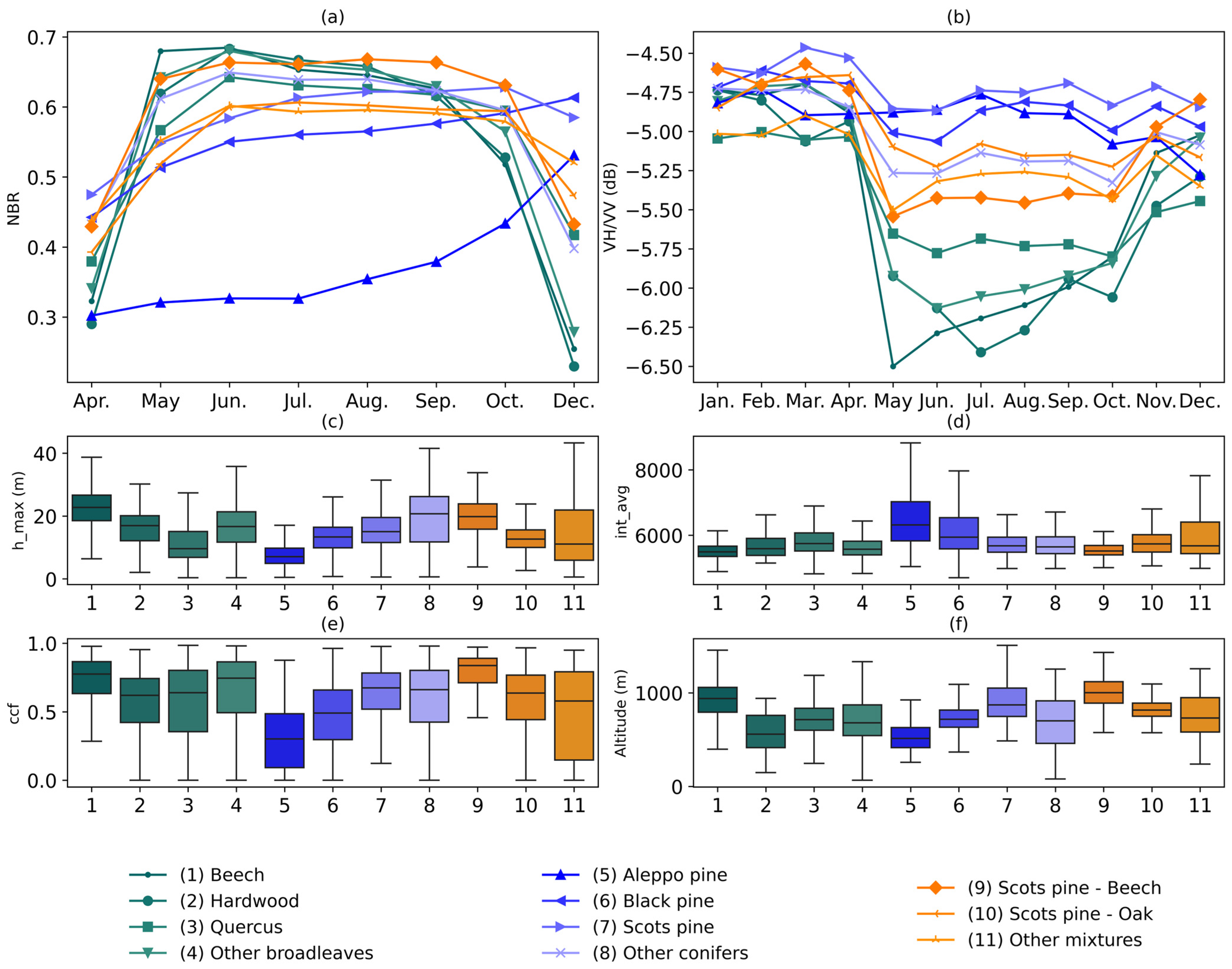
4.1. Descriptive Analysis

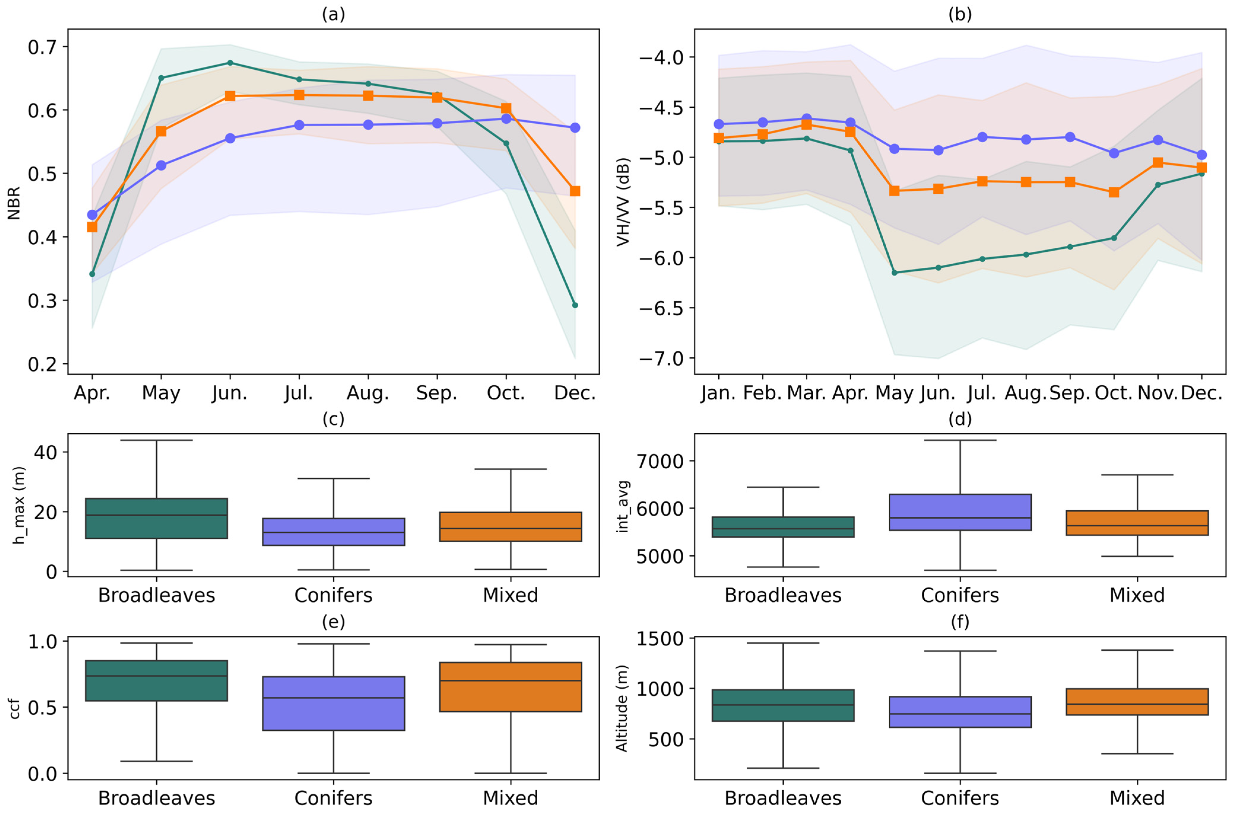
The median time series of broadleaves, conifers, and mixed forests for the S-2 NBR and the S-1 VH/VV ratio, as well as the boxplots of some selected LiDAR metrics (maximum height, average intensity, and canopy cover fraction), and the altitude are plotted in Figure 3. Results for levels 2 and 3 are given in Appendix A (Figure A1 and Figure A2).

The values of NBR (Figure 3a) for broadleaves exhibited an increase in spring, followed by a decline from summer onwards, reaching the lowest values in December. In contrast, conifers showed a rather flat trend, with a slight increase in NBR during spring, but an almost flat trend from summer to autumn. Mixed forests had an intermediate NBR trend, positioned between conifers and broadleaves. The month of December exhibited the greatest difference between the three classes. The variability of the NBR was found to be the highest for conifers, although differences were not significant.

The time series of S-1 features spanned from January to December (e.g., VH/VV in Figure 3b), thus enabling a more detailed multitemporal analysis than S-2. During the winter months of January to March, broadleaves, conifers, and mixed forests exhibited very similar VH/VV values, maintaining an almost constant value until the onset of spring. Beginning in April, VH/VV showed a sharp decline in broadleaves, reaching its minimum in May, and subsequently taking an upward trend from June to October (summer). Finally, broadleaves showed an increase in VH/VV in November, coinciding with the leaf fall. Conversely, conifers exhibited a relatively constant VH/VV trend, with minor fluctuations observed in May and October. Mixed forests showed again an intermediate behavior indicative of the mixture of coniferous and broadleaves. The largest differences between forest types in VH/VV occurred during the late spring and summer months.

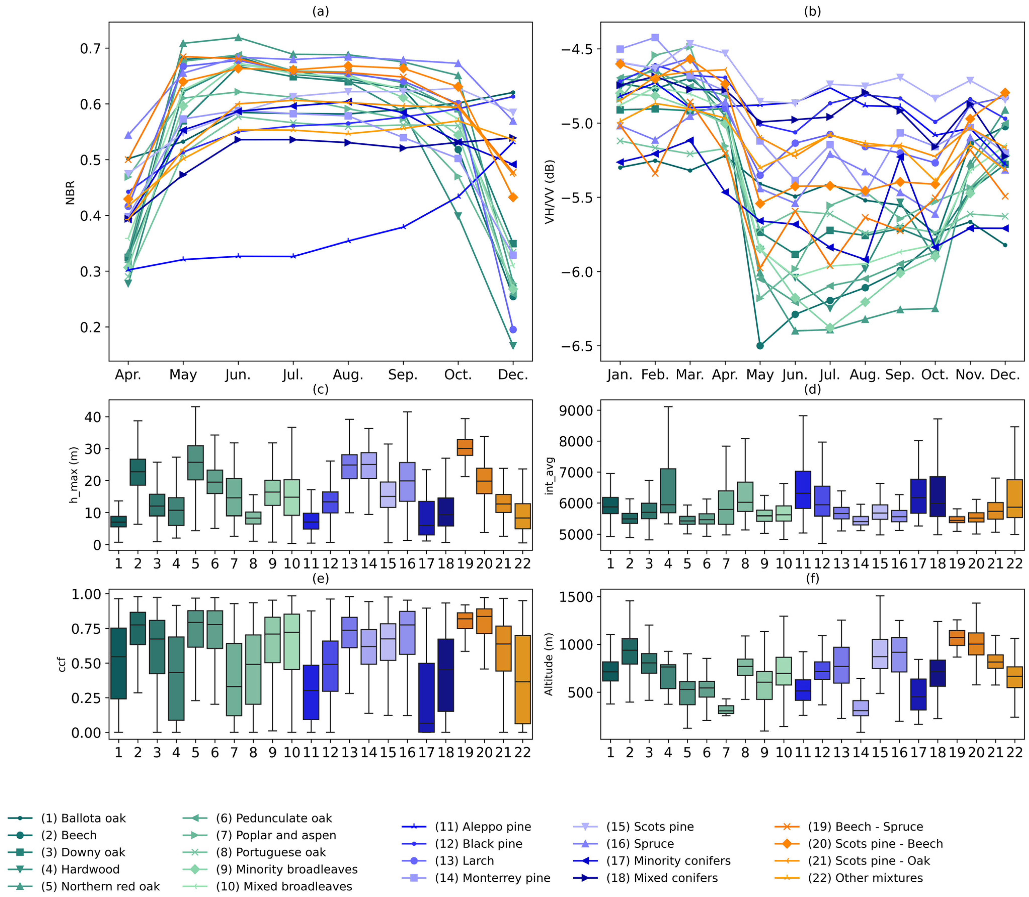
The distribution of the LiDAR metrics (Figure 3c–e) and the altitude (Figure 3f) demonstrated a substantial overlap between the three classes at level 1. The maximum height (h_max, Figure 3c) and canopy cover fraction (ccf, Figure 3d) were found to be slightly higher for broadleaves, while the average intensity was slightly higher for conifers. The distribution of forest types in terms of altitude was found to be quite similar. However, more detailed classification levels (levels 2 and 3) showed specific behaviors for certain species in the LiDAR metrics and topographic features (Figure A1 and Figure A2). Monospecific classes (e.g., Beech and Black pine) had the smallest interquartile range (IQR) compared to more heterogeneous classes (e.g., Quercus and other conifers). Furthermore, substantial differences were also observed among the broadleaved classes and among the conifer classes, due to the specificities of each species. Additionally, mixed forest classes exhibited different values depending on the monospecific classes intervening in the mixture (Figure A1 and Figure A2) (e.g., similar altitude data distributions for Beech and Scots pine-Beech classes).

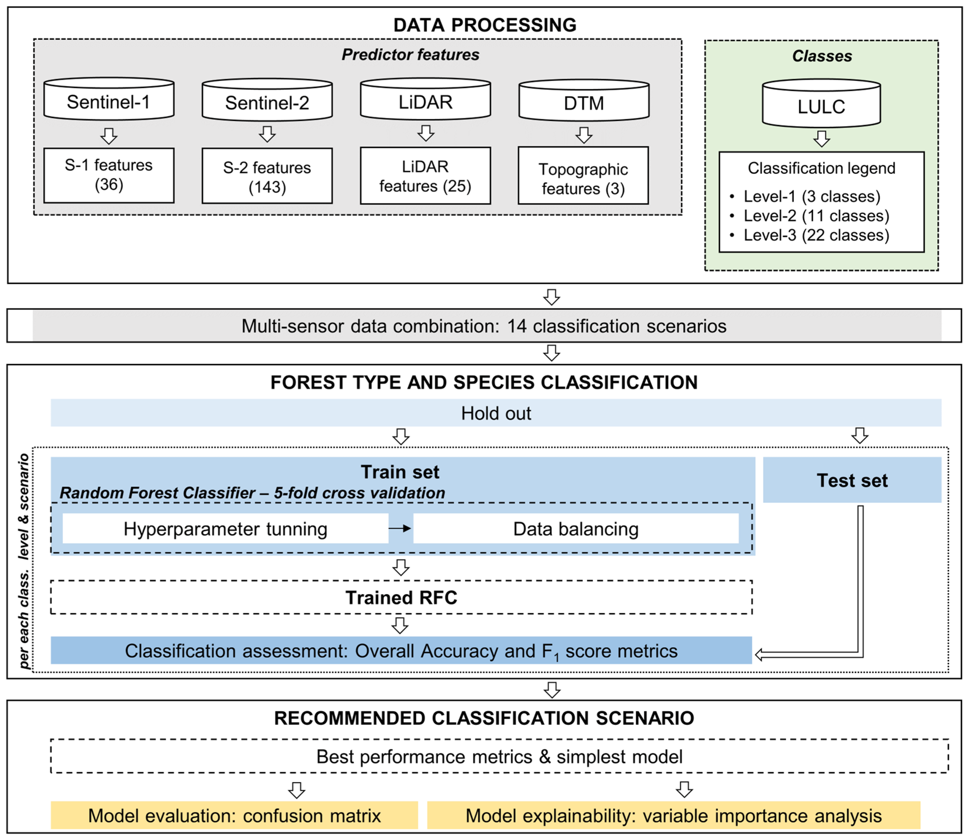
4.2. Classification Results

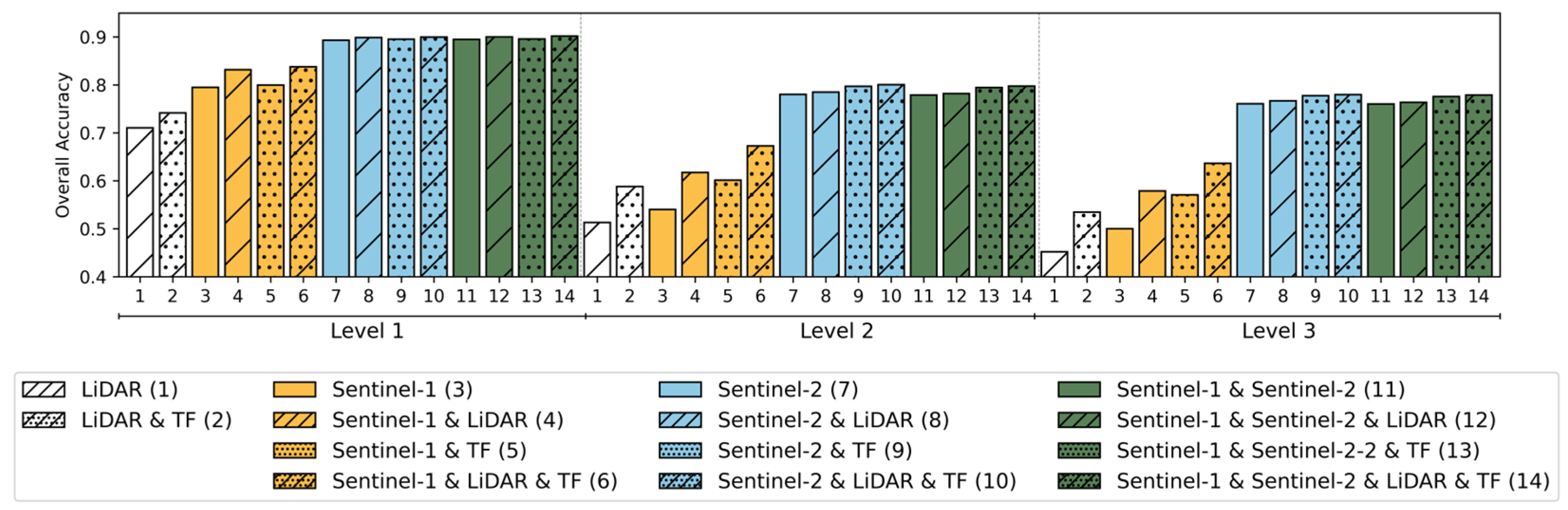
Figure 4 shows the OA values obtained with the test dataset for the different classification models. In all cases, the OA obtained for each particular model decreased as the classification level became more specific, with this decrease being more pronounced when moving from level 1 to level 2 than from level 2 to level 3. In addition, the three levels showed analogous patterns with regard to the classification scenarios. On the one hand, the scenarios including S-2 (scenarios 7–14) yielded the highest OA, followed by those including S-1 (scenarios 3–6) and LiDAR (1–2). On the other hand, the incorporation of topographic variables enhanced the OA in the majority of cases. However, the OA gain brought by these topographic variables was less pronounced at level 1 than at levels 2 and 3. The incorporation of LiDAR metrics to S-1 and/or S-2 scenarios led to an enhancement in OA in all cases, with greater enhancements for S-1 than for S-2.

For level 1, scenarios 8, 10, 12, and 14 displayed the highest OA values (~0.90), while, for levels 2 and 3, scenarios 9, 10, and 14 performed the best (~0.80 for level 2 and ~0.79 for level 3). It is worth noting that the classification scenario based solely on S-2 data (7) already achieved high OA values, with only slight improvements when other datasets were incorporated (scenarios 8–14).

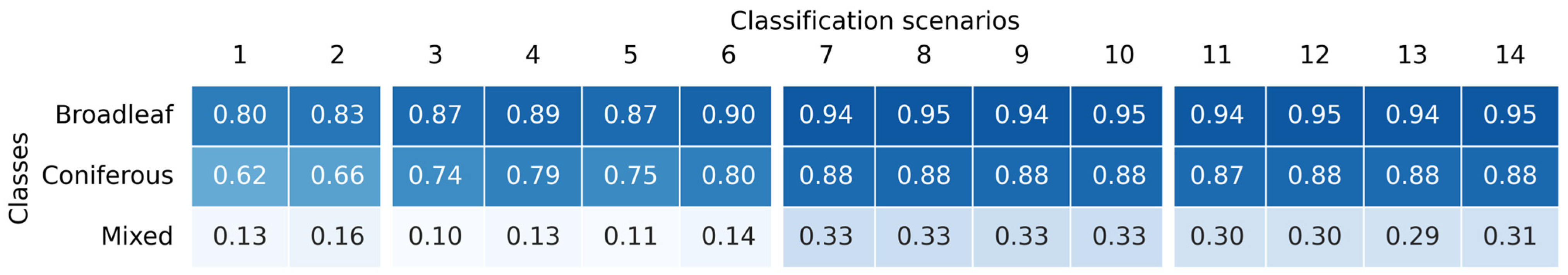
For a better understanding of the classification results, the F₁ score values of each class are presented in Figure 5, Figure 6 and Figure 7. Generally, it was observed that the benefits of combining input data were more significant for more complex classification levels (2 and 3). For level 1 (Figure 5), broadleaves achieved the lowest error in all scenarios, with F₁ scores ranging from 0.80 to 0.95, followed by conifers (F₁ of 0.62–0.88) and mixed forests (F₁ of 0.13–0.33). The difference in F₁ values between broadleaves and conifers was higher in the first six scenarios. Notably, scenarios based on S-2 (7 to 14) yielded the highest accuracies, with remarkable F₁ values for both broadleaves and conifers. Interestingly, the combination of S-1 and S-2 (scenarios 11 to 14) did not yield any enhancements in comparison to those based on S-2 alone (scenarios 7 to 10). In fact, the results obtained for broadleaves and conifer forests remained unchanged after adding S-1, whereas the mixed class obtained an even poorer F₁ score. Indeed, the mixed class achieved very low F₁ scores in classifications based on S-1 data (scenarios 3 to 6). However, quite good results were obtained with S-1 for broadleaves and conifer forests, especially when incorporating the LiDAR metrics (scenario 4) and, to a lesser extent, the topographic variables (scenario 6), reaching F₁ scores of 0.90 and 0.80 for broadleaves and conifers, respectively.

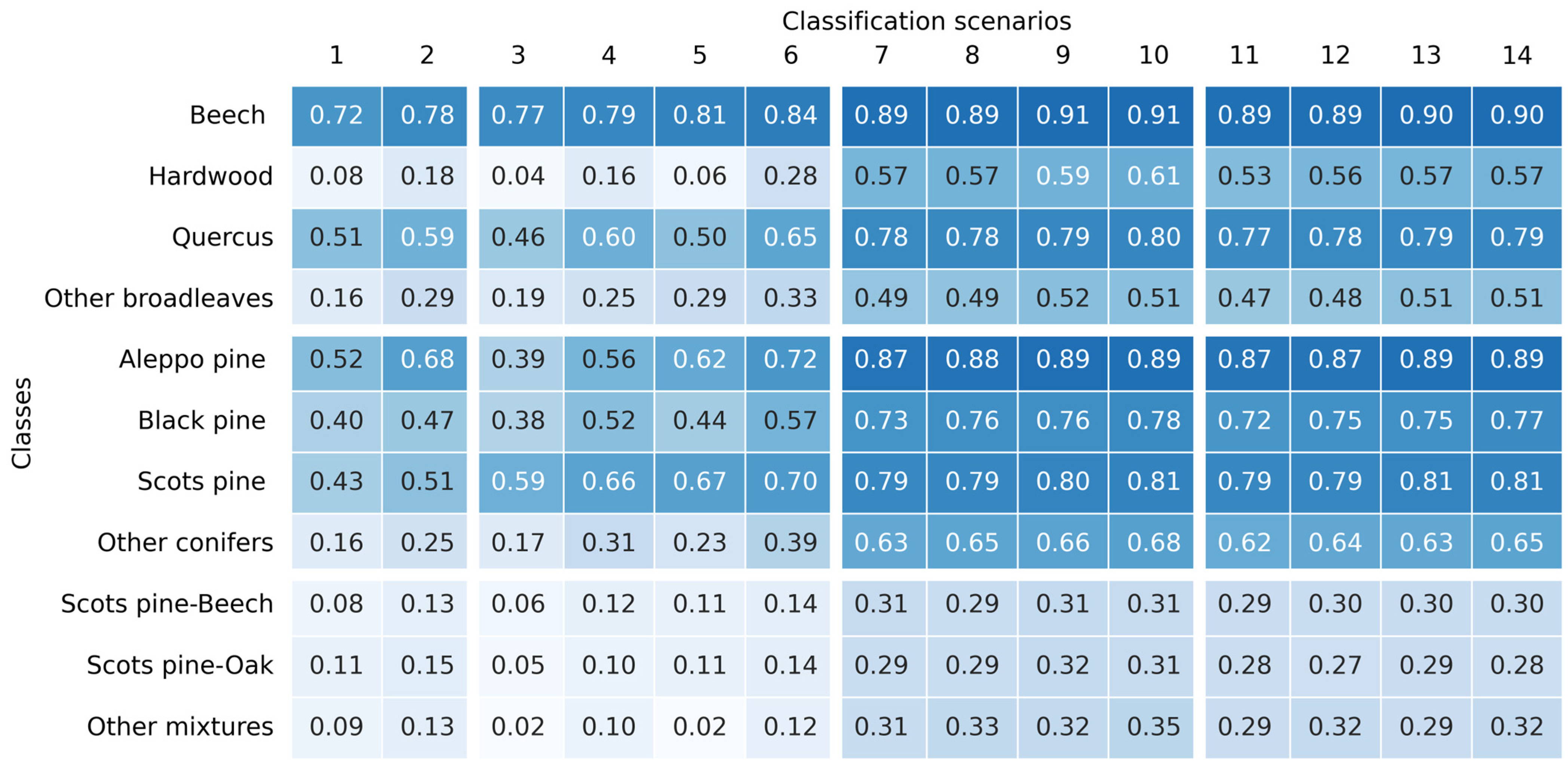
In level 2 (Figure 6), the species achieving the highest F₁ scores were Beech, Aleppo pine, Scots pine, Quercus, and Black pine across most of the classification scenarios. Indeed, the models demonstrated a superior performance when classifying homogeneous classes, as opposed to heterogeneous classes (e.g., hardwood, other conifers, and other mixtures). In a manner analogous to the results observed for level 1, the incorporation of S-2 bands in the classifications led to an enhancement in the accuracy of these heterogeneous and mixed classes. Furthermore, scenarios based on S-2 (from 7 to 10) outperformed those combining S-1 and S-2 (from 11 to 14) across nearly all classes. Beech was the only species achieving an F₁ score greater than 0.70 using only LiDAR and topographic variables as model inputs (scenarios 1 and 2). In the other scenarios, the incorporation of LiDAR and/or topographic variables had a positive effect on the classification results. In some classes, LiDAR exhibited a greater impact than topographic variables (e.g., Hardwood and Quercus), while in other classes the reverse was observed (e.g., Aleppo pine). However, for the majority of species (e.g., Beech and Scots pine), there was a minimal difference in the results, especially when F₁ scores were already high (>0.70). Finally, it is worth noting that, while scenarios based on S-2 and S-1 and S-2 achieved the highest accuracies for most classes, scenario 6 (S-1) also yielded high accuracies for specific species, such as Beech (0.84), Aleppo pine (0.72), and Scots pine (0.70).

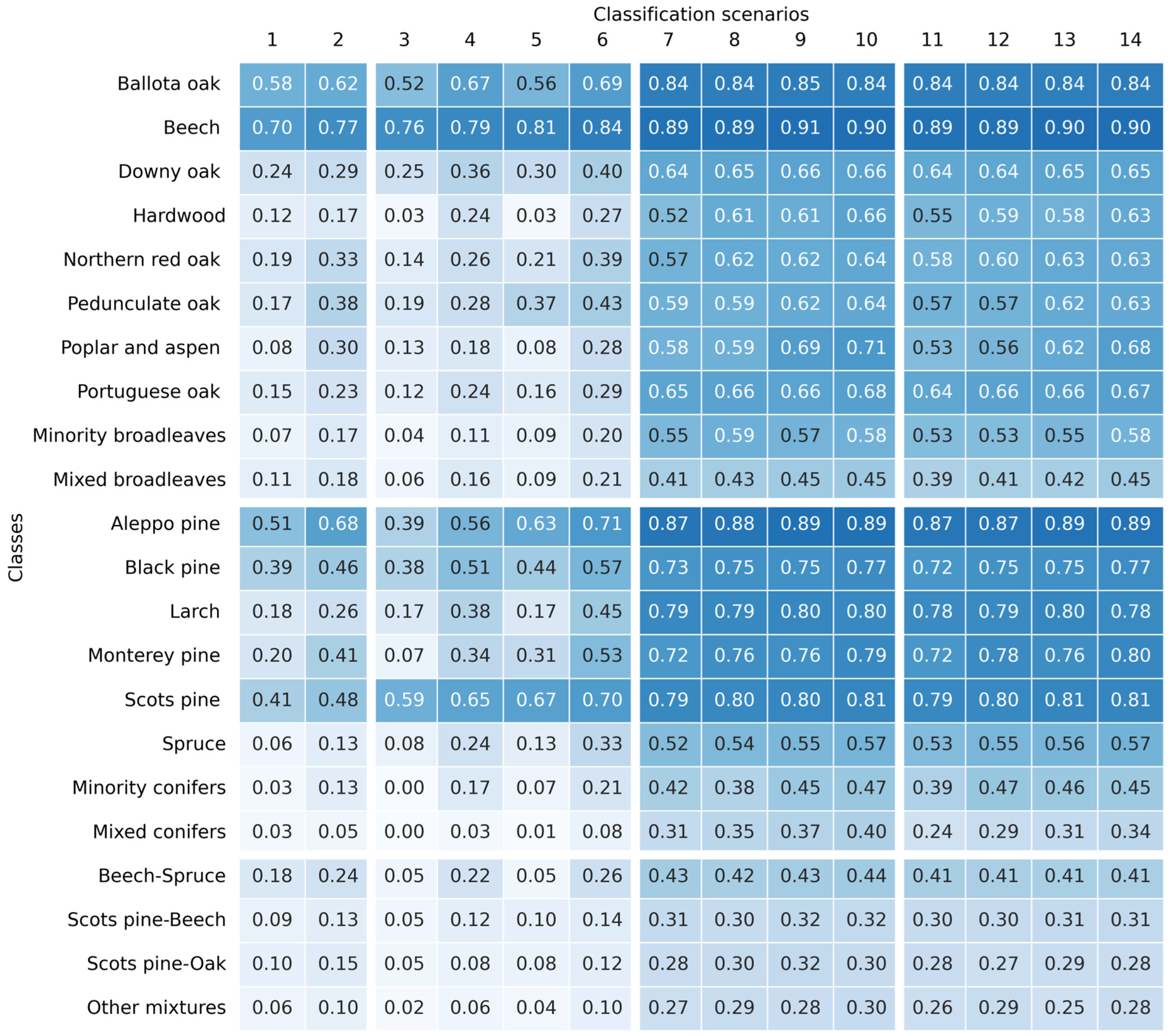
Finally, for classification level 3 (Figure 7), Beech, Aleppo pine, Scots pine, and Black pine classes maintained mostly the same F₁ scores achieved for level 2, being again the best classified species. Additionally, Ballota oak, Larch, and Monterey pine demonstrated noteworthy performances, achieving high F₁ scores. Conversely, Northern red, Pedunculate and Portuguese oak, and Spruce were identified as the most challenging monospecific classes. Nevertheless, the performance of mixed and heterogeneous classes was again the poorest.

At level 3, in an analogous manner to level 2, most classes obtained higher accuracies when using S-2 as input (scenarios 7–14), in comparison to S-1 or LiDAR (scenarios 1–6), with most notable examples being Hardwood, Larch and Monterey pine, followed by Downy and Portuguese oaks, Black pine and Spruce. The contribution of S-2 bands was also remarkable for mixed and heterogeneous classes, which obtained modest performances, but in any case, much higher than with S-1 or LiDAR. As for level 2, the addition of LiDAR and topographic variables to the classification models based on S-1 and/or S-2 generally leads to enhanced F₁ scores. In general, similar improvements were obtained when adding either LiDAR or topographic data, but in some cases, topographic features appeared to be more determinant (e.g., Poplar and aspen), and in some others, LiDAR (e.g., Hardwood, Black and Monterey pines, and Beech-spruce mixtures).

For most level 3 classes, scenarios incorporating S-2 data yielded the highest F₁ scores. However, it should be noted that certain classes exhibited already remarkable F₁ values even in the absence of this data. In scenario 2 (LiDAR and topographic data), Beech and Aleppo pine exhibited adequate results, achieving F₁ scores of 0.77 and 0.68, respectively. These performances were further enhanced when S-1 data was integrated in scenario 6, with Beech attaining an F1 score of 0.84 and Aleppo pine 0.71. Scots pine also obtained promising results in this scenario, with an F₁ score of 0.70.

The findings indicate that scenarios 9, 10, and 14 yielded the most favorable results for the three classification levels. Scenario 9 (S-2) presented high performance metrics with a lower number of input variables than scenario 10 (S-2 and topographic features). However, certain classes, such as Hardwood or Monterey pine, exhibited a substantial enhancement in their classification metrics in scenarios 10 and 14 (all input datasets). Regarding model complexity, classification scenario 10 was simpler than scenario 14. Consequently, the classification model selected as the one achieving the best compromise in terms of accuracy and model complexity was scenario 10. This model was thus recommended, and it was further evaluated in the next sections.

4.3. Recommended Classification Scenario

This section comments on the confusion matrices obtained with the recommended classification model (scenario 10), across all three levels, to evaluate the confusion between classes. At level 1 (

Table 5. Confusion matrix for scenario 10 at level 1. Values in the matrix represent the number of samples.

	Level 1	Predicted Class
		Broadleaves	Conifers	Mixed	Total
Ground truth	Broadleaves	32,962	1147	854	34,963
	Conifers	1098	14,271	663	16,032
	Mixed	682	906	748	2336
	Total	34,742	16,324	2265	53,331
UA		0.95	0.87	0.33
PA		0.94	0.89	0.32
OA					0.90

PA: Producer’s Accuracy, UA: User’s Accuracy, OA: Overall Accuracy.

), the mixed class had the highest level of confusion, with only 32% (PA) of the test samples being correctly classified. Misclassified samples were confused with both conifers and broadleaves, although a higher degree of confusion was observed with conifers. In contrast, 94% of broadleaves and 89% of conifer test samples were correctly classified. Some confusion between broadleaves and conifers occurred. However, it had a minimal impact on the results. Approximately 3.3% of broadleaves were misclassified as conifers, while 6.8% of conifers were incorrectly classified as broadleaves.

Regarding the confusion matrix obtained at level 2 (

Table 6. Confusion matrix for scenario 10 at level 2. Values in the matrix represent the number of samples.

Level 2		Predicted Class
Ground Truth		Broadleaves				Conifers				Mixed
		1	2	3	4	5	6	7	8	9	10	11	Total
Broadleaves	1	17,414	4	441	849	2	5	162	58	395	20	93	19,443
	2	17	86	10	54	0	6	0	2	0	0	0	175
	3	485	10	9501	1213	179	116	271	54	56	248	36	12,169
	4	673	7	467	1897	10	4	31	36	37	12	2	3176
Conifers	5	0	0	108	6	3460	120	22	6	0	1	19	3742
	6	4	0	217	14	132	2502	253	30	1	15	29	3197
	7	114	0	451	41	62	343	6372	33	222	266	16	7920
	8	66	0	49	77	79	66	81	723	7	5	20	1173
Mixed	9	147	0	46	22	0	1	168	4	262	19	1	670
	10	8	0	250	17	3	21	392	2	40	297	1	1031
	11	62	0	117	10	90	73	73	18	4	6	182	635
	Total	18,990	107	11,657	4200	4017	3257	7825	966	1024	889	399	53,331
UA		0.92	0.80	0.82	0.45	0.86	0.77	0.81	0.75	0.26	0.33	0.46
PA		0.90	0.49	0.78	0.60	0.92	0.78	0.80	0.62	0.39	0.29	0.29
OA													0.80

1: Beech, 2: Hardwood, 3: Quercus, 4: Other broadleaves, 5: Aleppo pine, 6: Black pine, 7: Scots pine, 8: Other conifers, 9: Scots pine–Beech, 10: Scots pine–Oak, and 11: Other mixtures. PA: Producer’s Accuracy, UA: User’s Accuracy, OA: Overall Accuracy.

), the most important species had little confusion. For instance, 90% (PA) of the Beech test samples (class 1 in Table 6) were correctly classified, 4% were misclassified as other broadleaves, 2% as Quercus, and 2% as Scots pine–Beech mixed forests. Conversely, within the 18,990 samples classified as Beech, 3% were actually other broadleaves, and 4% were Quercus. Similarly, 92% of the Aleppo pine test samples were correct, with only a few errors with Quercus and Black pine. Concerning Scots pine, 80% of its samples were correct, and confusion occurred with Quercus (6%), Black pine (4%), and mixed classes like Scots pine-Beech and Scots pine-Oak (3%).

Looking at the mixed classes (Table 6), it was noteworthy that only 26% (UA) of the samples assigned to the Scots pine-Beech class really belonged to it. However, the confusion occurred with the monospecific classes intervening in the mix (Beech and Scots pine). Similar results were observed for the Scots pine-Oak mixed class.

At level 3 (

Table 7. Confusion matrix for scenario 10 at level 3. Values in the matrix represent the number of samples.

L3	Predicted Class
Ground	Broadleaves										Conifer								Mixture
Truth	1	2	3	4	5	6	7	8	9	10	11	12	13	14	15	16	17	18	19	20	21	22	Total
1	3915	8	116	0	0	0	1	30	0	30	113	38	0	0	104	2	0	3	0	3	24	23	4410
2	19	17,345	441	2	31	252	0	4	7	579	5	6	11	0	144	43	2	2	129	407	12	2	19,443
3	101	205	2822	1	4	67	0	83	9	264	8	20	0	0	121	1	0	2	0	36	152	4	3900
4	0	8	5	33	0	1	0	0	0	7	0	5	0	0	1	1	0	1	0	0	0	0	62
5	0	31	4	0	298	61	0	0	0	42	0	1	2	4	0	4	0	0	0	0	0	0	447
6	0	169	51	1	68	1161	0	0	16	152	2	5	5	5	1	2	2	0	0	0	0	2	1642
7	1	0	0	0	0	0	31	0	0	13	0	0	0	0	0	0	0	0	0	0	0	0	45
8	47	0	106	0	0	3	0	589	0	8	10	39	0	0	5	0	0	0	0	0	11	10	828
9	1	42	28	0	4	37	0	1	208	92	2	2	0	2	0	1	0	0	0	0	0	0	420
10	343	696	450	0	68	387	10	85	49	1497	32	9	10	8	38	4	1	6	0	46	17	10	3766
11	71	0	24	0	0	0	0	11	1	9	3454	113	0	1	26	0	0	7	0	0	3	22	3742
12	94	6	55	1	0	6	0	49	0	11	125	2487	3	3	277	5	5	7	0	2	13	48	3197
13	0	45	10	0	4	12	0	0	0	11	0	0	300	0	8	8	0	1	0	3	0	0	402
14	0	4	0	0	6	8	0	0	1	9	0	1	2	136	2	10	0	0	0	1	0	0	180
15	194	121	254	0	0	1	0	16	0	43	71	354	7	1	6319	13	0	4	4	222	280	16	7920
16	2	16	9	0	0	6	0	0	2	13	0	2	4	1	29	155	4	1	14	2	2	0	262
17	0	0	1	0	1	1	0	1	0	3	7	7	0	1	2	7	20	0	0	0	0	1	52
18	9	5	7	0	0	0	0	1	0	8	64	43	4	2	43	5	0	78	0	4	2	2	277
19	0	45	0	0	0	0	0	0	0	1	0	0	0	0	6	17	0	0	86	0	0	0	155
20	5	152	45	0	0	2	0	0	0	11	0	5	1	0	158	3	0	0	2	268	18	0	670
21	35	8	217	0	0	1	0	26	0	15	4	23	1	0	389	1	0	0	0	33	275	3	1031
22	57	10	29	0	0	4	0	13	0	14	86	76	2	0	65	1	0	1	0	4	7	111	480
Total	4894	18,916	4674	38	484	2010	42	909	293	2832	3983	3236	352	164	7738	283	34	113	235	1031	816	254	53,331
UA	0.89	0.89	0.72	0.53	0.67	0.71	0.69	0.71	0.50	0.40	0.92	0.78	0.75	0.76	0.80	0.59	0.38	0.28	0.55	0.40	0.27	0.23
PA	0.80	0.92	0.60	0.87	0.62	0.58	0.74	0.65	0.71	0.53	0.87	0.77	0.85	0.83	0.82	0.55	0.59	0.69	0.37	0.26	0.34	0.44
OA																							0.78

1: Ballota oak, 2: Beech, 3: Downy oak, 4: Hardwood, 5: Northern red oak, 6: Pedunculate oak, 7: Poplar and aspen, 8: Portuguese oak, 9: Minority broadleaves, 10: Mixed broadleaves, 11: Aleppo pine, 12: Black pine, 13: Larch, 14: Monterey pine, 15: Scots pine, 16: Spruce, 17: Minority conifers, 18: Mixed conifers, 19: Beech-Spruce, 20: Scots pine-Beech, 21: Scots pine-Oak, 22: Other mixtures. PA: Producer’s Accuracy, UA: User’s Accuracy, OA: Overall Accuracy.

), similar results were observed, with the main monospecific classes being correctly classified, and most of the confusion occurring in heterogeneous and mixed classes. For broadleaves, Beech and Ballota Oak test samples were correctly classified in 89% of the cases, with only a minor confusion with Mixed broadleaves and Downy oak, and in the case of Ballota Oak also with some conifers (Aleppo and Scots pines). The most challenging broadleaves categories were the heterogeneous ones, specifically the hardwood class, with only 53% of its samples being correctly identified, and a large confusion with Beech, Downy oak, Mixed broadleaves, and Black pine. Interestingly, 87% (UA) of the samples assigned to Hardwood were correct. While half of the minority broadleaves samples were correctly classified, with the rest being mostly confused with other broadleaves (10%), beech (2%), and downy oak (3%).

Regarding conifers, Aleppo pine maintained 92% of correctly classified test samples, consistent with the results at level 2, and with only a few errors with Black pine and Ballota oak. Scots pine also obtained successful results with 80% of samples correctly classified, and the main confusions were with the mixed classes where this species participated. It was also noteworthy that nearly 11% of samples misclassified as Black pine belonged to the Scots pine category. Less frequent conifers like Larch or Monterey pine were, in general, correctly classified. In contrast, Spruce showed both poor PA and UA results, with only 59% of its samples correctly assigned, and notable confusion with Scots pine, Scots pine-Beech, and Beech classes. Minority and mixed conifers showed the worst results, with a substantial proportion of their samples wrongly assigned to Aleppo pine and, to a lesser extent, to other conifer species.

Finally, regarding mixed classes, in accordance with the already commented F₁ scores (Figure 7), results were less successful, but the confusion matrix (Table 7) showed that confusion mostly occurred with the monospecific classes intervening in the mix. For instance, the Beech–Spruce class was mostly confused with the Beech and Spruce classes, and the same occurred with Scots pine–Beech and Scots pine–Oak classes.

4.4. Classification Model Explainability

The 15 predictor variables with the highest Gini index (MDG) are ranked in Figure 8. For level 1, the S-2 images acquired in June and July emerged as pivotal predictor variables, particularly the NIR and red-edge bands (i.e., B06, B07, B08, and B8A). Interestingly, no LiDAR features achieved a high importance rank in level 1. Conversely, in levels 2 and 3, the altitude emerged as the most significant feature, exhibiting a substantial difference from the rest. Furthermore, LiDAR height metrics (max, p95, and p90) were also identified as important features at levels 2 and 3. It is noteworthy that at these more detailed levels, the S-2 December composite, and, in particular, its vegetation indices (NDII, NBR, and NDVI), demonstrated a high importance ranking, higher than for level 1.

5. Discussion

The classification scenarios based exclusively on LiDAR data (scenarios 1 and 2) obtained low accuracies, revealing a limited capacity of LiDAR features in discriminating among forest types and species. Previous studies [23,53] reported similar accuracies (0.66 and 0.62, respectively) when classifying six forest types with LiDAR data, supporting the notion that LiDAR metrics should be best used as ancillary data in forest classification procedures that rely on multispectral observations [54,55]. In contrast, Trouvé et al. [56] achieved an OA of 0.81 when classifying Rainforest, Mixed Forest, Fern-dominated stands and Eucalyptus-dominated stands in Victoria (Australia), outperforming a classification based on S-2 multispectral data. This remarkable result was probably related to the less complex forest system assessed, in addition to the high density of the LiDAR dataset used in their study (28.1 pts/m²), which enabled the extraction of more detailed structural metrics of individual trees, which were key in distinguishing forest classes with relevant overstorey vegetation.

The results obtained from S-1 SAR data (scenario 3) were modest in comparison to those based on S-2. Direct comparisons with other SAR based studies are challenging due to differences in SAR data, and other experimental details. However, the results obtained in the present study align with the findings of Rüetschi et al. [57] or Dostalova et al. [58] who reported an OA of 0.82–0.86 for broadleaves-conifers classifications using S-1 data. It is worth highlighting that these two investigations did not consider a mixed-forest class, as in our study. Furthermore, Rüetschi et al. [57] considered a rather simple species composition (only three broadleaved species: Fagus sylvatica, Quercus robur and Quercus petraea, and one conifer: Norway spruce). Conversely, our broadleaves and conifers classes include a considerably higher number of species (ten broadleaves and eight conifers) (Table 2). Lechner et al. [32] employed a more intricate legend, including 12 monospecific classes (7 broadleaves and 5 conifers), using S-1 data. However, their performance was found to be inferior, with an OA of 0.56.

The classification scenario based on S-2 data (scenario 7) yielded significantly higher accuracies compared to those based solely on LiDAR or S-1. These results were close to the OA of 0.88 obtained by Persson et al. [59], who used multi-temporal S-2 data to classify five species in Sweden. Similarly, Grabska et al. [12] used S-2 time series to classify nine tree species in the Carpathian Mountains, obtaining an OA of 0.92. In contrast, Liu et al. [60] classified eight forest types in Wuhan, and reported an OA of 0.53 when S-2 was used as input. It should be highlighted that few studies considered mixed or heterogeneous classes in their classification legends. This is an important detail that makes our study particularly challenging, since most heterogeneous classes yielded low F₁ scores, thereby reducing the OA of the model. However, it is noteworthy that the confusion of the mixed classes mainly occurred with the monospecific classes intervening in the mix (Figure 5, Figure 6 and Figure 7). Taking into account that our classification approach is implemented at the pixel scale, these errors are expected to be rather unimportant from the user’s standpoint.

Classifications based on S-2 obtained even higher OA values when LiDAR and/or topographic variables were incorporated (scenario 8–10), as also observed by Iglseder et al. [61]. The combination of LiDAR and S-1 data (scenario 4) also resulted in substantial improvements. This underscores the complementary of S-1 and LiDAR data, further emphasizing their unique contributions. SAR backscatter depends on the dielectric and geometric properties of forest stands [20], but the latter seems to be complementary to the geometric attributes sensitive to LiDAR.

The benefit of the combination of input variables was also observed in other similar studies [27,62,63]. Plakman et al. [14] reported the highest classification results when S-2 and LiDAR data were combined for mapping species at the individual tree scale in the Netherlands. They also highlighted how the LiDAR structural parameters could improve the classification of species with similar spectral properties but different structural characteristics. This was the case of the Black pine and Scots pine in our study, whose spectral behavior is similar, but their height and structure are different.

In our study, the integration of S-1 and S-2 data (scenarios 11 to 14) did not yield significant improvements in the OA when compared to classifications based only on S-2 data (scenarios 7–10). S-1 and S-2 integration did not bring any improvements in the F₁ scores of the main species. In fact, in some cases, it actually led to a decline in classification performance, especially in heterogeneous classes like Mixed conifers or Other mixtures. Similar results were observed in the literature [31,64,65]. The lack of improvement from the inclusion of S-1 data may be attributed to the redundancy of the information it provides in this specific context. S-2 data already captures relevant key spectral traits of tree species. Therefore, S-1 did not appear to contribute additional, complementary information, and its inclusion increased model complexity.

The S-2 summer acquisitions (June–August), particularly the NIR and red-edge bands, were identified as the most important input features for the three classification levels. Praticò et al. [45] reported the best OA results when classifying Mediterranean forest habitats with summer data, arguing that the vegetative species are in their maximum growth period. Consistent findings were obtained by Persson et al. [59], where late spring imagery showed the best classification results, indicating that the phenological variations in this period were most pronounced. Lisein et al. [66] also reported that late spring and early summer images were important for discriminating deciduous tree species. These results are consistent with the time series depicted in Figure 3a (Figure A1a and Figure A2a). VIs in broadleaves exhibited the typical seasonal pattern of spring-increase, summer-peak, and autumn-decline. In contrast, most coniferous species showed a lower seasonal variability in their VI curves, with a rather flat trend, except for a minor increase in spring. Aleppo pine displayed a different trend, probably due to the typical summer drought in the southern Navarre region, where this species is predominant.

At levels 2 and 3, the topographic altitude also appeared to be important for forest species classification. This result underscores the idea that in rugged areas (such as Navarre), species distribution is conditioned by the topography, and thus adding this ancillary variable is helpful in forest species mapping. Similar results were reported by Hościło and Lewandowska [67]. Nevertheless, it is important to be careful when incorporating the altitude or other topographic features into forest classification models, and to ensure that the training data encompasses the entire altitudinal range of all tree species. This is particularly pertinent when employing Random Forest as a classifier, given that this algorithm does not extrapolate.

6. Conclusions

The results of this investigation are relevant given the limited number of studies assessing the combination of SAR, optical, and LiDAR data. Furthermore, the complexity of the three-level classification legend is considered, and its high species diversity is also particularly challenging. The results demonstrate the potential of combining data from different Earth observation technologies to enhance the mapping of forest types and species. A comparison of single-sensor configurations showed optimal classification results for Sentinel-2, outperforming Sentinel-1 and LiDAR, particularly at classification levels 2 and 3 (with 11 and 22 forest classes, respectively). The NIR and red-edge bands of summer acquisitions were identified as the most significant features for achieving successful classification. Sentinel-1 obtained a lower accuracy, yet it was able to classify forest types (broadleaves, conifers, and mixed forests) with an accuracy of 0.8. LiDAR data alone did not yield adequate classification results, but its incorporation into Sentinel-2 or Sentinel-1-based classifications led to improvements in accuracy, particularly for Sentinel-1. This finding demonstrates that the structural information provided by LiDAR sensors is complementary to the spectral information. In turn, the combination of Sentinel-1 and Sentinel-2 data did not yield further enhancements, and in some cases, it led to a decline in the F₁ score values for certain species. Furthermore, the incorporation of topographic features to Sentinel-1, Sentinel-2, and LiDAR classifications yielded enhanced accuracies, particularly for those species whose distribution is typical of specific altitudinal ranges. Yet, the incorporation of topographic features might not offer significant benefits in other areas where topography is not relevant. For classification levels with higher complexity (levels 2 and 3), monospecific classes achieved higher accuracies than mixed classes. The latter, in fact, were the ones contributing the most to classification errors, but confusion mainly occurred with the monospecific classes intervening in the mix. To confirm the findings of this study, analogous studies should be performed in regions with different forest types and species. To enhance the robustness and interpretability of the classification methodology, future improvements could focus on incorporating a deeper analysis of predictor variable importance and implementing model explainability techniques such as Shapley Additive exPlanations (SHAP).

References

1. Acharya, R.P.; Maraseni, T.; Cockfield, G. Global Trend of Forest Ecosystem Services Valuation—An Analysis of Publications. Ecosyst. Serv. 2019, 39, 100979. [Google Scholar] [CrossRef]
2. FAO Natural Forest Management. Available online: https://www.fao.org/4/w7715e/w7715e04.htm (accessed on 25 October 2023).
3. Thompson, I.; Mackey, B.; McNulty, S.; Mosseler, A. Forest Resilience, Biodiversity, and Climate Change. A Synthesis of the Biodiversity/Resilience/Stability Relationship in Forest Ecosystems; Technical Series; Secretariat of the Convention on Biological Diversity: Montreal, QC, Canada, 2009; ISBN 978-92-9225-137-6. [Google Scholar]
4. Holzwarth, S.; Thonfeld, F.; Kacic, P.; Abdullahi, S.; Asam, S.; Coleman, K.; Eisfelder, C.; Gessner, U.; Huth, J.; Kraus, T.; et al. Earth-Observation-Based Monitoring of Forests in Germany—Recent Progress and Research Frontiers: A Review. Remote Sens. 2023, 15, 4234. [Google Scholar] [CrossRef]
5. FAO Global Forest Resources Assessment 2020: Main Report; FAO: Rome, Italy, 2020; ISBN 978-92-5-132974-0.
6. Shirazinejad, G.; Javad Valadan Zoej, M.; Latifi, H. Applying Multidate Sentinel-2 Data for Forest-Type Classification in Complex Broadleaf Forest Stands. For. Int. J. For. Res. 2022, 95, 363–379. [Google Scholar] [CrossRef]
7. Lines, E.R.; Fischer, F.J.; Owen, H.J.F.; Jucker, T. The Shape of Trees: Reimagining Forest Ecology in Three Dimensions with Remote Sensing. J. Ecol. 2022, 110, 1730–1745. [Google Scholar] [CrossRef]
8. Abad-Segura, E.; González-Zamar, M.-D.; Vázquez-Cano, E.; López-Meneses, E. Remote Sensing Applied in Forest Management to Optimize Ecosystem Services: Advances in Research. Forests 2020, 11, 969. [Google Scholar] [CrossRef]
9. Zhang, W.; Liu, X.; Xu, B.; Liu, J.; Li, H.; Zhao, X.; Luo, X.; Wang, R.; Xing, L.; Wang, C.; et al. Remote Sensing Classification and Mapping of Forest Dominant Tree Species in the Three Gorges Reservoir Area of China Based on Sample Migration and Machine Learning. Remote Sens. 2024, 16, 2547. [Google Scholar] [CrossRef]
10. Gibson, R.; Danaher, T.; Hehir, W.; Collins, L. A Remote Sensing Approach to Mapping Fire Severity in South-Eastern Australia Using Sentinel 2 and Random Forest. Remote Sens. Environ. 2020, 240, 111702. [Google Scholar] [CrossRef]
11. Shen, W.; Li, M.; Huang, C.; Tao, X.; Li, S.; Wei, A. Mapping Annual Forest Change Due to Afforestation in Guangdong Province of China Using Active and Passive Remote Sensing Data. Remote Sens. 2019, 11, 490. [Google Scholar] [CrossRef]
12. Grabska, E.; Hostert, P.; Pflugmacher, D.; Ostapowicz, K. Forest Stand Species Mapping Using the Sentinel-2 Time Series. Remote Sens. 2019, 11, 1197. [Google Scholar] [CrossRef]
13. Hamrouni, Y.; Paillassa, E.; Chéret, V.; Monteil, C.; Sheeren, D. From Local to Global: A Transfer Learning-Based Approach for Mapping Poplar Plantations at National Scale Using Sentinel-2. ISPRS J. Photogramm. Remote Sens. 2021, 171, 76–100. [Google Scholar] [CrossRef]
14. Plakman, V.; Janssen, T.; Brouwer, N.; Veraverbeke, S. Mapping Species at an Individual-Tree Scale in a Temperate Forest, Using Sentinel-2 Images, Airborne Laser Scanning Data, and Random Forest Classification. Remote Sens. 2020, 12, 3710. [Google Scholar] [CrossRef]
15. Ferreira, M.P.; Wagner, F.H.; Aragão, L.E.O.C.; Shimabukuro, Y.E.; De Souza Filho, C.R. Tree Species Classification in Tropical Forests Using Visible to Shortwave Infrared WorldView-3 Images and Texture Analysis. ISPRS J. Photogramm. Remote Sens. 2019, 149, 119–131. [Google Scholar] [CrossRef]
16. Shimabukuro, Y.E.; Arai, E.; da Silva, G.M.; Dutra, A.C.; Mataveli, G.; Duarte, V.; Martini, P.R.; Cassol, H.L.G.; Ferreira, D.S.; Junqueira, L.R. Mapping and Monitoring Forest Plantations in Sao Paulo State, Southeast Brazil, Using Fraction Images Derived from Multiannual Landsat Sensor Images. Forests 2022, 13, 1716. [Google Scholar] [CrossRef]
17. Du, L.; Pang, Y.; Wang, Q.; Huang, C.; Bai, Y.; Chen, D.; Lu, W.; Kong, D. A LiDAR Biomass Index-Based Approach for Tree- and Plot-Level Biomass Mapping over Forest Farms Using 3D Point Clouds. Remote Sens. Environ. 2023, 290, 113543. [Google Scholar] [CrossRef]
18. Xu, D.; Wang, H.; Xu, W.; Luan, Z.; Xu, X. LiDAR Applications to Estimate Forest Biomass at Individual Tree Scale: Opportunities, Challenges and Future Perspectives. Forests 2021, 12, 550. [Google Scholar] [CrossRef]
19. Borlaf-Mena, I.; García-Duro, J.; Santoro, M.; Villard, L.; Badea, O.; Tanase, M.A. Seasonality and Directionality Effects on Radar Backscatter Are Key to Identify Mountain Forest Types with Sentinel-1 Data. Remote Sens. Environ. 2023, 296, 113728. [Google Scholar] [CrossRef]
20. Woodhouse, I.H.; Mitchard, E.T.A.; Brolly, M.; Maniatis, D.; Ryan, C.M. Radar Backscatter Is Not a “direct Measure” of Forest Biomass. Nat. Clim Change 2012, 2, 556–557. [Google Scholar] [CrossRef]
21. Pirotti, F.; Adedipe, O.; Leblon, B. Sentinel-1 Response to Canopy Moisture in Mediterranean Forests before and after Fire Events. Remote Sens. 2023, 15, 823. [Google Scholar] [CrossRef]
22. Solórzano, J.V.; Mas, J.F.; Gallardo-Cruz, J.A.; Gao, Y.; Fernández-Montes De Oca, A. Deforestation Detection Using a Spatio-Temporal Deep Learning Approach with Synthetic Aperture Radar and Multispectral Images. ISPRS J. Photogramm. Remote Sens. 2023, 199, 87–101. [Google Scholar] [CrossRef]
23. Shi, Y.; Wang, T.; Skidmore, A.K.; Heurich, M. Important LiDAR Metrics for Discriminating Forest Tree Species in Central Europe. ISPRS J. Photogramm. Remote Sens. 2018, 137, 163–174. [Google Scholar] [CrossRef]
24. Li, J.; Hu, B.; Noland, T.L. Classification of Tree Species Based on Structural Features Derived from High Density LiDAR Data. Agric. For. Meteorol. 2013, 171–172, 104–114. [Google Scholar] [CrossRef]
25. Suratno, A.; Seielstad, C.; Queen, L. Tree Species Identification in Mixed Coniferous Forest Using Airborne Laser Scanning. ISPRS J. Photogramm. Remote Sens. 2009, 64, 683–693. [Google Scholar] [CrossRef]
26. Matikainen, L.; Karila, K.; Litkey, P.; Ahokas, E.; Hyyppä, J. Combining Single Photon and Multispectral Airborne Laser Scanning for Land Cover Classification. ISPRS J. Photogramm. Remote Sens. 2020, 164, 200–216. [Google Scholar] [CrossRef]
27. Wang, D.; Wan, B.; Qiu, P.; Tan, X.; Zhang, Q. Mapping Mangrove Species Using Combined UAV-LiDAR and Sentinel-2 Data: Feature Selection and Point Density Effects. Adv. Space Res. 2022, 69, 1494–1512. [Google Scholar] [CrossRef]
28. Mahyoub, S.; Fadil, A.; Mansour, E.M.; Rhinane, H.; Al-Nahmi, F. Fusing of Optical and Synthetic Aperture Radar (SAR) Remote Sensing Data: A Systematic Literature Review (SLR). Int. Arch. Photogramm. Remote Sens. Spat. Inf. Sci. 2019, XLII-4-W12, 127–138. [Google Scholar] [CrossRef]
29. Cheng, K.; Su, Y.; Guan, H.; Tao, S.; Ren, Y.; Hu, T.; Ma, K.; Tang, Y.; Guo, Q. Mapping China’s Planted Forests Using High Resolution Imagery and Massive Amounts of Crowdsourced Samples. ISPRS J. Photogramm. Remote Sens. 2023, 196, 356–371. [Google Scholar] [CrossRef]
30. Prudente, V.H.R.; Skakun, S.; Oldoni, L.V.; Xaud, H.A.M.; Xaud, M.R.; Adami, M.; Sanches, I.D. Multisensor Approach to Land Use and Land Cover Mapping in Brazilian Amazon. ISPRS J. Photogramm. Remote Sens. 2022, 189, 95–109. [Google Scholar] [CrossRef]
31. Waser, L.T.; Rüetschi, M.; Psomas, A.; Small, D.; Rehush, N. Mapping Dominant Leaf Type Based on Combined Sentinel-1/-2 Data—Challenges for Mountainous Countries. ISPRS J. Photogramm. Remote Sens. 2021, 180, 209–226. [Google Scholar] [CrossRef]
32. Lechner, M.; Dostálová, A.; Hollaus, M.; Atzberger, C.; Immitzer, M. Combination of Sentinel-1 and Sentinel-2 Data for Tree Species Classification in a Central European Biosphere Reserve. Remote Sens. 2022, 14, 2687. [Google Scholar] [CrossRef]
33. Becker, A.; Russo, S.; Puliti, S.; Lang, N.; Schindler, K.; Wegner, J.D. Country-Wide Retrieval of Forest Structure from Optical and SAR Satellite Imagery with Deep Ensembles. ISPRS J. Photogramm. Remote Sens. 2023, 195, 269–286. [Google Scholar] [CrossRef]
34. Wang, Y.; Jia, X.; Chai, G.; Lei, L.; Zhang, X. Improved Estimation of Aboveground Biomass of Regional Coniferous Forests Integrating UAV-LiDAR Strip Data, Sentinel-1 and Sentinel-2 Imageries. Plant Methods 2023, 19, 65. [Google Scholar] [CrossRef]
35. Alonso, L.; Rodríguez-Dorna, A.; Picos, J.; Costas, F.; Armesto, J. Automatic Differentiation of Eucalyptus Species through Sentinel-2 Images, Worldview-3 Images and LiDAR Data. ISPRS J. Photogramm. Remote Sens. 2024, 207, 264–281. [Google Scholar] [CrossRef]
36. Dymond, J.R.; Zörner, J.; Shepherd, J.D.; Wiser, S.K.; Pairman, D.; Sabetizade, M. Mapping Physiognomic Types of Indigenous Forest Using Space-Borne SAR, Optical Imagery and Air-Borne LiDAR. Remote Sens. 2019, 11, 1911. [Google Scholar] [CrossRef]
37. Rouse, J.W.; Haas, R.H.; Deering, D.W. Monitoring Vegetation Systems in the Great Plains with ERTS (Earth Resources Technology Satellite). In Proceedings of the 3rd ERTS Symposium, NASA SP-351, Washington, DC, USA, 10–14 December 1973; pp. 309–317. [Google Scholar]
38. Hardisky, M.; Klemas, V.; Smart, R.M. The Influence of Soil Salinity, Growth Form, and Leaf Moisture on the Spectral Radiance of Spartina Alterniflora Canopies. Photogramm. Eng. Remote Sens. 1983, 48, 77–84. [Google Scholar]
39. García, M.J.L.; Caselles, V. Mapping Burns and Natural Reforestation Using Thematic Mapper Data. Geocarto Int. 1991, 6, 31–37. [Google Scholar] [CrossRef]
40. National Geographic Institute National Plan for Aerial Orthophotography (PNOA). Available online: https://pnoa.ign.es/ (accessed on 17 April 2025).
41. Government of Navarre Cartographic Repository. Available online: https://filescartografia.navarra.es/ (accessed on 22 April 2025).
42. Amatulli, G.; Domisch, S.; Tuanmu, M.-N.; Parmentier, B.; Ranipeta, A.; Malczyk, J.; Jetz, W. Data Descriptor: A Suite of Global, Cross-Scale Topographic Variables for Environmental and Biodiversity Modeling Background & Summary. Sci. Data 2018, 5, 180040. [Google Scholar] [CrossRef]
43. Government of Navarre Spatial data infrastructure of Navarre (IDENA). Available online: http://geoportal.navarra.es/es/idena (accessed on 22 April 2025).
44. Broich, M.; Hansen, M.C.; Potapov, P.; Adusei, B.; Lindquist, E.; Stehman, S.V. Time-Series Analysis of Multi-Resolution Optical Imagery for Quantifying Forest Cover Loss in Sumatra and Kalimantan, Indonesia. Int. J. Appl. Earth Obs. Geoinformation 2011, 13, 277–291. [Google Scholar] [CrossRef]
45. Peterson, B.; Nelson, K.J. Mapping Forest Height in Alaska Using GLAS, Landsat Composites, and Airborne LiDAR. Remote Sens. 2014, 6, 12409–12426. [Google Scholar] [CrossRef]
46. Potapov, P.; Turubanova, S.; Hansen, M.C. Regional-Scale Boreal Forest Cover and Change Mapping Using Landsat Data Composites for European Russia. Remote Sens. Environ. 2011, 115, 548–561. [Google Scholar] [CrossRef]
47. Praticò, S.; Solano, F.; Di Fazio, S.; Modica, G. Machine Learning Classification of Mediterranean Forest Habitats in Google Earth Engine Based on Seasonal Sentinel-2 Time-Series and Input Image Composition Optimisation. Remote Sens. 2021, 13, 586. [Google Scholar] [CrossRef]
48. Breiman, L. Random Forests. Mach. Learn. 2001, 45, 5–32. [Google Scholar] [CrossRef]
49. Belgiu, M.; Drăgu, L. Random Forest in Remote Sensing: A Review of Applications and Future Directions. ISPRS J. Photogramm. Remote Sens. 2016, 114, 24–31. [Google Scholar] [CrossRef]
50. Liang, X.; Chen, J.; Gong, W.; Puttonen, E.; Wang, Y. Influence of Data and Methods on High-Resolution Imagery-Based Tree Species Recognition Considering Phenology: The Case of Temperate Forests. Remote Sens. Environ. 2025, 323, 114654. [Google Scholar] [CrossRef]
51. Chawla, N.V.; Bowyer, K.W.; Hall, L.O.; Kegelmeyer, W.P. SMOTE: Synthetic Minority Over-Sampling Technique. J. Artif. Intell. Res. 2002, 16, 321–357. [Google Scholar] [CrossRef]
52. Nemade, B.; Bharadi, V.; Alegavi, S.S.; Marakarkandy, B. A Comprehensive Review: SMOTE-Based Oversampling Methods for Imbalanced Classification Techniques, Evaluation, and Result Comparisons. Int. J. Intell. Syst. Appl. Eng. 2023, 11, 790–803. [Google Scholar]
53. Scheeres, J.; de Jong, J.; Brede, B.; Brancalion, P.H.S.; Broadbent, E.N.; Zambrano, A.M.A.; Gorgens, E.B.; Silva, C.A.; Valbuena, R.; Molin, P.; et al. Distinguishing Forest Types in Restored Tropical Landscapes with UAV-Borne LIDAR. Remote Sens. Environ. 2023, 290, 113533. [Google Scholar] [CrossRef]
54. Wan, H.; Tang, Y.; Jing, L.; Li, H.; Qiu, F.; Wu, W. Tree Species Classification of Forest Stands Using Multisource Remote Sensing Data. Remote Sens. 2021, 13, 144. [Google Scholar] [CrossRef]
55. Balestra, M.; Marselis, S.; Sankey, T.T.; Cabo, C.; Liang, X.; Mokroš, M.; Peng, X.; Singh, A.; Stereńczak, K.; Vega, C.; et al. LiDAR Data Fusion to Improve Forest Attribute Estimates: A Review. Curr. For. Rep. 2024, 10, 281–297. [Google Scholar] [CrossRef]
56. Trouvé, R.; Jiang, R.; Fedrigo, M.; White, M.D.; Kasel, S.; Baker, P.J.; Nitschke, C.R. Combining Environmental, Multispectral, and LiDAR Data Improves Forest Type Classification: A Case Study on Mapping Cool Temperate Rainforests and Mixed Forests. Remote Sens. 2023, 15, 60. [Google Scholar] [CrossRef]
57. Rüetschi, M.; Schaepman, M.E.; Small, D. Using Multitemporal Sentinel-1 C-Band Backscatter to Monitor Phenology and Classify Deciduous and Coniferous Forests in Northern Switzerland. Remote Sens. 2018, 10, 55. [Google Scholar] [CrossRef]
58. Dostalova, A.; Lang, M.; Ivanovs, J.; Waser, L.T.; Wagner, W. European Wide Forest Classification Based on Sentinel-1 Data. Remote Sens 2021, 13, 337. [Google Scholar] [CrossRef]
59. Persson, M.; Lindberg, E.; Reese, H. Tree Species Classification with Multi-Temporal Sentinel-2 Data. Remote Sens. 2018, 10, 1794. [Google Scholar] [CrossRef]
60. Liu, Y.; Gong, W.; Hu, X.; Gong, J. Forest Type Identification with Random Forest Using Sentinel-1A, Sentinel-2A, Multi-Temporal Landsat-8 and DEM Data. Remote Sens. 2018, 10, 946. [Google Scholar] [CrossRef]
61. Iglseder, A.; Immitzer, M.; Dostálová, A.; Kasper, A.; Pfeifer, N.; Bauerhansl, C.; Schöttl, S.; Hollaus, M. The Potential of Combining Satellite and Airborne Remote Sensing Data for Habitat Classification and Monitoring in Forest Landscapes. Int. J. Appl. Earth Obs. Geoinformation 2023, 117, 103131. [Google Scholar] [CrossRef]
62. Fang, F.; McNeil, B.E.; Warner, T.A.; Maxwell, A.E. Combining High Spatial Resolution Multi-Temporal Satellite Data with Leaf-on LiDAR to Enhance Tree Species Discrimination at the Crown Level. Int. J. Remote Sens. 2018, 39, 9054–9072. [Google Scholar] [CrossRef]
63. Ruiz, L.Á.; Recio, J.A.; Crespo-Peremarch, P.; Sapena, M. An Object-Based Approach for Mapping Forest Structural Types Based on Low-Density LiDAR and Multispectral Imagery. Geocarto Int. 2018, 33, 443–457. [Google Scholar] [CrossRef]
64. Spracklen, B.; Spracklen, D.V. Synergistic Use of Sentinel-1 and Sentinel-2 to Map Natural Forest and Acacia Plantation and Stand Ages in North-Central Vietnam. Remote Sens. 2021, 13, 185. [Google Scholar] [CrossRef]
65. Chrysafis, I.; Damianidis, C.; Giannakopoulos, V.; Mitsopoulos, I.; Dokas, I.M.; Mallinis, G. Vegetation Fuel Mapping at Regional Scale Using Sentinel-1, Sentinel-2, and DEM Derivatives—The Case of the Region of East Macedonia and Thrace, Greece. Remote Sens. 2023, 15, 1015. [Google Scholar] [CrossRef]
66. Lisein, J.; Michez, A.; Claessens, H.; Lejeune, P. Discrimination of Deciduous Tree Species from Time Series of Unmanned Aerial System Imagery. PLoS ONE 2015, 10, e0141006. [Google Scholar] [CrossRef]
67. Hościło, A.; Lewandowska, A. Mapping Forest Type and Tree Species on a Regional Scale Using Multi-Temporal Sentinel-2 Data. Remote Sens. 2019, 11, 929. [Google Scholar] [CrossRef]
Figure 1. (a) Location of Navarre in Spain and (b) broadleaf, conifer, and mixed forest distribution in Navarre. Source of the forest map in (b): LULC of the Government of Navarre.
Remotesensing 17 02028 g001
Figure 2. Workflow describing the methodology. Numbers in brackets indicate the number of predictor features calculated for each group.
Remotesensing 17 02028 g002
Figure 3. (a) Sentinel-2 NBR and (b) Sentinel-1 VH/VV median time series for broadleaves (green), conifers (blue), and mixed (orange) forests. Shadowed areas correspond to the interquartile range. Boxplots of selected LiDAR metrics (c) maximum height, (d) average intensity and (e) canopy cover fraction, and (f) altitude.
Remotesensing 17 02028 g003
Figure 4. Overall accuracy values obtained for each classification level and scenario (1–14). TF stands for topographic features.
Remotesensing 17 02028 g004
Figure 5. F1 score for the three classes defined at level 1, across the 14 classification scenarios. Darker colors represent higher F1 score values. Scenarios 1–14 correspond to different sensor combinations: (1) LiDAR; (2) LiDAR and TF; (3) Sentinel-1; (4) Sentinel-1 and LiDAR; (5) Sentinel-1 and TF; (6) Sentinel-1 and LiDAR and TF; (7) Sentinel-1; (8) Sentinel-1 and LiDAR; (9) Sentinel-1 and TF; (10) Sentinel-1 and LiDAR and TF; (11) Sentinel-1 and -2; (12) Sentinel-1 and -2 and LiDAR; (13) Sentinel-1 and -2 and TF; (14) Sentinel-1 and -2 and LiDAR and TF. TF = topographic features.
Remotesensing 17 02028 g005
Figure 6. F1 score for all classes at level 2, across the 14 classification scenarios. Darker colors represent higher F1 score values. Scenarios 1–14 correspond to different sensor combinations: (1) LiDAR; (2) LiDAR and TF; (3) Sentinel-1; (4) Sentinel-1 and LiDAR; (5) Sentinel-1 and TF; (6) Sentinel-1 and LiDAR and TF; (7) Sentinel-1; (8) Sentinel-1 and LiDAR; (9) Sentinel-1 and TF; (10) Sentinel-1 and LiDAR and TF; (11) Sentinel-1 and -2; (12) Sentinel-1 and -2 and LiDAR; (13) Sentinel-1 and -2 and TF; (14) Sentinel-1 and -2 and LiDAR and TF. TF = Topographic Features.
Remotesensing 17 02028 g006
Figure 7. F1 score for all classes at level 3, across the 14 classification scenarios. Darker colors represent higher F1 score values. Scenarios 1–14 correspond to different sensor combinations: (1) LiDAR; (2) LiDAR and TF; (3) Sentinel-1; (4) Sentinel-1 and LiDAR; (5) Sentinel-1 and TF; (6) Sentinel-1 and LiDAR and TF; (7) Sentinel-1; (8) Sentinel-1 and LiDAR; (9) Sentinel-1 and TF; (10) Sentinel-1 and LiDAR and TF; (11) Sentinel-1 and -2; (12) Sentinel-1 and -2 and LiDAR; (13) Sentinel-1 and -2 and TF; (14) Sentinel-1 and -2 and LiDAR and TF. TFs = topographic features.
Remotesensing 17 02028 g007
Figure 8. Feature importance (Mean Decrease Gini) for each classification level, for classification scenario 10.
Remotesensing 17 02028 g008