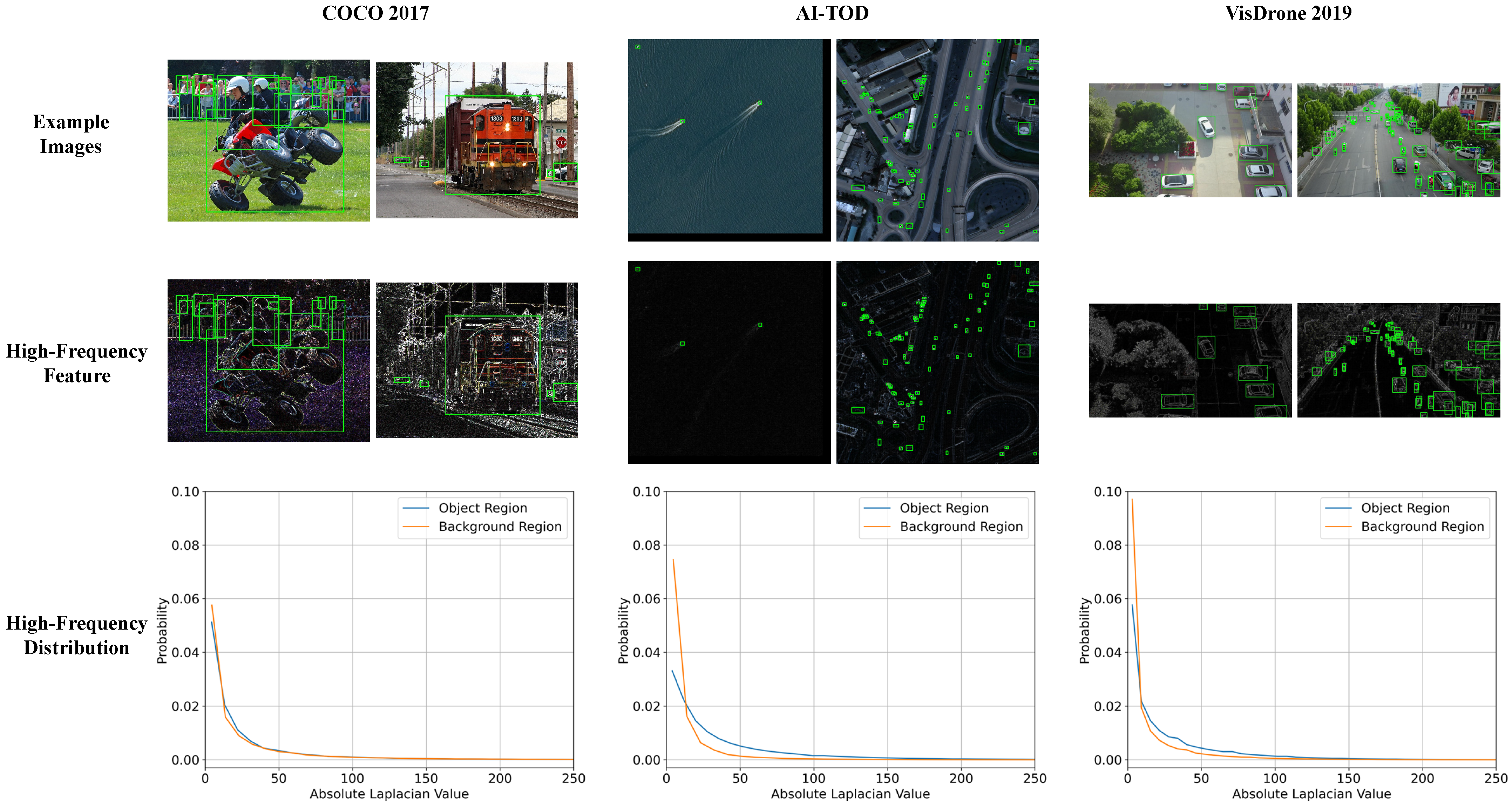
Figure 1.
Comparison of frequency component distributions in object and background regions between natural and remote sensing images. The object regions annotated in the ground truth labels are marked by green rectangular boxes. High-frequency features are extracted using the Laplacian operator. The high-frequency feature maps are obtained by extracting frequency-domain responses separately from the R, G, and B channels, where brighter colors indicate stronger high-frequency components. The frequency distribution plots are computed from grayscale images, and larger x-axis values correspond to higher-frequency features.
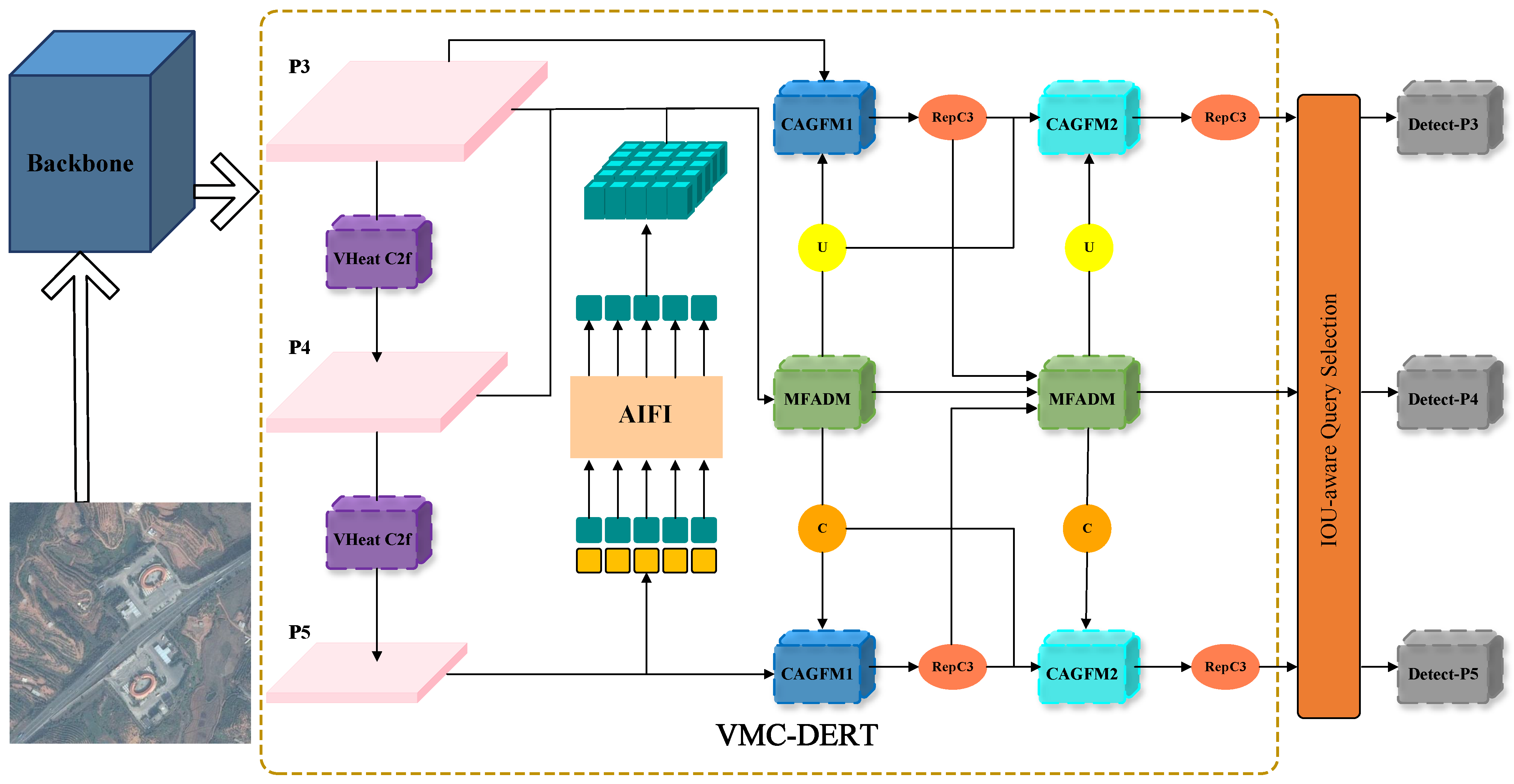
Figure 2.
The overall architecture of the proposed VMC-DETR framework consists mainly of three modules: the VHeat C2f module, which is based on visual heat conduction; the MFADM, a multi-scale feature aggregation distribution module; and the CAGFM, a contextual attention guided fusion module, where CAGFM1 refers to the dual-branch CAGFM and CAGFM2 refers to the triple-branch CAGFM. The remaining modules include U, which handles upsampling operations; C, responsible for downsampling using ADown [
46]; AIFI, an attention-based intrascale feature interaction module; and RepC3 [
14], designed for reparameterization convolution.
Figure 3.
Visual comparison of feature maps from traditional backbone networks (ResNet, C3, and C2f) and the proposed VHeat C2f backbone on aerial images from various categories and scenes. The colormap encodes the strength of feature responses, where yellow corresponds to high response values, often associated with salient texture or edge information, while dark green represents weaker responses. Variations in response strength allow for intuitive observation of how different backbone networks capture high-frequency features with varying levels of precision and accuracy.
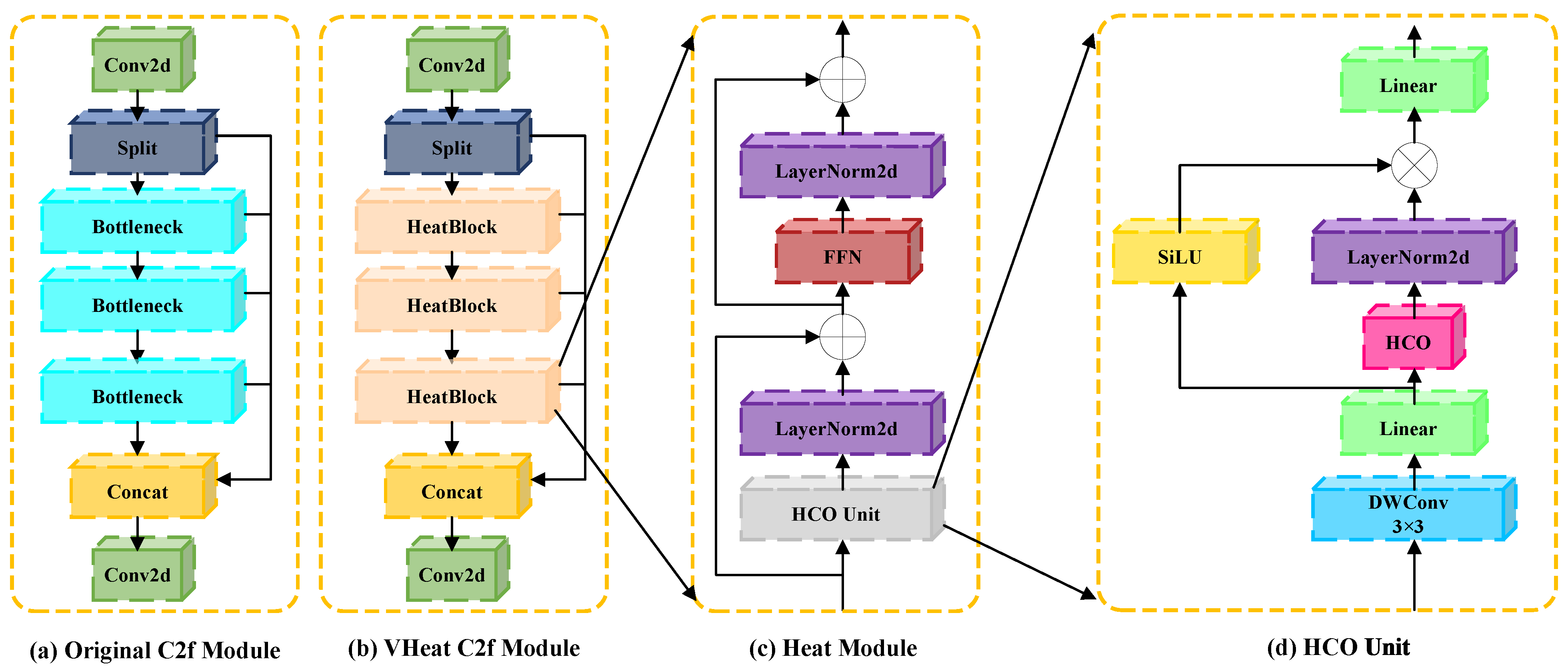
Figure 4.
Detailed architecture of the VHeat C2f module used in the backbone network. (a) Original C2f module, which consists of a convolutional layer, a split-branch structure, and three sequential Bottleneck blocks followed by concatenation. (b) Modified VHeat C2f module, where Bottleneck blocks are replaced with HeatBlocks to enhance high-frequency feature learning. (c) Heat Module, which introduces frequency-domain processing with residual connections and normalization layers. (d) HCO Unit, which performs the heat conduction operation using discrete cosine transforms, simulating spatial-frequency energy propagation. Here, ⊗ denotes the Hadamard product and ⊕ represents element-wise addition. HCO in (d) stands for Heat Conduction Operation.
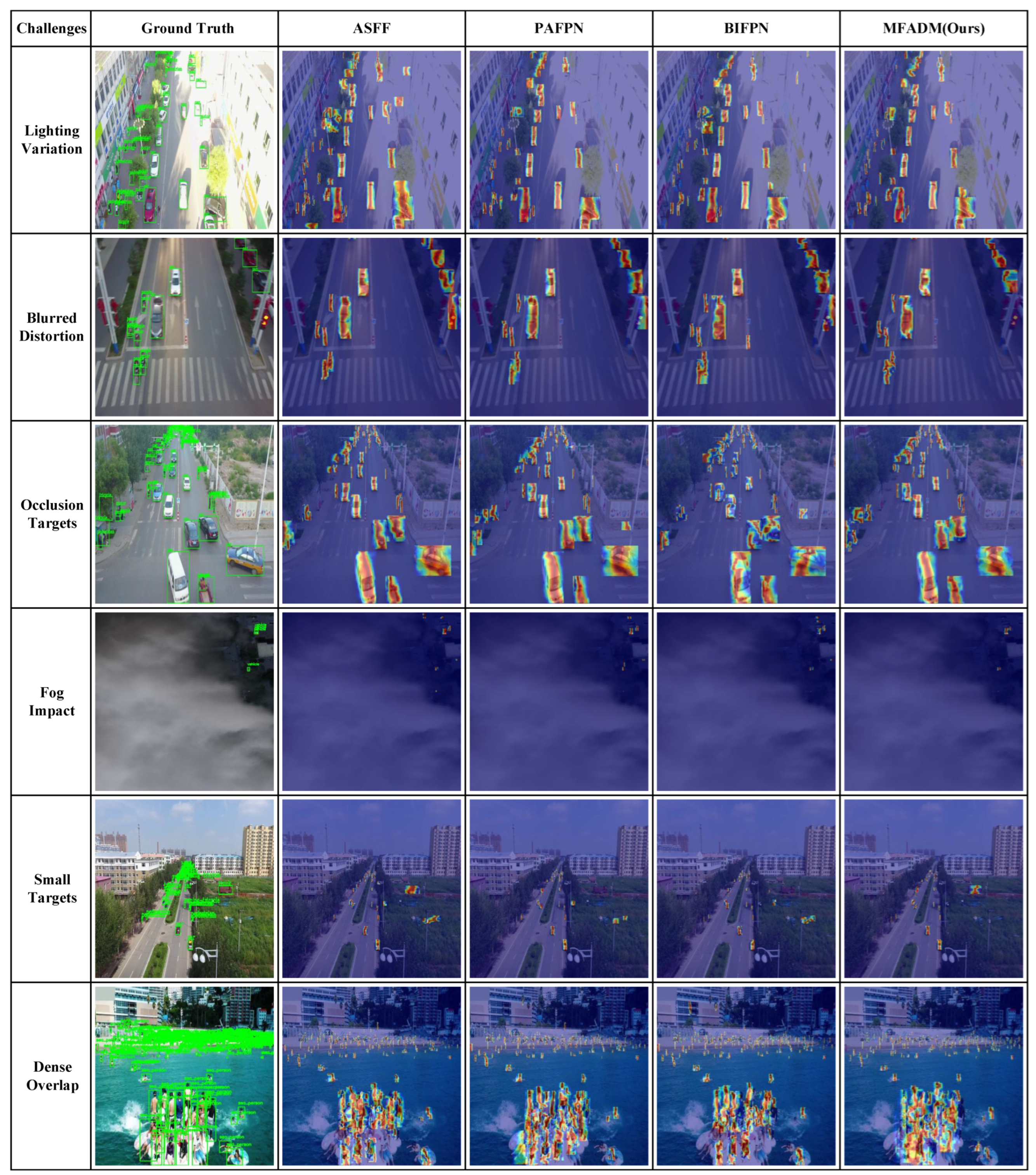
Figure 5.
Comparison of heatmap activations under typical challenges in aerial object detection using different multi-scale feature fusion methods, including ASFF, PAFPN, BIFPN, and the proposed MFADM. The colormap highlights feature response intensity, where red and yellow regions indicate strong attention and blue denotes weak response. The green bounding boxes in the Ground Truth column denote annotated object locations. Despite minor visual overlap, all target areas remain clearly identifiable and do not hinder scientific interpretation.
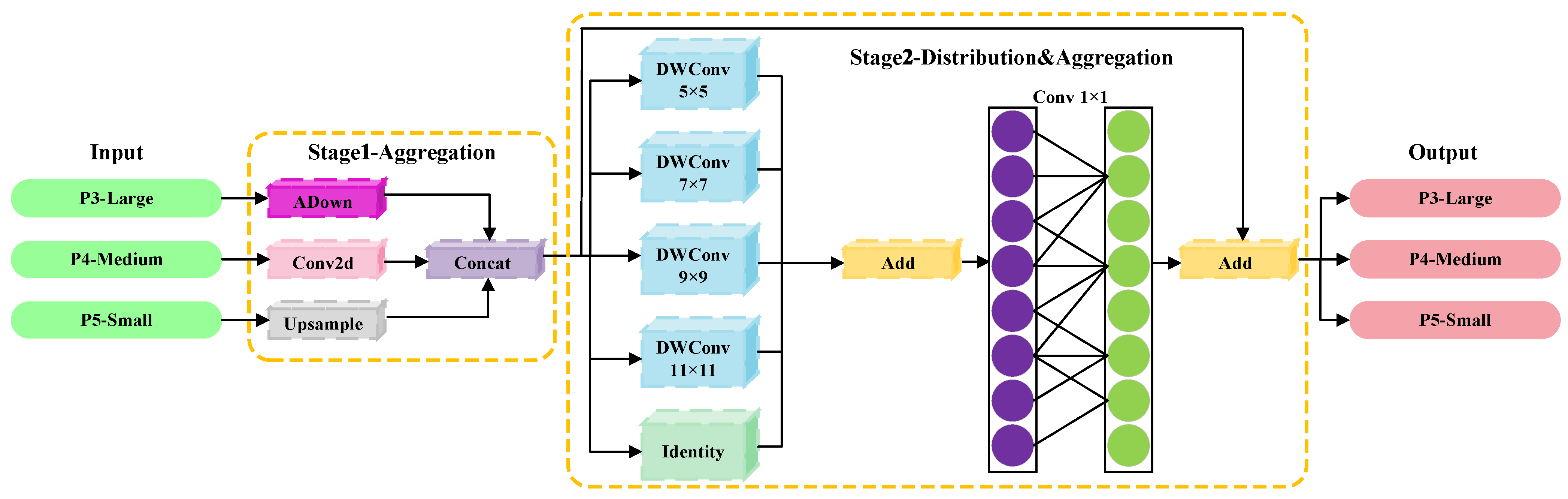
Figure 6.
The detailed process of the MFADM module: ADown denotes the downsampling module of YOLOv9, DWConv represents the depthwise convolution, and Identity refers to the identity mapping.
Figure 6.
The detailed process of the MFADM module: ADown denotes the downsampling module of YOLOv9, DWConv represents the depthwise convolution, and Identity refers to the identity mapping.
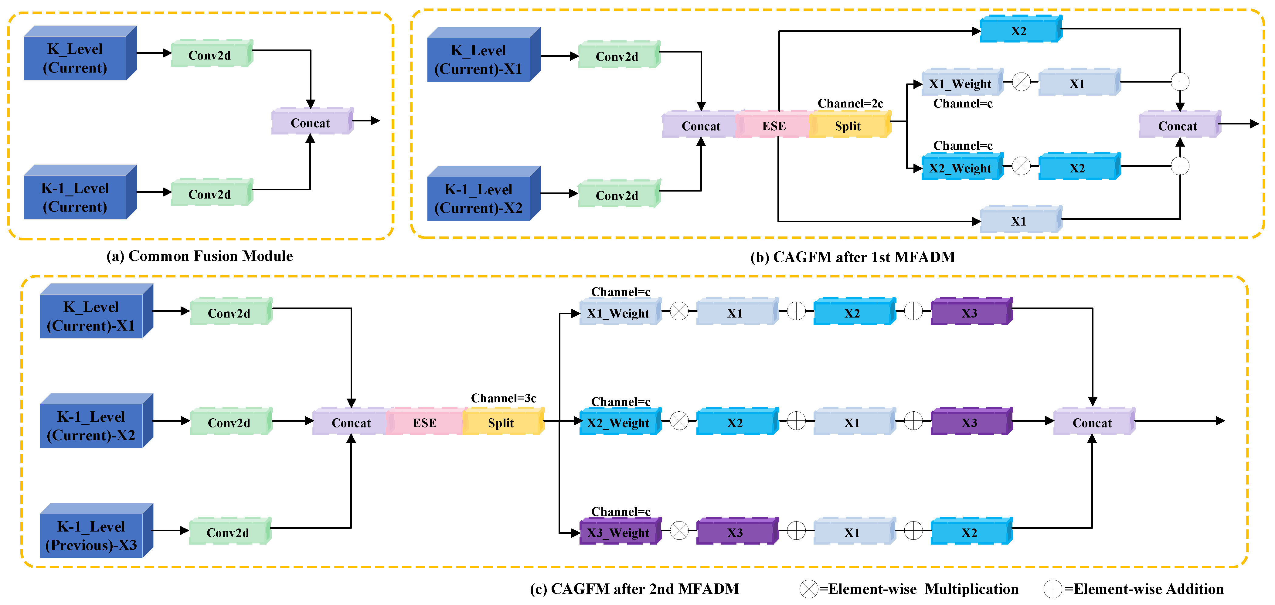
Figure 7.
Specific details of the CAGFM module implementation: ESE stands for the effective squeeze and extraction attention mechanism. (
a) Standard feature fusion operation, (
b) dual-branch CAGFM, (
c) triple-branch CAGFM.
,
, and
represent input feature maps from different scales or stages. The terms
,
, and
denote the channel-wise attention weights computed via the contextual attention mechanism (ESE [
56]), adjusting the contributions of each feature map in the fusion process.
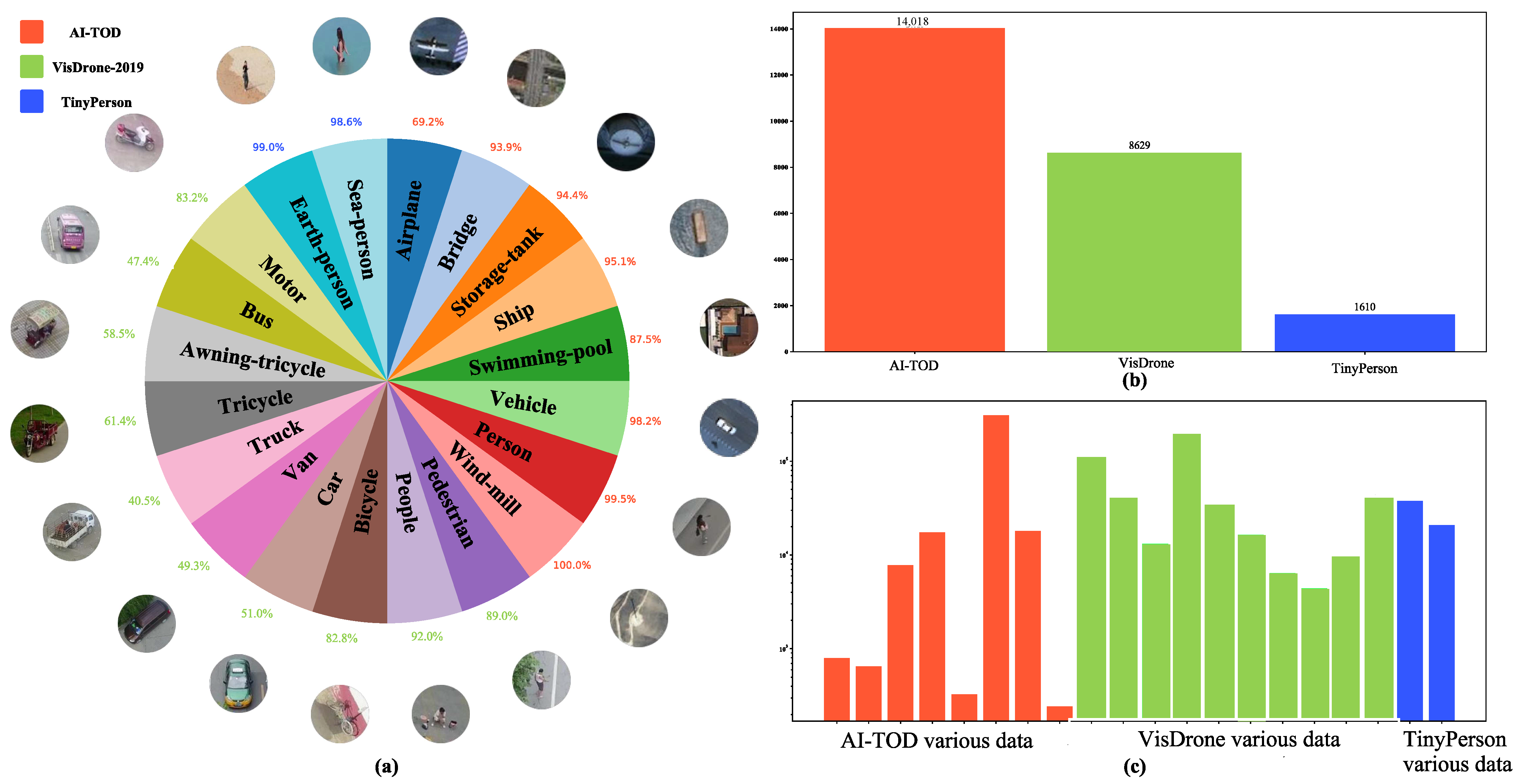
Figure 8.
(a) Object category names, image examples, and the proportion of small objects across the three datasets. (b) The number of images in each of the three datasets. (c) The number of instances for each object category across the three datasets.
Figure 8.
(a) Object category names, image examples, and the proportion of small objects across the three datasets. (b) The number of images in each of the three datasets. (c) The number of instances for each object category across the three datasets.
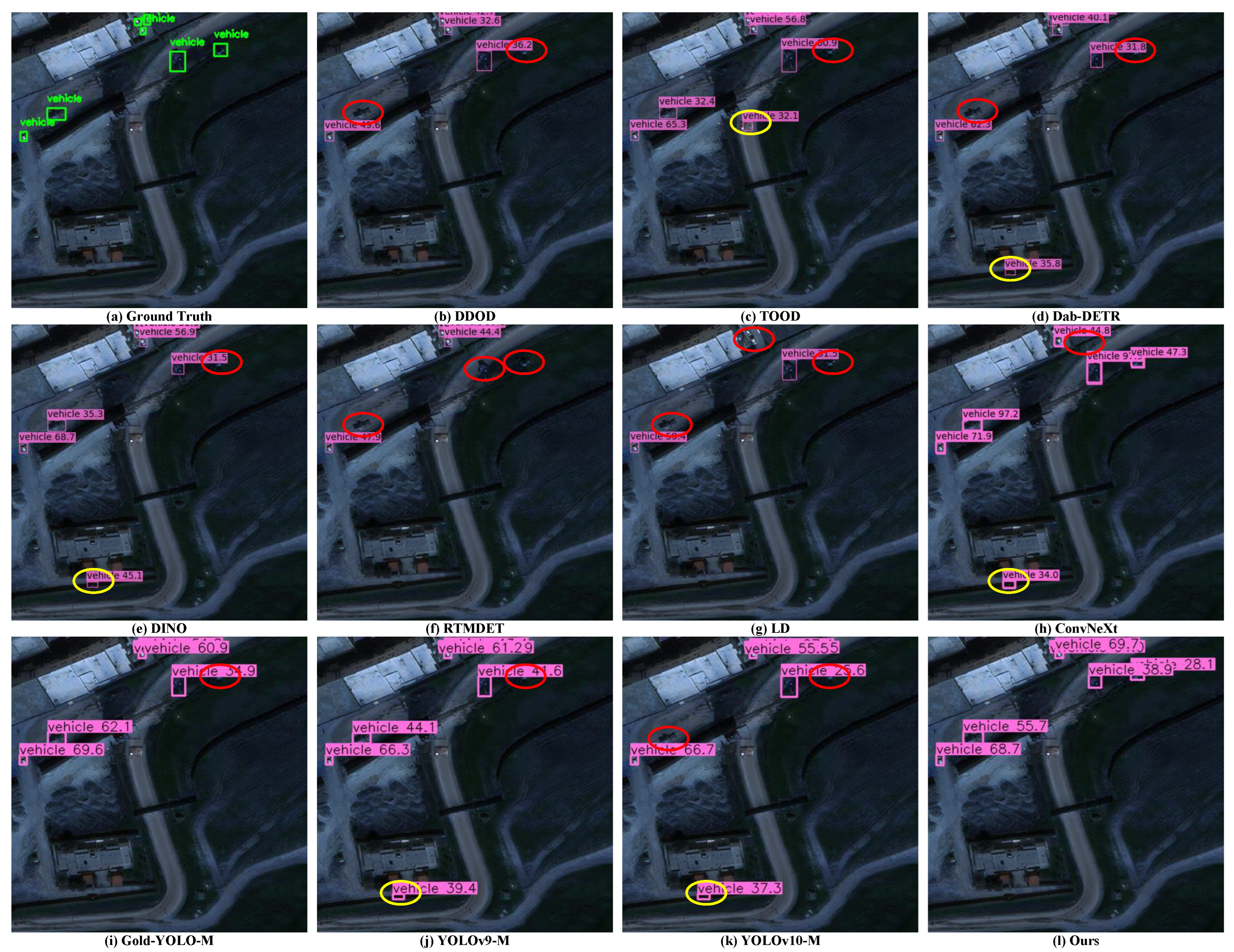
Figure 9.
Visualization of all comparison methods on the AI-TOD dataset. (a) shows the ground truth bounding boxes. (b–h) are detection results visualized using MMDetection version 3.3.0, while (i–l) are generated using Ultralytics version 8.0.201. Red circles highlight false positive detections, and yellow circles mark missed detections.
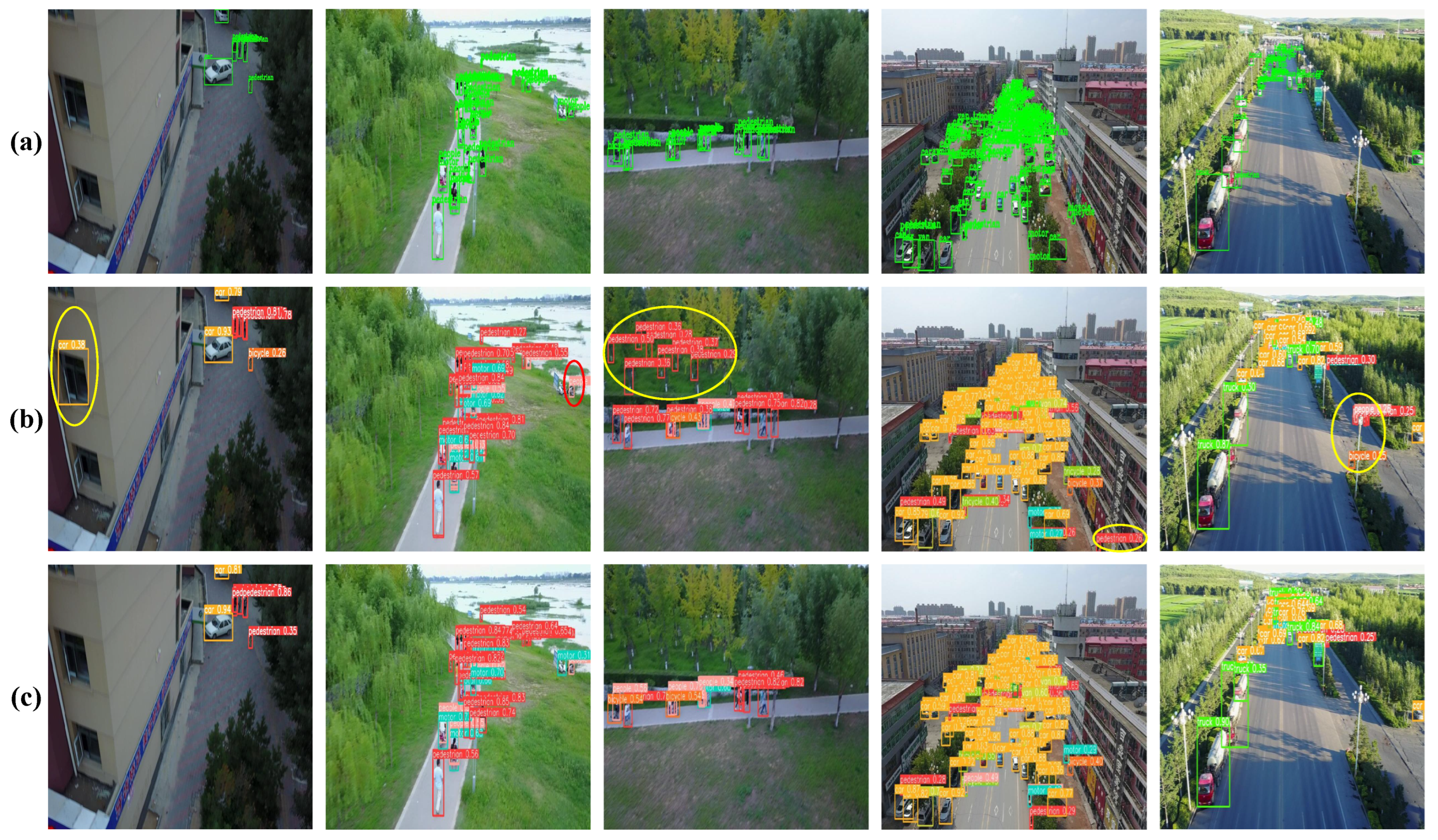
Figure 10.
Comparison of visualization effects with baseline methods on the VisDrone-2019 dataset, implemented using Ultralytics version 8.0.201. (a) shows the ground truth annotations, (b) presents detection results from the baseline model, and (c) displays the results of our proposed method. Yellow circles highlight missed detections or false classifications made by the baseline method.
Figure 11.
mAP curves from ablation experiments on the AI-TOD, VisDrone-2019, and TinyPerson datasets, showing the performance impact of each module.
Figure 11.
mAP curves from ablation experiments on the AI-TOD, VisDrone-2019, and TinyPerson datasets, showing the performance impact of each module.
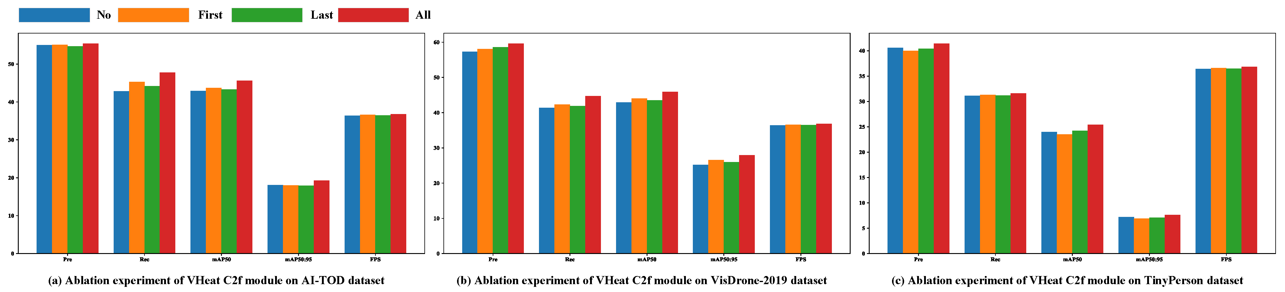
Figure 12.
Effect of varying frequency and placement of the VHeat C2f module across the AI-TOD, VisDrone-2019, and TinyPerson datasets. “First” indicates that the VHeat C2f module is used only between the P3 and P4 layers, “Last” indicates that it is used only between the P4 and P5 layers, “No” indicates that the standard C2f module is used in both locations, and “All” indicates that the VHeat C2f module is used in both locations.
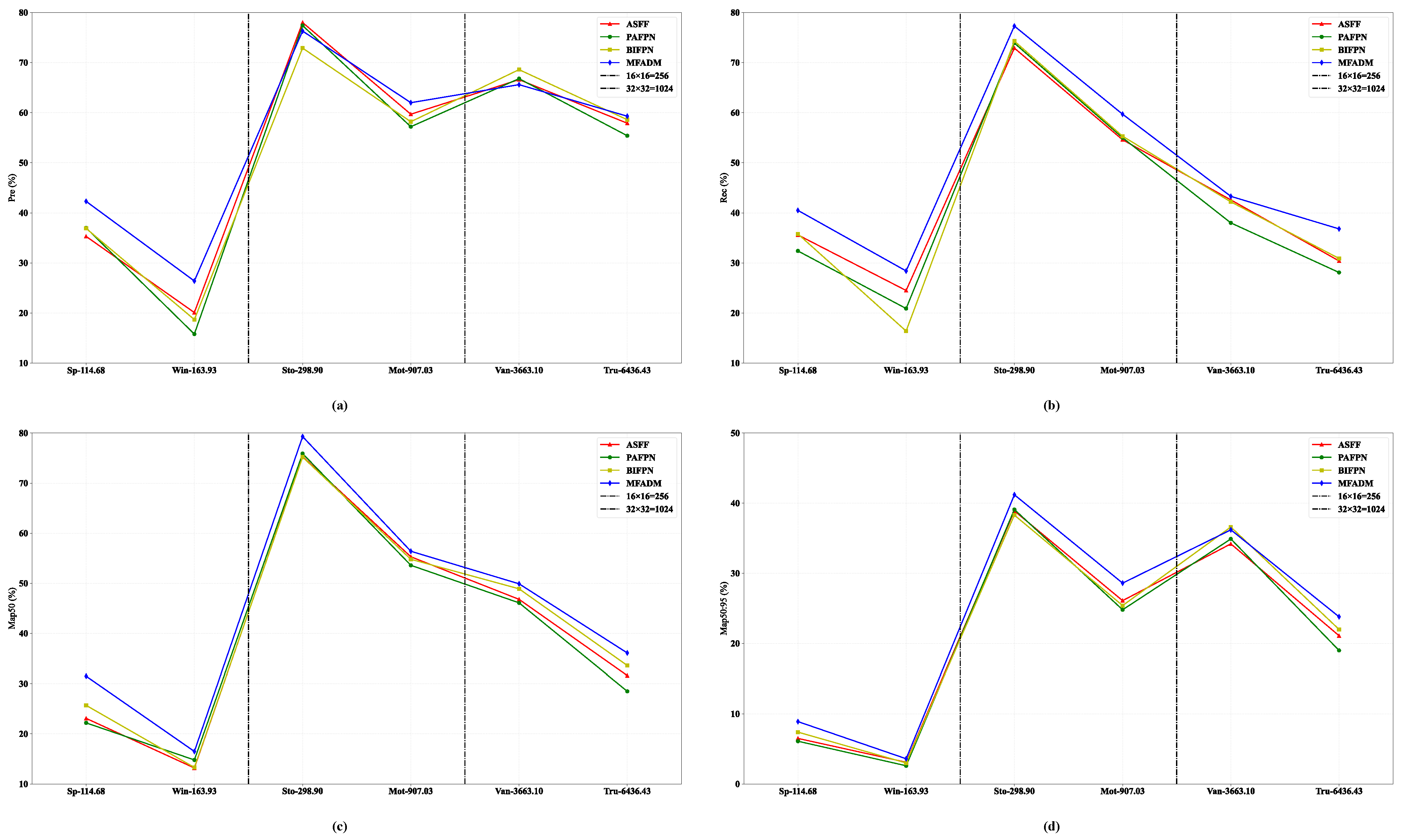
Figure 13.
The comparison between the proposed MFADM and classic multi-scale feature fusion strategies on aerial image object-detection datasets is presented. The vertical axes in (a), (b), (c), and (d) represent the performance metrics of Pre, Rec, mAP50, and mAP50:95, respectively, while the horizontal axes indicate the average area of object instances in pixels.
Figure 14.
Effect of different attention mechanisms in CAGFM on context-guided fusion, evaluated through ablation experiments across the AI-TOD, VisDrone-2019, and TinyPerson datasets. Higher Pre, Rec, mAP50, and mAP50:95 indicate greater model accuracy, higher FPS represents faster inference, and lower GFLOPs imply a more lightweight model.
Table 1.
The hyperparameters and their corresponding values used in the experiments. Adam denotes the adaptive moment estimation optimizer, and IoU represents intersection over union.
Table 1.
The hyperparameters and their corresponding values used in the experiments. Adam denotes the adaptive moment estimation optimizer, and IoU represents intersection over union.
| Hyperparameters | Values |
|---|
| Learning Rate | 0.0001 |
| Batch Size | 8 |
| Optimizer | Adam |
| Epochs | 150 |
| Input Image Size | 640 × 640 |
| Weight Decay | 0.0001 |
| Momentum | 0.9 |
| IoU Threshold | 0.7 |
Table 2.
Data augmentation techniques and their application ratios used in the experiment.
Table 2.
Data augmentation techniques and their application ratios used in the experiment.
| Data Augmentation | Ratios |
|---|
| Hue | 0.015 |
| Saturation | 0.7 |
| Value | 0.4 |
| Translate | 0.1 |
| Scale | 0.5 |
| Flip Left-Right | 0.5 |
Table 3.
Comparison experiments with current mainstream methods on the AI-TOD dataset. Each object category and mAP are expressed as percentages (%), IT represents the inference time for a single image (ms), and MU denotes peak memory usage during model runtime (MB). Bold numbers indicate the best results among all compared methods.
| Method | Air | Bri | Per | Shi | Sto | Swi | Veh | Win | mAP50 | mAP50:95 | FPS | GFLOPs | IT | MU |
|---|
| DDOD-R50 [60] | 28.8 | 9.3 | 14.3 | 50.6 | 52.4 | 0.1 | 48.4 | 0.0 | 25.5 | 10.9 | 32.2 | 111 | 29.4 | 371 |
| TOOD-R50 [61] | 35.8 | 31.0 | 20.0 | 57.6 | 56.2 | 10.9 | 51.2 | 10.6 | 34.2 | 14.9 | 28.6 | 124 | 35.0 | 365 |
| Dab-DETR-R50 [62] | 22.3 | 2.9 | 9.2 | 33.9 | 18.5 | 2.1 | 17.0 | 11.8 | 14.7 | 4.3 | 25.3 | 72.4 | 39.5 | 412 |
| DINO-R50 [63] | 45.4 | 48.0
| 29.7 | 65.8 | 74.9 | 10.9 | 62.4 | 16.0 | 44.1 | 15.5 | 19.8 | 179 | 50.5 | 437 |
| RTMDET-M [64] | 50.0 | 25.4 | 20.4 | 54.5 | 59.7 | 26.9 | 53.7 | 4.9 | 36.9 | 16.0 | 36.7 | 39.7 | 27.2 | 315 |
| LD-R50 [65] | 21.0 | 0.0 | 10.9 | 40.6 | 34.5 | 5.3 | 30.6 | 0.0 | 17.9 | 7.5 | 40.6 | 128 | 24.6 | 567 |
| ConvNeXt-R50 [66] | 48.0 | 33.1 | 12.5 | 42.0 | 33.4 | 15.6 | 33.3 | 7.7 | 28.2 | 12.4 | 27.8 | 189 | 36.0 | 1031 |
| Gold-YOLO-M [67] | 46.0 | 33.9 | 24.0 | 64.5 | 77.2 | 17.7 | 69.0 | 10.2 | 42.8 | 18.3 | 27.4 | 79.3 | 8.7 | 338 |
| YOLOv9-M [46] | 52.7 | 37.7 | 24.9 | 64.6 | 77.2 | 13.9 | 69.1 | 8.6 | 43.6 | 19.0 | 31.8 | 77.9 | 8.5 | 290 |
| YOLOv10-M [68] | 50.0 | 29.9 | 24.1 | 64.7 | 78.4 | 7.0 | 68.6 | 11.5 | 41.8 | 18.7 | 38.8 | 64.0 | 8.2 | 284 |
| Baseline [14] | 31.1 | 42.4 | 28.3 | 69.9 | 76.7 | 2.8 | 67.7 | 7.0 | 40.7 | 16.8 | 37.6 | 66.1 | 9.0 | 277 |
| Ours | 42.0 | 42.9 | 30.7 | 70.8 | 79.3 | 12.8 | 69.7 | 16.5 | 45.6 | 19.3 | 36.8 | 70.5 | 9.2 | 302 |
Table 4.
Comparison experiments with current mainstream methods on the VisDrone-2019 dataset. All values are expressed as percentages (%). Bold numbers indicate the best results for each metric across all methods.
Table 4.
Comparison experiments with current mainstream methods on the VisDrone-2019 dataset. All values are expressed as percentages (%). Bold numbers indicate the best results for each metric across all methods.
| Method | Year | Awn | Bic | Bus | Car | Mot | Ped | Peo | Tri | Tru | Van | mAP50 | mAP50:95 |
|---|
| DDOD-R50 | 2021 | 14.2 | 18.2 | 58.5 | 78.8 | 47.5 | 47.4 | 34.9 | 27.5 | 41.0 | 45.4 | 40.7 | 24.8 |
| TOOD-R50 | 2021 | 14.2 | 19.8 | 56.4 | 79.3 | 49.2 | 46.8 | 35.4 | 27.2 | 40.9 | 45.6 | 38.8 | 24.3 |
| Dab-DETR-R50 | 2022 | 15.3 | 12.7 | 57.5 | 66.7 | 26.2 | 21.4 | 14.3 | 19.7 | 39.3 | 38.2 | 31.1 | 15.5 |
| DINO-R50 | 2022 | 18.0 | 18.3 | 61.2 | 83.9 | 51.2 | 58.1 | 44.3 | 30.7 | 38.5 | 49.6 | 45.4 | 26.7 |
| RTMDET-M | 2022 | 14.6 | 12.1 | 56.1 | 75.2 | 40.4 | 34.2 | 28.3 | 25.1 | 36.3 | 41.4 | 36.4 | 21.5 |
| LD-R50 | 2022 | 7.6 | 5.1 | 29.6 | 68.4 | 24.5 | 33.5 | 18.3 | 12.9 | 21.7 | 31.3 | 25.3 | 14.7 |
| ConvNeXt-R50 | 2022 | 17.2 | 21.7 | 60.5 | 75.2 | 42.5 | 39.4 | 32.6 | 32.8 | 44.0 | 49.8 | 41.6 | 24.7 |
| Gold-YOLO-M | 2023 | 18.8 | 14.4 | 59.8 | 80.4 | 46.6 | 43.5 | 34.2 | 30.3 | 40.9 | 45.5 | 41.4 | 25.0 |
| YOLOv9-M | 2024 | 17.7 | 15.5 | 62.2 | 80.8 | 47.4 | 43.5 | 34.3 | 31.8 | 39.6 | 46.9 | 42.0 | 25.2 |
| YOLOv10-M | 2024 | 16.8 | 16.2 | 59.0 | 81.3 | 47.2 | 46.0 | 36.1 | 31.1 | 38.7 | 47.2 | 42.0 | 25.3 |
| Baseline | 2023 | 11.8 | 13.3 | 52.2 | 81.9 | 49.7 | 45.4 | 39.0 | 28.2 | 27.8 | 46.3 | 39.6 | 23.7 |
| Ours | - | 18.9
| 19.1 | 59.8 | 84.2 | 56.4 | 54.0 | 47.9 | 33.1 | 36.1 | 49.9 | 45.9 | 27.9 |
Table 5.
Comparison experiments with current mainstream methods on the TinyPerson dataset. All values are expressed as percentages (%). Bold numbers indicate the best performance for each metric across all methods.
Table 5.
Comparison experiments with current mainstream methods on the TinyPerson dataset. All values are expressed as percentages (%). Bold numbers indicate the best performance for each metric across all methods.
| Method | Ep | Sp | mAP50 | mAP50:95 |
|---|
| DDOD-R50 | 11.6 | 24.3 | 18.0 | 5.9 |
| TOOD-R50 | 13.0 | 26.1 | 19.5 | 6.1 |
| Dab-DETR-R50 | 3.2 | 10.1 | 6.6 | 1.8 |
| DINO-R50 | 18.0 | 30.5 | 24.3 | 6.8 |
| RTMDET-M | 14.6 | 26.3 | 20.4 | 6.7 |
| LD-R50 | 5.9 | 12.7 | 9.3 | 2.7 |
| ConvNeXt-R50 | 7.1 | 16.2 | 11.6 | 3.6 |
| Gold-YOLO-M | 18.3 | 30.1 | 24.2 | 6.9 |
| YOLOv9-M | 17.1 | 29.0 | 23.1 | 7.2 |
| YOLOv10-M | 15.0 | 23.1 | 19.0 | 5.7 |
| Baseline | 17.9 | 26.1 | 22.0 | 6.6 |
| Ours | 19.3
| 31.5 | 25.4 | 7.5 |
Table 6.
Ablation experiment results on the AI-TOD dataset. All values are expressed as percentages (%). Bold numbers indicate the best performance for each metric across all variants.
Table 6.
Ablation experiment results on the AI-TOD dataset. All values are expressed as percentages (%). Bold numbers indicate the best performance for each metric across all variants.
| Method | Pre | Rec | mAP50 | mAP50:95 |
|---|
| Baseline | 47.9 | 42.0 | 40.7 | 16.8 |
| VHeat C2f | 54.1 | 44.1 | 42.2 | 18.1 |
| CAGFM | 52.7 | 43.4 | 41.0 | 17.1 |
| MFADM | 47.9 | 45.2 | 41.8 | 17.3 |
| VHeat C2f + CAGFM | 61.3
| 42.4 | 42.5 | 18.1 |
| VHeat C2f +
MFADM | 51.2 | 46.5 | 43.4 | 17.7 |
| MFADM+CAGFM | 55.0 | 42.8 | 42.9 | 18.1 |
| Ours | 55.4 | 47.8 | 45.6 | 19.3 |
Table 7.
Ablation experiment results on the VisDrone-2019 dataset. All values are expressed as percentages (%). Bold numbers indicate the best performance for each metric across all ablation variants.
Table 7.
Ablation experiment results on the VisDrone-2019 dataset. All values are expressed as percentages (%). Bold numbers indicate the best performance for each metric across all ablation variants.
| Method | Pre | Rec | mAP50 | mAP50:95 |
|---|
| Baseline | 53.7 | 37.9 | 39.6 | 23.7 |
| VHeat C2f | 56.4 | 40.4 | 42.4 | 25.5 |
| CAGFM | 55.2 | 40.1 | 41.2 | 24.6 |
| MFADM | 55.0 | 38.2 | 40.0 | 23.8 |
| VHeat C2f + CAGFM | 56.5 | 41.5 | 43.1 | 25.9 |
| VHeat C2f + MFADM | 57.5 | 41.9 | 43.4 | 26.3 |
| MFADM+CAGFM | 57.3 | 41.4 | 42.9 | 25.2 |
| Ours | 59.6
| 44.7 | 45.9 | 27.9 |
Table 8.
Ablation experiment results on the TinyPerson dataset. All values are expressed as percentages (%). Bold numbers indicate the best performance in each column.
Table 8.
Ablation experiment results on the TinyPerson dataset. All values are expressed as percentages (%). Bold numbers indicate the best performance in each column.
| Method | Pre | Rec | mAP50 | mAP50:95 |
|---|
| Baseline | 37.6 | 28.9 | 22.0 | 6.6 |
| VHeat C2f | 41.4 | 30.2 | 23.8 | 6.9 |
| CAGFM | 39.4 | 30.0 | 23.2 | 6.9 |
| MFADM | 37.6 | 31.5 | 23.9 | 7.2 |
| VHeat C2f + CAGFM | 40.9 | 31.5 | 24.2 | 7.3 |
| VHeat C2f +MFADM | 42.6
| 30.1 | 24.4 | 7.4 |
| MFADM+CAGFM | 40.6 | 31.1 | 24.0 | 7.2 |
| Ours | 41.4 | 31.6 | 25.4 | 7.6 |
Table 9.
Ablation experiments on the AI-TOD, VisDrone-2019, and TinyPerson datasets using different downsampling methods in the first feature aggregation stage of the MFADM module, including Interpolation, AvgPool2d, Conv2d, and ADown. Bold numbers indicate the best performance in each column.
Table 9.
Ablation experiments on the AI-TOD, VisDrone-2019, and TinyPerson datasets using different downsampling methods in the first feature aggregation stage of the MFADM module, including Interpolation, AvgPool2d, Conv2d, and ADown. Bold numbers indicate the best performance in each column.
| Method | FPS | AI-TOD | VisDrone-2019 | TinyPerson |
|---|
| Pre | Rec | mAP50 | mAP50:95 | Pre | Rec | mAP50 | mAP50:95 | Pre | Rec | mAP50 | mAP50:95 |
|---|
| Interpolation | 35.2 | 54.2 | 47.9 | 44.5 | 18.3 | 58.5 | 43.6 | 44.6 | 26.9 | 39.6 | 30.1 | 23.2 | 6.8 |
| AvgPool2d | 37.9
| 53.9 | 47.7 | 44.3 | 18.2 | 58.7 | 43.5 | 44.9 | 27.2 | 39.8 | 30.1 | 23.9 | 7.1 |
| Conv2d | 36.5 | 54.6 | 48.2 | 45.1 | 18.8 | 58.9 | 44.1 | 45.1 | 27.2 | 40.7 | 32.0 | 24.6 | 7.2 |
| ADown [46] | 36.8 | 55.4 | 47.8 | 45.6 | 19.3 | 59.6 | 44.7 | 45.9 | 27.9 | 41.4 | 31.6 | 25.4 | 7.6 |
Table 10.
Ablation experiments on three datasets for different numbers, strides, and sizes of deep convolutional kernels used in the distribution operation in the third stage of the MFADM module. Bold numbers indicate the best performance in each column.
Table 10.
Ablation experiments on three datasets for different numbers, strides, and sizes of deep convolutional kernels used in the distribution operation in the third stage of the MFADM module. Bold numbers indicate the best performance in each column.
| Design | Numbers | Strides | FPS | GFLOPs | AI-TOD | VisDrone-2019 | TinyPerson |
|---|
| Pre | Rec | mAP50 | Pre | Rec | mAP50 | Pre | Rec | mAP50 |
|---|
| (5, 7, 9) | 3 | 2 | 37.1 | 68.9 | 55.5 | 45.8 | 43.7 | 58.6 | 42.2 | 44.1 | 39.3 | 29.2 | 23.5 |
| (7, 9, 11) | 3 | 2 | 37.0 | 69.6 | 55.1 | 45.9 | 45.3 | 59.0 | 42.8 | 44.8 | 40.0 | 29.2 | 24.1 |
| (9, 11, 13) | 3 | 2 | 36.8 | 70.3 | 53.7 | 45.1 | 43.2 | 59.0 | 44.9 | 45.5 | 37.8 | 28.9 | 23.4 |
| (3, 7, 11, 15) | 4 | 4 | 36.8 | 70.8 | 53.8 | 43.3 | 43.3 | 58.7 | 42.2 | 44.2 | 36.1 | 29.9 | 22.7 |
| (3, 5, 7, 9) | 4 | 2 | 36.9 | 69.9 | 53.4 | 45.7 | 43.5 | 59.3 | 43.1 | 44.5 | 38.3 | 29.7 | 23.3 |
| (7, 9, 11, 13) | 4 | 2 | 36.7 | 71.0 | 55.6
| 45.3 | 45.5 | 60.2 | 42.9 | 45.0 | 41.3 | 30.0 | 25.2 |
| (9, 11, 13, 15) | 4 | 2 | 36.6 | 71.6 | 54.0 | 45.4 | 44.1 | 58.4 | 41.8 | 43.5 | 38.6 | 29.5 | 24.0 |
| (5, 7, 9, 11)-Ours | 4 | 2 | 36.8 | 70.5 | 55.4 | 47.8 | 45.6 | 59.6 | 44.7 | 45.9 | 41.4 | 31.6 | 25.4 |


