1. Introduction
The rapid development of urban infrastructure, particularly large–scale transportation hubs and complex underground facilities, has driven the advancement of ultra–deep and clustered engineering. Accurately detecting underground cavities in such deep engineering environments remains a significant challenge in the field of geophysical exploration. Traditional ground–based geophysical methods are limited in resolution and detection depth, particularly when targeting features that are deeply buried or small–scale. In contrast, cross–hole radar tomography offers a promising alternative. It enables the accurate identification and characterization of cavity structures, such as their spatial distribution, shape, and fill materials, at significant depths, thereby providing an effective tool for detecting potential geological hazards in complex deep–earth environments.
Conventional cross–hole radar imaging techniques are primarily based on tomography, which relies on the travel time and amplitude of electromagnetic (EM) waves as influenced by the dielectric properties of the subsurface medium [
1]. However, traditional ray–based tomography methods face significant resolution limitations in heterogeneous media because of wave scattering [
2]. To improve imaging quality, full–waveform inversion (FWI) was introduced into ground–penetrating– radar (GPR) detection, offering more detailed subsurface reconstructions [
3,
4]. However, FWI demands a good initial model and substantial computational resources. Therefore, traditional methods face significant challenges in terms of stability, accuracy, and computational efficiency.
With recent advancements in computing power, deep learning (DL) has demonstrated considerable potential in geophysical imaging tasks, enabling the modeling of complex nonlinear relationships between inputs and outputs [
5]. Several studies have applied DL to GPR–based detection [
6,
7]. For instance, Dinh et al. (2018) developed an algorithm that combines traditional image processing with deep convolutional neural networks (CNNs) to detect reinforcing bars in GPR images [
8] automatically. Lei et al. (2019) integrated the Faster R–CNN framework with data augmentation to identify hyperbolic features in GPR data [
9]. Similarly, DL approaches have also been applied to cross–hole radar. Zhang et al. (2023) developed an inversion framework based on a generative adversarial network (GAN) that converts radar images directly into two–dimensional subsurface structures [
10]. Pongrac et al. (2023) introduced a supervised CNN–based method to estimate soil moisture using cross–hole radar records [
11]. Liu et al. (2024) proposed a UNET–based approach for high–resolution slowness tomography from cross–hole radar data [
12]. However, most of these studies rely on multi–channel radar profiles for the training of deep networks, which may lead to many problems and limitations. For example: (1) high computational cost—generating a large number of training datasets using finite-difference time-domain (FDTD) simulations is computationally intensive [
13]; (2) huge data scale—due to the deep drilling depth (exceeding 50 m), a multi-channel GPR profile may contain upwards of tens of thousands of traces, containing excessive information, which will slow the training of the DL model [
11]; (3) the difficulty of feature extraction—the waveform features in multi-channel radar profiles are highly susceptible to environmental interference, complicating feature extraction [
10]; and (4) poor generalization capability—discrepancies between simulated and real-world data—due to differences in wavelets, instrumentation, and subsurface conditions—create a “simulation-to-reality” gap that reduces model performance in practical scenarios [
14]. In summary, current DL-based methods for deep underground cavity imaging using cross-hole radar face substantial limitations in cost-effectiveness, feature robustness, and, most importantly, generalization to real–world conditions. To address these limitations, we conducted our research.
In 2015, Ronneberger et al. [
15] proposed the “U” –shaped neural network to realize image feature segmentation and “end–to–end” learning. Based on the specific requirements of cross–hole radar travel-time imaging in this paper, the UNET architecture demonstrates three theoretical advantages: (1) Image–to–image mapping capability—UNET’s encoder–decoder structure with symmetric feature extraction and reconstruction perfectly aligns with our need for “travel-time fingerprint to velocity model” conversion. (2) Learning potential—U-–Net has demonstrated exceptional data efficiency in semantic segmentation tasks based on a small number of samples. This characteristic directly addresses our core challenge of limited real–world cross–hole radar data and scarce labeled samples. (3) Physical model integration—UNET’s simple and straightforward architecture facilitates the integration of physical constraints, allowing for the straightforward incorporation of enhancement modules to improve physical consistency [
16,
17,
18].
Based on the advantages of the UNET architecture, we propose a novel imaging method that utilizes a UNET model enhanced with transfer learning (TL). This approach adapts pre–trained models to new tasks using limited data [
19]. The input features consist of travel–time fingerprints, a newly defined concept that compresses cross–hole radar records into structured 2D matrices. Initially, we proposed innovative construction methods for cavity models alongside their corresponding 2D travel–time fingerprints. Using this framework, datasets of cavity models paired with their travel–time fingerprints are generated. Subsequently, a UNET is pretrained to establish the mapping relationship between travel–time fingerprints and velocity models. To improve the generalization of real–world engineering applications, TL is employed to fine–tune the pre–trained network. Finally, numerical experiments validate the effectiveness and accuracy of the proposed method, while successful field tests conducted at a highway foundation site highlight its practical value for geophysical detection in complex environments.
2. Methodology
In DL applications, constructing a high–quality and diverse dataset is crucial for effective model training and robust generalization. Although DL is adept at learning intricate nonlinear relationships between inputs and outputs, its success is heavily reliant on the availability of large–scale, representative datasets. However, acquiring sufficient cross–hole radar data from real–world scenarios presents challenges due to limited site access and the considerable variability in geological conditions.
To address this issue, this section introduces methods for generating synthetic datasets, including the construction of cavity models and the generation of corresponding two–dimensional (2D) travel–time fingerprints. Subsequently, a modified UNET architecture is applied to map the travel–time fingerprints to subsurface velocity models, leveraging UNET’s strong feature extraction and skip–connection capabilities.
2.1. Cavity Model Construction
2.1.1. Irregular Cavity Generation Method
To accurately simulate the complex and irregular cavity geometries commonly found in subsurface environments, we propose a novel cavity generation algorithm that employs dynamic random boundary evolution. This methodology constructs complex cavities by expanding the upper and lower boundaries using a controlled stochastic walk.
Step 1: Cavity Parameters Initialization
The number of cavities is randomly determined, and the computational domain is defined with dimensions . Each time, random parameters and are generated, and represent the X–axis and Y–axis coordinates of the cavity’s center point, respectively. The half–width of each cavity is also set randomly as . Boundary conditions are applied to ensure that cavities do not extend beyond the limits of the model.
Step 2: Directional Sequences Generation
Each X–coordinate corresponds to a random direction sequence (the value of the direction sequence is −1 or 1). A corresponding sequence is obtained by flipping the signs of . These antipodal sequences govern asymmetric boundary development through coordinated vertical displacement.
Step 3: Dynamic Boundary Expansion
Fix the position of an X–coordinate and calculate the variation in the upper and lower boundaries at each
x–position with the width, adhering to the following formula:
where
and
denote the upper and lower boundary positions at each vertical slice.
Step 4: Cavity Filling and Model Construction
At each vertical slice (x–position), the area from to in the y direction is filled with materials that have distinct dielectric properties, simulating the presence of cavities. This process creates geometries with jagged or sawtooth–like features, effectively matching field cavities.
This method generates a ‘stacked layers’ effect, with each vertical slice exhibiting independently varying heights and irregular cavities, effectively enriching the variability and realism of the training datasets.
2.1.2. Generation of Cavity Model Datasets
Utilizing the methodology delineated in
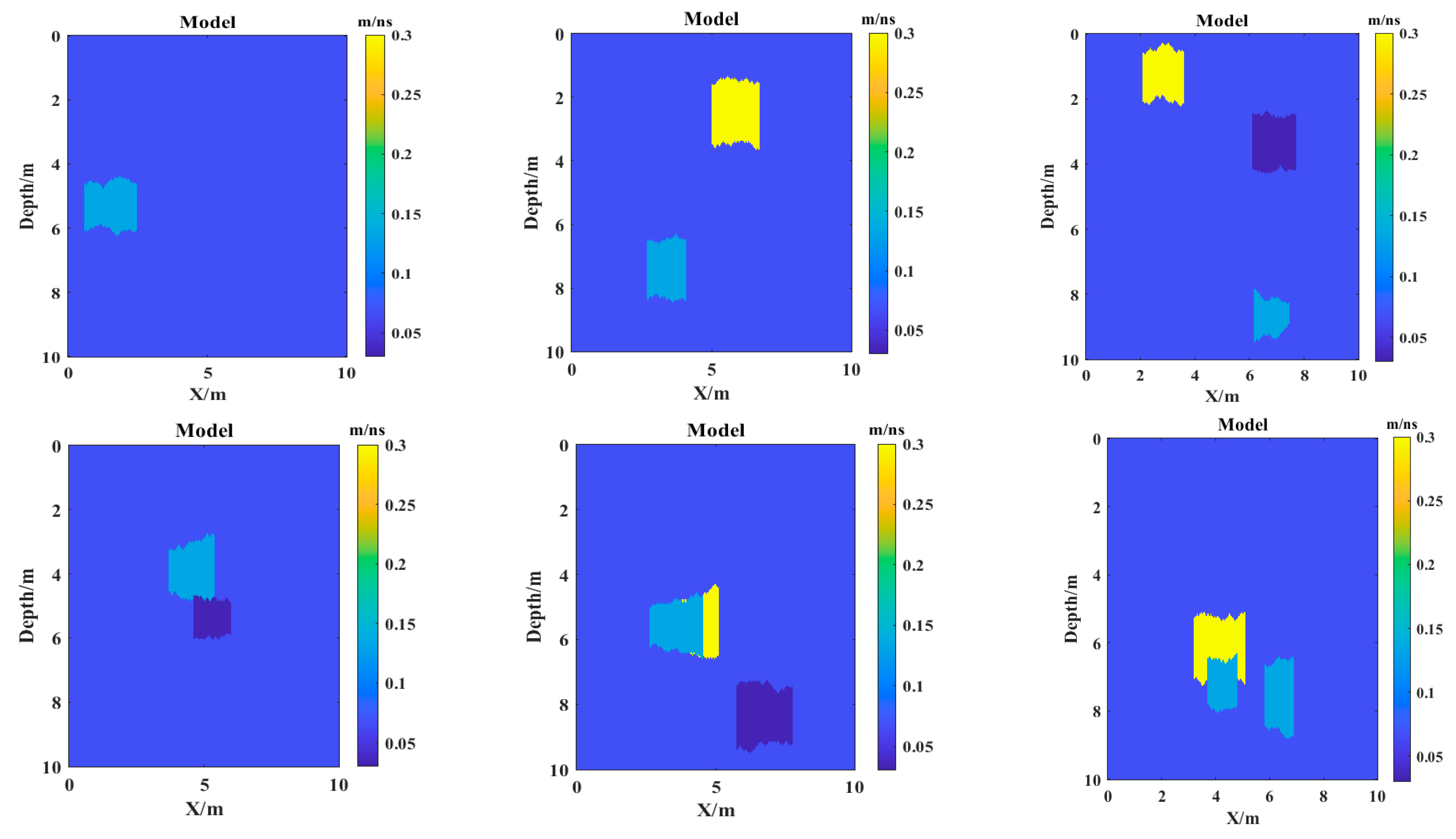
Section 2.1.1, a comprehensive set of 1500 synthetic half–space models, each with a size of 10 m × 10 m, was systematically generated. Within each model, the presence of one and three randomly situated irregular cavities was incorporated to enhance variability. A representative example of one such model is illustrated in
Figure 1.
To accurately simulate realistic geological conditions, the cavities were filled with typical materials such as air, water, and mud, each possessing distinctly different dielectric constants of 1, 81, and 5, respectively. The background medium was designated with a relative permittivity of 20.
Table 1 provides a summary of the EM properties of all materials involved.
The corresponding EM wave propagation velocities are calculated using the relationship derived from Maxwell’s equations [
20]
where
is the speed of light in vacuum (3 ×
m/s), and
is the material’s relative permittivity. Under the assumption of weak conductivity and nonmagnetic materials (
), Equation (2) provides a valid approximation of EM wave velocity in geological media.
By applying Equation (2), we convert the permittivity distributions into velocity models that reflect both the geometries of cavities and the properties of materials. These velocity models serve as output labels for training the DL network.
Figure 2 illustrates six representative examples of these constructed velocity models.
2.2. The Construction Method of Travel–Time Fingerprints
2.2.1. Construction Method of Travel–Time Fingerprints
The complexity of wave propagation in cross–hole radar surveys can be effectively reduced by using first–arrival travel times. We present a DL–based framework that leverages this physical compression by establishing travel–time fingerprints—unique identifiers that encode subsurface structural information through differential arrival patterns.
This study employs the fast sweeping method (FSM) to estimate radar wave travel times efficiently. The FSM, developed initially to solve first–order nonlinear hyperbolic partial differential equations, has been widely applied in seismic wave modeling [
21]. It enables the fast computation of first–arrival travel times without solving the full wave equation. The travel–time field
satisfies the Eikonal equation
where
denotes the slowness field, and
is the local wave velocity.
To systematically validate the FSM, a synthetic 2D velocity model is presented in
Figure 3a. The transmitter is located at (0 m, 5.4 m) along the left domain boundary, and 80–element receiver points are deployed along
x = 9.0 m with vertical sampling from
z = 1.1 m to 9.0 m (Δ
z = 0.1 m). FSM is subsequently used to compute the travel–time curve, which is then overlaid on the radar waveform in
Figure 3b. The curve aligns well with the actual radar record, validating the accuracy and reliability of the FSM.
Therefore, the FSM was used to calculate the travel time of every transmitter–receiver pair. All the computed travel–time data were organized into a matrix, where each row corresponds to a transmitter and each column corresponds to a receiver. The element at position (
i,
j) represents the travel time from the
ith transmitter to the
jth receiver. This original travel–time matrix was then normalized to the range [
1,
2], resulting in the final travel–time fingerprint.
2.2.2. Generation of Travel–Time Fingerprint Datasets
Using the cavity models from
Section 2.1.2 and the method described in
Section 2.2.1, a total of 1500 travel–time fingerprints were generated. As illustrated in
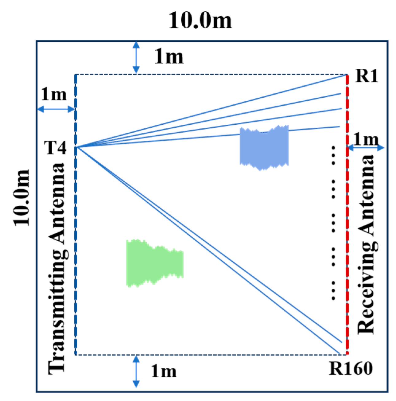
Figure 4a, the transmitting points are fixed on the left side of each model, with coordinates ranging from (1.0 m, 1.05 m) to (1.0 m, 9.0 m), spaced at intervals of 0.05 m. The receiving points are located on the right side of the model, spanning from (9.0 m, 1.05 m) to (9.0 m, 9.0 m), with a spacing of 0.05 m. This setup yields 160 transmitting points and 160 receiving points, forming 25,600 transmitter–receiver pairs for each model. The construction method of the two–dimensional travel–time fingerprint is illustrated in
Figure 4b. As shown in
Figure 4, taking the fourth transmitting point as an example, the first to the 160th receiving points receive signals in sequence and the corresponding travel–time data are calculated. Then, all the data are respectively filled into the fourth column of the matrix. The arrows in
Figure 4 represent the data filling process.
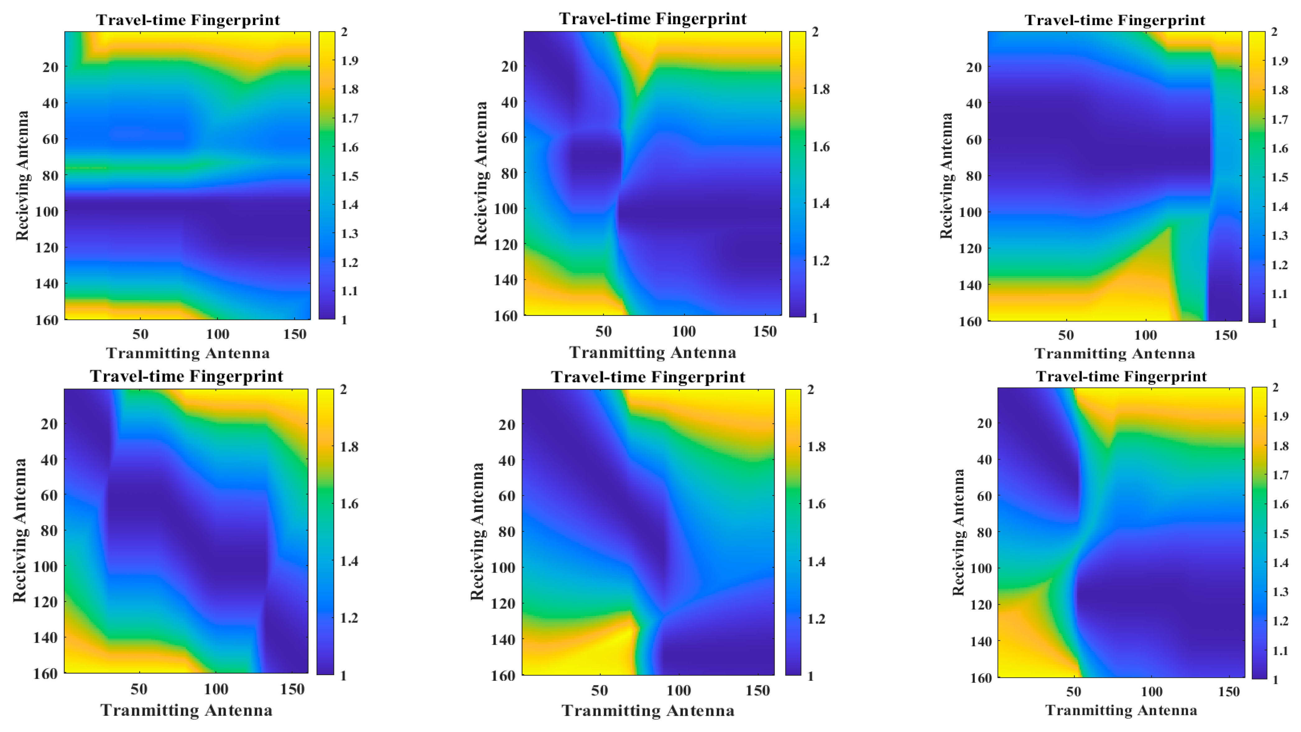
Figure 5 shows six representative travel–time fingerprints corresponding to the velocity models in
Figure 2. The distinct spatial differences observed across these fingerprints reflect their sensitivity to the underlying cavity configurations, confirming their utility as input features for training DL models to identify and localize subsurface anomalies.
2.3. Construction of the Pre–Trained UNET
To perform the inverse mapping from travel–time fingerprints to velocity models, a modified UNET architecture is employed, as illustrated in
Figure 6. This architecture consists of an encoder, a decoder, and skip connections. The encoder includes five feature extraction blocks, with four blocks performing down–sampling operations and one utilizes a max pooling layer. A batch normalization layer was incorporated at each stage of the down–sampling process. In the decoder, four up–sampling blocks are followed by a 1×1 convolutional layer with a ReLU activation function. Skip connections were included to reduce information loss and contribute to the recovery of the cavity boundary during the encoding process. Lastly, the transformation of image size was achieved through linear interpolation. To mitigate the risk of overfitting, a dropout rate of 0.2 was set.
The model was pre–trained using synthetic datasets derived from
Section 2.1.2 and
Section 2.2.2. Of the entire dataset, 90% was allocated for training, while the remaining 10% was reserved for testing. The travel–time fingerprints serve as the input to the network, with the corresponding velocity models serving as the output. The primary training parameters for pre–training are outlined in
Table 2.
Since the task is a regression problem, the mean squared error (
MSE) loss function is employed to evaluate model performance:
where
is the ground truth value of sample
i,
is the predicted value of sample
i, and
N is the total number of samples.
During the training process, the
MSE loss demonstrates a clear downward trend as shown in
Figure 7. Initially, there was rapid convergence in the early stages, followed by a gradual stabilization as the number of iterations increased. At the end of the training process, the training loss decreased significantly from 10.5208 to 0.1538, which is the minimal value.
To evaluate the model’s performance, three random samples were selected from the test set. Each travel–time fingerprint was input into the pre–trained UNET, and the predicted velocity models derived from the UNET were compared to the ground truth. The results are shown in
Figure 8.
In
Figure 8, the predicted models (right column) exhibit strong consistency with the real models (middle column), effectively recovering the shape, location, and extent of the underground cavities, which verifies the effectiveness of the pre–trained UNET.
3. Application and Discussion
Significant discrepancies frequently arose between synthetic training datasets and real–world field data, due to variations in wavelet characteristics, instrument responses, and complexities inherent in subsurface conditions. These divergences impede the direct application of models trained exclusively through simulation in practical engineering.
To improve the engineering applicability of the proposed method, a small set of field–inspired datasets was constructed to represent the target domain. A TL strategy was then employed, wherein the pre–trained UNET model was fine–tuned using the limited target domain data from the target domain, resulting in a retrained UNET. Finally, the effectiveness of this model was evaluated using actual field–scale synthetic datasets to validate its performance in more realistic geological conditions.
3.1. Transfer Learning and Retraining on Field–Scale Data
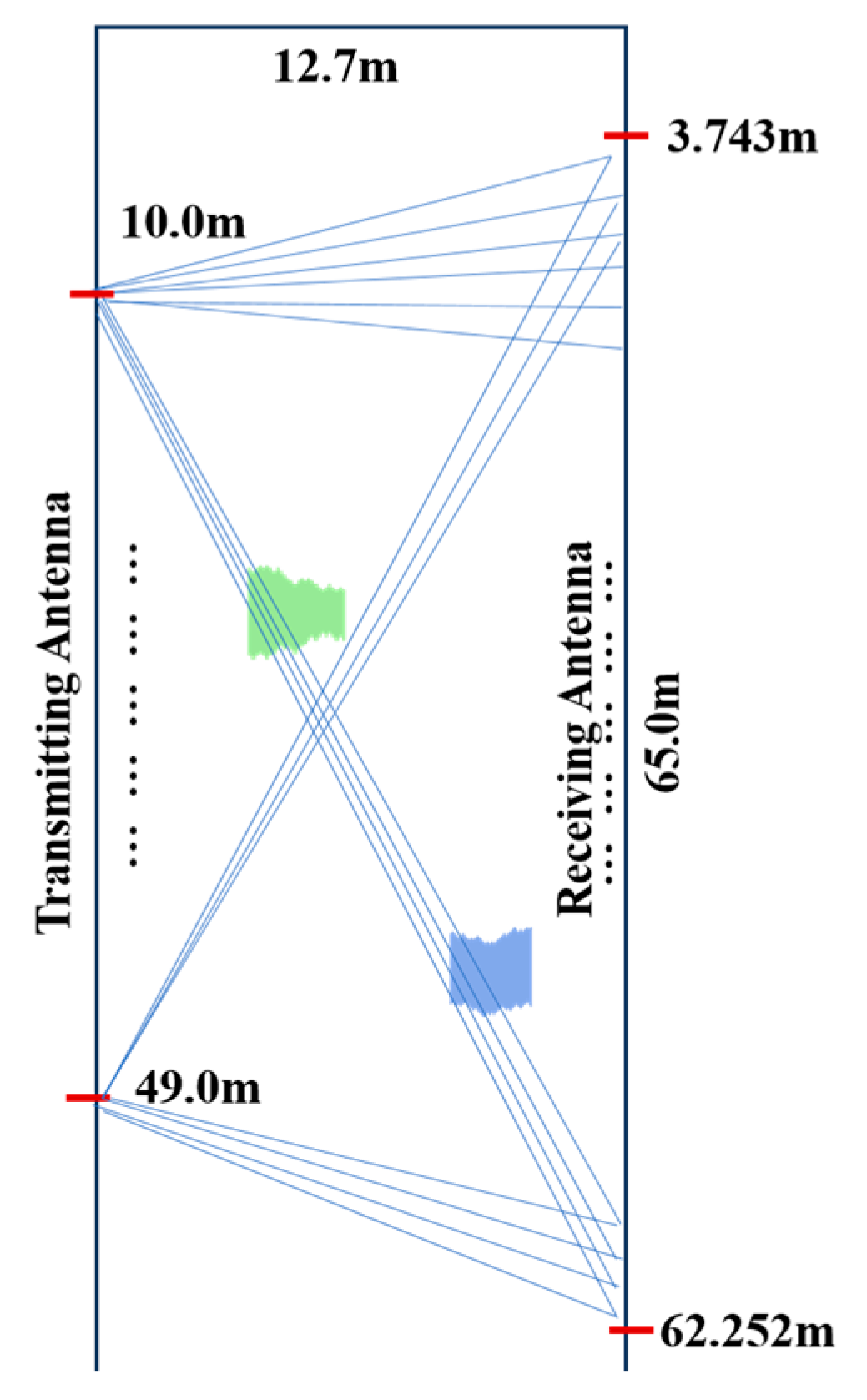
To validate the engineering applicability of TL, we developed an extensive velocity model dataset (62.25 m × 12.7 m,
Figure 9) within the target domain. This model retains the irregular cavity generation methodology detailed in
Section 2.1.1 and effectively simulates field–scale subsurface spatial structures under realistic geological conditions. This was achieved through strategic parameterization, with a relative dielectric constant of 9 assigned to the background medium.
The corresponding velocity distributions were derived using Equation (2) from
Section 2.1.2, producing a set of field–scale velocity models. As illustrated in
Figure 9, the antenna layout within the target domain is specified as follows: Transmitting antennas are positioned along the left boundary and are distributed between depths of 10 m to 49 m at 1 m intervals, yielding a total of 40 transmitters. Meanwhile, receiving antennas are fixed along the right boundary, spanning from 3.743 m to 62.252 m, with a spacing of 0.197 m, which corresponds to 298 receivers. Based on this antenna configuration, travel–time fingerprints were generated using the methodology outlined in
Section 2.2.1, adapted for the scale of the new model.
Based on the target domain dataset, a TL strategy was applied to fine–tune the previously pre–trained UNET model, thereby enhancing the engineering applicability of the network. Initially, the pre–trained UNET model was loaded. Following that, specific layers were frozen, while the remaining layers were updated to fine–tune during TL process.
The training parameters are detailed in
Table 3. The evaluation of the training process utilizes the MSE loss function. As illustrated in
Figure 10, both training and testing losses demonstrate a clear downward trend, indicating successful adaptation. Notably, the training loss decreased from 6.941 to 0.4879, highlighting effective learning, even with a limited amount of new data.
To assess the performance of the fine–tuned UNET in the target domain, three fingerprint–velocity model pairs were randomly selected from the test set. These fingerprints were fed into the retrained model, and the resulting predictions are shown in
Figure 11.
In
Figure 11, the predicted models successfully reconstruct the shape, location, and spatial extent of underground cavities, showing strong agreement with the true models. This confirms that the fine–tuned UNET has effectively generalized to the target domain.
3.2. Engineering Application
To further validate the engineering applicability and practical effectiveness of the proposed method, it was applied to a real–world expressway construction project in Guizhou Province, China. The project area featured complex geological conditions, and multiple sets of cross–hole radar data had already been acquired.
This section selects a representative borehole dataset from the project for demonstration. The proposed deep learning–based travel–time imaging method was applied to the dataset to identify and visualize subsurface anomalies.
3.2.1. Project Background
The study area is situated near the Pingtang Special Bridge, a part of the Yuqing–Anlong Expressway (specifically, the Pingtang–Luodian section). Cross–hole radar data were collected using a RAMAC radar system with 100 MHz borehole antennas, manufactured by MALA Geoscience (Solna, Sweden).
Field–acquired radar data underwent standard preprocessing steps, including DC drift removal, static correction, AGC gain adjustment, and bandpass filtering. The calculation steps for processing the field data are shown in
Figure 12.
3.2.2. Case Study: Borehole Pair ZK113–ZK99
A total of 3830 ray paths were generated between borehole ZK113 (acting as the transmitter) and borehole ZK99 (serving as the receiver), with a borehole spacing of 12.7 m. The layout reflects the settings of the synthetic target domain settings: transmitting points comprise 40 positions, ranging from 10 m to 59 m in 1 m intervals in ZK113; the receiving points encompass 298 positions, spanning from 3.743 m to 62.252 m at 0.197 m intervals in ZK99.
Figure 13 shows the raw radar record for ZK113–ZK99, which has undergone preprocessing according to the flowchart illustrated in
Figure 12. As shown in
Figure 14a, the corresponding travel–time fingerprints for these field data were obtained using the data processing flow outlined in
Figure 12. This travel–time fingerprint, shown in
Figure 14a, is then input into the fine–tuned UNET model to produce the predicted model shown in
Figure 14b. In
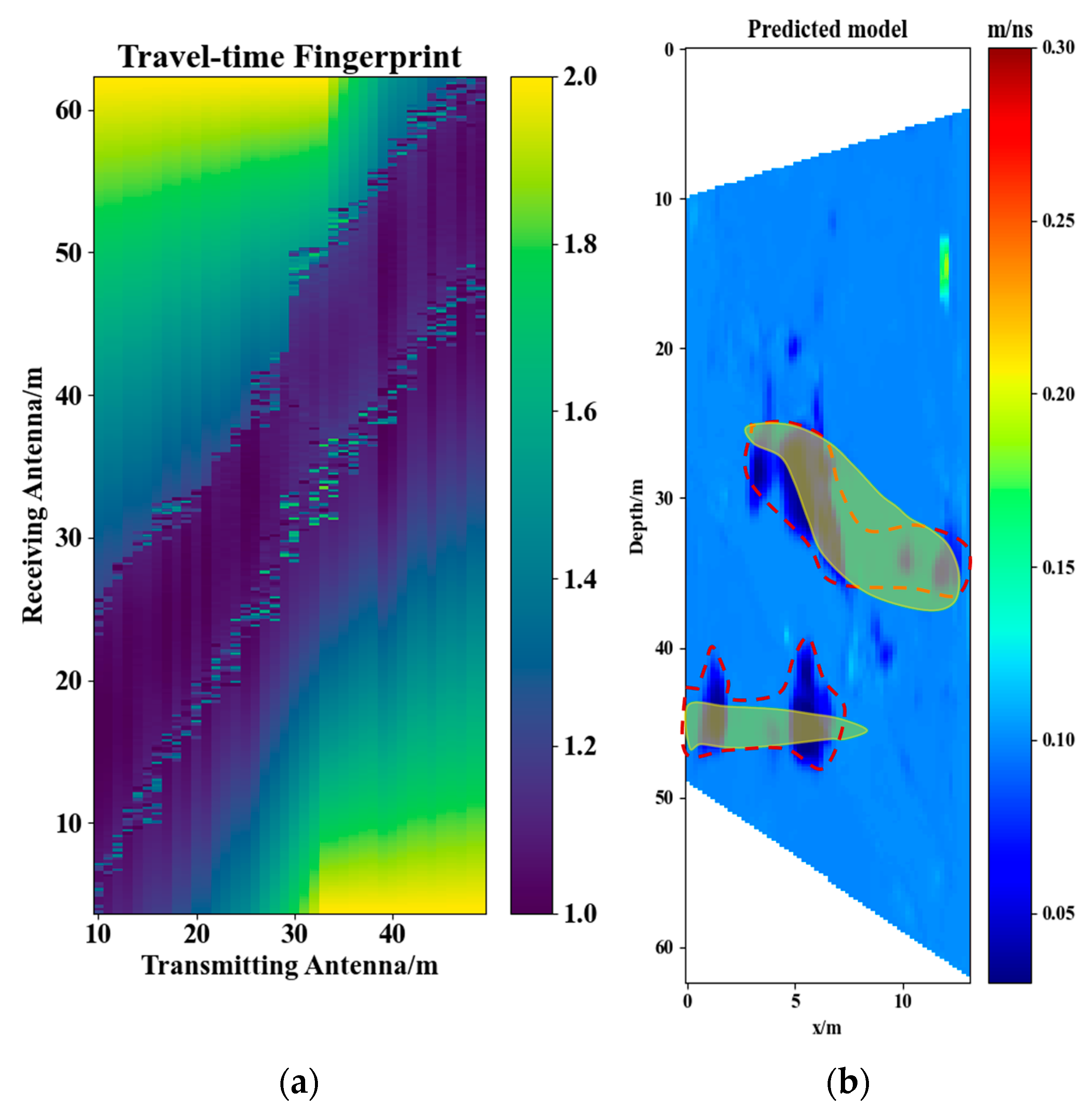
Figure 14b, the anomalies highlighted in the red dotted areas represent results obtained through the proposed method, while the regions marked in yellow indicate cavity areas identified through geological interpretation via traditional methods. Two notable low–velocity anomalies—likely indicative of water–filled or clay–filled cavities—are clearly visible and emphasized in the red–dotted line areas: (1) spanning depth from 24 m to 39 m; horizontal extent from 2.5 m to 12.7 m from ZK113; (2) ranging from 42 m to 47 m in depth with a horizontal extent from 0 m to 8 m from ZK113.
Figure 15a presents the tomography imaging result obtained through the traditional tomography method. It reveals a weak velocity contrast and low spatial resolution, which make it difficult to clearly define the boundaries of cavities. In
Figure 15b, the geological interpretation derived from the tomography results is displayed. The abnormal cavities indicated in this figure are also highlighted in yellow in
Figure 14b, enabling the comparison of the results from both methods. According to the geophysical report of the CT result of this project: (1) In the section of the hole ZK113 ranging from a depth of 26.3 m to 39.5 m, the EM waves at a horizontal distance area of 3.2 m to 12.7 m from ZK113 to ZK99 exhibit characteristics of high absorption and low wave velocity. This phenomenon is speculated to indicate a semi–filled cavity, which contains water and a small amount of crushed stone soil at the bottom. (2) In the section of hole ZK113 ranging from a depth of 47.3 m to 46.9 m, the EM waves within a horizontal distance of 0.0 m to 8.0 m from ZK113 to ZK99 show high absorption and low wave velocity [
22]. The results and comparative analysis of
Figure 14 and
Figure 15 indicate a strong consistency in the cavity positions identified by both methods.
Figure 15b presents the geological interpretation and data from a verification borehole ZK106, situated 8 m along the alignment from ZK113 toward ZK99. The verification process revealed the presence of cavities at depths ranging from 24.5 m to 32.6 m and from 41.8 m to 43.6 m, which aligns well with the abnormal locations shown in
Figure 14b. The results from borehole ZK106 confirm the existence of two underground cavities between borehole pairs ZK113 and ZK99, substantiating the effectiveness of the proposed method.
The cavity prediction result in
Figure 14b was compared and analyzed with the tomography imaging result in
Figure 15. In
Figure 14b, the distribution and shape of underground low–speed cavities are clearly visible. Although the tomography result in
Figure 15a also identify the anomaly zones, they lack the intuitive visual clarity found in
Figure 14b, making geological interpretation challenging. In contrast, the proposed method offers enhanced visualization of the cavity shapes and extents, thereby facilitating a more profound understanding and informed decision–making in engineering.
In conclusion, the field–scale application of the proposed method demonstrates several key advantages: (1) accuracy—the imaging results closely align with traditional interpretations and physical borehole validation, verifying the method’s reliability; (2) visual clarity—the predicted models deliver high–resolution, interpretable outputs, simplifying the detection and delineation of subsurface anomalies for engineers; and (3) efficiency—following the completion of transfer learning, the inference speed for processing field data is significantly increased, providing considerable benefits to practical engineering workflows.
4. Conclusions
This study introduces an innovative DL–based subsurface cavity imaging method using cross–hole radar. The approach features a unique framework comprising travel–time fingerprints and a TL–enhanced UNET architecture. The travel–time fingerprint construction method converts cross–hole radar measurements into structured inputs that capture essential spatial propagation features, establishing the foundation for accurate underground imaging.
A pre–trained UNET model has been developed to establish the relationship between travel–time fingerprints and subsurface velocity structures. To address domain shifts between simulated and field data, transfer learning was employed to fine–tune the model using limited field–scale travel–time fingerprints, significantly improving its adaptability and accuracy in complex geological environments.
Numerical simulations and field applications, including field–scale case studies from a highway construction site in Guizhou Province, demonstrate the method’s precision, robustness, and practical feasibility. In comparison to conventional inversion techniques, the proposed approach exhibits enhanced interpretability and computational efficiency, facilitating the effective detection and delineation of deep subsurface cavities.
The methodology presented in this paper has undergone preliminary verification through numerical experiments and engineering applications; however, its practical implementation requires careful consideration. Furthermore, its applicability in various engineering scenarios requires additional testing and optimization. In practical engineering surveys, subsurface structures frequently demonstrate significant complexity with heterogeneous media distributions, which places heightened demands on the adaptability and stability of detection methods. Although the proposed approach has demonstrated impressive imaging performance under typical geological conditions, systematic validation across multiple practical engineering projects remains essential for broader applications. By accumulating field data from diverse geological settings (e.g., karst development zones, fracture zones, and multi–layer aquifers), we can optimize algorithm parameters further and refine network architecture design. These enhancements will improve the method’s adaptability and stability in various complex detection scenarios, ultimately providing more reliable technical support for engineering geological investigations.
Author Contributions
Conceptualization, H.C. and Y.Z.; methodology, H.C.; validation, H.C.; data curation, H.C. and K.F.; writing—original draft preparation, H.C.; writing—review and editing, H.C. and Y.Z.; funding acquisition, Y.Z. All authors have read and agreed to the published version of the manuscript.
Funding
This work was supported by the National Key R&D Program of China under Grant 2023YFC3009300.
Data Availability Statement
Data will be made available on request.
Conflicts of Interest
Author Kunwei Feng was employed by the company Guizhou Transportation Planning Survey & Design Academe Co., Ltd. The remaining authors declare that the research was conducted in the absence of any commercial or financial relationships that could be construed as a potential conflict of interest.
References
- Hanafy, S.; al Hagrey, S.A. Ground-penetrating radar tomography for soil-moisture heterogeneity. Geophysics 2006, 71, K9–K18. [Google Scholar] [CrossRef]
- Williamson, P.R. A guide to the limits of resolution imposed by scattering in ray tomography. Geophysics 1991, 56, 202–207. [Google Scholar] [CrossRef]
- Ernst, J.R.; Green, A.G.; Maurer, H.; Holliger, K. Application of a new 2D time-domain full-waveform inversion scheme to crosshole radar data. Geophysics 2007, 72, J53–J64. [Google Scholar] [CrossRef]
- Kuroda, S.; Takeuchi, M.; Kim, H.J. Full-waveform inversion algorithm for interpreting crosshole radar data: A theoretical approach. Geosci. J. 2007, 11, 211–217. [Google Scholar] [CrossRef]
- Zhu, J.-Y.; Park, T.; Isola, P.; Efros, A.A. Unpaired Image-to-Image Translation Using Cycle-Consistent Adversarial Networks. In Proceedings of the 2017 IEEE International Conference on Computer Vision (ICCV), Venice, Italy, 22–29 October 2017; pp. 2242–2251. [Google Scholar]
- Liu, B.; Ren, Y.; Liu, H.; Xu, H.; Wang, Z.; Cohn, A.G.; Jiang, P. GPRInvNet: Deep Learning-Based Ground Penetrating Radar Data Inversion for Tunnel Lining. IEEE Trans. Geosci. Remote Sens. 2021, 59, 8305–8325. [Google Scholar] [CrossRef]
- Ji, Y.; Zhang, F.; Wang, J.; Wang, Z.; Jiang, P.; Liu, H.; Sui, Q. Deep Neural Network-Based Permittivity Inversions for Ground Penetrating Radar Data. IEEE Sens. J. 2021, 21, 8172–8183. [Google Scholar] [CrossRef]
- Dinh, K.; Gucunski, N.; Duong, T.H. An algorithm for automatic localization and detection of rebars from GPR data of concrete bridge decks. Autom. Constr. 2018, 89, 292–298. [Google Scholar] [CrossRef]
- Lei, W.; Hou, F.; Xi, J.; Tan, Q.; Xu, M.; Jiang, X.; Liu, G.; Gu, Q. Automatic hyperbola detection and fitting in GPR B-scan image. Autom. Constr. 2019, 106, 102839. [Google Scholar] [CrossRef]
- Zhang, D.; Wang, Z.; Qin, H.; Geng, T.; Pan, S. GAN-Based Inversion of Crosshole GPR Data to Characterize Subsurface Structures. Remote Sens. 2023, 15, 3650. [Google Scholar] [CrossRef]
- Pongrac, B.; Gleich, D.; Malajner, M.; Sarjaš, A. Cross-Hole GPR for Soil Moisture Estimation Using Deep Learning. Remote Sens. 2023, 15, 2397. [Google Scholar] [CrossRef]
- Liu, X.; Liu, S.; Tian, S.; Zhao, Q.; Lu, Q.; Wang, K. Slowness High-Resolution Tomography of Cross-Hole Radar Based on Deep Learning. IEEE Geosci. Remote Sens. Lett. 2024, 21, 3000505. [Google Scholar] [CrossRef]
- Warren, C.; Giannopoulos, A.; Giannakis, I. gprMax: Open source software to simulate electromagnetic wave propagation for Ground Penetrating Radar. Comput. Phys. Commun. 2016, 209, 163–170. [Google Scholar] [CrossRef]
- Tong, Z.; Gao, J.; Yuan, D. Advances of deep learning applications in ground-penetrating radar: A survey. Constr. Build. Mater. 2020, 258, 120371. [Google Scholar] [CrossRef]
- Ronneberger, O.; Fischer, P.; Brox, T. U-Net: Convolutional Networks for Biomedical Image Segmentation. In Medical Image Computing and Computer-Assisted Intervention—MICCAI 2015, Proceedings of the Medical Image Computing and Computer-Assisted Intervention, Munich, Germany, 5–9 October 2015; Springer: Cham, Switzerland, 2015. [Google Scholar]
- Berezsky, O.; Pitsun, O.; Derysh, B.; Pazdriy, I.; Melnyk, G.; Batko, Y. Automatic Segmentation of Immunohistochemical Images Based on U-net Architecture. In Proceedings of the 2021 IEEE 16th International Conference on Computer Sciences and Information Technologies (CSIT), Lviv, Ukraine, 22–25 September 2021; pp. 29–32. [Google Scholar]
- Shang, K.; Zhang, F.; Song, A.; Ling, J.; Xiao, J.; Zhang, Z.; Qian, R. Fast Segmentation and Dynamic Monitoring of Time-Lapse 3D GPR Data Based on U-Net. Remote Sens. 2022, 14, 4190. [Google Scholar] [CrossRef]
- Wang, S.; Gong, X.; Han, L. Monte Carlo Full-Waveform Inversion of Cross-Hole Ground-Penetrating Radar Data Based on Improved Residual Network. Remote Sens. 2024, 16, 243. [Google Scholar] [CrossRef]
- Pan, S.J.; Yang, Q. A Survey on Transfer Learning. IEEE Trans. Knowl. Data Eng. 2010, 22, 1345–1359. [Google Scholar] [CrossRef]
- Hunt, B.J. Maxwell, Measurement, and the Modes of Electromagnetic Theory. Hist. Stud. Nat. Sci. 2015, 45, 303–339. [Google Scholar] [CrossRef]
- Zhao, H. A fast sweeping method for eikonal equations. Math. Comput. 2004, 74, 603–627. [Google Scholar] [CrossRef]
- Liao, S.; Feng, K.; Li, F. Application of Cross-hole Electromagnetic Wave Tomography Detection Technology in Karst Exploration of Bridge Main Pier Foundation. Technol. Highw. Transp. 2020, 36, 49–54. [Google Scholar]
Figure 1.
Schematic illustration of irregular cavity model construction.
Figure 1.
Schematic illustration of irregular cavity model construction.
Figure 2.
Six representative velocity models from the original domain dataset (yellow: air; dark blue: water; light blue: mud).
Figure 2.
Six representative velocity models from the original domain dataset (yellow: air; dark blue: water; light blue: mud).
Figure 3.
The comparison of the GPR profile and the first–arrival travel–time calculate using FSM. (a) Sample velocity model; (b) FSM–calculated travel–time curve.
Figure 3.
The comparison of the GPR profile and the first–arrival travel–time calculate using FSM. (a) Sample velocity model; (b) FSM–calculated travel–time curve.
Figure 4.
The construction of the travel–time fingerprint dataset in the original domain. (a) An example of a model containing cavities and the setting of the receiving and transmitting antennas; (b) The construction of the corresponding travel–time fingerprint.
Figure 4.
The construction of the travel–time fingerprint dataset in the original domain. (a) An example of a model containing cavities and the setting of the receiving and transmitting antennas; (b) The construction of the corresponding travel–time fingerprint.
Figure 5.
The corresponding travel–time fingerprints of the models.
Figure 5.
The corresponding travel–time fingerprints of the models.
Figure 6.
The constructed UNET structure of the pre–training.
Figure 6.
The constructed UNET structure of the pre–training.
Figure 7.
The MSE loss of the pre–training sequence.
Figure 7.
The MSE loss of the pre–training sequence.
Figure 8.
The imaging results of numerical models in the original domain. (Left column): input travel–time fingerprints; (middle column): true velocity models; (right column): predicted models).
Figure 8.
The imaging results of numerical models in the original domain. (Left column): input travel–time fingerprints; (middle column): true velocity models; (right column): predicted models).
Figure 9.
The transmitting and receiving antenna arrangement in the velocity model of the target domain.
Figure 9.
The transmitting and receiving antenna arrangement in the velocity model of the target domain.
Figure 10.
The MSE loss of the new UNET training in the target domain.
Figure 10.
The MSE loss of the new UNET training in the target domain.
Figure 11.
The imaging results of the numerical models in the target domain. (Left column): input travel–time fingerprints; (middle column): true velocity models; (right column): predicted models).
Figure 11.
The imaging results of the numerical models in the target domain. (Left column): input travel–time fingerprints; (middle column): true velocity models; (right column): predicted models).
Figure 12.
The data processing flow of the field data.
Figure 12.
The data processing flow of the field data.
Figure 13.
The cross–hole radar record of ZK 113–ZK99.
Figure 13.
The cross–hole radar record of ZK 113–ZK99.
Figure 14.
The prediction result of ZK113–ZK99 obtained by the proposed method. (a) The normalized travel–time fingerprint of ZK113–ZK99; (b) the model prediction result of the proposed method (red–dotted line areas: the result of the fine–tuned UNET; yellow areas: the result of the traditional tomography method).
Figure 15.
The tomography result and geological interpretation of drilling at ZK113–ZK99. (a) The tomography result; (b) geological interpretation.
Figure 15.
The tomography result and geological interpretation of drilling at ZK113–ZK99. (a) The tomography result; (b) geological interpretation.
Table 1.
EM properties of background and cavity–filling materials.
Table 1.
EM properties of background and cavity–filling materials.
| Material | Relative Dielectric Constant, | Electrical Conductivity, |
|---|
| background | 20.0 | 0.01 |
| air | 1.0 | 0 |
| water | 81.0 | 0.001 |
| mud | 5.0 | 0.0001 |
Table 2.
Parameter settings of the pre–trained UNET.
Table 2.
Parameter settings of the pre–trained UNET.
| Task | Input Size | Learning Rate | Epochs | Batch | Gradient Descent Algorithm | Output Size |
|---|
| Pretraining | 160 × 160 | 1.0 × 10⁻³ | 600 | 16 | Adam | 200 × 200 |
Table 3.
The parameter settings of the new UNET in the target domain.
Table 3.
The parameter settings of the new UNET in the target domain.
| Task | Input Size | Learning Rate | Epochs | Batch | Gradient Descent Algorithm | Output Size |
|---|
| Retraining | 298 × 40 | 1.0 × 10⁻³ | 200 | 16 | Adam | 317 × 66 |
| Disclaimer/Publisher’s Note: The statements, opinions and data contained in all publications are solely those of the individual author(s) and contributor(s) and not of MDPI and/or the editor(s). MDPI and/or the editor(s) disclaim responsibility for any injury to people or property resulting from any ideas, methods, instructions or products referred to in the content. |
© 2025 by the authors. Licensee MDPI, Basel, Switzerland. This article is an open access article distributed under the terms and conditions of the Creative Commons Attribution (CC BY) license (https://creativecommons.org/licenses/by/4.0/).


