Article

OEM-HWNet: A Prior Knowledge-Guided Network for Pavement Interlayer Distress Detection Based on Computer Vision Using GPR

1
School of Mechanical and Electrical Engineering, Chengdu University of Technology, Chengdu 610059, China
2
Jiangsu Sinoroad Engineering Technology Research Institute Co., Ltd., Nanjing 211800, China
3
School of Transportation, Southeast University, Nanjing 211189, China
*
Author to whom correspondence should be addressed.
Remote Sens. 2025, 17(9), 1554; https://doi.org/10.3390/rs17091554
Submission received: 28 March 2025 / Revised: 22 April 2025 / Accepted: 25 April 2025 / Published: 27 April 2025
(This article belongs to the Special Issue Advanced Ground-Penetrating Radar (GPR) Technologies and Applications)

Abstract

:
Accurate detection of interlayer distress based on ground-penetrating radar has been widely adopted for in-service asphalt pavement condition assessment to improve maintenance efficiency and reduce costs. However, accurate interlayer distress locating is challenging with limited adaptability to their large-scale variations, which significantly weakens the detection performance. This study proposed a novel automatic detection network based on YOLOv5s to detect interlayer distresses in asphalt pavement named OEM-HWNet. Firstly, an object enhancement module based on prior knowledge was designed to locate the regions of interlayer distress and enhance their characteristics. Then, wavelet convolution was added to increase the receptive field of the network and enhance the ability to capture low-frequency information. Finally, an additional detection head was added to improve the detection capability of interlayer distress with different sizes. Experiments demonstrated that the proposed network achieves a mean average precision (mAP) of 89.6%, outperforming other advanced models, such as YOLOv5s, YOLOv8s, YOLOv11s, and Faster R-CNN. Incorporating prior knowledge into deep learning networks could provide an effective solution to detect interlayer distress of asphalt pavement.

Graphical Abstract

1. Introduction

Due to the influence of load, temperature, water, and other factors, various hidden distresses will occur during the operation of roads, which seriously affect their service life, such as interlayer distresses, concealed cracks, water-rich voids, loosening, etc. [1]. Therefore, efficient and accurate detection of hidden distress has become one of the focuses of road maintenance. Since ground penetrating radar (GPR) has advantages of high accuracy, high efficiency, low cost, and non-destructive testing, it has been widely used in hidden distress detection of roads [2,3]. Although GPR data can reflect the internal structure distribution of roads, it requires complex processing and analysis. At present, manual processing and interpretation are mainly used in practical projects, which are highly subjective and severely limit the efficiency of distress detection. Thus, to achieve efficient detection of road hidden distresses, the automation of GPR data analysis is crucial.
Many automated detection methods of hidden distress were presented from single-channel waveform (A-scan) [4,5,6], two-dimensional profile (B-scan) [7,8,9], and three-dimensional volume (C-scan) [10,11,12,13,14], respectively, according to the type of GPR data. A-scan signals represent only local information and are susceptible to noise, while C-scan includes a huge amount of data, requiring a powerful computing platform for analysis. In addition, the annotation of three-dimensional data is particularly difficult. As a main means, the automatic analysis methods based on B-scan images have been extensively applied in detecting hidden distress of roads [15], such as interlayer distresses, cracks, voids, and loosening. These hidden distresses may be classified into hyperbolic [16,17,18,19,20] (e.g., cracks and voids) and non-hyperbolic [21,22,23] (e.g., interlayer distresses and loosening). The above work has achieved good results, but most of them focus on hyperbolic distresses in the GPR B-Scan images, while the research on interlayer distresses is scarce.
In fact, as one of the early hidden distresses of pavements [24], interlayer distresses have been a priority for pavement maintenance [25]. In particular, most of the hidden distresses detected in Jiangsu province of China are interlayer distresses [26]. Therefore, it is necessary to detect interlayer distresses in a timely manner to prevent further development of the distresses. In addition, there are also differences in interlayer distress, and this difference will affect pavement maintenance options and costs. So, it needs not only to accurately detect interlayer distresses but also to further classify interlayer distresses as interlayer debonding and interlayer water seepage. For interlayer debonding, the maintenance program only needs to consider grouting, while both underground grouting and drainage system repair are carried out for interlayer water seepage as a more serious interlayer distress. Recently, there have been some works on classifying interlayer distresses in asphalt pavement [26,27], which is insufficient for practical engineering. Detection of interlayer distress requires not only classification but also precise localization. However, accurately identifying and locating different types of interlayer distress often faces the following difficulties. Firstly, as shown in Figure 1, the shape and texture of interlayer debonding and interlayer water seepage are very similar in GPR images, and these two types of interlayer distresses may also be similar to other distresses. Secondly, the size of interlayer distresses varies greatly, which demands that the network adapts to the various sizes, and the existing object detection methods are insufficient to deal with this problem. Thirdly, many object detection methods are limited in global feature extraction and low-frequency information capture.
Existing methods for identifying subsurface road distress based on GPR B-scan images can be broadly categorized into the rule-based recognition algorithm, machine learning algorithm, and deep learning algorithm [15]. For rule-based recognition algorithms, Bugarinovic et al. introduced the Canny edge detection operator to remove unnecessary edge pixels and horizontal reflections of the road surface and soil layer to improve the detection speed and positioning robustness of the hyperbola [28]. Similarly, Harkat and Benani used a modified Hough transform method to detect hyperbolic features caused by buried cavities [29]. Although rule-based algorithms employ expert knowledge to extract features from GPR images, these empirically derived features often fail to represent the intrinsic attributes for identifying interlayer distress. Building on rule-based algorithms, machine learning algorithms establish the relationship between features extracted and hidden distresses by training classifiers such as support vector machines (SVM) [30] and K-nearest Neighbors (KNN) [31]. Also, Sun et al. [32] utilized histograms of oriented gradients (HOG) to extract crack features, followed by an SVM classifier to identify cracks. Although machine learning algorithms offer multi-dimensional feature representation to significantly improve detection accuracy and applicability compared to rule-based models [33], they fail to recognize the interlayer distress with different sizes.
In recent years, the rapid advancement of deep learning has led to its extensive application in the field of object detection [34]. These object detection methods based on deep learning may be divided into two main categories. One is two-stage methods, which rely on candidate bounding boxes, such as Faster R-CNN [35] and Cascade R-CNN [36]. The other is one-stage methods based on regression, including the YOLO series [37,38], SSD [39], DETR [40], and RetinaNet [41]. While two-stage methods often achieve higher accuracy, one-stage methods are favored for their real-time detection capabilities. Furtherly, the YOLO series, as a mainstream one-stage model, has been extensively applied in detecting various distresses in GPR B-scan images [21,22,23]. However, these methods often cannot provide accurate location information for interlayer distress and demonstrate limited adaptability to their large-scale variations.
In general, the structure of the network needs to be modified for specific scenarios. For example, many researchers have modified the structure of the YOLO series network to improve the detection accuracy of their own datasets [42,43,44,45,46]. These improvement strategies have yielded positive results. However, they all ignore the benefits of prior knowledge. In fact, the introduction of prior knowledge in the design of deep networks or learning strategies can improve detection accuracy [47], as they render a knowledge-infused algorithm more suitable to the specific scenarios, lowering the training dataset’s requirement. Moreover, it also enhances the interpretability of the network. Until now, some scholars have still been applying prior knowledge to GPR image recognition [48,49]. In this paper, shape and texture features as prior knowledge are of importance to identify interlayer distresses of asphalt pavement (see Figure 1), but the effective incorporation of specific prior knowledge to guide network architecture design remains a non-trivial challenge.
In this study, an improved YOLOv5s model was proposed to achieve interlayer distress detection of asphalt pavement with GPR images, named OEM-HWNet. In the method, shape and texture features of interlayer distress are used as prior knowledge to enhance object regions during the network learning. Firstly, by considering the requirements of real-time detection with few model parameters and high accuracy, YOLOv5s was selected as the baseline model [50]. Secondly, an object enhancement module (OEM) based on the Canny operator and morphological dilation was designed to enhance the representational ability of interlayer distresses. Thirdly, WTConv (the convolution in the wavelet domain) [51] was introduced to increase the capturing ability of low-frequency information and the receptive field. Finally, an additional detection head is incorporated to improve the detection performance of large objects. The OEM-HWNet effectively merges prior knowledge and automatic features. Figure 2 illustrates the workflow of interlayer distress detection. The primary contributions of this paper are as follows:
(1)
This paper proposes a prior knowledge-guided network for interlayer distress detection based on GPR images, named OEM-HWNet, and demonstrates its effectiveness in comparison with the state-of-the-art algorithms such as Faster R-CNN, SSD, RetinaNet, RT-DETR [52], YOLOv3 [38], YOLOv5s, YOLOv7 [37], YOLOv8s [53], and YOLOv11s [54];
(2)
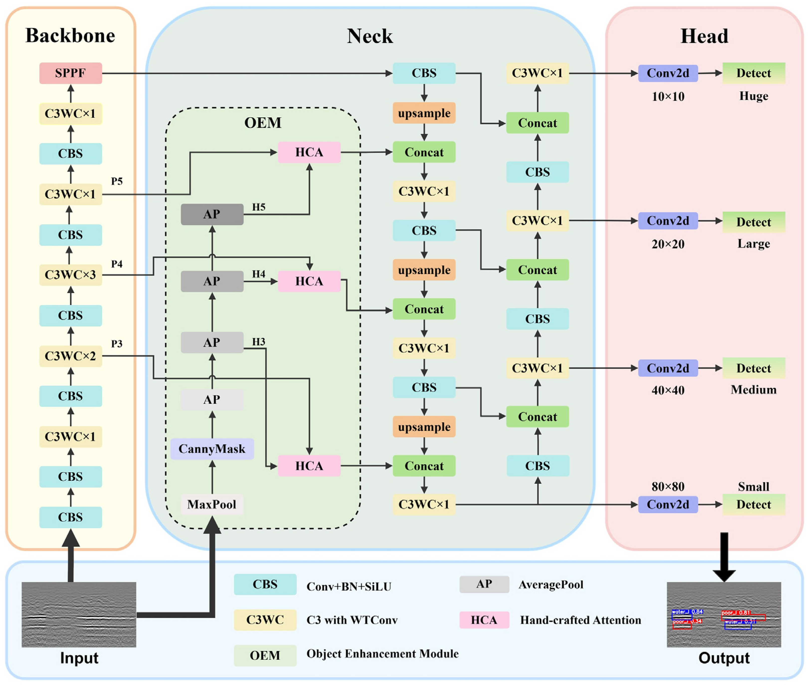
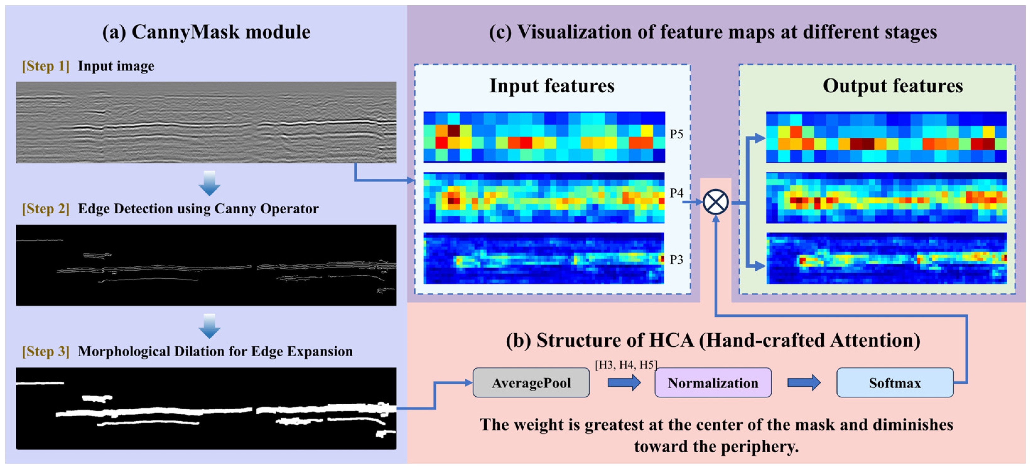
The OEM, based on prior knowledge, is designed and integrated into the YOLOv5s model, which fully leverages edge position information to improve localization and feature representation abilities of the model. This module not only improves the performance of the model but also increases its interpretability of the model;
(3)
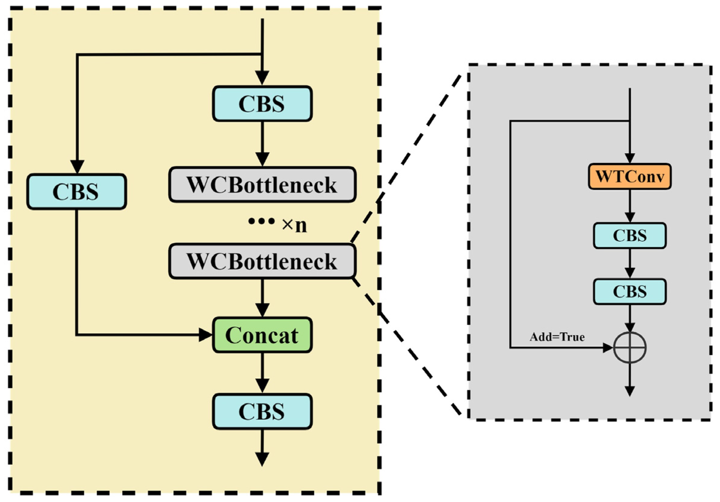
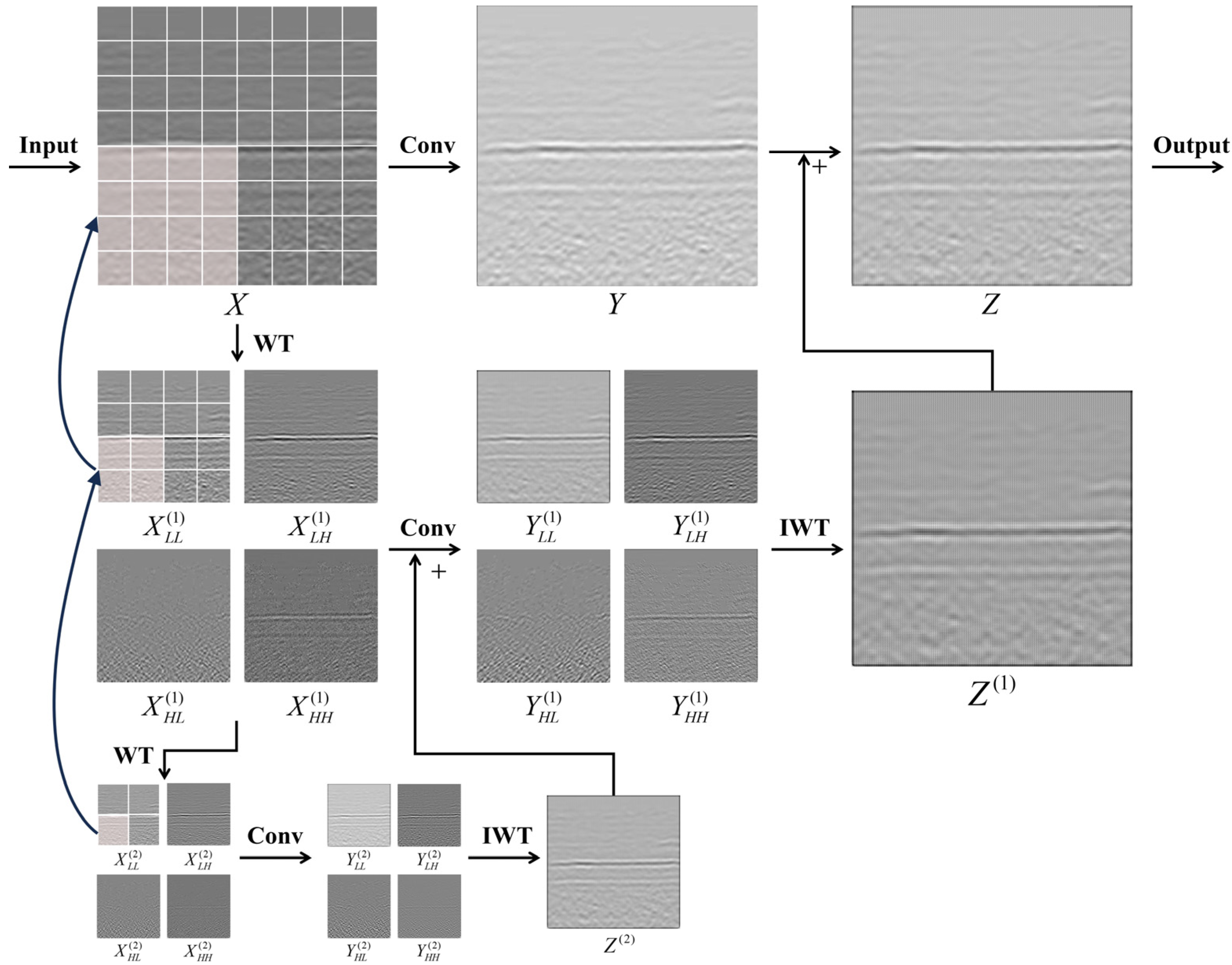
WTConv is introduced into the YOLOv5s model. This approach effectively mitigates the limitations of a convolutional neural network (CNN) in global feature extraction and enhances the model’s ability to capture low-frequency features;
(4)
The number of detection heads for YOLOv5s was extended from three (small, medium, and large) to four (small, medium, large, and huge), which effectively addresses the issue of big variations in sizes of the interlayer distresses and enhances the detection ability of large objects.
The remainder of this paper is described as follows. Section 2 introduces the proposed OEM-HWNet model and the details of module design. Section 3 describes dataset construction and the experimental details. Section 4 analyzes the experimental results. Section 5 summarizes the conclusions of the study.

2. Methodology

To clearly describe the detection model developed in this paper, this section firstly introduces the OEM-HWNet model and its main components. Then, the design of the OEM modules based on prior knowledge is described in detail. Finally, the C3WC module (WTConv embedded in the C3 module) is elaborated.

2.1. Overview of the OEM-HWNet Architecture

YOLOv5 is selected as our baseline model since it has fewer model parameters compared with the latest YOLOv11 [54] and high accuracy. As shown in Figure 3, OEM-HWNet is primarily divided into three parts: the backbone, neck, and head parts.
First, the backbone part comprises the CBS module, C3WC module, and Spatial Pyramid Pooling Fast (SPPF) module. The CBS module includes a standard convolutional layer (Conv2d), a batch normalization (BN) layer, and the SiLU activation function. The original C3 module (three convolutional layers and several Bottleneck modules) is replaced by the C3WC module, integrating the WTConv into the Bottleneck to obtain a larger receptive field and improve the ability to capture low-frequency features. The SPPF module is an optimized version of spatial pyramid pooling (SPP) [55]. Second, the neck part combines Feature Pyramid Networks (FPN) [56] and Path Aggregation Network (PANet) [57], which realize the fusion of semantic information from low level to high level. Notably, a specially designed module called OEM is inserted between the neck and the backbone part. This module focuses on learning of the interlayer distresses and inhibits interference, which significantly improves the learning ability and robustness of the model. Finally, the original YOLOv5s model includes three detection heads with sizes of 20 × 20, 40 × 40, and 80 × 80, respectively. However, these detection heads cannot fully meet the needs of distress detection in the case of interlayer distress with huge scale changes in size. To correct this, we added an additional detection head with a size of 10 × 10 to improve the model’s ability to detect large objects.
Loss function of the OEM-HWNet model consists of classification loss ( L o s s c l s ), object confidence loss ( L o s s o b j ), and box localization loss ( L o s s b o x ), which are expressed as follows:
L o s s = L o s s b o x + L o s s o b j + L o s s c l s
The L o s s b o x denotes the deviation between the truth box and predicted box. Here, the complete-IoU (CIoU) loss [58] is adopted in the localization of the bounding box, which is an improved object detection loss function. So, the L o s s b o x is expressed as follows:
L o s s b o x = L o s s C I O U = 1 I O U + ρ 2 ( b , b g t ) c 2 + α υ
I O U = B B g t B B g t
where B and B g t denote the predicted and ground-truth box, respectively; b and b g t denote the central points of B and B g t , ρ is the Euclidean distance; and c is the diagonal length of the smallest enclosing box covering the two boxes. The α is a positive trade-off parameter and υ measures the consistency of the aspect ratio, as follow:
α = υ ( 1 I O U ) + υ
υ = 4 π 2 ( a r c t a n w g t h g t a r c t a n w h ) 2
where w and w g t represent the widths of predicted box and ground-truth box, respectively, while h and h g t correspond to their heights. Binary cross-entropy loss [41] is employed to calculate the object confidence ( L o s s o b j ) and classification loss ( L o s s c l s ). The former considers both positive and negative samples, while the latter only uses positive ones. The L o s s o b j and L o s s c l s can be expressed as follows:
L o s s o b j = λ o b j i = 0 N 2 j = 0 M I i j o b j [ C ^ i l n C i ( 1 C ^ i ) l n ( 1 C i ) ] + λ n o b j i = 0 N 2 j = 0 M I i j n o b j [ C ^ i l n C i ( 1 C ^ i ) l n ( 1 C i ) ]
L o s s c l s = i = 0 N 2 j = 0 M c c l s I i j o b j [ p ^ i ( c ) l n ( p i ( c ) ) ( 1 p ^ i ( c ) ) l n ( 1 p i ( c ) ) ]
where N 2 stands for the number of grid cells; M represents the number of predicted bounding boxes per grid cell; λ o b j and λ n o b j represent the weights of the grid cell with or without the objects, respectively; I i j o b j and I i j n o b j denote whether there is an object to be predicted in the j-th anchor box of the i-th grid cell, respectively; C ^ i and C i are the confidence of the predicted and truth values, respectively; and p ^ i ( c ) , p i ( c ) are the predicted and truth probabilities of detecting an object belonging to interlayer distress type c in the i-th grid cell, respectively.

2.2. Prior Knowledge

2.2.1. Physical Basis

Figure 4a presents a schematic diagram of the GPR operation, where the antenna pair transmits an electromagnetic wave and receives the echo from the medium. In fact, the GPR obeying the wave equation [59] as
2 E + μ σ 𝜕 E 𝜕 t + μ ε 𝜕 2 E 𝜕 t 2 = 0
where E is electric field strength vector, μ is magnetic permeability, σ is conductivity, ε is permittivity, and t is time.
Strong reflections occur when the electromagnetic wave propagates to the interlayer distresses (Figure 4b). In general, the reflection intensity is determined by the difference in the permittivity of the two mediums, namely
R = ε 2 ε 1 ε 2 + ε 1
where ε 1 and ε 2 are the permittivity of mediums in two adjacent layers. The greater the difference in permittivity, the stronger the reflection. When interlayer distress occurs, the permittivity of the distress is obviously different from that of the surrounding medium, so there is a strong reflected signal, as GPR B-scan images shown in Figure 4c. This principle is critical for non-destructive testing of interlayer distresses in asphalt pavement [60]. For example, interlayer debonding typically manifests as air filling between pavement layers, and the permittivity of air is 1, which is significantly different from the surrounding medium. This will result in a strong reflection, which is manifested in GPR images as the evidence for interlayer distress detection. In addition, higher-frequency antennas provide higher vertical resolution but limited penetration depth, whereas lower frequencies achieve deeper penetration at the cost of reduced resolution [59]. High-frequency antennas are essential to identify subtle changes in permittivity, while lower frequencies may fail to detect early-stage debonding. For the detection of interlayer distresses, the antenna frequency of GPR is typically set within the range of 700 MHz to 1000 MHz.

2.2.2. Object Region Segmentation

The shape and texture features are of importance to identify interlayer distresses in asphalt pavement, so these features extracted from GPR images as prior knowledge are used to segment interlayer distresses from the background. The Canny edge detection algorithm [61] utilizes dual thresholds (high and low thresholds) for object edge extraction and if any part of a contour is above the high threshold, those points are immediately output, as is the entire connected segment of contour, which contains the points and which lies above the low threshold. It has been proved to be effective in extracting the object edges [28]; however, these edges are one continuous line and cannot represent the object region. To separate the object region from the background, morphological dilation [62] is introduced as a complement to the Canny operator to connect neighboring lines to form the object region.
Specifically, the close distance between the upper and lower edges of the object region provides a clue for separating the object area from the background. The CannyMask module first uses the Canny operator to generate texture information and then uses morphological dilation to fill the gap between edges as
CannyMask = Dilation ( 5 , 1 ) ( Canny ( 90 , 225 ) ( X ) )
where Dilation ( 5 , 1 ) denotes the dilation operation with a kernel size of 5 × 5 and iterations of 1 to fill the gap, Canny ( 90 , 225 ) represents the Canny operator with a low threshold of 90 and a high threshold of 225, X is the input image, and CannyMask is the mask tensor representing object area. For the mask tensor, the pixel value of the object region is set to 255, and the background region is set to 0.
As shown in Figure 5, CannyMask can separate the object region from the background, but there are still limitations. First of all, the edge detection method based on prior knowledge cannot adapt to various complex backgrounds, which refer to non-target signals including measurement noise, normal pavement structure, and other distresses. For example, the crack shown in the yellow circle of sample 2 in Figure 5 belongs to other distresses, but this area with continuous strong gray-scale variations and hyperbolic characteristics may be prone to be confused with interlayer distresses. The regions identified by CannyMask encompass the interlayer distresses and other types of distresses, such as cracks. However, not only can CannyMask suppress most of the background interference but it also enhances the region features identified by CannyMask, which significantly contributes to improving the recognition performance of deep learning-based networks. In addition, although CannyMask can locate the object region well, it cannot further classify the object region as interlayer debonding or interlayer water seepage. It is worth noting that deep learning-based networks can solve the above classification problems, but inaccurate localization often occurs in object detection. Therefore, as an a priori feature module, CannyMask may be embedded into the deep learning network to improve the location ability of detection network.

2.3. Object Enhancement Module (OEM) Based on Prior Knowledge

An OEM based on the prior knowledge is designed as shown in Figure 3. The OEM has two inputs: the original image and the input features (the output of the previous module). Firstly, the object area of the original image is extracted through the MaxPool and subsequent CannyMask module (Figure 6a). Secondly, in order to ensure the same scale of input features, the CannyMask module is followed by the AP (AveragePool) module. Thirdly, the output of the AveragePool module is normalized, and the weight matrix is generated by the softmax function shown in Figure 6b. Finally, the output features are obtained by multiplying the weight matrix with the input features shown in Figure 6c. This module not only enhances the object region but also adds no additional parameters. The mathematical expression of this process is as follows:
H n = AP n 1 ( CM [ MP ( X ) ] )
Ouput = P n × S o f t m a x ( N o r m a l i z a t i o n ( H n ) )
where H n represents the hand-crafted features based on the Canny operator and morphological dilation for all stages and X is the original image. AP ( ) , CM ( ) , and MP ( ) perform AveragePool, CannyMask, and MaxPool, respectively. In Formula (12), P n represents the input features for all stages and n is the stage number.
The OEM provides a new solution to some problems of the detection model, such as poor object positioning and unfocused learning. By incorporating prior knowledge, the model performance is significantly enhanced. A key advantage of this module is its parameter-free nature. Furthermore, the OEM helps to quickly locate the object region so that the learning of the model can be focused on that region, thus accelerating convergence.

2.4. C3WC Module

The size of the convolution kernel limits the global modeling capabilities of CNN. So, many researchers have attempted to increase the kernel size of CNN to mimic the global receptive field found in self-attention mechanisms. However, this method quickly hit an upper bound and saturated way before achieving a global receptive field. To address this challenge, Finder et al. proposed the WTConv based on wavelet transform, which excels at extracting features with different scales [51]. In this paper, the WTConv is integrated into the C3 module, named C3WC (Figure 7), to obtain a larger receptive field. As shown in the grid of Figure 8, a 1 × 1 convolution, which is performed on the low-frequency band of the second-level wavelet domain X L L ( 2 ) , is a response to lower frequencies of a 4 × 4 receptive field in the input X . The process is given by
Y = I W T ( C o n v ( W , W T ( X ) ) )
where X is the input tensor, and W is the weight tensor of a k × k depth-wise kernel with four times as many input channels as X . In this study, we employ 5 × 5 kernel sizes for the convolutions.
Figure 8 illustrates the WTConv process with a 2-level wavelet transform. The initial step performs decomposition of the input signal into multi-scale wavelets. Subsequently, different frequency bands are processed using depth-wise convolution [63] with small convolution kernels, followed by image reconstruction through an inverse wavelet transform (IWT) to obtain the final output. The decomposition is given by
( X L L ( i ) ,   X H L ( i ) ,   X L H ( i ) ,   X H H ( i ) ) = WT ( X L L ( i 1 ) )
where X L L ( 0 ) = X and i is the current level. X L L ( i ) is the low-frequency component of X , while X L H ( i ) , X H L ( i ) , and X H H ( i ) are its horizontal, vertical, and diagonal high-frequency components. The Formulas (15) and (16) describe convolution and inverse wavelet transform (IWT), respectively.
( Y L L ( i ) ,   Y H L ( i ) ,   Y L H ( i ) ,   Y H H ( i ) ) = Conv ( W ( i ) ,   ( X L L ( i ) ,   X H L ( i ) ,   X L H ( i ) ,   X H H ( i ) ) )
Z ( i ) = IWT ( Y L L ( i ) + Z ( i + 1 ) , Y H L ( i ) ,   Y L H ( i ) ,   Y H H ( i ) )
where Z ( i ) is the aggregated outputs from level i onward. As observed in Figure 8, WTConv performs repetitive wavelet decomposition on the low-frequency band of the input image, continuously enhancing low-frequency features. WTConv has a superior capacity for capturing low-frequency information compared to standard convolution. Moreover, each level of WTConv increases the receptive field size while only marginally increasing the number of trainable parameters. This characteristic is a significant factor in integrating WTConv into the C3 module. In this study, we employ a 3-level wavelet decomposition to make a trade-off between accuracy and the number of parameters.

3. Validation Using Field Tests

3.1. Dataset

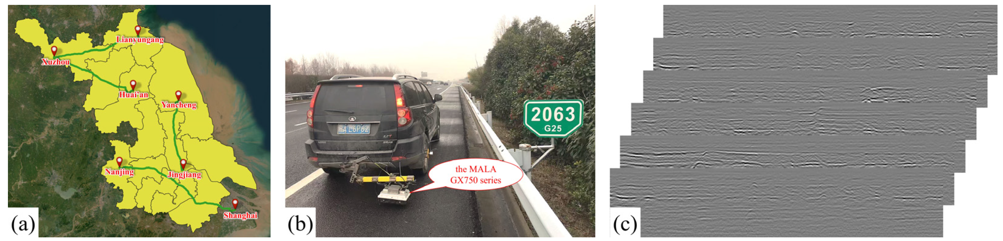
3.1.1. Data Acquisition

In interlayer distress detection of asphalt pavement within GPR images, no public dataset currently exists. To evaluate the performance of the proposed model, this study collected thousands of GPR images from several highways, including the Lianyungang-Xuzhou Highway, Huai’an-Xuzhou Highway, Yancheng–Jingjiang Highway, and Shanghai-Nanjing Highway, in Jiangsu province of China, as shown in Figure 9a.
Field data collection was conducted using the fourth-generation high-dynamic GPR, the MALA GX750 series (Figure 9b), produced by the Swedish company GuidelineGEO in Stockholm, Sweden. Its technical specifications are as follows: antenna frequency of 750 MHz, scanning speed of 1290 (traces/s), detection depth ranging from 0 to 1.5 m, air-coupling antenna mode, weight of 3.6 kg, and detection vehicle speed of 80 (km/h). After pre-processing, such as dewow, adjustment of start time, compensation for energy decay, background removal, deconvolution, and bandpass filtering, we obtained a total of 2105 GPR images (Figure 9c). Each image is with a width of 1005 pixels and a height of 210 pixels, corresponding to the length of 20 m and the time window of 20 ns, respectively.

3.1.2. Dataset Construction

Through the analysis of the above GPR images, we find that the main hidden distresses of asphalt pavement are interlayer distresses, so interlayer distresses become the research object of this paper. Further analysis of interlayer distresses shows that although the shape characteristics of interlayer distresses at different positions are similar, there are differences in vertical texture characteristics, as shown in Figure 10. By comparing and analyzing the image and the corresponding drilled sample core, combined with the experience of experts in the field, the interlayer distresses can be classified as interlayer debonding (Figure 10a) and interlayer water seepage (Figure 10b). This accurate classification of interlayer distresses is of importance to improve maintenance efficiency and reduce maintenance costs. For interlayer debonding, the pressure grouting is adopted to fill the gap between the layers of pavement [64], while interlayer water seepage is a more serious issue, requiring both pressure grouting and drainage system repair.
Figure 10 shows the GPR images and core samples of two categories of interlayer distress. In Figure 10, the red square represents the location of the distress, “a” indicates the interface of the surface layer and the upper base layer, “b” denotes the interface of the upper base layer and the lower base layer, “c” indicates the interface of the lower base layer and the subbase layer, and “d” denotes the coring position.
The characteristics of interlayer debonding and interlayer water seepage are described as follows:
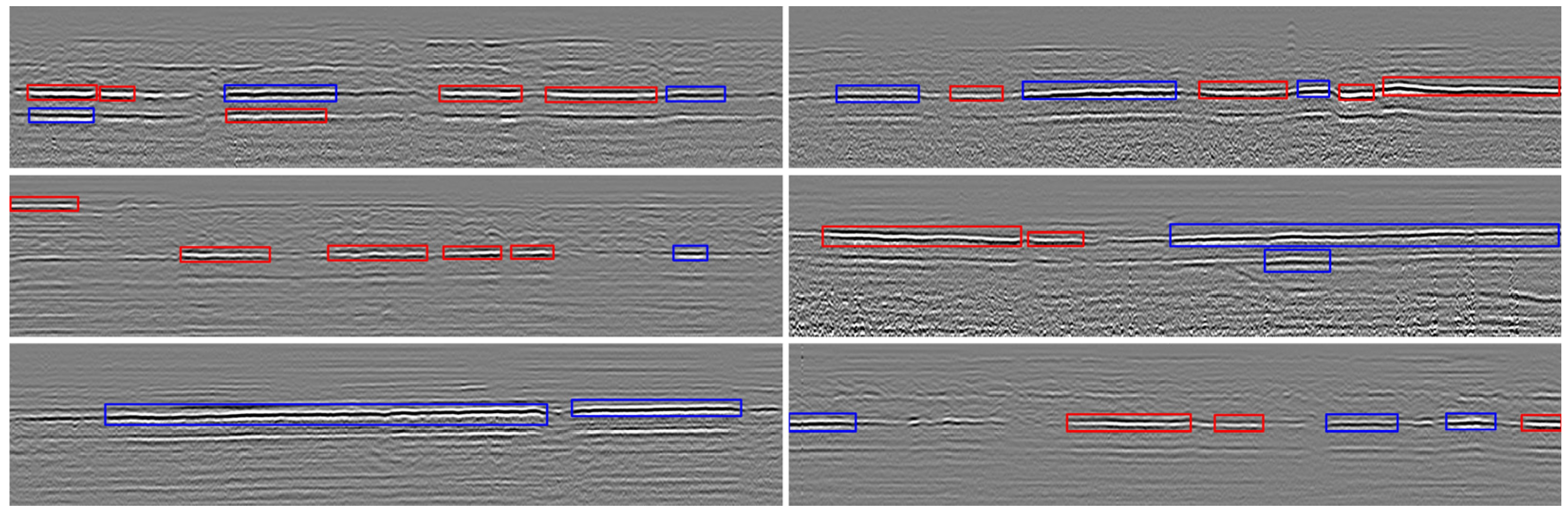
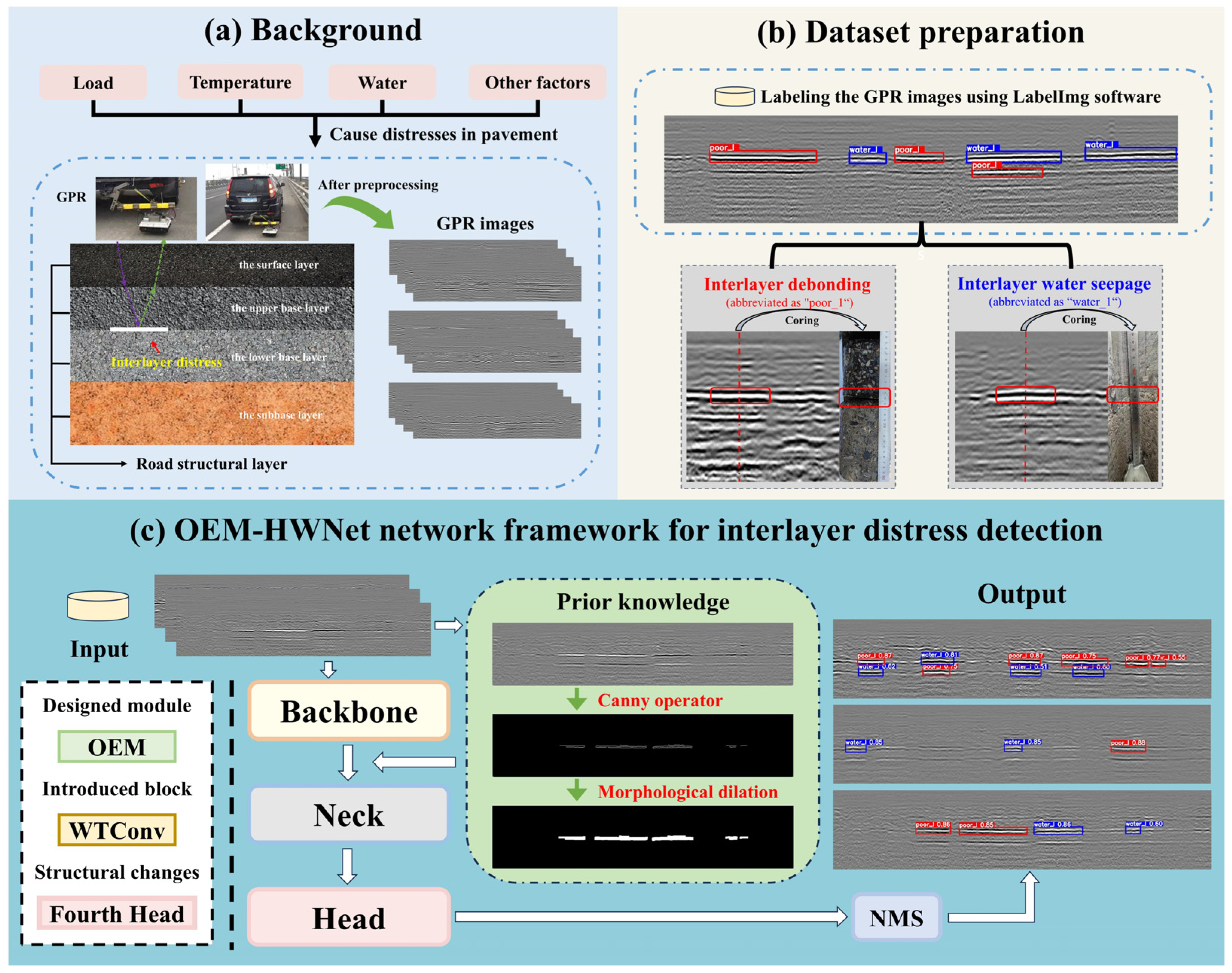
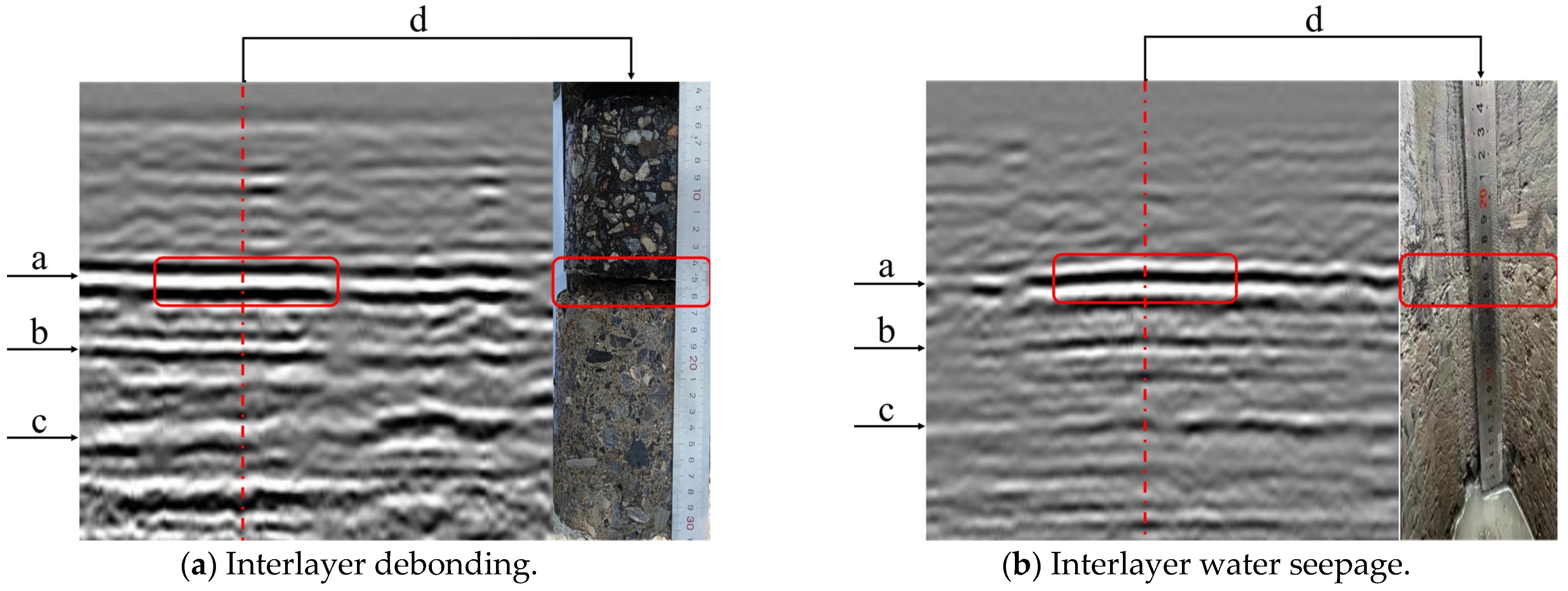
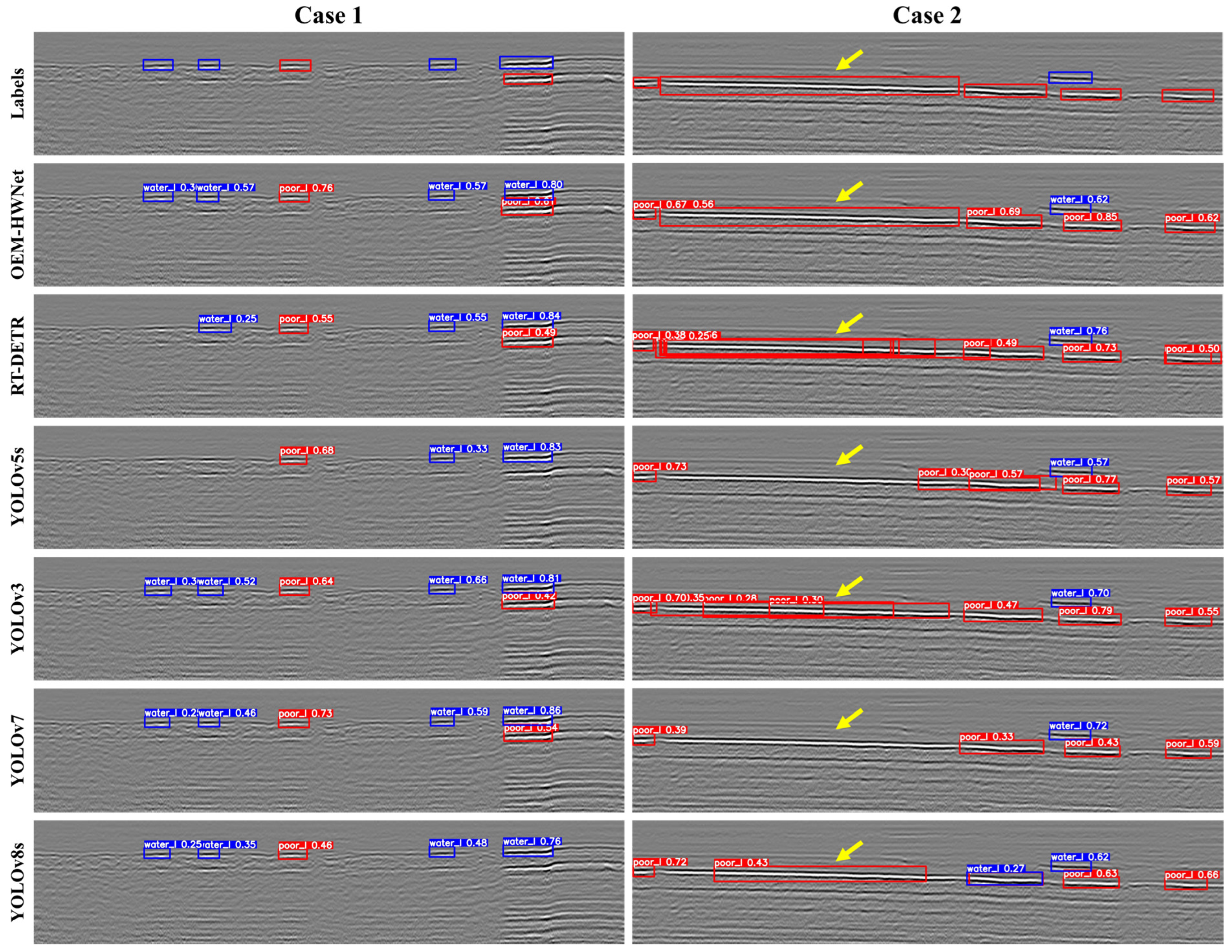
  • Interlayer debonding: temperature, load, or other factors may cause a continuous separation between the layers of pavement, and interlayer delamination occurs, named interlayer debonding. There is a strong reflection in the GPR image due to the difference in permittivity of the air contained between the layers and the surrounding medium. Specifically, the image features of interlayer debonding appear as black, white, and black in vertical order (Figure 10a). Interlayer debonding is abbreviated as “poor_1”;
  • Interlayer water seepage: when interlayer debonding has occurred without timely maintenance, interlayer water seepage distress between the layers occurs as rainwater seeps in. Unlike other air-containing distresses, this category of distress contains water. The permittivity of water and air are different, typically 81 for water and 1 for air. As a result, Figure 10b shows a clear polarity reversal for interlayer water seepage compared to interlayer debonding. Specifically, the image features of interlayer water seepage appear as white, black, and white in vertical order. Interlayer water seepage is abbreviated as “water_1”.
We used LabelImg 1.8.6 software to annotate the 2105 GPR images. An annotated example is shown in Figure 11, where the red box indicates interlayer debonding and blue indicates interlayer water seepage. Table 1 summarizes the basic situation of the interlayer distresses, including the total number of samples and scale statistics of interlayer debonding, as well as interlayer water seepage. The average size indicates that the bounding boxes for interlayer debonding and interlayer water seepage are similar in size. In the field of object detection, the annotated areas less than 10% of an image belong to small objects [65]. However, the average area of interlayer distresses accounted for only 8% of the GPR images, which poses a challenge for the identification of interlayer debonding and interlayer water seepage. The maximum and minimum width values reveal that the size variability of the interlayer distresses predominantly occurs in width, with a difference of approximately 25 times. The big variation in size further increases the difficulty of detection. For all experiments conducted in this study, the dataset was partitioned into training, validation, and test sets in a ratio of 8:1:1.

3.2. Evaluation Metrics and Experimental Configuration

To accurately and fairly evaluate the performance of the OEM-HWNet, we employed several metrics, including precision ( P ), recall ( R ), and F 1 score. The computations of these indicators are presented below, as follows:
P = T P T P + F P
R = T P T P + F N
F 1 = 2 P R P + R
where T P is the true positive, F P is the false positive, F N is the false negative, and T N is the true negative. Mean average precision ( m A P ) is typically employed for the evaluation of multi-distress detection systems. In this context, it represents the average precision for interlayer distress detection. The precision–recall ( P R ) curve is illustrated with recall on the horizontal axis and precision on the vertical axis. Average Precision (AP) denotes the area under the P R curve, calculated at various thresholds for a specific distress category. The metrics m A P @ 0.5 can be expressed as follows:
m A P @ 0.5 = i = 0 n 0 1 P R d R I O U t h r e s h = 0.5
In this study, the proposed interlayer distress detection model of asphalt pavement was performed on a server with an Intel(R) Xeon(R) Gold 6133 CPU and a single NVIDIA GeForce RTX 3090 GPU. The software environment configuration of the model is shown in Table 2. The batch size and epoch for all experiments were set to 16 and 200, respectively. The initial learning rate was 0.01, and the learning rate decay followed a cosine schedule. The SGD [66] algorithm was selected as the optimizer with the momentum of 0.937 and decay weight of 0.0005.

4. Experimental Results

4.1. Preliminary Analysis of OEM-HWNet

4.1.1. Detection Results of OEM-HWNet

Confusion matrix is a common form of presenting and analyzing test results. The training and testing were carried out on the established GPR dataset, and the test results obtained were shown in Figure 12. The values in each cell represent the ratio of the predicted number and the true number of samples for each category. The “background” in the horizontal axis represents the situation in which the background is misjudged as the distress, whereas the “background” in the vertical axis represents the situation in which the distress is misjudged as the background. The analysis of Figure 12 is as follows. First, the main diagonal of the confusion matrix indicates that the OEM-HWNet model can identify the interlayer distresses with high accuracy, in which the scores of interlayer debonding and interlayer water seepage are 0.89 and 0.94, respectively. Then, the scores of interlayer debonding and interlayer water seepage from the “background” in the vertical axis are 0.08 and 0.05, respectively; it means that a small number of distresses are not recognized. In addition, the scores of interlayer debonding and interlayer water seepage from the “background” in the horizontal axis not only show that the interlayer distress and other distress in the background have similar characteristics but also the characteristics of interlayer debonding and interlayer water seepage are also very similar. Although interlayer disease detection is a difficult task, the OEM-HWNet still demonstrates excellent performance. To further demonstrate the detection performance of the proposed network, Figure 13 shows a comparison between the detection results and the ground-truth labels. From Figure 13, we can see that the detection results are almost consistent with the ground-truth label. This indicates that the OEM-HWNet performed well in accurately locating and identifying interlayer distresses.

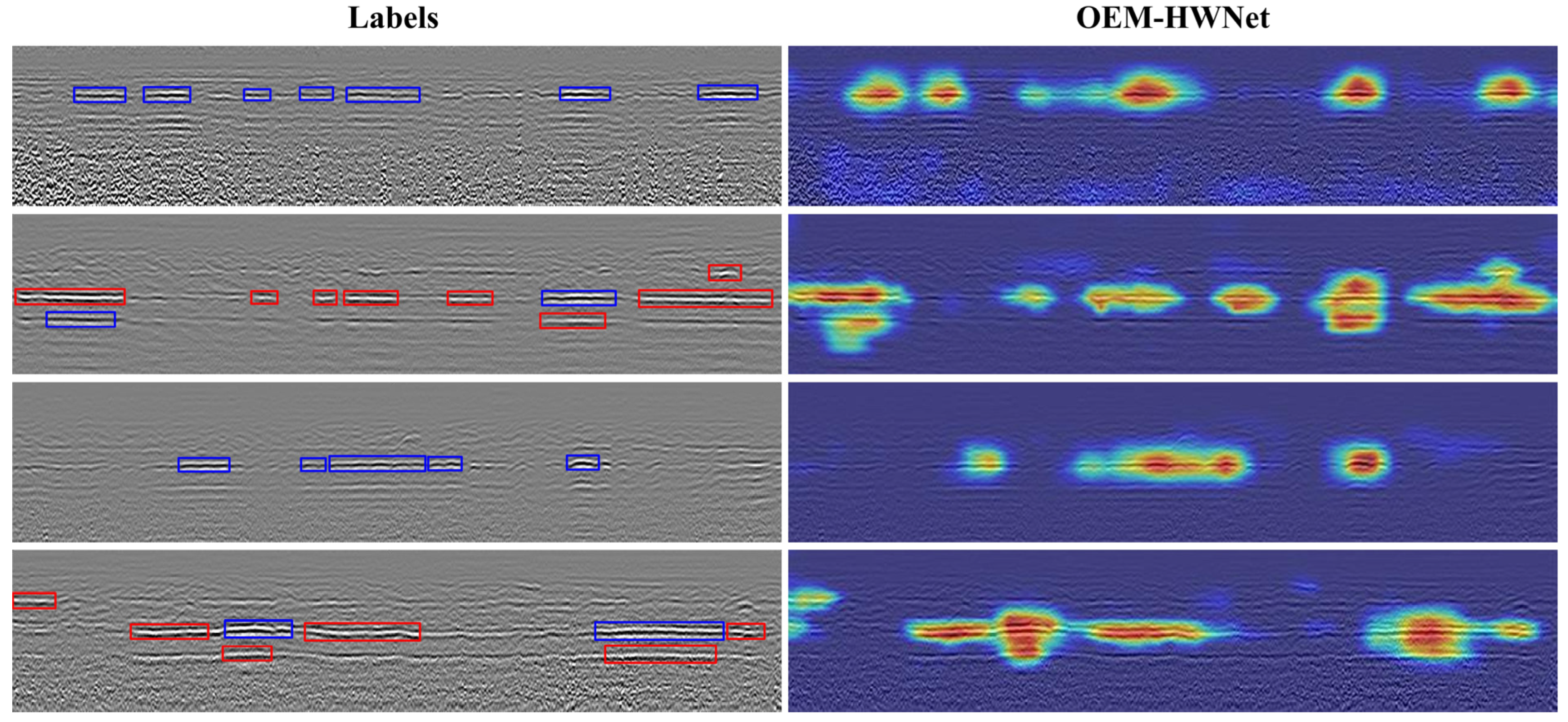
4.1.2. Visualization of Attention Maps

To clearly understand the decision-making process of the OEM-HWNet network in recognizing interlayer distress, Grad-CAM [67] is employed to visualize the attention maps within the network architecture. Figure 14 presents the visualized attention maps from the output of the final layer. Notably, red indicates the areas that the network focuses on during the decision-making process. In contrast, blue indicates the less important areas. It can be observed that the red areas and the ground-truth labels are almost identical in position. This indicates that the prior knowledge-guided network can accurately locate and focus learning on interlayer distress. Although there are a few red or yellow areas appearing in the background, a clear distinction can be seen between interlayer distress and the background.

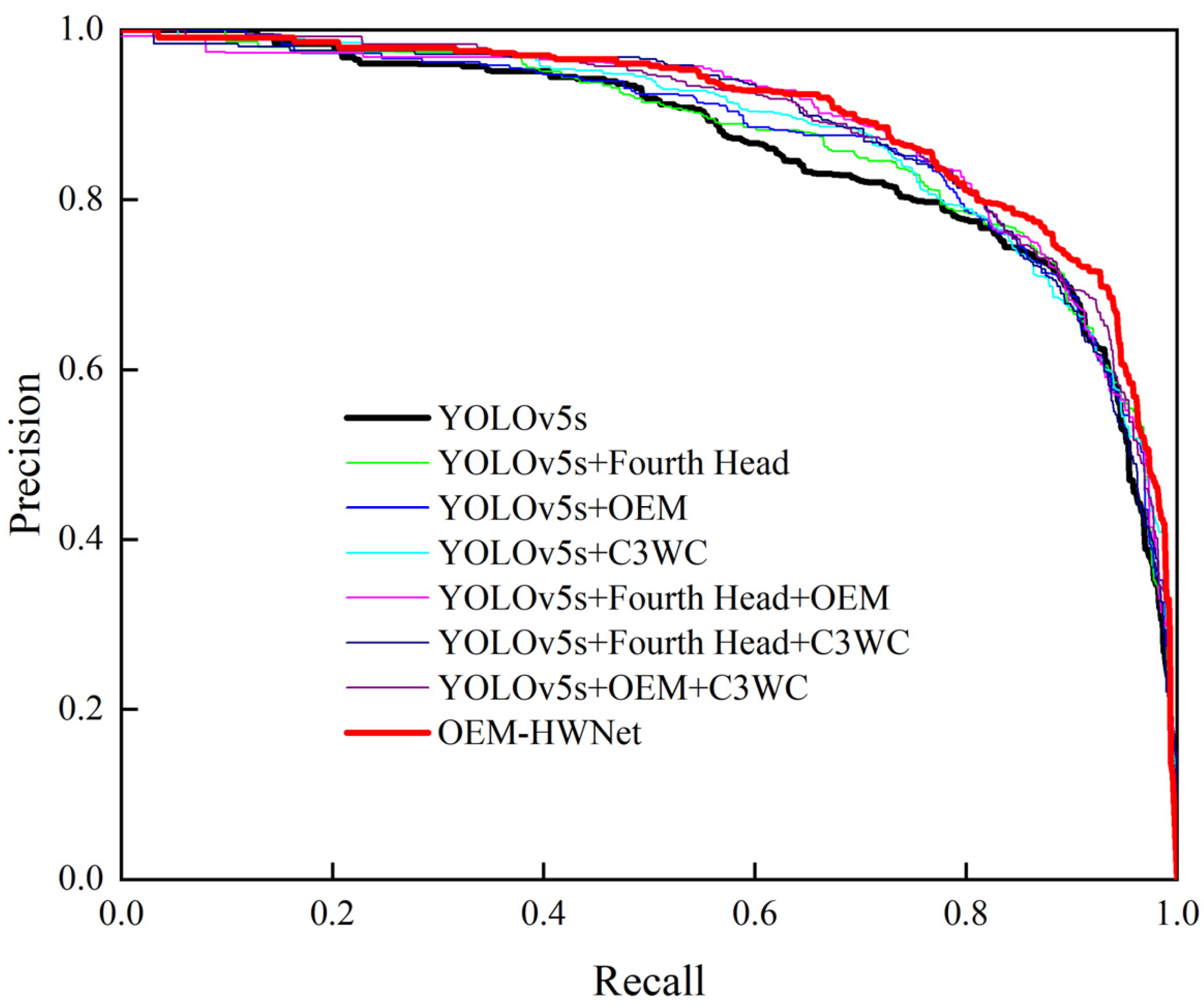
4.2. Ablation Experiments

Relative to the YOLOv5s model, the improved parts of the OEM-HWNet model include the OEM, the fourth head, and the C3WC module. To demonstrate the effectiveness of each module and combination of modules, ablation experiments were performed. The evaluation indices used in ablation experiments include average precision (AP), mean average precision (mAP) at a threshold of 0.5, parameter count (parameters), precision (P), recall (R), and F1.
The experimental results are presented in Table 3. The analysis of Table 3 is described as follows. Firstly, adding a detection head (Fourth Head), introducing the OEM module, and incorporating the C3WC module obtains the improvements of 0.7%, 1.0%, and 1.5% in mAP, respectively. Secondly, the combination of the OEM and Fourth Head resulted in a 2.2% increase in mAP, while the joint use of the OEM and C3WC brought a mAP improvement of 2.5%. More importantly, the introduction of the OEM module does not add additional training load because of its parameter-free nature. Finally, the coupling of the three blocks resulted in a 3.3% increase in mAP. The experimental results verify that the proposed OEM-HWNet is a very competitive solution for the accurate detection of interlayer distresses.
The P R curves provide an intuitive representation of model performance. Figure 15 compares the P R curves of the different models within the dataset of this study. The larger the area under the P R curve, the better the performance of the model. Compared with YOLOv5s, the area under the P R curve of all recommended improved models has been increased, among which the OEM-HWNet model has the largest area.

4.3. Comparison with the State-of-the-Art Methods

In order to verify the effectiveness of the proposed OEM-HWNet model, the current state-of-the-art object detection models, such as Faster R-CNN, RetinaNet, SSD, RT-DETR, YOLOv3, YOLOv5, YOLOv7, YOLOv8, and YOLOv11, are chosen to compare with our model. To ensure a fair comparison, a consistent operating environment and datasets are used.
Table 4 presents a quantitative comparison in Average Precision (AP), mean average precision (mAP), model size, and Frames Per Second (FPS) for the aforementioned models evaluated on the same test set. Firstly, the Faster R-CNN, RT-DETR, and YOLO series are similar in mAP, but YOLOv5s has the smallest size and the fastest detection speed. Therefore, we chose YOLOv5 as the baseline model. Secondly, compared with YOLOv5s, although the incorporation of the Fourth Head and C3WC modules increases the number of model parameters and leads to a decrease from 160 to 84 in FPS, the proposed OEM-HWNet model can still meet the requirement of real-time detection of interlayer distresses. Finally, the proposed OEM-HWNet model presents the highest AP and mAP for both categories of interlayer distresses, although YOLOv5s, YOLOv8s, and YOLOv11s have smaller model size and faster inference speed. In addition, for all models, the detection accuracy of interlayer water seepage is higher than that of interlayer debonding because the GPR image of interlayer water seepage has polarity reversal in the vertical direction, which makes its features more discriminative.
The qualitative assessment is crucial in understanding how these methods perform in real-time detection. Among the state-of-the-art methods, RT-DETR, YOLOv3, YOLOv5s, YOLOv7, and YOLOv8s have a higher mAP; therefore, these methods are selected to analyze furtherly. Figure 16 shows some detection results of the above methods and OEM-HWNet. As the position indicated by the yellow arrow in case 2 in Figure 16, the OEM-HWNet can detect the large-scale interlayer distress with accurate location and high confidence but YOLOv5s and YOLOv7 can not. Although RT-DETR, YOLOv3, and YOLOv8s may detect the large-scale interlayer distress, they may not detect it accurately. The results indicate that the network requires a larger receptive field for detecting large-scale distress accurately. Moreover, as shown in case 1 of Figure 16, some distresses have not been detected in the detection results of YOLOv5s, while OEM-HWNet can detect all interlayer distresses. The comparison results indicate that OEM, based on prior knowledge, can help detect model precision positioning and focused learning. In summary, OEM-HWNet, including Fourth Head, OEM, and C3WC modules, demonstrates excellent performance in interlayer distress detection.

5. Conclusions

In this study, a prior knowledge-guided network called OEM-HWNet was designed to detect the interlayer distress of asphalt pavement with GPR images. Specifically, the OEM, based on prior knowledge, significantly improves network performance without imposing additional parameters. The C3WC module was introduced to obtain a larger receptive field and enhance the low-frequency information. An additional detection head was added to enhance the detection capability of large objects. The conclusions are drawn as follows:
(1)
The existing methods may cause inaccurate locations for interlayer distress due to the interference of similar background features. Based on prior knowledge, the OEM can accurately locate the object region to allow the focusing of the learning of the model on that region without imposing additional parameters;
(2)
The proposed OEM-HWNet model achieves an average precision (AP) of 87.8% for interlayer debonding and 91.5% for interlayer water seepage, resulting in a mAP of 89.6%. Meanwhile, the comparative results with the original YOLOv5s model represent a 3.3% increase in mAP. Moreover, the results also indicate that the OEM-HWNet model surpasses other advanced models in detection accuracy;
(3)
The proposed method may be used for automatic and real-time interlayer distress detection of asphalt pavement using GPR. An extensive GPR dataset from four highways was constructed to evaluate the detection model rigorously. Future research may validate the proposed method with more testing datasets from asphalt pavement. Incorporating more interpretable prior knowledge to guide the design of the detection network is suggested.

Author Contributions

Conceptualization, C.L.; methodology, C.L. and S.C.; software, S.C.; validation, S.C. and X.W.; formal analysis, C.L.; investigation, C.L.; resources, C.L.; data curation, G.J.; writing—original draft preparation, C.L. and S.C.; writing—review and editing, C.L., S.C. and S.W.; visualization, W.C.; supervision, C.L.; project administration, C.L.; funding acquisition, C.L. All authors have read and agreed to the published version of the manuscript.

Funding

This research was funded by the National Key Research and Development Program of China (2022YFC3003202).

Data Availability Statement

Data will be made available on request.

Conflicts of Interest

Authors Guanglai Jin and Wenlong Cai were employed by the company Jiangsu Sinoroad Engineering Technology Research Institute Co., Ltd. The remaining authors declare that the research was conducted in the absence of any commercial or financial relationships that could be construed as a potential conflict of interest.

References

  1. Solla, M.; Pérez-Gracia, V.; Fontul, S. A Review of GPR Application on Transport Infrastructures: Troubleshooting and Best Practices. Remote Sens. 2021, 13, 672. [Google Scholar] [CrossRef]
  2. Wang, S.; Zhao, S.; Al-Qadi, I.L. Real-Time Density and Thickness Estimation of Thin Asphalt Pavement Overlay During Compaction Using Ground Penetrating Radar Data. Surv. Geophys. 2020, 41, 431–445. [Google Scholar] [CrossRef]
  3. Xu, X.; Peng, S.; Xia, Y.; Ji, W. The Development of a Multi-Channel GPR System for Roadbed Damage Detection. Microelectron. J. 2014, 45, 1542–1555. [Google Scholar] [CrossRef]
  4. Todkar, S.S.; Le Bastard, C.; Baltazart, V.; Ihamouten, A.; Derobort, X. Comparative Study of Classification Algorithms to Detect Interlayer Debondings within Pavement Structures from Step-Frequency Radar Data. In Proceedings of the IGARSS 2018—2018 IEEE International Geoscience and Remote Sensing Symposium, Valencia, Spain, 22–27 July 2018; IEEE: New York, NY, USA, 2018; pp. 6820–6823. [Google Scholar]
  5. Guo, S.; Xu, Z.; Li, X.; Zhu, P. Detection and Characterization of Cracks in Highway Pavement with the Amplitude Variation of GPR Diffracted Waves: Insights from Forward Modeling and Field Data. Remote Sens. 2022, 14, 976. [Google Scholar] [CrossRef]
  6. Xu, J.; Zhang, J.; Sun, W. Recognition of the Typical Distress in Concrete Pavement Based on GPR and 1D-CNN. Remote Sens. 2021, 13, 2375. [Google Scholar] [CrossRef]
  7. Zhang, J.; Yang, X.; Li, W.; Zhang, S.; Jia, Y. Automatic Detection of Moisture Damages in Asphalt Pavements from GPR Data with Deep CNN and IRS Method. Autom. Constr. 2020, 113, 103119. [Google Scholar] [CrossRef]
  8. Liang, X.; Yu, X.; Chen, C.; Jin, Y.; Huang, J. Automatic Classification of Pavement Distress Using 3D Ground-Penetrating Radar and Deep Convolutional Neural Network. IEEE Trans. Intell. Transp. Syst. 2022, 23, 22269–22277. [Google Scholar] [CrossRef]
  9. Hou, F.; Lei, W.; Li, S.; Xi, J. Deep Learning-Based Subsurface Target Detection From GPR Scans. IEEE Sens. J. 2021, 21, 8161–8171. [Google Scholar] [CrossRef]
  10. Yamaguchi, T.; Mizutani, T.; Meguro, K.; Hirano, T. Detecting Subsurface Voids From GPR Images by 3-D Convolutional Neural Network Using 2-D Finite Difference Time Domain Method. IEEE J. Sel. Top. Appl. Earth Obs. Remote Sens. 2022, 15, 3061–3073. [Google Scholar] [CrossRef]
  11. Li, N.; Wu, R.; Li, H.; Wang, H.; Gui, Z.; Song, D. MV-GPRNet: Multi-View Subsurface Defect Detection Network for Airport Runway Inspection Based on GPR. Remote Sens. 2022, 14, 4472. [Google Scholar] [CrossRef]
  12. Li, H.; Li, N.; Wu, R.; Wang, H.; Gui, Z.; Song, D. GPR-RCNN: An Algorithm of Subsurface Defect Detection for Airport Runway Based on GPR. IEEE Robot. Autom. Lett. 2021, 6, 3001–3008. [Google Scholar] [CrossRef]
  13. Kim, N.; Kim, S.; An, Y.-K.; Lee, J.-J. Triplanar Imaging of 3-D GPR Data for Deep-Learning-Based Underground Object Detection. IEEE J. Sel. Top. Appl. Earth Obs. Remote Sens. 2019, 12, 4446–4456. [Google Scholar] [CrossRef]
  14. Yang, J.; Ruan, K.; Gao, J.; Yang, S.; Zhang, L. Pavement Distress Detection Using Three-Dimension Ground Penetrating Radar and Deep Learning. Appl. Sci. 2022, 12, 5738. [Google Scholar] [CrossRef]
  15. Liu, C.; Du, Y.; Yue, G.; Li, Y.; Wu, D.; Li, F. Advances in Automatic Identification of Road Subsurface Distress Using Ground Penetrating Radar: State of the Art and Future Trends. Autom. Constr. 2024, 158, 105185. [Google Scholar] [CrossRef]
  16. Li, Y.; Liu, C.; Yue, G.; Gao, Q.; Du, Y. Deep Learning-Based Pavement Subsurface Distress Detection via Ground Penetrating Radar Data. Autom. Constr. 2022, 142, 104516. [Google Scholar] [CrossRef]
  17. Li, S.; Gu, X.; Xu, X.; Xu, D.; Zhang, T.; Liu, Z.; Dong, Q. Detection of Concealed Cracks from Ground Penetrating Radar Images Based on Deep Learning Algorithm. Constr. Build. Mater. 2021, 273, 121949. [Google Scholar] [CrossRef]
  18. Liu, Z.; Wu, W.; Gu, X.; Li, S.; Wang, L.; Zhang, T. Application of Combining YOLO Models and 3D GPR Images in Road Detection and Maintenance. Remote Sens. 2021, 13, 1081. [Google Scholar] [CrossRef]
  19. Xiong, X.; Meng, A.; Lu, J.; Tan, Y.; Chen, B.; Tang, J.; Zhang, C.; Xiao, S.; Hu, J. Automatic Detection and Location of Pavement Internal Distresses from Ground Penetrating Radar Images Based on Deep Learning. Constr. Build. Mater. 2024, 411, 134483. [Google Scholar] [CrossRef]
  20. Zhang, J.; Lu, Y.; Yang, Z.; Zhu, X.; Zheng, T.; Liu, X.; Tian, Y.; Li, W. Recognition of Void Defects in Airport Runways Using Ground-Penetrating Radar and Shallow CNN. Autom. Constr. 2022, 138, 104260. [Google Scholar] [CrossRef]
  21. Liu, Q.; Yan, S. Measurement and Assessement of Road Poor Interlayer Bonding Assessment Using Ground Penetrating Radar. In Proceedings of the 2023 5th International Conference on Intelligent Control, Measurement and Signal Processing (ICMSP), Chengdu, China, 19–21 May 2023; pp. 671–674. [Google Scholar] [CrossRef]
  22. Xue, B.; Gao, J.; Hu, S.; Li, Y.; Chen, J.; Pang, R. Ground Penetrating Radar Image Recognition for Earth Dam Disease Based on You Only Look Once V5s Algorithm. Water 2023, 15, 3506. [Google Scholar] [CrossRef]
  23. Liu, C.; Yao, Y.; Li, J.; Qian, J.; Liu, L. Research on Lightweight GPR Road Surface Disease Image Recognition and Data Expansion Algorithm Based on YOLO and GAN. Case Stud. Constr. Mater. 2024, 20, e02779. [Google Scholar] [CrossRef]
  24. Xiong, X.; Tan, Y.; Hu, J.; Hong, X.; Tang, J. Evaluation of Asphalt Pavement Internal Distresses Using Three-Dimensional Ground-Penetrating Radar. Int. J. Pavement Res. Technol. 2024, 1–12. [Google Scholar] [CrossRef]
  25. Jiang, B.; Xu, L.; Cao, Z.; Yang, Y.; Sun, Z.; Xiao, F. Interlayer Distress Characteristics and Evaluations of Semi-Rigid Base Asphalt Pavements: A Review. Constr. Build. Mater. 2024, 431, 136441. [Google Scholar] [CrossRef]
  26. Jin, G.; Liu, Q.; Cai, W.; Li, M.; Lu, C. Performance Evaluation of Convolutional Neural Network Models for Classification of Highway Hidden Distresses with GPR B-Scan Images. Appl. Sci. 2024, 14, 4226. [Google Scholar] [CrossRef]
  27. Cai, W.; Li, M.; Jin, G.; Liu, Q.; Lu, C. Comparison of Residual Network and Other Classical Models for Classification of Interlayer Distresses in Pavement. Appl. Sci. 2024, 14, 6568. [Google Scholar] [CrossRef]
  28. Bugarinović, Ž.; Pajewski, L.; Ristić, A.; Vrtunski, M.; Govedarica, M.; Borisov, M. On the Introduction of Canny Operator in an Advanced Imaging Algorithm for Real-Time Detection of Hyperbolas in Ground-Penetrating Radar Data. Electronics 2020, 9, 541. [Google Scholar] [CrossRef]
  29. Harkat, H.; Dosse Bennani, S. Ground Penetrating Radar Imaging for Buried Cavities in a Dispersive Medium: Profile Reconstruction Using a Modified Hough Transform Approach and a Time-Frequency Analysis. Int. J. Commun. Antenna Propag. IRECAP 2015, 5, 78. [Google Scholar] [CrossRef]
  30. Todkar, S.S.; Le Bastard, C.; Baltazart, V.; Ihamouten, A.; Dérobert, X. Performance Assessment of SVM-Based Classification Techniques for the Detection of Artificial Debondings within Pavement Structures from Stepped-Frequency A-Scan Radar Data. NDT E Int. 2019, 107, 102128. [Google Scholar] [CrossRef]
  31. Frigui, H.; Gader, P. Detection and Discrimination of Land Mines in Ground-Penetrating Radar Based on Edge Histogram Descriptors and a Possibilistic K-Nearest Neighbor Classifier. IEEE Trans. Fuzzy Syst. 2009, 17, 185–199. [Google Scholar] [CrossRef]
  32. Sun, Z.; Caetano, E.; Pereira, S.; Moutinho, C. Employing Histogram of Oriented Gradient to Enhance Concrete Crack Detection Performance with Classification Algorithm and Bayesian Optimization. Eng. Fail. Anal. 2023, 150, 107351. [Google Scholar] [CrossRef]
  33. Xie, X.; Li, P.; Qin, H.; Liu, L.; Nobes, D.C. GPR Identification of Voids inside Concrete Based on the Support Vector Machine Algorithm. J. Geophys. Eng. 2013, 10, 034002. [Google Scholar] [CrossRef]
  34. LeCun, Y.; Bengio, Y.; Hinton, G. Deep Learning. Nature 2015, 521, 436–444. [Google Scholar] [CrossRef] [PubMed]
  35. Ren, S.; He, K.; Girshick, R.; Sun, J. Faster R-CNN: Towards Real-Time Object Detection with Region Proposal Networks. IEEE Trans. Pattern Anal. Mach. Intell. 2017, 39, 1137–1149. [Google Scholar] [CrossRef] [PubMed]
  36. Cai, Z.; Vasconcelos, N. Cascade R-CNN: Delving Into High Quality Object Detection. In Proceedings of the 2018 IEEE/CVF Conference on Computer Vision and Pattern Recognition, Salt Lake City, UT, USA, 18–23 June 2018; IEEE: New York, NY, USA, 2018; pp. 6154–6162. [Google Scholar]
  37. Wang, C.-Y.; Bochkovskiy, A.; Liao, H.-Y.M. YOLOv7: Trainable Bag-of-Freebies Sets New State-of-the-Art for Real-Time Object Detectors. In Proceedings of the 2023 IEEE/CVF Conference on Computer Vision and Pattern Recognition (CVPR), Vancouver, BC, Canada, 18–22 June 2023; IEEE: New York, NY, USA; pp. 7464–7475. [Google Scholar]
  38. Redmon, J.; Farhadi, A. YOLOv3: An Incremental Improvement. arXiv 2018, arXiv:1804.02767. [Google Scholar]
  39. Liu, W.; Anguelov, D.; Erhan, D.; Szegedy, C.; Reed, S.; Fu, C.-Y.; Berg, A.C. SSD: Single Shot MultiBox Detector. In Computer Vision—ECCV 2016; Leibe, B., Matas, J., Sebe, N., Welling, M., Eds.; Lecture Notes in Computer Science; Springer International Publishing: Cham, Germany, 2016; Volume 9905, pp. 21–37. ISBN 978-3-319-46447-3. [Google Scholar]
  40. Carion, N.; Massa, F.; Synnaeve, G.; Usunier, N.; Kirillov, A.; Zagoruyko, S. End-to-End Object Detection with Transformers. In Computer Vision—ECCV 2020; Vedaldi, A., Bischof, H., Brox, T., Frahm, J.-M., Eds.; Lecture Notes in Computer Science; Springer International Publishing: Cham, Germany, 2020; Volume 12346, pp. 213–229. ISBN 978-3-030-58451-1. [Google Scholar]
  41. Lin, T.-Y.; Goyal, P.; Girshick, R.; He, K.; Dollar, P. Focal Loss for Dense Object Detection. IEEE Trans. Pattern Anal. Mach. Intell. 2020, 42, 318–327. [Google Scholar] [CrossRef] [PubMed]
  42. Luo, T.X.; Zhou, Y.; Zheng, Q.; Hou, F.; Lin, C. Lightweight Deep Learning Model for Identifying Tunnel Lining Defects Based on GPR Data. Autom. Constr. 2024, 165, 105506. [Google Scholar] [CrossRef]
  43. Zheng, X.; Fang, S.; Chen, H.; Peng, L.; Ye, Z. Internal Detection of Ground-Penetrating Radar Images Using YOLOX-s with Modified Backbone. Electronics 2023, 12, 3520. [Google Scholar] [CrossRef]
  44. Hu, H.; Fang, H.; Wang, N.; Ma, D.; Dong, J.; Li, B.; Di, D.; Zheng, H.; Wu, J. Defects Identification and Location of Underground Space for Ground Penetrating Radar Based on Deep Learning. Tunn. Undergr. Space Technol. 2023, 140, 105278. [Google Scholar] [CrossRef]
  45. Zhou, Z.; Zhou, S.; Li, S.; Li, H.; Yang, H. Tunnel Lining Quality Detection Based on the YOLO-LD Algorithm. Constr. Build. Mater. 2024, 449, 138240. [Google Scholar] [CrossRef]
  46. Liu, Z.; Gu, X.; Yang, H.; Wang, L.; Chen, Y.; Wang, D. Novel YOLOv3 Model With Structure and Hyperparameter Optimization for Detection of Pavement Concealed Cracks in GPR Images. IEEE Trans. Intell. Transp. Syst. 2022, 23, 22258–22268. [Google Scholar] [CrossRef]
  47. Ma, Y.; Song, X.; Li, Z.; Li, H.; Qu, Z. A Prior Knowledge-Guided Semi-Supervised Deep Learning Method for Improving Buried Pipe Detection on GPR Data. IEEE Trans. Geosci. Remote Sens. 2024, 62, 1–15. [Google Scholar] [CrossRef]
  48. Chen, H.; Yang, X.; Gong, J.; Lan, T. Multidirectional Enhancement Model Based on SIFT for GPR Underground Pipeline Recognition. IEEE Trans. Geosci. Remote Sens. 2024, 62, 5928614. [Google Scholar] [CrossRef]
  49. Tag, A.; Shouman, O.; Heggy, E.; Khattab, T. Automatic Groundwater Detection from GPR Data Using YOLOv8. In Proceedings of the IGARSS 2024—2024 IEEE International Geoscience and Remote Sensing Symposium, Athens, Greece, 7–12 July 2024; IEEE: New York, NY, USA, 2024; pp. 8326–8329. [Google Scholar]
  50. Jocher, G.; Chaurasia, A.; Stoken, A.; Borovec, J.; Kwon, Y.; Michael, K.; Fang, J.; Zeng, Y.; Wang, C.; Abhiram, V.; et al. Ultralytics/Yolov5: V7.0—YOLOv5 SOTA Realtime Instance Segmentation. Available online: https://zenodo.org/records/7347926 (accessed on 13 October 2024).
  51. Finder, S.E.; Amoyal, R.; Treister, E.; Freifeld, O. Wavelet Convolutions for Large Receptive Fields. In Computer Vision—ECCV 2024; Springer: Cham, Germany, 2024. [Google Scholar]
  52. Zhao, Y.; Lv, W.; Xu, S.; Wei, J.; Wang, G.; Dang, Q.; Liu, Y.; Chen, J. DETRs Beat YOLOs on Real-Time Object Detection. In Proceedings of the 2024 IEEE/CVF Conference on Computer Vision and Pattern Recognition (CVPR), Seattle, WA, USA, 16–22 June 2024; IEEE: New York, NY, USA; pp. 16965–16974. [Google Scholar]
  53. Jocher, G. YOLO by Ultralytics. 2023. Available online: https://github.com/ultralytics/ultralytics (accessed on 10 January 2023).
  54. Jocher, G. YOLO11. Available online: https://github.com/ultralytics/ultralytics/blob/main/docs/en/models/yolo11.md (accessed on 30 September 2024).
  55. He, K.; Zhang, X.; Ren, S.; Sun, J. Spatial Pyramid Pooling in Deep Convolutional Networks for Visual Recognition. IEEE Trans. Pattern Anal. Mach. Intell. 2015, 37, 1904–1916. [Google Scholar] [CrossRef] [PubMed]
  56. Lin, T.-Y.; Dollár, P.; Girshick, R.; He, K.; Hariharan, B.; Belongie, S. Feature Pyramid Networks for Object Detection. In Proceedings of the 2017 IEEE Conference on Computer Vision and Pattern Recognition (CVPR), Honolulu, HI, USA, 21–26 July 2017; pp. 936–944. [Google Scholar]
  57. Liu, S.; Qi, L.; Qin, H.; Shi, J.; Jia, J. Path Aggregation Network for Instance Segmentation. In Proceedings of the 2018 IEEE/CVF Conference on Computer Vision and Pattern Recognition, Salt Lake City, UT, USA, 18–23 June 2018; pp. 8759–8768. [Google Scholar]
  58. Zheng, Z.; Wang, P.; Liu, W.; Li, J.; Ye, R.; Ren, D. Distance-IoU Loss: Faster and Better Learning for Bounding Box Regression. In Proceedings of the AAAI Conference on Artificial Intelligence, New York, NY, USA, 7–12 February 2020; Volume 34, pp. 12993–13000. [Google Scholar] [CrossRef]
  59. Jol, H.M. Ground Penetrating Radar: Theory and Applications, 1st ed.; Elsevier Science: Amsterdam, The Netherlands, 2009; ISBN 978-0-444-53348-7. [Google Scholar]
  60. Daniels, D.J. Ground Penetrating Radar; Institution of Engineering and Technology: London, UK, 2004; ISBN 978-0-86341-360-5. [Google Scholar]
  61. Canny, J. A Computational Approach to Edge Detection. IEEE Trans. Pattern Anal. Mach. Intell. 1986, PAMI-8, 679–698. [Google Scholar] [CrossRef]
  62. Haralick, R.M.; Sternberg, S.R.; Zhuang, X. Image Analysis Using Mathematical Morphology. IEEE Trans. Pattern Anal. Mach. Intell. 1987, PAMI-9, 532–550. [Google Scholar] [CrossRef]
  63. Chollet, F. Xception: Deep Learning with Depthwise Separable Convolutions. In Proceedings of the 2017 IEEE Conference on Computer Vision and Pattern Recognition (CVPR), Honolulu, HI, USA, 21–26 July 2017; IEEE: New York, NY, USA; pp. 1800–1807. [Google Scholar]
  64. Raghuram, A.S.S.; Dasaka, S.M. Forensic Analysis of a Distressed RE Wall and Rigid Pavement in a Newly Constructed Highway Approach. Int. J. Geosynth. Ground Eng. 2022, 8, 38. [Google Scholar] [CrossRef]
  65. Kisantal, M.; Wojna, Z.; Murawski, J.; Naruniec, J.; Cho, K. Augmentation for Small Object Detection. In Proceedings of the 9th International Conference on Advances in Computing and Information Technology (ACITY 2019), Sydney, Australia, 21–22 December 2019; Aircc Publishing Corporation: Chennai, India, 2019; pp. 119–133. [Google Scholar]
  66. Ketkar, N. Stochastic Gradient Descent. In Deep Learning with Python; Apress: Berkeley, CA, USA, 2017; pp. 113–132. ISBN 978-1-4842-2765-7. [Google Scholar]
  67. Selvaraju, R.R.; Cogswell, M.; Das, A.; Vedantam, R.; Parikh, D.; Batra, D. Grad-CAM: Visual Explanations from Deep Networks via Gradient-Based Localization. Int. J. Comput. Vis. 2020, 128, 336–359. [Google Scholar] [CrossRef]
Figure 1. Examples of interlayer distress, where the red box indicates interlayer debonding and the blue indicates interlayer water seepage. Most of the two distresses are elongated, and the shapes and textures are similar.
Remotesensing 17 01554 g001
Figure 2. The workflow for interlayer distress detection of asphalt pavement. Includes three parts: (a) the causes of distress and the acquisition of GPR images; (b) GPR images annotation (including interlayer debonding and interlayer water seepages); (c) a prior knowledge-guided OEM-HWNet network for interlayer distress detection, where the white box is the improved methods and the green box is the prior knowledge generated by the Canny operator and morphological dilation.
Remotesensing 17 01554 g002
Figure 3. Overall framework of OEM-HWNet. The framework comprises three main parts: the backbone, neck, and head, for feature extraction, fusion, and detection, respectively.
Remotesensing 17 01554 g003
Figure 4. The physical background of GPR. (a) The working principle of GPR, where the ε indicates permittivity of the medium. (b) A-scan signals recorded by the receiving antenna. (c) The collection of A-scan signals along the driving direction forms the GPR B-scan images.
Remotesensing 17 01554 g004
Figure 5. Examples of the CannyMask operation based on prior knowledge. (a) Original images, where the red box indicates the real object region. (b) The shape and texture of the interlayer distress obtained by the Canny operator as prior knowledge. (c) The results of morphological dilation, where the white regions indicate the object regions separated from the background.
Remotesensing 17 01554 g005
Figure 6. Schematic of the OEM processing flow. (a) The shape and texture of interlayer distress are used as prior knowledge to locate the object region. (b) The weight matrix is obtained by the softmax. (c) Visualization of feature maps generated by OEM, where the object regions are enhanced.
Remotesensing 17 01554 g006
Figure 7. Structure of the C3WC module. The module is used for multiscale feature extraction, where the core WTConv in WCBottleneck enhances its ability to capture low frequency features and obtains a larger receptive field.
Remotesensing 17 01554 g007
Figure 8. An example of the WTConv operation using a 2-level wavelet decomposition and 1 × 1 kernel sizes for the convolutions, where WT refers to the wavelet transform and IWT refers to the inverse wavelet transform.
Remotesensing 17 01554 g008
Figure 9. Data acquisition. (a) Several highways of GPR data have been collected. (b) Acquisition site. (c) GPR B-scan images.
Remotesensing 17 01554 g009
Figure 10. The images and sample cores of the two categories of distresses. a. The interface of the surface layer and the upper base layer; b. The interface of the upper base layer and the lower base layer; c. The interface of the the lower base layer and the subbase layer; d. Coring position; The red box indicates the location of the distress.
Remotesensing 17 01554 g010
Figure 11. An example of sample annotation of GPR images, where the red box indicates interlayer debonding and the blue box indicates interlayer water seepage.
Remotesensing 17 01554 g011
Figure 12. Confusion matrix obtained on test set using OEM-HWNet.
Remotesensing 17 01554 g012
Figure 13. The detection results of the OEM-HWNet network.
Remotesensing 17 01554 g013
Figure 14. Visualization of attention maps produced by Grad-CAM tools.
Remotesensing 17 01554 g014
Figure 15. Comparison of P R curve results for different models.
Remotesensing 17 01554 g015
Figure 16. Qualitative analysis of different models for interlayer distress detection.
Remotesensing 17 01554 g016
Table 2. Software environment.
NameVersion
Pytorch2.1.0
CUDA12.1
Python3.8.18
Numpy1.23.5
Table 1. Basic situation of various interlayer distresses.
Distress CategoryTotal Width (Pixel)Height (Pixel)
MaxMinAverageMaxMinAverage
poor_l27516482280.0401419.3
water_l28625742482.5271920.3
Table 3. Ablation studies for different modules on the test set.
ModelAPmAP@0.5ParametersPRF1
Poor_lWater_l (M)
YOLOv5s (baseline)84.0%88.5%86.3%7.2477.1%82.3%0.7962
+Fourth Head84.9%89.2%87.0%12.6380.2%79.8%0.8000
+OEM85.0%89.5%87.3%7.2481.3%79.4%0.8034
+C3WC85.8%89.7%87.8%7.7076.2%84.4%0.8009
+Fourth Head + OEM86.7%90.2%88.5%12.6381.3%79.5%0.8039
+Fourth Head + C3WC85.5%90.6%88.1%13.2979.5%81.8%0.8063
+OEM + C3WC87.6%89.9%88.8%7.7080.5%80.5%0.8050
+Fourth Head + OEM+ C3WC87.8%91.5%89.6%13.2980.7%82.4%0.8154
Table 4. Quantitative comparison with the state-of-the-art object detection methods.
ModelAverage PrecisionmAP@0.5Size (MB)FPS
Poor_lWater_l
Faster R-CNN [35]84.4%87.9%86.1%330.3513
RetinaNet [41]79.6%84.2%81.9%257.2615
SSD [39]77.6%85.1%81.4%106.1142
RT-DETR [52]84.9%88.5%86.7%82.0880
YOLOv3 [38]85.0%88.4%86.7%117.6971
YOLOv5s [50]84.0%88.5%86.3%13.63160
YOLOv7 [37]83.7%90.0%86.9%71.30110
YOLOv8s [53]83.5%89.9%86.7%21.45145
YOLOv11s [54]82.9%88.3%85.6%18.27149
OEM-HWNet (ours)87.8%91.5%89.6%25.3184
Disclaimer/Publisher’s Note: The statements, opinions and data contained in all publications are solely those of the individual author(s) and contributor(s) and not of MDPI and/or the editor(s). MDPI and/or the editor(s) disclaim responsibility for any injury to people or property resulting from any ideas, methods, instructions or products referred to in the content.

