Abstract
The precise extractions of tree components such as wood (i.e., trunk and branches) and leaves are fundamental prerequisites for obtaining the key attributes of trees, which will provide significant benefits for ecological and physiological studies and forest applications. Terrestrial laser scanning technology offers an efficient means for acquiring three-dimensional information on tree attributes, and has marked potential for extracting the detailed tree attributes of tree components. However, previous studies on wood–leaf separation exhibited limitations in unsupervised adaptability and robustness to complex tree architectures, while demonstrating inadequate performance in fine branch detection. This study proposes a novel unsupervised model (NE-PC) that synergizes geometric features with graph-based path analysis to achieve accurate wood–leaf classification without training samples or empirical parameter tuning. First, the boundary-preserved supervoxel segmentation (BPSS) algorithm was adapted to generate supervoxels for calculating geometric features and representative points for constructing the undirected graph. Second, a node expansion (NE) approach was proposed, with nodes with similar curvature and verticality expanded into wood nodes to avoid the omission of trunk points in path frequency detection. Third, a path concatenation (PC) approach was developed, which involves detecting salient features of nodes along the same path to improve the detection of tiny branches that are often deficient during path retracing. Tested on multi-station TLS point clouds from trees with complex leaf–branch architectures, the NE-PC model achieved a 94.1% mean accuracy and a 86.7% kappa coefficient, outperforming renowned TLSeparation and LeWos (ΔOA = 2.0–29.7%, Δkappa = 6.2–53.5%). Moreover, the NE-PC model was verified in two other study areas (Plot B, Plot C), which exhibited more complex and divergent branch structure types. It achieved classification accuracies exceeding 90% (Plot B: 92.8 ± 2.3%; Plot C: 94.4 ± 0.7%) along with average kappa coefficients above 80% (Plot B: 81.3 ± 4.2%; Plot C: 81.8 ± 3.2%), demonstrating robust performance across various tree structural complexities.
1. Introduction
Tree structure, such as the form of the trunk, the arrangement of branches, and the shape, size, direction, and spatial distribution of leaves, directly affect photosynthesis and transpiration. This, in turn, influences the relative competitive advantage of trees and their growth, ultimately impacting the carbon cycle, water cycle, nutrient cycle, and biodiversity of forests [1,2,3]. Understanding the relationship between tree structure and tree physiological functions requires quantifying the differences in tree components. However, the precise extraction of tree components through manual measurement is challenging and limited in scale, precision, and cost–benefit ratio [4,5]. Terrestrial laser scanning (TLS) has introduced a revolutionary method capable of rapidly and automatically capturing three-dimensional point clouds with millimeter-level detail, thereby obtaining a comprehensive representation of tree structures and providing opportunities for quantitative analysis of tree structure characteristics [6,7]. Therefore, TLS is now extensively employed for deriving forest structure parameters [8,9,10], biomass assessment [11,12,13], and canopy gap fraction and leaf area estimation [14,15,16]. For most TLS-based forest applications, wood–leaf separation is a prerequisite. For example, when estimating the leaf area, woody components must be removed, as their presence can lead to overestimations of the leaf area index by 3–32% [17,18,19]. Conversely, when quantifying wood volume or aboveground biomass (AGB), the inclusion of leaf points can similarly result in overestimated results [20,21,22]. Therefore, the precise quantification of tree structures is urgently needed in applications such as forest resource inventory, forest management, and yield estimation [23,24]. Although the importance of separating wood and leaf components from point cloud data is increasingly recognized, achieving automated, precise, and efficient extraction of tree trunks and leaf points in complex forest stands remains a challenging task. Many scholars have proposed a variety of methods for separating tree branches and leaves in point clouds. These methods can be broadly classified into four categories: geometry feature-based methods, radiometry feature-based methods, graph-based methods, and deep learning-based methods.
Geometric feature-based methods mainly use the unique geometric properties of wood and leaves, which are computed from the covariance matrix of neighboring points, to classify point clouds of these objects [25,26,27,28,29,30,31,32,33]. Leaf point clouds are typically distributed in a “scattered” pattern, while branch point clouds are distributed in a “linear” pattern, and trunk point clouds are distributed in a “planar” pattern [25]. Accordingly, many studies have proposed the use of geometric features for wood and leaf separation through supervised or unsupervised methods. Comparative analysis of four machine learning classifiers for wood–leaf separation revealed that the random forest (RF) achieved superior classification accuracy [26]. While demonstrating methodological potential, this evaluation was conducted using only a single tree specimen, indicating the need for expanded validation across diverse species and forest conditions to establish broader applicability. Point-based geometric feature analysis combined with Gaussian mixture models (GMM) has proven effective for wood–leaf separation by leveraging local-scale feature distinctions [25]. However, determining the optimal neighborhood radius for feature computation remains challenging, requiring empirical testing for each application scenario. To enhance spatial consistency, a multiscale feature extraction method was introduced [27], improving classification accuracy at the cost of computational efficiency. This limitation was partially addressed by a multi-optimal scale approach [28], which maintained classification stability without requiring exhaustive multiscale processing. While point-based methods remain prevalent, segment-level approaches have gained attention. For instance, curvature-based segmentation followed by geometric feature classification [29] improved separation but faced challenges with complex tree structures. Similarly, voxel-based DBSCAN clustering [30] effectively classified trunk points but showed reduced accuracy in fine branch identification, with performance highly dependent on parameter tuning and scan quality. In general, geometric feature-based methods combined with machine learning achieve better results for separating wood and leaves. Machine-learning approaches can train arbitrary tree structures, but they require substantial manual intervention to select training data and retraining in different environments or tree species, which is not universal. In contrast, segment-based methods can lessen the computational load and uncertainty, but the quality of separation results is too dependent on the initial segmentation.
In addition to utilizing geometric features, some studies have attempted to incorporate radiometric features for wood and leaf separation, which primarily consist of intensity and RGB information [34,35,36,37,38]. Reflectance intensity thresholding has been employed to distinguish wood and leaf components by analyzing LiDAR-derived intensity histograms under both leaf-on and leaf-off conditions [34]. However, this approach faces limitations in accurately classifying leaves with highly anisotropic reflectance properties, which can lead to ambiguous threshold selection. Additionally, the requirement for dual seasonal scans (leaf-on/leaf-off) introduces practical constraints, including increased data acquisition time and operational complexity. A polynomial model-based correction of TLS intensity data has been demonstrated as an effective approach, where subsequent application of thresholding and random forest classification enable accurate wood–leaf separation [35]. While this method shows promising results, its performance depends heavily on species–specific calibration parameters and scanning system characteristics, limiting broader applicability. An automated point cloud classification method combining intensity and spatial geometric features has been developed, utilizing initial intensity-based segmentation followed by refinement through k-nearest neighbors analysis and voxelization [36]. While this approach achieves both high accuracy and computational efficiency in experimental datasets, its performance may degrade when processing point clouds containing fine structural elements, such as small branches. Separation of leaf and wood components can be achieved through k-means clustering applied to corrected intensity data (using a polynomial model) and point cloud density features [37]. However, the correction process depends on predetermined polynomial parameters, and classification accuracy is influenced by tree-specific geometric characteristics. These constraints may limit the method’s adaptability and robustness across various tree species and scanning configurations. Better results can be obtained by separating wood and leaf components by combining geometric and radiometric features. The effects of distance and incidence angle must be corrected in order to gain precise intensity information, but not all LiDAR systems are capable of providing this type of data.
Graph-based methods generate a connected topological network structure from tree point clouds and utilize path detection to extract wood points [39,40,41,42,43,44,45,46]. Nodes and edges make up the graph; nodes typically represent points in the point cloud, while the weight of the edges indicates the distance between two points. Horizontal slicing of tree point clouds combined with geometric primitive detection and shortest path-based branch extraction enables effective leaf–wood separation for broad-leaved species [39]. While this approach reliably identifies first- and second-order branches, performance degrades for finer branches concealed within dense foliage, accompanied by substantial computational demands. An alternative solution employs recursive graph segmentation with class regularization (LeWoS), which achieves spatially coherent classification through a single-parameter framework [40]. However, this method shows reduced effectiveness when processing point clouds of slender or heavily occluded branches. The TLSeparation method [41] employs a Gaussian mixture model (GMM) classifier incorporating geometric features to classify point clouds into predefined categories, with trunk points identified through path detection analysis based on their characteristic high-occurrence frequency along stem structures. Better accuracy was attained by this method’s combination of geometric features and graph structure, which improve robustness and generalization capacity. Nevertheless, the method involves many parameters and has low processing efficiency for complex tree point clouds. A graph-based branch segmentation (GBS) model was developed to extract branch seed points through multiscale segmentation, constructing an undirected connected graph from point cloud data to compute shortest paths before applying region growing for trunk detection [42]. In a complementary approach, the integration of shortest path analysis with graph segmentation algorithms demonstrated high accuracy in trunk point extraction, with graph-based techniques effectively recovering missing points [43]. However, methods relying on point cloud topology construction become computationally intensive when processing large datasets. In order to solve this problem, a mode-point evolution-based separation method was introduced, leveraging mean shift clustering for initial segmentation prior to graph construction and shortest path analysis [44]. To refine segmentation accuracy, geometric features were integrated to optimize the graph-based classification results. Compared to conventional approaches, this strategy reduces computational demands by minimizing reliance on full point cloud topology construction. Overall, graph-based methods are easy to implement and can correctly separate leaf points and wood points from a large number of point clouds, but there are still some problems: path retracing methods are good at identifying trunks and larger branches, but a few tiny branches are often easily overlooked. Path frequency detection can recognize finer branch structures, but due to the low frequency of occurrence of such points in the topological graph, they are easily misclassified as leaves.
Deep learning models have been increasingly applied to leaf–wood separation tasks due to their capability for automatic feature selection and strong ability to discern complex input–output relationships [47,48,49,50,51,52]. Xi et al. [47] employed a 3D fully convolutional network (FCN) to separate wood and non-wood components from TLS data. Later, they proposed a 3DSegFormer model [48], replacing the convolutional neural network with a transformer-based SegFormer architecture. The point transformer constructs network models through multi-head self-attention mechanisms for semantic scene segmentation. While convolutional neural networks (CNNs) can enhance and filter features through deep convolutional layers to facilitate classification, CNN models were originally developed for 2D image classification. Their application to 3D classification requires the conversion of points into voxels [53]. Currently, the most representative vector-based models include PointNet [54], PointNet++ [55], and Kd-Net [56]. A lightweight point-based RNCONV model [49] was developed to process complex scenes through learned multi-scale representations of geometric and color features. For efficient large-scale processing, RandLA-Net 3D [50] employs a neural architecture that directly processes raw point coordinates to generate point-wise semantic predictions. Further advancing feature integration, the multi-directional collaborative CNN (MD-Net) [51] combines coordinate information with intensity values and domain-specific prior knowledge to enhance segmentation performance. Deep learning-based methods have demonstrated remarkable efficiency in automated vegetation partitioning, particularly in processing large-scale 3D point cloud data. However, these approaches still face limitations: failure to capture fine woody structures (<2 cm diameter), underutilization of LiDAR-specific features and botanical priors, and impractical computational costs.
There are still some unresolved problems with previous studies on the separation of leaf and wood components, such as the methods’ inability to achieve stable and accurate classification accuracy, the uneven distribution of errors in the classification results, the serious misclassification of thin branches, which significantly affects tree modeling, etc. This study proposes a supervoxel-based NE-PC model to address the aforementioned problems. The proposed method reduces the complexity of point cloud undirected graphs through supervoxel-based graph construction, thereby improving path detection efficiency. By integrating path frequency detection with path retracing, it recovers misclassified points using geometric features, ensuring accurate stem detection while simultaneously capturing detailed fine-branch structures. The overall research flowchart of this study is illustrated in Figure 1. The detailed objectives are as follows: (1) to optimize the layered adaptive voxel denoising method for removing noise points and enhance wood and leaf separation accuracy by judging the relationship of neighboring voxels; (2) to propose node expansion (NE) detection for trunk points in path frequency detection, which expands nodes with similar curvature and verticality into wood nodes, compensating for the missed detection of trunk points by path frequency detection; (3) to develop path concatenation (PC) detection for branch points in path retracing, which detects branches by judging the linear significant features of the merged segments, for improving the insufficient detection of tiny branches by path retracing.

Figure 1.
Flowchart of the supervoxel-based NE-PC model for separating wood and leaf components, including data acquisition (step 1), data preprocessing (step 2), wood and leaf separation (step 3), and statistical analysis (step 4). In Step 3, the green dots represent leaf nodes, and the brown dots represent wood nodes.
2. Materials and Methods
2.1. Study Data Acquisition and Preprocessing
This study focuses on Liriodendron × sino-americanum (Liriodendron × sinoamericanum P.C. Yieh ex C.B. Shang & Zhang R. Wang) as the research subject. The experimental area features a dense forest with high tree density. The subjects exhibit straight trunks, tall heights, and complex side branches, predominantly tiny branches, with large leaves clustered around them. Terrestrial laser scanning (TLS) point cloud data were obtained using a RIEGL VZ-400i (RIEGL Laser Measurement Systems GmbH, Horn, Austria), with a scanning angle of 100° (vertical) × 360° (horizontal), a scanning rate of 500,000 points/s, and a ranging accuracy of 5 mm. Data collection employed a multi-station and multi-angle scanning approach, with 9 positions set up for a total of 19 scans. The study indicates that multiple scanning methods can provide a more complete vegetation surface coverage, significantly reducing the occlusion effect of the canopy [57,58]. We placed poles at the four corners and center of the plot and ground targets in more open areas within the plot to register the point cloud data from all scanning positions. The selection of scanning positions required observing three or more poles and scanning as many ground targets as possible. Each position required both upright (i.e., the scanner’s rotation axis perpendicular to the ground) and tilted (i.e., the scanner rotated at 45° on a tilt mount) scanning. At the center of the plot, scanning was performed in both south and north directions with the scanner tilted. Tilting the scanner effectively captures more point cloud data above the canopy [59], and tilting it at 45° ensures that there are more corresponding points with the upright scanner data, facilitating registration. The multi-station data obtained from the scans were automatically registered using the RISCAN PRO software (version 2.7, RIEGL Laser Measurement Systems GmbH, Horn, Austria) provided by RIEGL, and the original point cloud data of the plot were obtained after cropping.
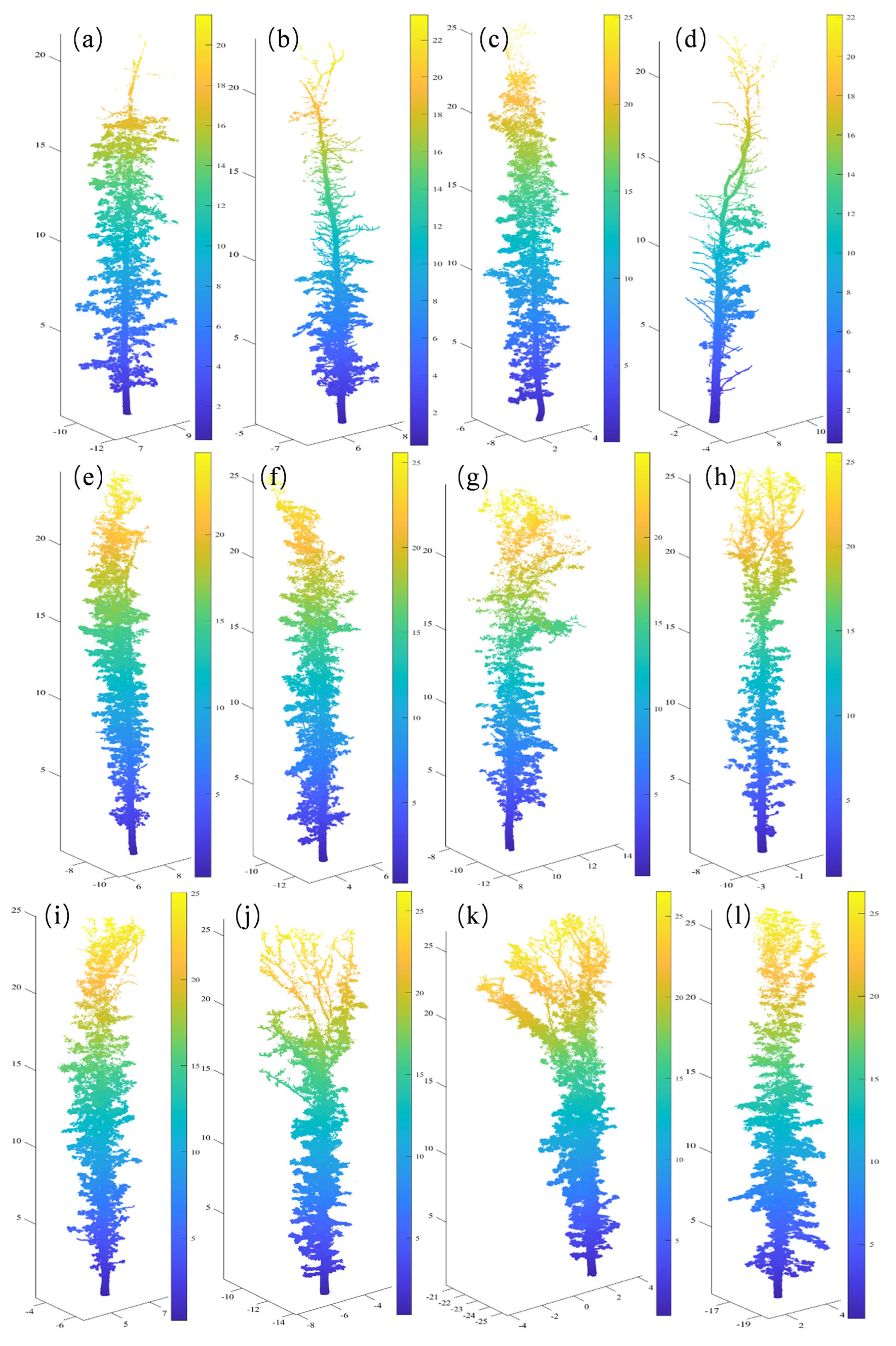
The original data obtained from the sample plot were subjected to denoising, ground point filtering, and height normalization. Ground points were obtained using an open-source cloth simulation filtering algorithm [60]. Normalization processing was carried out to eliminate the influence of terrain on the segmentation results of individual trees. The point cloud was processed using a comparative shortest-path algorithm (CSP) [61] combined with visual interpretation to obtain individual tree point clouds after height normalization. A total of 12 single-tree point cloud data were obtained for testing leaf and wood separation. This study categorized 12 single trees into linear and complex branch types. Detailed data can be found in Table 1, and the visualization of all single-tree point clouds is presented in Appendix A.

Table 1.
Summary of the single-tree point cloud data including branch type, number of points, tree height, diameter at breast height (DBH), and average point spacing.
Due to the instrument itself and the scanning environment, the acquired point cloud contained a large amount of noise, which was not effectively resolved during the denoising process of point cloud preprocessing. This could affect the calculation of point cloud geometric features and the construction of point cloud network diagrams, thus significantly influencing the leaf and branch separation. Therefore, this study proposes a layered adaptive voxel denoising method based on the uneven spatial density distribution of individual tree point clouds in the vertical direction. The process of this point cloud denoising method is shown in Figure 2. The method voxelizes point cloud slices of uniform thickness divided by elevation based on the average point spacing, which means the voxel size varies with the average point spacing. All voxels are traversed; if a current voxel is not empty and the total number of point clouds contained in the neighboring voxels (i.e., the surrounding 26 voxels) is less than or equal to 1, the points contained in the current voxel are considered noise. This method not only considers the uneven density of the point cloud in the vertical direction, but also takes into account the spatial arrangement of the noise data. Therefore, it can effectively remove noise data to more accurately segment leaf and non-leaf point clouds.
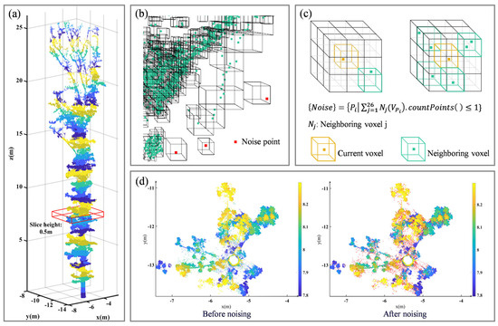
Figure 2.
Schematic of the layered adaptive voxel denoising method. (a) The point cloud of single trees is stratified with a layer thickness of 0.5 m (adjacent layers are represented by different colors), and the red box encloses a point cloud slice of 5.5–6 m. (b) A local magnified view of the voxels and denoising results from the slice at 5.5–6 m, where red indicates noise points, green indicates non-noise, and the black wireframe indicates voxels. (c) The principle of voxel denoising is that if the total number of points in the 26 neighboring voxels of a current non-empty voxel is less than or equal to 1, the points in the current voxel are considered to be noise. (d) A top-down comparison view of the slice at 5.5–6 m before and after denoising, where the red points represent noise.
2.2. Wood–Leaf Separation
This study proposes an unsupervised classification model (NE-PC) that combines point cloud geometric features and path detection algorithms, and the geometric features used in the study were determined to be valid in previous studies [29,62]. Specifically, our algorithm performs the following steps on the input single-tree point cloud: (1) supervoxel segmentation and supervoxel representative points extraction; (2) calculation of geometric features based on supervoxel and shortest-path tree construction by representative points; (3) optimization of node expansion detection for the trunk based on path frequency detection; (4) development of path concatenation detection of fine branches based on path retracing; (5) recovery of misclassified wood points and leaf points using a clustering filter to improve accuracy. The technical route of the NE-PC algorithm is shown in Figure 3.
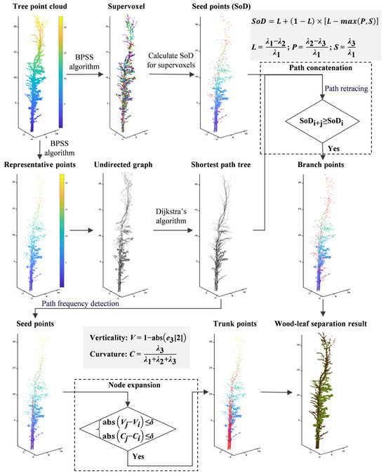
Figure 3.
The comprehensive technical route for the proposed wood–leaf separation method (NE-PC). The wood points identified by this method are a combination of wood points detected by path concatenation and node expansion (the red points in the figure), where the wood seed points for path concatenation are computed from the SoD features, and those for node expansion are detected by the path frequency. The points except for wood points in the single-tree point cloud are seen as the leaf points. Where the red dots indicate the detected wood nodes.
2.2.1. Constructing the Shortest-Path Tree for Single-Tree Point Clouds
Suppose a tree can be represented as a network structure where all nodes from the root to the leaves are connected. Paths with a higher frequency of occurrence, corresponding to the trunk and thicker branches, are detected by shortest path analysis. Constructing the network graph on a single-tree point cloud performing shortest path analysis is computationally complex and time-consuming. This study utilizes the boundary-preserved supervoxel segmentation (BPSS) on the point cloud. Each supervoxel contains only pure leaf points or pure wood points, meaning that a single supervoxel represents a small cluster of leaves or a segment of a branch. Using supervoxel representative points to construct the undirected graph significantly reduces the computational load compared to using the entire point cloud directly [45,63].
BPSS is a supervoxel segmentation method based on global energy optimization [64]. This algorithm employs an energy descent approach to transform the segmentation problem into a subset selection problem, where K representative points represent N points, and the subsets corresponding to these representative points constitute the segmented supervoxels. The algorithm comprises merge and exchange operations, as shown in Figure 4, eliminating the requirement for initializing seed points. It operates directly on the point cloud instead of working with voxels. The target function is as follows:
where the objective function E(Z) is formulated as an energy function, consisting of a feature distance constraint as the first term and a quantity constraint as the second term. The first term ensures that the selected representative points can effectively approximate the entire point set, while the second term constrains the number of representative points to be close to K. D(Pi, Pj) denotes the feature distance between points Pi and Pj [65]. N is the number of point clouds. Zij indicates that non-representative point Pj can be represented by representative point Pi, subject to Equations (2) and (3). C(Z) represents the number of representative points; K is the desired number of representative points, which can be calculated based on the supervoxel resolution R; and λ is a regularization parameter that balances the two terms, and its value is automatically evaluated using an adaptive strategy that accelerates optimization by leveraging local information [66]. The preliminary λ is set to the median of the minimum feature distances between neighboring points, and it is doubled in each subsequent iteration.
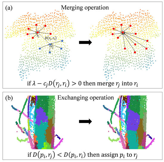
Figure 4.
Merge and exchange operations of the BPSS algorithm. (a) Merge operation of two adjacent representative points. (b) Result of exchange-based minimization. D represents the total dissimilarity distance, λ is a regularization parameter that balances the feature distance and the quantity constraint.
The merging criterion, where ∆ > 0, ensures that the merge operation occurs only if it reduces the overall energy function E(Z), thereby favoring configurations that minimize the energy. The adaptive strategy for λ adjustment enables the algorithm to balance the feature distance constraint and the quantity constraint dynamically, potentially enhancing the quality of supervoxel segmentations. It favors merging in smooth regions, such as those found on tree trunks.
where cj is the count of points within the supervoxel associated with representative point rj. The feature distance D(rj, ri) between representative points ri and rj is calculated using Equation (5), which specifies np and np as the normal vectors for p and q, respectively. R is the supervoxel resolution.
After identifying K representative points, an exchange operation is conducted for boundary points. These points are reassigned to the representative point with the shortest feature distance. For instance, if D(Pi, rj) < D(Pi, ri), then Pi is reassigned to the supervoxel associated with rj. This exchange operation refines the boundary definitions of supervoxels. More details about the BPSS algorithm are described in Algorithm A1 (Appendix B).
Constructing a connected network topology using supervoxel representative points derived from the point cloud offers advantages over graph construction with all points as nodes, including ease of implementation and lower computational complexity. In this method, the graph is denoted as G = (V, E), where V stands for the nodes, corresponding to the centroids of each supervoxel, and E is the set of edges connecting the adjacent supervoxels. To accurately represent the growth direction of trees, the point-to-point distance is assigned as the edge weight. The edge construction constraints are as follows:
where dist(Pi, Pj) is the Euclidean distance between Pi and Pj, with ds being the minimum threshold for edge construction.
The steps to construct the point cloud network structure graph are as follows:
- (1)
- Input the supervoxel representative points Q and the minimum elevation point d within all supervoxels.
- (2)
- Initialize an empty graph G.
- (3)
- Apply the k-nearest neighbors (KNN) algorithm to find n neighbors around each point in Q, recording their indices and distances r. Here, r is the Euclidean distance, with n set to 15.
- (4)
- Add all points in Q to graph G. Starting from d, use r as the weight and selectively add edges and their weights between each point in Q and the n neighbors found in step (3), following the constraint conditions.
- (5)
- Output the weighted topological network graph G.
After constructing the undirected graph, shortest path analysis is employed to identify the trunk and branches. Dijkstra’s algorithm [67] for single-source shortest paths calculates the shortest path from the lowest point to all other nodes in graph G, generating the shortest path tree.
2.2.2. Node Expansion for Trunk Detection
Given the growth structure of trees, the shortest paths from the lowest point to leaf nodes in the network graph follow the tree’s branches. Nodes along branches appear more frequently in the shortest-path tree than those in the leaves. By calculating the frequency of each node’s occurrence in all shortest paths within the tree, nodes with higher frequencies can be identified as wood nodes. This is expressed as follows:
where is the visit count of node Pi and max(log(f)) is the logarithm of the maximum visit count.
This process identifies wood seed nodes with visit counts greater than half of the logarithm of the highest visit count, detecting wood nodes on the main trunk and thicker branches. However, as shown in Figure 3, not all trunk and thicker branch nodes are identified, leading to a significant omission error. This is because shortest path analysis aims to find the minimum length path from the base point to a node, which may result in low visit frequencies for some trunk or branch nodes.
We propose a node expansion method based on geometric features to reduce the omission error. As shown in Figure 5, the main trunk and branches have relatively small verticality and curvature changes, while there are significant differences between the trunk and leaves. We optimize the detection of k neighboring points of wood nodes by expanding neighboring nodes with similar verticality and curvature to become wood nodes, as expressed in Equation (8):
where V and C represent the verticality and curvature of a node, respectively, and δ is a threshold set to 0.075. The verticality and curvature of each node are calculated based on the supervoxel it represents. Eigenvalues, representing data variability along orthogonal projection axes, are used to measure the spatial arrangement of point clouds. A covariance matrix for the supervoxel is constructed as shown in Equation (9):
where is the center of the segment and n is the total number of points in the segment. Principal component analysis (PCA) is used to calculate eigenvalues and eigenvectors for computing verticality and curvature features. Curvature is derived from the surface variation of the point set, and the methods for calculating verticality and curvature are given in Equation (10) [29,68]:
where λ1, λ2, and λ3 are the eigenvalues from PCA, with λ1 ≥ λ2 ≥ λ3, e3 is the eigenvector corresponding to λ3, e3 [2] is the third component of the eigenvector e3, and V and C represent the verticality and curvature features, respectively. More details are described in Table 2.
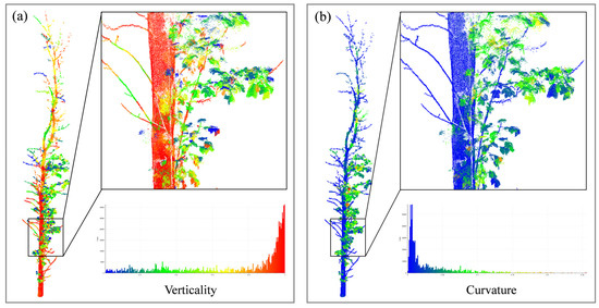
Figure 5.
Calculation of the verticality and curvature features based on supervoxels; different colors are plotted based on the geometric feature values. The figure’s bottom right corner displays the histogram of the point cloud features, with the horizontal coordinates of the histogram representing the magnitude of the feature values. (a) Verticality; (b) curvature.
Table 2.
Node expansion steps.
The neighborhood detection process for wood nodes can successfully identify the missed wood nodes.
2.2.3. Path Concatenation for Branch Detection
In path retracing algorithms, the characteristic that terminal nodes in the shortest-path tree often correspond to leaf vertices is utilized. The algorithm traces back from these terminal nodes, removing nodes to detect partial leaf nodes based on the number of retracing steps. Too many steps may overlook branches, while too few may under-detect leaf nodes. As shown in Appendix A, most leaf vertices are near-thin branches, and even terminal nodes have attached thin branches. Applying a uniform number of retracing steps across the shortest-path tree is challenging for distinguishing between branches and thin branch nodes. Therefore, this study proposes a path concatenation method based on salient features.
Salient features quantitatively describe the distribution of point sets, including linearity, planarity, and sphericity. A linearly distributed point set shows λ1 ≫ λ2 λ3, a planar distribution is characterized by λ1 λ2 ≫ λ3, and a spherically distributed set appears as λ1 λ2 λ3. Where λ1, λ2, and λ3 are derived from geometric characteristics computed using PCA. For each point within the supervoxel where the node resides, a covariance matrix is calculated, and eigenvalues λ1, λ2, and λ3 (where λ1 ≥ λ2 ≥ λ3) are obtained through singular value decomposition. Salient features are computed as per Equation (11) [25]:
where L, P, and S represent the linearity, planarity, and sphericity features, respectively, λ1, λ2, and λ3 are the eigenvalues from PCA.
As depicted in Figure 6, within a tree’s point cloud, trunks and branches generally exhibit dominant linear features, while leaves typically lack significant features, making direct detection based on leaf characteristics impractical. According to Figure 4, supervoxel segmentation divides the tree trunk into small segments, resulting in less pronounced linear salient features in the trunk area compared to branches and finer subdivisions, where these features are more evident. Thus, this study focuses on the linear features of branches. Firstly, wood seed nodes are identified among all nodes based on their linear characteristics. Then, using the shortest path, a backtrack is performed from the endpoint towards the base point, calculating the linear features of segments resulting from the merging of wood seed nodes with adjacent nodes. If the linear feature value of the merged segment is greater than that before merging, the adjacent node is added to the set of wood nodes.
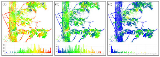
Figure 6.
Calculation of salient features based on supervoxels; different colors are plotted based on the geometric feature values. The figure’s bottom displays the histogram of the point cloud features, with the horizontal coordinates of the histogram representing the magnitude of the feature values. (a) Linearity; (b) planarity; (c) sphericity.
However, even when linear features share similar values, there can be variations in their saliency. To evaluate relative saliency levels, this study introduces the SoD index [29]. The SoD index is defined in Equation (12):
where L, P, and S represent the linearity, planarity, and sphericity features, respectively.
The SoD index ranges from −1 to 1. An SoD value less than 0 indicates that another salient feature is more prominent, while a value greater than 0 signifies that the linearity feature is more salient. A higher SoD value suggests a stronger linearity feature dominance. In this study, a threshold is used to detect wood nodes, with nodes having the SoD greater than identified as wood seed nodes; is set to 0.9 and is discussed further in Section 3.1.
The process of path concatenation is illustrated in Figure 3. For each shortest path from the shortest-path tree, we trace back from the endpoint to the base point. If a wood seed node is present, we concatenate it with adjacent nodes on the same path. We then calculate the SoD index of the concatenated segment to see if it exceeds the pre-merger SoD index. This aims to combine nodes on the same branch and identify wood nodes on the same path segment. More details are described in Table 3.
Table 3.
Path concatenation steps.
In merging the point clouds from node expansion and path concatenation, both subsets are branch point clouds, so their combination directly yields the wood nodes of the entire tree’s point cloud. To eliminate redundancy, duplicate points are removed post-merger. These wood nodes originate from supervoxel representative points. To obtain all branch points in the tree’s point cloud, each point is mapped to its supervoxel representative based on labels from supervoxel segmentation. This maps the wood nodes from the voxel space back to the original point cloud, yielding the entire tree’s branch point cloud.
2.2.4. Optimizing Wood–Leaf Separation Results Based on DBSCAN
Shortest path analysis, which seeks the minimum length path from the base to a node, may exclude some nodes on the same branch, leading to inaccuracies in path concatenation during retracing. To resolve this, we adapted a clustering filter inspired by Vicari et al. [41] to recover misclassified wood and leaf points.
Leveraging the fact that tree branch points in TLS point cloud data typically have a higher density than leaf points, we used the DBSCAN algorithm [69] for point cloud segmentation. DBSCAN identifies high-density clusters within a dataset. In 3D point clouds, for a point to be in a cluster, the number of points within a specified radius (eps) must meet or exceed a minimum count (MinPoints), signifying a neighborhood density above a set threshold.
We applied the DBSCAN clustering algorithm to the identified wood and leaf point clouds separately. Following a method similar to that used for calculating salient features, we computed the ratio of the maximum eigenvalue for each cluster. Clusters with a maximum eigenvalue ratio above 0.75 were retained to correct misclassified wood and leaf points.
2.3. Accuracy Assessment
To quantitatively evaluate the performance of our method for wood–leaf separation, this study uses CloudCompare software (version 2.12.4; Girardeau-Montaut, 2023, Blacksburg, VA, USA) to manually classify leaf and branch points as the ground truth. We employed three metrics: overall accuracy (OA), F1-score (F1), and kappa coefficient (kappa), to assess the wood–leaf separation results [70]. Additionally, we calculated Type I (T1) and Type II (T2) errors to further analyze classification inaccuracies [29,44].
where Tw is the number of correctly classified branch points, Fw is the number of incorrectly classified branch points, Tl is the number of correctly classified leaf points, and Fl is the number of incorrectly classified leaf points.
The F1-score, a harmonic mean of precision and recall, is used to validate the accuracy of leaf–branch separation. Precision, the proportion of correctly classified leaf points among all points classified as leaves, is calculated as follows:
Recall, the proportion of leaf points in the reference tree’s point cloud correctly classified as leaves, is as follows:
The F1-score is then as follows:
The kappa coefficient evaluates the consistency and accuracy of classification results, computed as follows:
where po is the observed agreement proportion and pe is the chance agreement probability, calculated as follows:
Type I error (T1), or omission error, is the ratio of incorrectly classified leaf points to the reference wood points; Type II error (T2), or commission error, is the ratio of incorrectly classified wood points to the reference leaf points. Their calculations are given by Equation (20) and Equation (21):
3. Experimental Results and Analysis
3.1. Sensitivity Analysis of Parameters
This study involves five key parameters: the resolution of supervoxels in BPSS R, the number of neighboring points in node expansion k, the threshold for verticality and curvature , the SoD threshold in path concatenation , and the DBSCAN parameter eps. The thresholds , , and eps were maintained as constant values throughout the study.
The threshold defines the dissimilarity in verticality and curvature between frequently visited trunk points and their neighboring points during node expansion; when this difference is less than or equal to , the neighboring point expands into a “wood node”. Consequently, must be sufficiently small to reflect the homogeneity in verticality and curvature among trunk points, as visually demonstrated in Figure 5 through the color-mapped point cloud distribution based on calculated verticality and curvature values. Therefore, this study fixes the threshold at 0.075. The threshold of the SoD index for identifying wood seed points during path retracing is specific to the study objects. A higher SoD index suggests a higher probability that a node is a wood point. As shown in Figure 7b, after supervoxel segmentation, fine branches are segmented into linear clusters, while the trunk forms planar clusters. Calculating the SoD index for the entire individual tree (based on the supervoxels containing the points) reveals that fine branches exhibit the highest SoD index, significantly differing from that of leaves. Considering the straight trunks and thin branches of the experimental tree samples (Figure 3), a threshold of 0.9 is deemed appropriate for detecting fine branch nodes. The parameter eps, serving as the crucial sensitivity threshold in DBSCAN clustering, was empirically optimized to 0.03 in this study. Excessive eps values (>0.03) were found to induce erroneous merges between fine twigs and surrounding leaf points during individual tree point cloud clustering, thereby compromising the algorithm’s capability to rectify misclassified points.
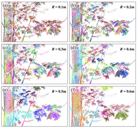
Figure 7.
Examples of supervoxels and representative points obtained using different expected resolutions of supervoxels, with different colors representing the supervoxel and red dots representing the supervoxel representative points. (a) R = 0.1 m; (b) R = 0.2 m; (c) R = 0.3 m; (d) R = 0.4 m; (e) R = 0.5 m; (f) R = 0.6 m.
To systematically evaluate the influence of parameters R (supervoxel resolution) and k (neighborhood size), experimental validation was conducted on Tree 4.
Figure 7 illustrates the supervoxel representative points for different R values (0.1, 0.2, 0.3, 0.4, 0.5, 0.6). Figure 8 demonstrates the shortest-path trees obtained under different supervoxel resolutions. The selection of R significantly influences the segmentation of supervoxels and the choice of representative points, thereby affecting the structure of the point cloud’s undirected graph and the shortest-path tree (composed of the shortest paths from each node to the base point). A small R results in a more detailed graph with a higher number of smaller supervoxels, while a large R simplifies the graph with fewer, larger supervoxels, potentially leading to classification errors by including both leaf and wood points within a single supervoxel. As R increases, the supervoxels become larger and fewer in number, potentially leading to under-segmentation, as illustrated in Figure 7f, while simultaneously introducing greater uncertainty in the generated shortest-path tree (Figure 8f). Conversely, reducing R results in a more complex network graph with an increased supervoxel count (Figure 7a), accompanied by a correspondingly higher complexity in the shortest-path tree structure (Figure 8a). According to the computational results in Figure 9, a larger value of R introduces greater uncertainty and a higher likelihood of misclassification, while reducing R does not always lead to improved classification accuracy. The experiments revealed that the shortest path analysis took more than three times longer when R = 0.1 m compared to R = 0.2 m. The results demonstrate that the highest classification accuracy was achieved when R was set to 0.2 m. Therefore, in this study, R was fixed at 0.2 m to ensure that each supervoxel exclusively contained either wood points or leaf points.

Figure 8.
Shortest-path trees generated from representative points under different supervoxel resolutions. (a) R = 0.1 m; (b) R = 0.2 m; (c) R = 0.3 m; (d) R = 0.4 m; (e) R = 0.5 m; (f) R = 0.6 m.

Figure 9.
Examples of shortest-path trees obtained using different expected resolutions of supervoxels.
The selection of k, the number of neighboring points for optimized detection during path frequency monitoring, is related to the size of supervoxels. As shown in Figure 7b, trunk points are divided into small clusters, with each corresponding to a supervoxel representative point that serves as a graph node. Since not all trunk nodes are detected by high visit counts during path frequency monitoring, node expansion is applied to identify wood seed points to enhance detection. This process relies on differences in curvature and verticality to successfully detect wood nodes on the same branch. A small k may miss some nodes within the same branch, while a large k can reduce algorithmic efficiency. Therefore, finding an appropriate k-value is crucial. Figure 10 presents the wood point detection results (recall, precision, and F1-scores of wood nodes) on Tree 4 using varying k-values (10, 20, 30, …, 100). To thoroughly analyze the sensitivity of k to wood point detection, the DBSCAN optimization process was intentionally disabled in the experiments. As shown, when the supervoxel resolution was fixed at 0.2 m, stable results were achieved for k ≥ 40 (F1-scores ranging from 0.935 to 0.937), whereas a resolution of 0.1 m required k ≥ 70 for stability (F1-scores: 0.913–0.918). This demonstrates that the optimal k must be adaptively determined based on R. Additionally, the precision of wood point detection remained highly stable (indicating a consistently high proportion of true wood points among the detected points), validating the algorithm’s effectiveness. Notably, the recall increased with larger k until saturation, implying that smaller k-values may omit valid wood points and reduce algorithmic efficiency. In this study, k was set to 40 based on the average breast-height diameter of the experimental tree samples and the size of the generated supervoxels, which was found to be optimal through experimentation.
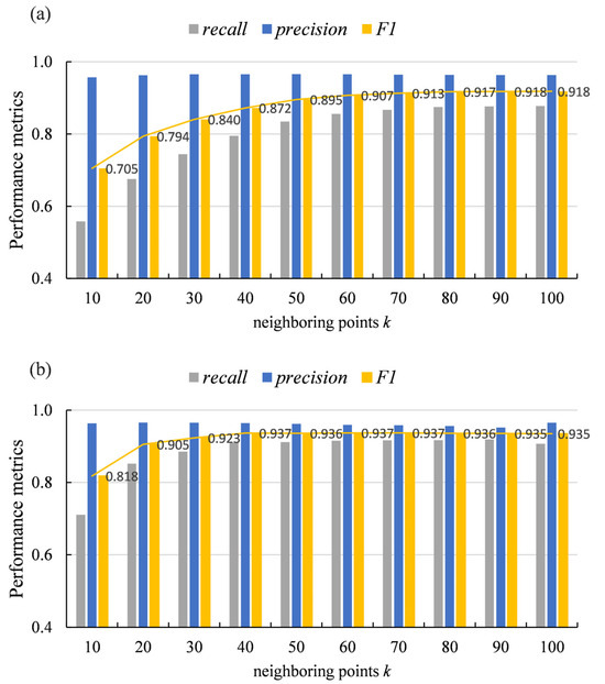
Figure 10.
Wood point detection results using different k-values, including recall, precision, and F1-score (the polyline represents F1-scores). (a) Results with fixed R = 0.1 m; (b) results with fixed R = 0.2 m.
3.2. Point-Wise Classification
To assess the effectiveness of the wood–leaf separation algorithm in this study, 12 single-tree point cloud datasets were utilized for result calculation, as detailed in Appendix A. These tree samples exhibited diverse morphological structures but shared common features: straight main trunks, numerous fine branches, and significant adhesion between leaves and branches. These characteristics rendered the data suitable for evaluating the detection capabilities of the proposed method for fine branch structures. Figure 11 displays the branch–leaf separation results of the proposed method, demonstrating its ability to identify the majority of main trunk points and its effectiveness in detecting fine branches.
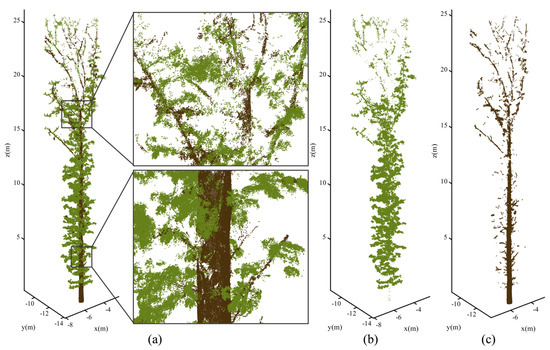
Figure 11.
Results of the wood and leaf separation proposed in this study. (a) Results of the branch and leaf separation and the local effect diagram; (b) point cloud of the leaves obtained from separation; (c) point cloud of the branches obtained from separation.
The accuracy metrics for the proposed method on two branch types (linear and complex) are presented in Table 4. The visualization of the wood and leaf separation results for 12 trees is presented in Appendix C. The method exhibits high performance on both branch types, with an average accuracy above 90%, an F1-score exceeding 0.9 for both wood and leaf points, and a kappa coefficient greater than 0.8. These results indicate that the method is effective in separating branches and leaves for single trees with various branch morphologies and consistently yields reliable separation results.
Table 4.
Calculation results of accuracy metrics for the proposed method on two types of branches.
To objectively assess the method proposed in this study, we conducted experiments using point cloud data from 12 individual trees. We compared our approach with two renowned wood–leaf separation approaches: TLSeparation [41] and LeWos [40]. LeWos employs recursive point cloud segmentation and regularization post-processing for wood–leaf separation. It segments the point cloud into clusters using a graph-based algorithm, distinguishing wood and leaf points based on cluster linearity. Regularization is then applied to refine the classification. LeWos offers both regularized and non-regularized results, with a single parameter controlling feature similarity, set to 0.15 following Wang et al.’s research. TLSeparation is a hybrid model that integrates machine learning classification with shortest path analysis for leaf–branch separation. It uses geometric features in a Gaussian mixture model (GMM) with the expectation–maximization (EM) algorithm for unsupervised classification and combines this with tree point cloud network graph analysis for branch point identification. TLSeparation requires several parameters, including neighborhood sizes and backtracking steps, using the default set provided by Vicari. LeWos and TLSeparation were selected for comparison because LeWos is a widely recognized open-source MATLAB (version R2022a, The MathWorks, Inc., 2022, Natick, MA, USA) tool, and TLSeparation provides comprehensive Python (version 3.9, Python Software Foundation, 2020, Wilmington, PA, USA) source code. Both methods use point cloud network graph construction for leaf–branch separation, facilitating a more objective comparative analysis.
We evaluated the proposed method using overall accuracy, F1-scores for wood and leaf points, and the kappa coefficient. The metrics for each tree are detailed in Table 5 and Figure 12, while Figure 13 presents a radar chart comparing the evaluation results of different methods across two branch types. The results show that our method achieved an accuracy above 90% for all 12 tree samples, with an overall accuracy of 94.1%, indicating effective wood–leaf separation. The average F1-scores for wood and leaf points exceeded 0.9, suggesting a balanced classification without over- or under-representing either category. The average kappa coefficient of 0.867 indicates a robust classification performance. Compared to other methods, our approach outperforms in accuracy, F1-scores, and the kappa coefficient, correctly classifying most tree point clouds into wood and leaf points with high separation performance. The method’s consistent performance across 12 single-tree point clouds of various morphologies demonstrates its strong generalization capability.
Table 5.
Comparison of evaluation indicators for 12 individual tree point clouds using the proposed method in this study, TLSeparation, and LeWos.

Figure 12.
Comparative analysis of evaluation indicators for wood and leaf separation using four methods. (a) Overall accuracy (OA); (b) kappa coefficient (kappa); (c) F1-score for wood point classification (F1-leaf); (d) F1-score for leaf point classification (F1-wood) [40,41].
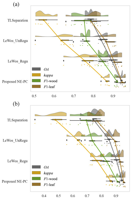
Figure 13.
Evaluation metrics for the separation of wood and leaves in linear and complex tree point clouds presented using a Raincloud plot [71]. These plots display the four quartiles, outliers (black prisms), and the median. Individual points denote the evaluation results for each single tree, with lines connecting the same evaluation metrics across different methods. (a) Test data—linear branch type; (b) test data—complex branch type.
The Type I and Type II errors for the four classification methods are detailed in Table 6. Our proposed method had the lowest average Type I error at 0.091, suggesting that it effectively detected wood points. The average Type II error for our method was 0.045, which is slightly higher than that of the regularized LeWoS. However, the Type I error of the regularized LeWoS was more than double that of our method. Our method better balanced Type I and Type II errors, with an average of 0.068 for both. In comparison, the non-regularized LeWoS had the Type I error over 10 times its Type II error, and the regularized LeWoS had the Type I error over 20 times its Type II error.
Table 6.
Comparison of the Type I and Type II errors across four methods of wood and leaf separation.
To visually assess the distribution of the Type I and Type II errors, this study presents error distribution diagrams for Tree 4 and Tree 10, two test samples with distinct branch types, as depicted in Figure 14. In the diagrams, correctly classified leaf points are indicated in green, incorrectly classified leaf points—in blue, correctly classified branch points—in brown, and incorrectly classified branch points—in yellow. Figure 14 demonstrates that our proposed method achieved the most effective wood–leaf classification, with a higher number of wood and leaf points correctly identified. Notably, in branch detection, our method outperformed the other three methods.
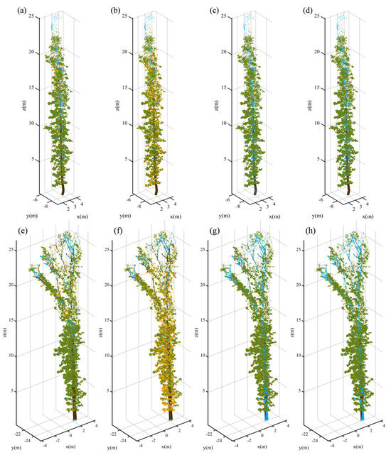
Figure 14.
Separation results of wood and leaf components for Tree 4 (linear type) and Tree 10 (complex type) using four methods. (a) Wood and leaf separation results for Tree 4 using the proposed NE-PC; (b) wood and leaf separation results for Tree 4 using TLSeparation; (c) wood and leaf separation results for Tree 4 using LeWos without regularization; (d) wood and leaf separation results for Tree 4 using LeWos with regularization; (e) wood and leaf separation results for Tree 10 using the proposed NE-PC; (f) wood and leaf separation results for Tree 10 using TLSeparation; (g) wood and leaf separation results for Tree 10 using LeWos without regularization; (h) wood and leaf separation results for Tree 10 using LeWos with regularization. Green represents the points correctly classified as leaves, blue represents the points incorrectly classified as leaves, brown represents the points correctly classified as branches, and yellow represents the points incorrectly classified as branches.
3.3. Validity of NE-PC
To further validate the effectiveness of the proposed NE-PC method, we acquired additional point clouds of Liriodendron × sino-americanum forests from Xiashu Forest Farm in Zhenjiang, Jiangsu Province (Plot B), and Lishan Forest Farm in Ji’an, Jiangxi Province (Plot C). A total of 11 single-tree point clouds were randomly selected (Plot B: 6 trees; Plot C: 5 trees) for testing and pointwise accuracy validation. Although these 11 samples belonged to the same species as the 12 trees in Section 2.1 (Nanjing Forestry University Arboretum: Plot A), their architectures exhibited significant variations due to environmental and silvicultural factors. Compared to Plot A, trees in Plot B featured a denser leaf–wood point adhesion, with substantial leaf attachments even on trunks, while trees in Plot C displayed fuller crowns and more complex branching structures. Selection of these structurally divergent samples rigorously tested the method’s applicability across heterogeneous tree morphologies.
The proposed method was executed with identical wood–leaf separation parameters across all three plots (A, B, C). Quantitative metrics are presented in Table 7, and visual comparisons are provided in Figure 15. The NE-PC method achieved consistent classification performance on these 11 trees, mirroring results from Plot A: average overall accuracy (OA) > 90%, mean kappa coefficient > 0.8, leaf point F1-scores > 0.9, and wood point F1-scores > 0.8. Type I error analysis revealed that misclassified leaf points (primarily concentrated in upper crowns, as observed in the experimental samples) were the main factor limiting wood point F1-scores, indicating partial under-detection of woody components. Increased architectural complexity exacerbated classification uncertainty in upper canopies. Nevertheless, Figure 15 demonstrates successful extraction of continuous branch point clouds, providing a robust foundation for subsequent tree modeling applications.
Table 7.
Wood–leaf separation evaluation metrics of the trees from plots A, B, and C using the NE-PC method.
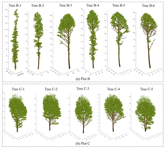
Figure 15.
Leaf–wood separation results for the trees from plots B and C using the NE-PC method.
4. Discussion
4.1. Parameter Analysis
This paper focuses on five key parameters: the supervoxel resolution R in the BPSS algorithm, the number of neighborhood points k for optimized detection in path frequency monitoring, the threshold for verticality and curvature , the threshold ξ of the SoD index for identifying wood seed points during path retracing, and the DBSCAN parameter eps. The thresholds and eps were set as constant values throughout the study, while R, k, and could be appropriately adjusted according to the following rules. The choice of R influences the segmentation of supervoxels, affecting the representative points and classification accuracy. A smaller R yields more detailed segments and a more complex graph, potentially reducing algorithm efficiency. Therefore, R can be determined based on factors such as leaf size and point density in the experimental samples. The number of neighborhood points k is related to the size of supervoxels, which, in turn, depends on R. A larger R results in fewer supervoxel points, suggesting a reduction in k. Conversely, a smaller R generates more supervoxel points, indicating an increase in k. The threshold ξ of the SoD index for identifying wood seed points is specific to the experiment’s research object. A higher SoD index indicates a higher likelihood of a node being a wood point. If the experimental samples have thicker branches and a low frequency of fine branches, ξ can be adjusted to enhance the detection of wood points.
4.2. Point-Wise Classification
We tested the NE-PC algorithm on point clouds from 12 structurally complex individual trees. Comparing the four classification methods (LeWos_unregu, LeWos_regu, TLSeparation, and our proposed method) using the metrics from Table 5 and Figure 12, we conducted a comparative analysis of the overall accuracy, kappa coefficient, wood point F1-score, and leaf point F1-score. Our method outperformed LeWos and TLSeparation in the overall classification accuracy, with an average of 94.1% across all datasets. The regularized LeWos also showed better performance than the non-regularized version. In terms of the wood point F1-score, our method achieved the highest score across all samples, with all but Tree 1 exceeding an F1-score of 0.9, and Tree 1’s score was still higher than that achieved with the other methods. For the leaf point F1-score, our method surpassed LeWos in all samples. The kappa coefficient for our method was above 0.8 in all cases, indicating no systematic tendency to misclassify leaf points as wood points or wood points as leaf points. The error distribution diagram (Figure 14) demonstrates that NE-PC achieved the most complete stem point detection among the three compared methods, with superior capability in identifying fine branch points that are adherent to leaf points. The NE-PC algorithm was additionally evaluated for individual tree leaf–wood separation in structurally complex Plot B and Plot C, yielding classification accuracies of 92.8% and 94.4%, respectively, with the mean kappa coefficients surpassing 0.8. In contrast to these 12 tree point clouds, the samples from Plot B exhibited richer fine-branch structures and denser foliage, while those from Plot C display fuller crowns and more complex branching patterns, particularly Tree C-5 with its multiple trunks. The algorithm maintained excellent wood–leaf separation performance across various foliage densities and trunk architectures, demonstrating NE-PC’s robustness and generalizability to diverse tree structural morphologies.
The method proposed in this study achieves comparable separation results to prior approaches across different datasets. Ma et al. [25] employed a supervised Gaussian mixture model (GMM) based on salient features to separate foliage and wood components from TLS data of forest canopies, reporting overall accuracies of 93.09% for broadleaf and 94.96% for coniferous trees. Zhou et al. [28] introduced a Multi-Optimal-Scale Method for distinguishing leaf and wood points in tree point clouds, achieving an overall accuracy of 91.81%, representing a 1–3% improvement over single-scale approaches. Wan et al. [29] proposed a segment-based classification strategy for separating wood and leaf points from TLS data in forest plots, reporting total error rates of 5.39–7.76% and kappa coefficients of 77.11–81.19% across multiple forest sites and open datasets. Sun et al. [36] developed an automated method combining intensity and geometric features for leaf–wood classification in tree point clouds, with experimental results on 24 willow trees showing the overall accuracy (OA) ranging from 0.9167 to 0.9872, kappa coefficients—from 0.7276 to 0.9191. Hui et al. [44] introduced a pattern point evolution-based method for wood and leaf separation, achieving a mean classification accuracy of 0.892, with average F1-scores of 0.871 for wood and 0.900 for foliage across nine tree species. Lu et al. [43] proposed a hybrid approach integrating shortest-path analysis and graph segmentation for branch–leaf separation, demonstrating robustness in handling incomplete fine branch extraction with classification accuracies of 0.9697, 0.9469, and 0.9314 on open datasets of varying point densities, along with kappa coefficients consistently exceeding 0.84. Tian et al. [42] developed a graph-based wood–leaf separation (GBS) method that utilizes only the xyz coordinates of point clouds for individual tree classification. The proposed approach was evaluated using data from 10 different tree species, demonstrating an average accuracy of 94% and a kappa coefficient of 0.78. Recent deep learning-based methods have also shown strong performance. Van den Broeck et al. [50] applied RandLA-Net, a 3D deep learning architecture, to tropical tree point clouds, achieving a mean intersection-over-union (mIoU) of 86.8% and an overall accuracy of 94.8% across 148 trees. Dai et al. [51] introduced a multi-directional collaborative convolutional neural network (MDC-Net) for leaf–wood separation in TLS forest point clouds, reporting an overall accuracy of 0.973 and an mIoU of 0.821 in experiments conducted across five forest plots in Guangxi. Xi et al. [47] earlier utilized a 3D fully convolutional network (FCN) for trunk and branch filtering from TLS data, obtaining an average IoU of 0.79 and an overall accuracy of 0.94 in single-tree analysis.
The processing time recorded for wood–leaf separation across all tree point clouds (Appendix D) indicates that the time required to process a single tree ranges from 1 to 5 min, with approximately 60–90 s per 1 million points. In comparison, TLSeparation takes around 10 min per 1 million points, while LeWos requires about 90 s per 1 million points, which aligns with the conclusions reported by their respective authors. Our algorithm demonstrates a higher efficiency than TLSeparation and matches the computational speed of LeWos.
A supervoxel-based classification method is proposed in this study to handle individual tree point clouds characterized by high point density, large data volumes, and intricate structural complexity. In contrast to other supervised learning approaches that require extensive manually labeled point cloud data for training, the proposed method utilizes only the coordinate information of the point clouds. The method includes node expansion to counteract the omission of trunk points by path frequency detection, ensuring stable trunk point identification. Additionally, the path concatenation method emphasizes the geometric characteristics of fine branches and integrates path retracing to enhance the detection of fine branches, thus improving the accuracy of wood–leaf separation.
Figure 14’s error distribution diagram shows our method’s errors are concentrated above the canopy. As per Table 1, tree heights ranged from 21.5 m to 26.5 m, and scanning occlusions led to unclear point clouds above the canopy, affecting detection. Data quality serves as a prerequisite for the successful classification of wood and leaf points [41]. However, the challenge of data acquisition becomes more severe in environments with high stand density and complex, heavily occluded canopies. Data quality depends on multiple factors, including the specifications of the acquisition device, scanning setup, registration accuracy, and canopy occlusion severity. These challenges can be partially mitigated by utilizing high-resolution laser scanners, implementing optimized scanning schemes, and refining registration methods [59].
Another key challenge in wood–leaf classification algorithms is achieving an optimal trade-off between the Type I and Type II errors, defined as the ratio of misclassified wood points to the total reference wood points (Type I) and the ratio of misclassified leaf points to the total reference leaf points (Type II). While the overall accuracy and kappa coefficient are standard evaluation metrics, practical forestry applications require careful consideration of both error types and their balance [72,73]. For example, in tree volume or aboveground biomass (AGB) estimation, elevated Type II errors significantly contribute to overestimation. Notably, Type I errors predominantly occur in small branches due to their morphological similarity to leaves, yet their limited volumetric contribution minimizes the impact on wood volume calculations. Conversely, quantitative characterization of branch architecture demands algorithms with minimal Type I errors, whereas canopy structural analysis (e.g., leaf area index and porosity estimation) requires balanced error types to ensure unbiased results. Experimental results demonstrate that our proposed method achieves superior performance with simultaneously reduced Type I and Type II errors, and our method balances Type I and Type II errors effectively, avoiding misclassification in both directions.
The method proposed in this study can improve the recognition rate of wood components, especially the components of small branches, and achieved excellent classification results on the point clouds of 23 trees with high density and complex branching structures from different forest plots. However, according to previous studies, significant changes in point density may affect the recognition of wood points [30,37]. In the future, the proposed method needs to be further tested and examined on data with other point densities. Furthermore, all individual tree samples used in this study were Liriodendron × sino-americanum, although they exhibited various architectural forms. The method’s performance on data from other tree species with different scanning protocols, point cloud qualities, growth morphologies, and forest environments warrants further evaluation.
5. Conclusions
This study proposed an advanced model (NE-PC) for separating wood and leaf components from point clouds by integrating geometric features and network graph analysis. The classification accuracy for wood–leaf separation in point clouds of 12 individual Liriodendron × sino-americanum trees reached 94.1% (± 2.1%), with a kappa coefficient of 86.7% (± 3.4%). Our algorithm combines path frequency detection and node expansion to effectively identify missed wood nodes on trunks and branches. The proposed path concatenation detection algorithm in the path retracing phase successfully identifies wood nodes on the same branch. A clustering filter is then applied to correct misclassified points, enhancing the algorithm’s ability to separate leaves and branches. Compared to the TLSeparation method, our approach shows better performance in detecting both trunk and branch points completely (ΔF1-wood = 8.7–32.7%, ΔF1-leaf = 12.4–26.2%). Compared to the LeWos method, our method demonstrates improved detection performance for fine branches (ΔF1-wood = 4.7–10.7%, ΔF1-leaf = 1.1–13.4%). The NE algorithm was further evaluated on 11 individual Liriodendron × sino-americanum trees featuring distinct crown architectures within Plot A and Plot B. The mean overall accuracy (OA) exceeded 90% in both plots (Plot A: 92.8 ± 2.3%; Plot B: 94.4 ± 0.7%), with the mean kappa coefficients consistently above 80% (Plot A: 81.3 ± 4.2%; Plot B: 81.8 ± 3.2%). These results demonstrate the algorithm’s adaptability to various crown structure types. The separation results provide a valuable reference for subsequent individual tree analysis applications.
Author Contributions
Conceptualization, L.C.; methodology, S.G. and X.S.; software, S.G. and X.S.; validation, S.G. and X.S.; formal analysis, S.G.; writing—original draft preparation, S.G.; writing—review and editing, S.G., X.S. and L.C.; visualization, S.G.; supervision, L.C.; funding acquisition, X.S. and L.C. All authors have read and agreed to the published version of the manuscript.
Funding
This research was funded by the National Key Research and Development Program (2022YFD2200101), the Natural Science Foundation of Jiangsu Province (BK20220415), and the Priority Academic Program Development of Jiangsu Higher Education Institutions (PAPD).
Data Availability Statement
Data are contained within the article.
Acknowledgments
We gratefully acknowledge graduate students from the Department of Forest Management at Nanjing Forestry University for field work.
Conflicts of Interest
The authors declare no conflicts of interest.
Appendix A
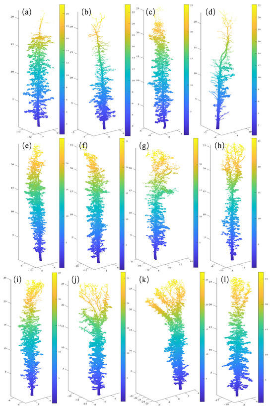
Figure A1.
Datasets used for the testing. (a) Tree 1; (b) Tree 2; (c) Tree 3; (d) Tree 4; (e) Tree 5; (f) Tree 6; (g) Tree 7; (h) Tree 8; (i) Tree 9; (j) Tree 10; (k) Tree 11; (l) Tree 12.
Figure A1.
Datasets used for the testing. (a) Tree 1; (b) Tree 2; (c) Tree 3; (d) Tree 4; (e) Tree 5; (f) Tree 6; (g) Tree 7; (h) Tree 8; (i) Tree 9; (j) Tree 10; (k) Tree 11; (l) Tree 12.
Appendix B
| Algorithm A1. BPSS |
| Input: point cloud, , neighborhood, , target resolution, R. Output: representative points, , labels L 1: Initialize 2: Merge operation: 3: while > K do 4: for each adjacent pair ( do 5: compute according Equation (4) 6: if > 0 then 7: 8: Update 9: 10: end while 11: Exchange operation: 12: for each boundary point do 13: find argmin_{} 14: If then 15: 16: end for |
represents the volume of the point cloud’s bounding box and K is initialized by calculating the number of points after voxel-grid down-sampling at a given resolution R. D denotes the feature distance, computed using Equation (5). The merging operation minimizes the energy function while searching for K supervoxel representative points; represents a boundary point, meaning that the label of differs from that of at least one of its neighboring points; denotes the point closest to . The exchange operation reassigns new labels to qualifying boundary points, resulting in the final supervoxel labels.
Appendix C
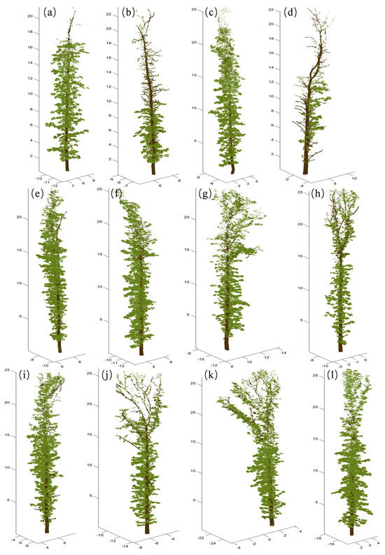
Figure A2.
Wood–leaf separation results. (a) Tree 1; (b) Tree 2; (c) Tree 3; (d) Tree 4; (e) Tree 5; (f) Tree 6; (g) Tree 7; (h) Tree 8; (i) Tree 9; (j) Tree 10; (k) Tree 11; (l) Tree 12.
Figure A2.
Wood–leaf separation results. (a) Tree 1; (b) Tree 2; (c) Tree 3; (d) Tree 4; (e) Tree 5; (f) Tree 6; (g) Tree 7; (h) Tree 8; (i) Tree 9; (j) Tree 10; (k) Tree 11; (l) Tree 12.

Appendix D
Table A1.
Processing time for the leaf–wood separation algorithm testing using tree point clouds from plots A, B, and C.
Table A1.
Processing time for the leaf–wood separation algorithm testing using tree point clouds from plots A, B, and C.
| Plot | Tree ID | No. of Points | Height (m) | Processing Time (s) |
|---|---|---|---|---|
| Plot A | TreeA-1 | 597,399 | 21.5 | 90.95 |
| TreeA-2 | 632,257 | 23.4 | 31.59 | |
| TreeA-3 | 664,178 | 25.1 | 30.32 | |
| TreeA-4 | 717,921 | 22.1 | 60.05 | |
| TreeA-5 | 766,925 | 24.7 | 36.60 | |
| TreeA-6 | 952,533 | 25.6 | 45.30 | |
| TreeA-7 | 586,990 | 25 | 107.34 | |
| TreeA-8 | 723,175 | 25.6 | 35.47 | |
| TreeA-9 | 963,192 | 25.1 | 75.09 | |
| TreeA-10 | 1,495,627 | 26.2 | 107.49 | |
| TreeA-11 | 1,633,618 | 26.5 | 119.45 | |
| TreeA-12 | 1,911,356 | 26.3 | 94.47 | |
| Plot B | TreeB-1 | 1,166,361 | 18.7 | 64.00 |
| TreeB-2 | 900,975 | 17.2 | 53.83 | |
| TreeB-3 | 1,593,612 | 19.3 | 148.35 | |
| TreeB-4 | 1,326,197 | 18 | 87.93 | |
| TreeB-5 | 931,088 | 17.4 | 67.68 | |
| TreeB-6 | 836,643 | 16.5 | 47.99 | |
| Plot C | TreeC-1 | 3,243,740 | 12.2 | 245.96 |
| TreeC-2 | 3,421,306 | 11.8 | 233.73 | |
| TreeC-3 | 2,222,633 | 11.6 | 145.19 | |
| TreeC-4 | 2,085,081 | 10.5 | 125.89 | |
| TreeC-5 | 3,354,258 | 11.1 | 234.27 |
References
- Beland, M.; Parker, G.; Sparrow, B.; Harding, D.; Chasmer, L.; Phinn, S.; Antonarakis, A.; Strahler, A. On promoting the use of lidar systems in forest ecosystem research. For. Ecol. Manag. 2019, 450, 117484. [Google Scholar] [CrossRef]
- Disney, M.I.; Vicari, M.B.; Burt, A.; Calders, K.; Lewis, S.L.; Raumonen, P.; Wilkes, P. Weighing trees with lasers: Advances, challenges and opportunities. Interface Focus. 2018, 8, 20170048. [Google Scholar] [CrossRef] [PubMed]
- Ehbrecht, M.; Schall, P.; Ammer, C.; Seidel, D. Quantifying stand structural complexity and its relationship with forest management, tree species diversity and microclimate. Agric. For. Meteorol. 2017, 242, 1–9. [Google Scholar] [CrossRef]
- Terryn, L.; Calders, K.; Bartholomeus, H.; Bartolo, R.E.; Brede, B.; D’Hont, B.; Disney, M.; Herold, M.; Lau, A.; Shenkin, A.; et al. Quantifying tropical forest structure through terrestrial and UAV laser scanning fusion in Australian rainforests. Remote Sens. Environ. 2022, 271, 112912. [Google Scholar] [CrossRef]
- Wang, Y.; Lehtomäki, M.; Liang, X.; Pyörälä, J.; Kukko, A.; Jaakkola, A.; Liu, J.; Feng, Z.; Chen, R.; Hyyppä, J. Is field-measured tree height as reliable as believed—A comparison study of tree height estimates from field measurement, airborne laser scanning and terrestrial laser scanning in a boreal forest. Isprs-J. Photogramm. Remote Sens. 2019, 147, 132–145. [Google Scholar] [CrossRef]
- Calders, K.; Adams, J.; Armston, J.; Bartholomeus, H.; Bauwens, S.; Bentley, L.P.; Chave, J.; Danson, F.M.; Demol, M.; Disney, M.; et al. Terrestrial laser scanning in forest ecology: Expanding the horizon. Remote Sens. Environ. 2020, 251, 112102. [Google Scholar] [CrossRef]
- Disney, M. Terrestrial LiDAR: A three-dimensional revolution in how we look at trees. New Phytol. 2019, 222, 1736–1741. [Google Scholar] [CrossRef]
- Yrttimaa, T.; Luoma, V.; Saarinen, N.; Kankare, V.; Junttila, S.; Holopainen, M.; Hyyppä, J.; Vastaranta, M. Structural Changes in Boreal Forests Can Be Quantified Using Terrestrial Laser Scanning. Remote Sens. 2020, 12, 2672. [Google Scholar] [CrossRef]
- Chianucci, F.; Puletti, N.; Grotti, M.; Ferrara, C.; Giorcelli, A.; Coaloa, D.; Tattoni, C. Nondestructive Tree Stem and Crown Volume Allometry in Hybrid Poplar Plantations Derived from Terrestrial Laser Scanning. For. Sci. 2020, 66, 737–746. [Google Scholar] [CrossRef]
- Li, Y.; Hess, C.; von Wehrden, H.; Hardtle, W.; von Oheimb, G. Assessing tree dendrometrics in young regenerating plantations using terrestrial laser scanning. Ann. For. Sci. 2014, 71, 453–462. [Google Scholar] [CrossRef]
- Demol, M.; Verbeeck, H.; Gielen, B.; Armston, J.; Burt, A.; Disney, M.; Duncanson, L.; Hackenberg, J.; Kukenbrink, D.; Lau, A.; et al. Estimating forest above-ground biomass with terrestrial laser scanning: Current status and future directions. Methods Ecol. Evol. 2022, 13, 1628–1639. [Google Scholar] [CrossRef]
- Kükenbrink, D.; Gardi, O.; Morsdorf, F.; Thürig, E.; Schellenberger, A.; Mathys, L. Above-ground biomass references for urban trees from terrestrial laser scanning data. Ann. Bot. 2021, 128, 709–724. [Google Scholar] [CrossRef] [PubMed]
- Disney, M.; Burt, A.; Calders, K.; Schaaf, C.; Stovall, A. Innovations in Ground and Airborne Technologies as Reference and for Training and Validation: Terrestrial Laser Scanning (TLS). Surv. Geophys. 2019, 40, 937–958. [Google Scholar] [CrossRef]
- Chen, Y.M.; Zhang, W.M.; Hu, R.H.; Qi, J.B.; Shao, J.; Li, D.; Wan, P.; Qiao, C.; Shen, A.J.; Yan, G.J. Estimation of forest leaf area index using terrestrial laser scanning data and path length distribution model in open-canopy forests. Agric. For. Meteorol. 2018, 263, 323–333. [Google Scholar] [CrossRef]
- Zheng, G.; Moskal, L.M. Computational-Geometry-Based Retrieval of Effective Leaf Area Index Using Terrestrial Laser Scanning. IEEE Trans. Geosci. Remote Sens. 2012, 50, 3958–3969. [Google Scholar] [CrossRef]
- Liu, J.; Wang, T.J.; Skidmore, A.K.; Jones, S.; Heurich, M.; Beudert, B.; Premier, J. Comparison of terrestrial LiDAR and digital hemispherical photography for estimating leaf angle distribution in European broadleaf beech forests. ISPRS-J. Photogramm. Remote Sens. 2019, 158, 76–89. [Google Scholar] [CrossRef]
- Li, Y.; Guo, Q.; Tao, S.; Zheng, G.; Zhao, K.; Xue, B.; Su, Y. Derivation, Validation, and Sensitivity Analysis of Terrestrial Laser Scanning-Based Leaf Area Index. Can. J. Remote Sens. 2016, 42, 719–729. [Google Scholar] [CrossRef]
- Yan, G.; Hu, R.; Luo, J.; Mu, X.; Xie, D.; Zhang, W. Review of indirect methods for leaf area index measurement. J. Remote Sens. 2016, 20, 958–978. [Google Scholar]
- Zhu, X.; Skidmore, A.K.; Wang, T.; Liu, J.; Darvishzadeh, R.; Shi, Y.; Premier, J.; Heurich, M. Improving leaf area index (LAI) estimation by correcting for clumping and woody effects using terrestrial laser scanning. Agric. For. Meteorol. 2018, 263, 276–286. [Google Scholar] [CrossRef]
- Kankare, V.; Holopainen, M.; Vastaranta, M.; Puttonen, E.; Yu, X.; Hyyppä, J.; Vaaja, M.; Hyyppä, H.; Alho, P. Individual tree biomass estimation using terrestrial laser scanning. ISPRS-J. Photogramm. Remote Sens. 2013, 75, 64–75. [Google Scholar] [CrossRef]
- Chen, S.; Verbeeck, H.; Terryn, L.; Van den Broeck, W.A.J.; Vicari, M.B.; Disney, M.; Origo, N.; Wang, D.; Xi, Z.; Hopkinson, C.; et al. The impact of leaf-wood separation algorithms on aboveground biomass estimation from terrestrial laser scanning. Remote Sens. Environ. 2025, 318, 114581. [Google Scholar] [CrossRef]
- Arseniou, G.; MacFarlane, D.W.; Calders, K.; Baker, M. Accuracy differences in aboveground woody biomass estimation with terrestrial laser scanning for trees in urban and rural forests and different leaf conditions. Trees-Struct. Funct. 2023, 37, 761–779. [Google Scholar] [CrossRef]
- Liang, X.; Hyyppä, J.; Kaartinen, H.; Lehtomäki, M.; Pyörälä, J.; Pfeifer, N.; Holopainen, M.; Brolly, G.; Francesco, P.; Hackenberg, J.; et al. International benchmarking of terrestrial laser scanning approaches for forest inventories. ISPRS-J. Photogramm. Remote Sens. 2018, 144, 137–179. [Google Scholar] [CrossRef]
- Liang, X.; Kankare, V.; Hyyppä, J.; Wang, Y.; Kukko, A.; Haggrén, H.; Yu, X.; Kaartinen, H.; Jaakkola, A.; Guan, F.; et al. Terrestrial laser scanning in forest inventories. ISPRS-J. Photogramm. Remote Sens. 2016, 115, 63–77. [Google Scholar] [CrossRef]
- Ma, L.; Zheng, G.; Eitel, J.U.H.; Moskal, L.M.; He, W.; Huang, H. Improved Salient Feature-Based Approach for Automatically Separating Photosynthetic and Nonphotosynthetic Components Within Terrestrial Lidar Point Cloud Data of Forest Canopies. IEEE Trans. Geosci. Remote Sens. 2016, 54, 679–696. [Google Scholar] [CrossRef]
- Wang, D.; Hollaus, M.; Pfeifer, N. Feasibility of machine learning methods for separating wood and leaf points from terrestrial laser scanning data. ISPRS Ann. Photogramm. Remote Sens. Spat. Inf. Sci. 2017, IV-2/W4, 157–164. [Google Scholar] [CrossRef]
- Wang, Z.; Zhang, L.; Fang, T.; Mathiopoulos, P.T.; Tong, X.; Qu, H.; Xiao, Z.; Li, F.; Chen, D. A multiscale and hierarchical feature extraction method for terrestrial laser scanning point cloud classification. IEEE Trans. Geosci. Remote Sens. 2015, 53, 2409–2425. [Google Scholar] [CrossRef]
- Zhou, J.; Wei, H.; Zhou, G.; Song, L. Separating leaf and wood points in terrestrial laser scanning data using multiple optimal scales. Sensors 2019, 19, 1852. [Google Scholar] [CrossRef]
- Wan, P.; Shao, J.; Jin, S.; Wang, T.; Yang, S.; Yan, G.; Zhang, W. A novel and efficient method for wood-leaf separation from terrestrial laser scanning point clouds at the forest plot level. Methods Ecol. Evol. 2021, 12, 2473–2486. [Google Scholar] [CrossRef]
- Ferrara, R.; Virdis, S.G.P.; Ventura, A.; Ghisu, T.; Duce, P.; Pellizzaro, G. An automated approach for wood-leaf separation from terrestrial LIDAR point clouds using the density based clustering algorithm DBSCAN. Agric. For. Meteorol. 2018, 262, 434–444. [Google Scholar] [CrossRef]
- Wang, M.; Wong, M.S. A novel geometric feature-based wood-leaf separation method for large and crown-heavy tropical trees using handheld laser scanning point cloud. Int. J. Remote Sens. 2023, 44, 3227–3258. [Google Scholar] [CrossRef]
- Yun, T.; An, F.; Li, W.; Sun, Y.; Cao, L.; Xue, L. A Novel Approach for Retrieving Tree Leaf Area from Ground-Based LiDAR. Remote Sens. 2016, 8, 942. [Google Scholar] [CrossRef]
- Moorthy, S.M.K.; Calders, K.; Vicari, M.B.; Verbeeck, H. Improved Supervised Learning-Based Approach for Leaf and Wood Classification From LiDAR Point Clouds of Forests. IEEE Trans. Geosci. Remote Sens. 2020, 58, 3057–3070. [Google Scholar] [CrossRef]
- Béland, M.; Baldocchi, D.D.; Widlowski, J.; Fournier, R.A.; Verstraete, M.M. On seeing the wood from the leaves and the role of voxel size in determining leaf area distribution of forests with terrestrial LiDAR. Agric. For. Meteorol. 2014, 184, 82–97. [Google Scholar] [CrossRef]
- Sun, Y.; Lin, X.; Xiong, J.; Ren, G. Separation of single wood branches and leaves based on corrected TLS intensity data. Chin. J. Lasers 2021, 48, 104001. [Google Scholar] [CrossRef]
- Sun, J.; Wang, P.; Gao, Z.; Liu, Z.; Li, Y.; Gan, X.; Liu, Z. Wood–leaf classification of tree point cloud based on intensity and geometric information. Remote Sens. 2021, 13, 4050. [Google Scholar] [CrossRef]
- Tan, K.; Zhang, W.; Dong, Z.; Cheng, X.; Cheng, X. Leaf and wood separation for individual trees using the intensity and density data of terrestrial laser scanners. IEEE Trans. Geosci. Remote Sens. 2021, 59, 7038–7050. [Google Scholar] [CrossRef]
- Shao, J.Y.; Cheng, Y.T.; Koshan, Y.; Manish, R.; Habib, A.; Fei, S.L. Radiometric and geometric approach for major woody parts segmentation in forest lidar point clouds. In Proceedings of the IGARSS 2023-2023 IEEE International Geoscience and Remote Sensing Symposium, Pasadena, CA, USA, 16–21 July 2023; pp. 6220–6223. [Google Scholar]
- Tao, S.; Guo, Q.; Su, Y.; Xu, S.; Li, Y.; Wu, F. A geometric method for wood-leaf separation using terrestrial and simulated lidar data. Photogramm. Eng. Remote Sens. 2015, 81, 767–776. [Google Scholar] [CrossRef]
- Wang, D.; Momo Takoudjou, S.; Casella, E. LeWoS: A universal leaf-wood classification method to facilitate the 3D modelling of large tropical trees using terrestrial LiDAR. Methods Ecol. Evol. 2020, 11, 376–389. [Google Scholar] [CrossRef]
- Vicari, M.B.; Disney, M.; Wilkes, P.; Burt, A.; Calders, K.; Woodgate, W. Leaf and wood classification framework for terrestrial LiDAR point clouds. Methods Ecol. Evol. 2019, 10, 680–694. [Google Scholar] [CrossRef]
- Tian, Z.; Li, S. Graph-Based Leaf–Wood Separation Method for Individual Trees Using Terrestrial Lidar Point Clouds. IEEE Trans. Geosci. Remote Sens. 2022, 60, 5705111. [Google Scholar] [CrossRef]
- Lu, H.; Wu, J.; Zhang, Z. Tree branch and leaf separation using terrestrial laser point clouds. Chin. J. Lasers 2022, 49, 2310001. [Google Scholar]
- Hui, Z.; Jin, S.; Xia, Y.; Wang, L.; Yevenyo Ziggah, Y.; Cheng, P. Wood and leaf separation from terrestrial LiDAR point clouds based on mode points evolution. ISPRS-J. Photogramm. Remote Sens. 2021, 178, 219–239. [Google Scholar] [CrossRef]
- Wang, D. Unsupervised semantic and instance segmentation of forest point clouds. ISPRS-J. Photogramm. Remote Sens. 2020, 165, 86–97. [Google Scholar] [CrossRef]
- Fan, G.; Wang, R.; Wang, C.; Zhou, J.L.; Zhang, B.H.; Xin, Z.M.; Xiao, H.J. TLSLeaf: Unsupervised Instance Segmentation of Broadleaf Leaf Count and Area From TLS Point Clouds. IEEE Trans. Geosci. Remote Sens. 2025, 63, 5700915. [Google Scholar] [CrossRef]
- Xi, Z.; Hopkinson, C.; Chasmer, L. Filtering Stems and Branches from Terrestrial Laser Scanning Point Clouds Using Deep 3-D Fully Convolutional Networks. Remote Sens. 2018, 10, 1215. [Google Scholar] [CrossRef]
- Xi, Z.; Chasmer, L.; Hopkinson, C. Delineating and Reconstructing 3D Forest Fuel Components and Volumes with Terrestrial Laser Scanning. Remote Sens. 2023, 15, 4778. [Google Scholar] [CrossRef]
- Wang, H.; Wang, D. 3D Semantic Understanding of Large-Scale Urban Scenes from LiDAR Point Clouds. In Proceedings of the 2023 9th International Conference on Virtual Reality (ICVR), Xianyang, China, 12–14 May 2023; pp. 86–92. [Google Scholar]
- Van den Broeck, W.A.J.; Terryn, L.; Cherlet, W.; Cooper, Z.T.; Calders, K. Three-dimensional deep learning for leaf-wood segmentation of tropical tree point clouds. Int. Arch. Photogramm. Remote Sens. Spatial Inf. Sci. 2023, XLVIII-1/W2-2023, 765–770. [Google Scholar] [CrossRef]
- Dai, W.; Jiang, Y.; Zeng, W.; Chen, R.; Xu, Y.; Zhu, N.; Xiao, W.; Dong, Z.; And Guan, Q. MDC-Net: A multi-directional constrained and prior assisted neural network for wood and leaf separation from terrestrial laser scanning. Int. J. Digit. Earth. 2023, 16, 1224–1245. [Google Scholar] [CrossRef]
- Wu, B.X.; Zheng, G.; Chen, Y. An Improved Convolution Neural Network-Based Model for Classifying Foliage and Woody Components from Terrestrial Laser Scanning Data. Remote Sens. 2020, 12, 1010. [Google Scholar] [CrossRef]
- Xi, Z.X.; Hopkinson, C.; Rood, S.B.; Peddle, D.R. See the forest and the trees: Effective machine and deep learning algorithms for wood filtering and tree species classification from terrestrial laser scanning. ISPRS-J. Photogramm. Remote Sens. 2020, 168, 1–16. [Google Scholar] [CrossRef]
- Qi, C.R.; Su, H.; Mo, K.; Guibas, L.J. PointNet: Deep Learning on Point Sets for 3D Classification and Segmentation. In Proceedings of the 2017 IEEE Conference on Computer Vision and Pattern Recognition (CVPR), Honolulu, HI, USA, 21–26 July 2017; pp. 77–85. [Google Scholar]
- Qi, C.R.; Yi, L.; Su, H.; Guibas, L.J. PointNet++: Deep hierarchical feature learning on point sets in a metric space. In Proceedings of the 31st International Conference on Neural Information Processing Systems, Long Beach, CA, USA, 4–9 December 2017; Curran Associates Inc.: Red Hook, NY, USA, 2017; pp. 5105–5114. [Google Scholar]
- Klokov, R.; Lempitsky, V. Escape from Cells: Deep Kd-Networks for the Recognition of 3D Point Cloud Models. In Proceedings of the 2017 IEEE International Conference on Computer Vision (ICCV), Venice, Italy, 22–29 October 2017; pp. 863–872. [Google Scholar]
- Li, L.; Mu, X.; Soma, M.; Wan, P.; Qi, J.; Hu, R.; Zhang, W.; Tong, Y.; Yan, G. An iterative-mode scan design of terrestrial laser scanning in forests for minimizing occlusion effects. IEE E Trans. Geosci. Remote Sens. 2021, 59, 3547–3566. [Google Scholar] [CrossRef]
- Zande, D.V.D.; Jonckheere, I.; Stuckens, J.; Verstraeten, W.W.; Coppin, P. Sampling design of ground-based lidar measurements of forest canopy structure and its effect on shadowing. Can. J. Remote Sens. 2008, 34, 526–538. [Google Scholar] [CrossRef]
- Wilkes, P.; Lau, A.; Disney, M.; Calders, K.; Burt, A.; Gonzalez De Tanago, J.; Bartholomeus, H.; Brede, B.; Herold, M. Data acquisition considerations for terrestrial laser scanning of forest plots. Remote Sens. Environ. 2017, 196, 140–153. [Google Scholar] [CrossRef]
- Zhang, W.; Qi, J.; Wan, P.; Wang, H.; Xie, D.; Wang, X.; Yan, G. An easy-to-use airborne LiDAR data filtering method based on cloth simulation. Remote Sens. 2016, 8, 501. [Google Scholar] [CrossRef]
- Tao, S.; Wu, F.; Guo, Q.; Wang, Y.; Li, W.; Xue, B.; Hu, X.; Li, P.; Tian, D.; Li, C.; et al. Segmenting tree crowns from terrestrial and mobile LiDAR data by exploring ecological theories. ISPRS-J. Photogramm. Remote Sens. 2015, 110, 66–76. [Google Scholar] [CrossRef]
- Shcherbcheva, A.; Campos, M.B.; Liang, X.; Puttonen, E.; Wang, Y. Unsupervised statistical approach for tree-level separation of foliage and non-leaf components from point clouds. Int. Arch. Photogramm. Remote Sens. Spat. Inf. Sci. 2023, XLVIII-1/W2-2023, 1787–1794. [Google Scholar] [CrossRef]
- Wang, W.; Pang, Y.; Du, L.; Zhang, Z.; Liang, X. Individual tree segmentation for airborne LiDAR point cloud data using spectral clustering and supervoxel-based algorithm. Natl. Remote Sens. Bull. 2022, 26, 1650–1661. [Google Scholar] [CrossRef]
- Lin, Y.; Wang, C.; Zhai, D.; Li, W.; Li, J. Toward better boundary preserved supervoxel segmentation for 3D point clouds. ISPRS-J. Photogramm. Remote Sens. 2018, 143, 39–47. [Google Scholar] [CrossRef]
- Elhamifar, E.; Sapiro, G.; Sastry, S.S. Dissimilarity-Based Sparse Subset Selection. IEEE Trans. Pattern Anal. Mach. Intell. 2016, 38, 2182–2197. [Google Scholar] [CrossRef]
- Nguyen, R.M.H.; Brown, M.S. Fast and Effective L0 Gradient Minimization by Region Fusion. In Proceedings of the 2015 IEEE International Conference on Computer Vision (ICCV), Santiago, Chile, 7–13 December 2015; pp. 208–216. [Google Scholar]
- Dijkstra, E.W. A note on two problems in connexion with graphs. Numer. Math. 1959, 1, 269–271. [Google Scholar] [CrossRef]
- Hackel, T.; Wegner, J.D.; Schindler, K. Contour detection in unstructured 3D point clouds. In Proceedings of the 2016 IEEE Conference on Computer Vision and Pattern Recognition (CVPR), Las Vegas, NV, USA, 27–30 June 2016; pp. 1610–1618. [Google Scholar]
- Ester, M.; Kriegel, H.; Sander, J.O.R.; Xu, X. A density-based algorithm for discovering clusters in large spatial databases with noise. In Proceedings of the Second International Conference On Knowledge Discovery and Data Mining (Kdd’ 96), Portland, OR, USA, 2–4 August 1996; AAAI Press: Washington, DC, USA, 1996; pp. 226–231. [Google Scholar]
- Li, H.; Wu, G.; Tao, S.; Yin, H.; Qi, K.; Zhang, S.; Guo, W.; Ninomiya, S.; Mu, Y. Automatic branch–leaf segmentation and leaf phenotypic parameter estimation of pear trees based on three-dimensional point clouds. Sensors 2023, 23, 4572. [Google Scholar] [CrossRef] [PubMed]
- Allen, M.; Poggiali, D.; Whitaker, K.; Marshall, T.R.; van Langen, J.; Kievit, R.A. Raincloud plots: A multi-platform tool for robust data visualization. Wellcome Open Res. 2019, 4, 63. [Google Scholar] [CrossRef]
- Feng, Y.; Su, Y.; Wang, J.; Yan, J.; Qi, X.; Maeda, E.E.; Nunes, M.H.; Zhao, X.; Liu, X.; Wu, X.; et al. L1-Tree: A novel algorithm for constructing 3D tree models and estimating branch architectural traits using terrestrial laser scanning data. Remote Sens. Environ. 2024, 314, 114390. [Google Scholar] [CrossRef]
- Wang, Z.; Zhang, L.; Fang, T.; Tong, X.; Mathiopoulos, P.T.; Zhang, L.; Mei, J. A local structure and direction-aware optimization approach for three-dimensional tree modeling. IEEE Trans. Geosci. Remote Sens. 2016, 54, 4749–4757. [Google Scholar] [CrossRef]
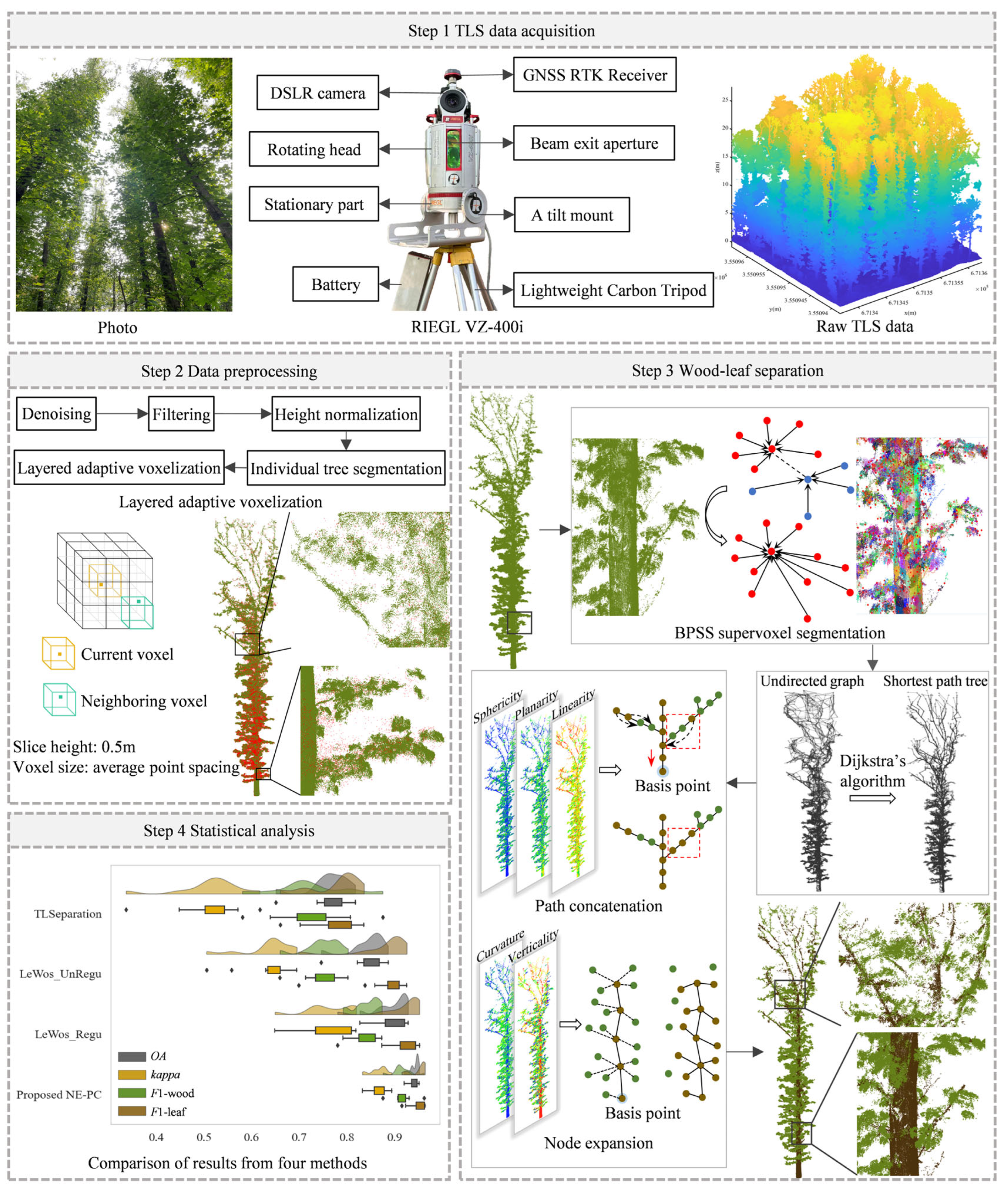

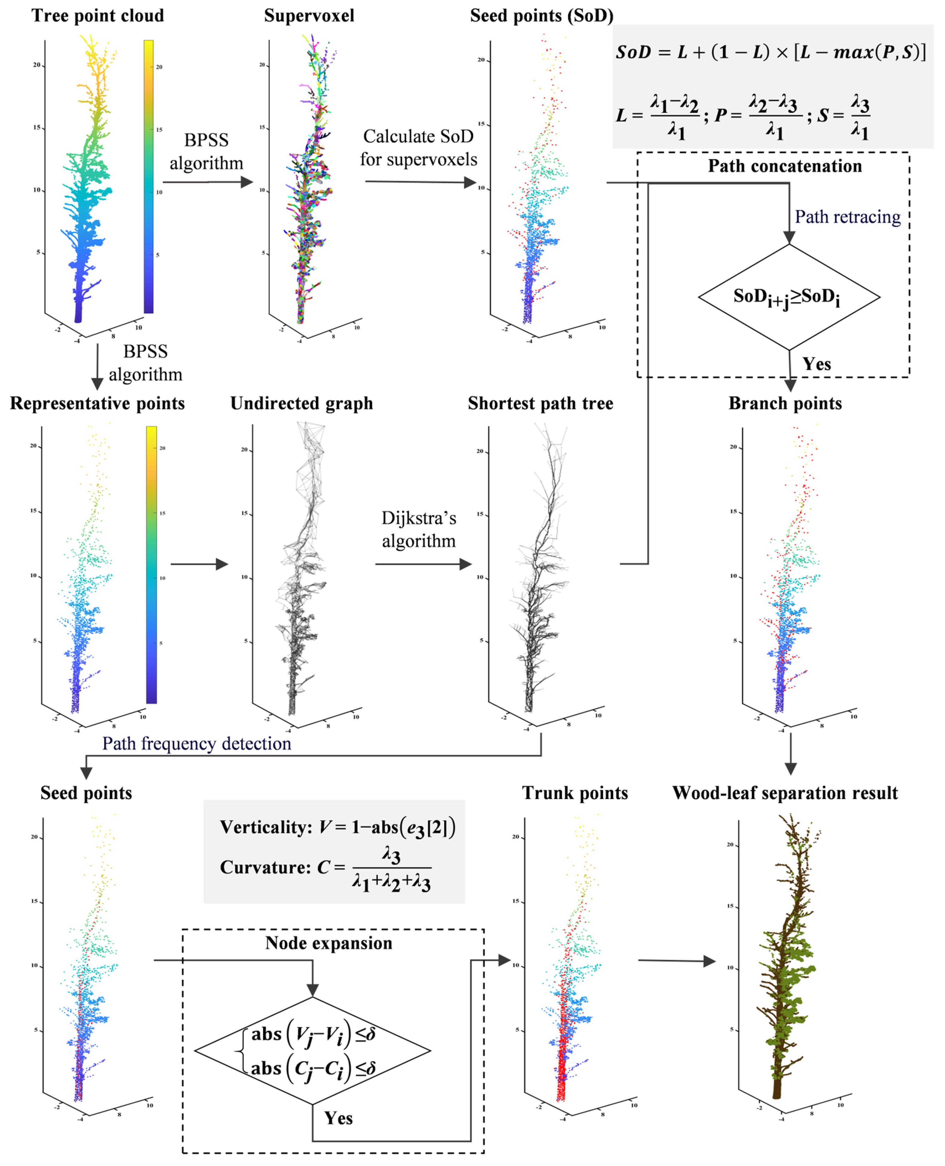

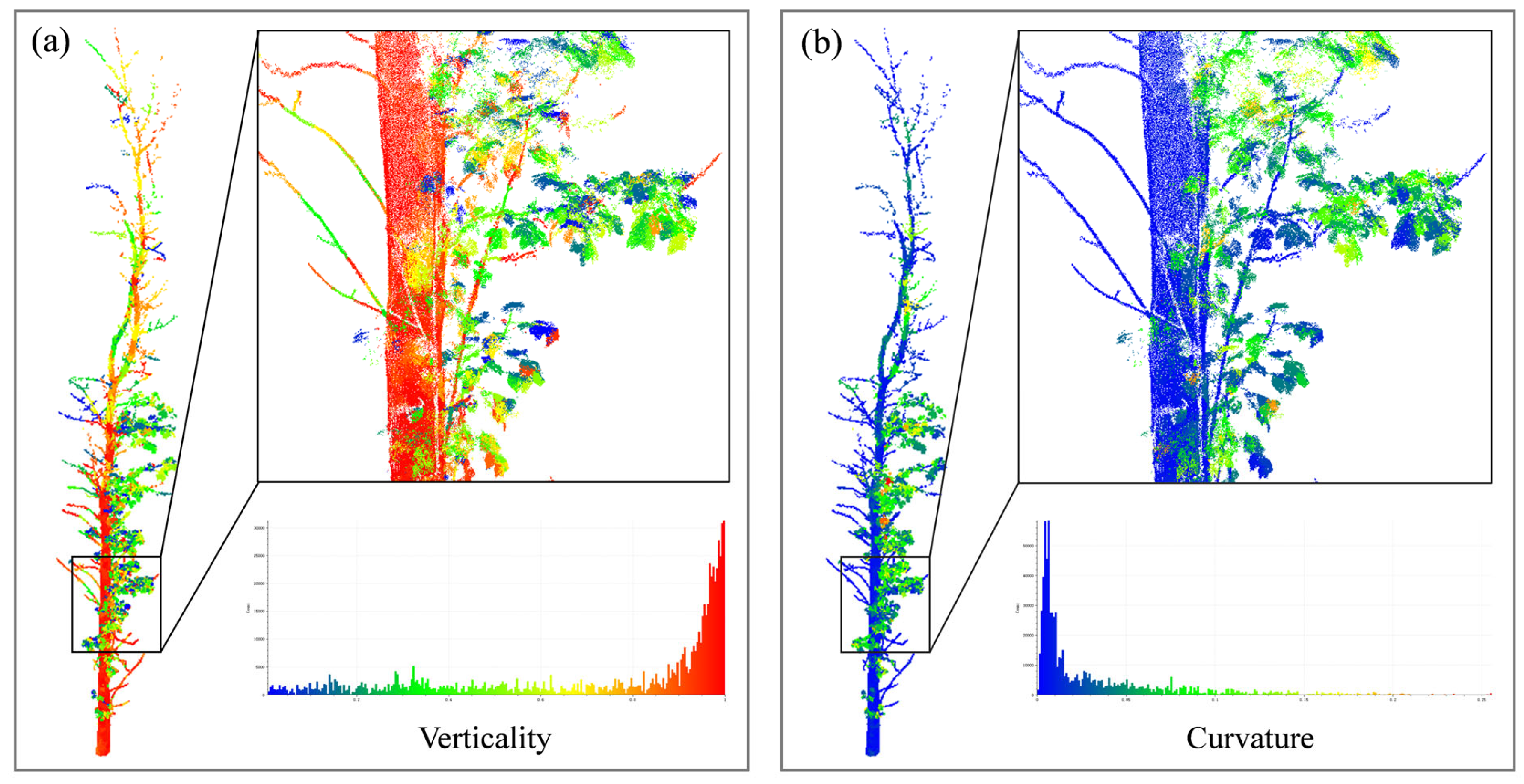

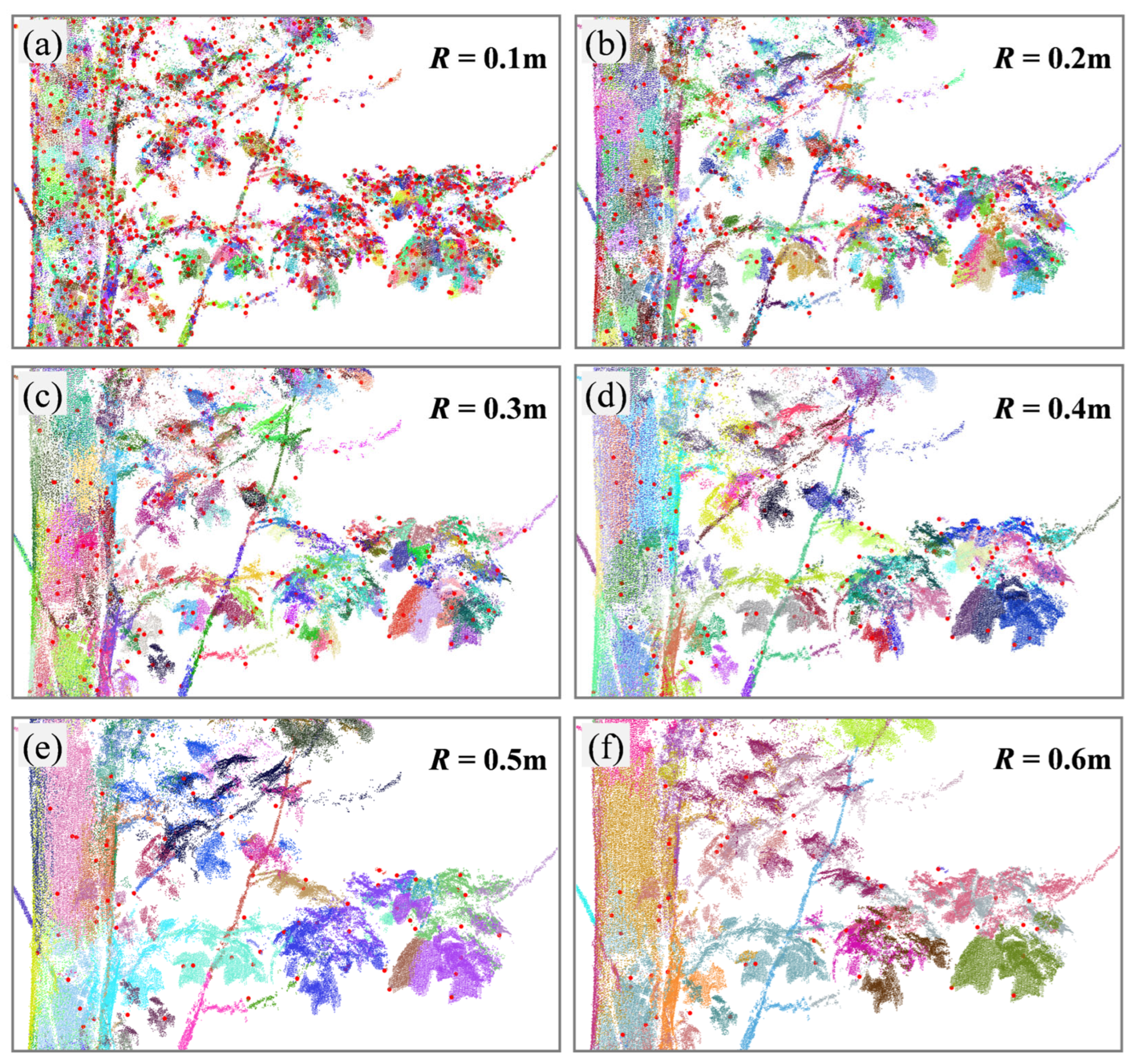
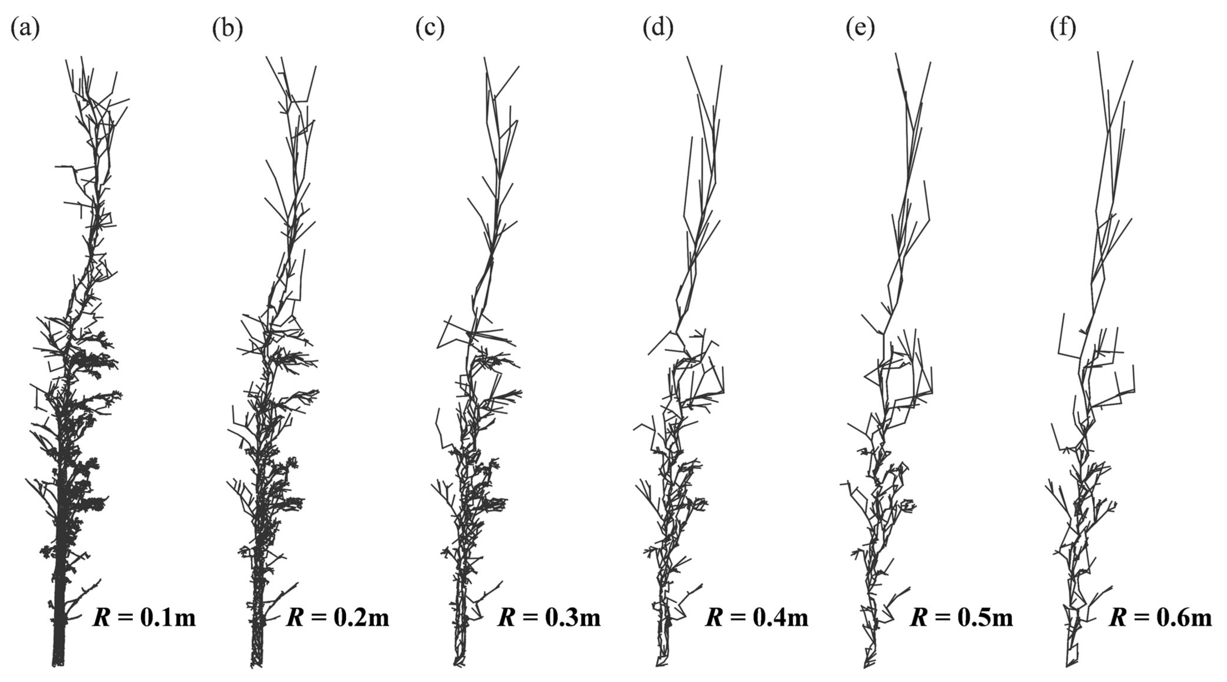
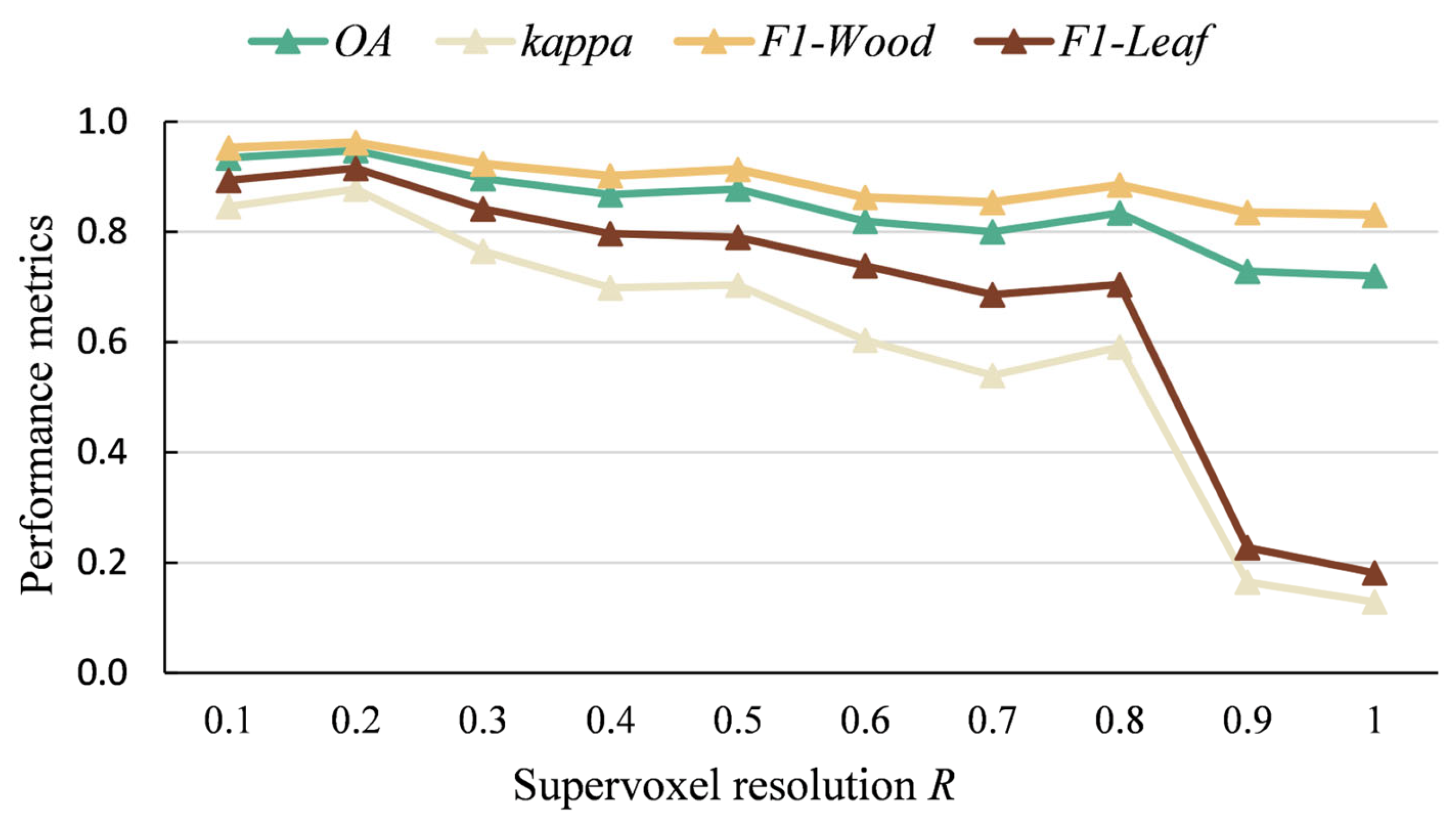
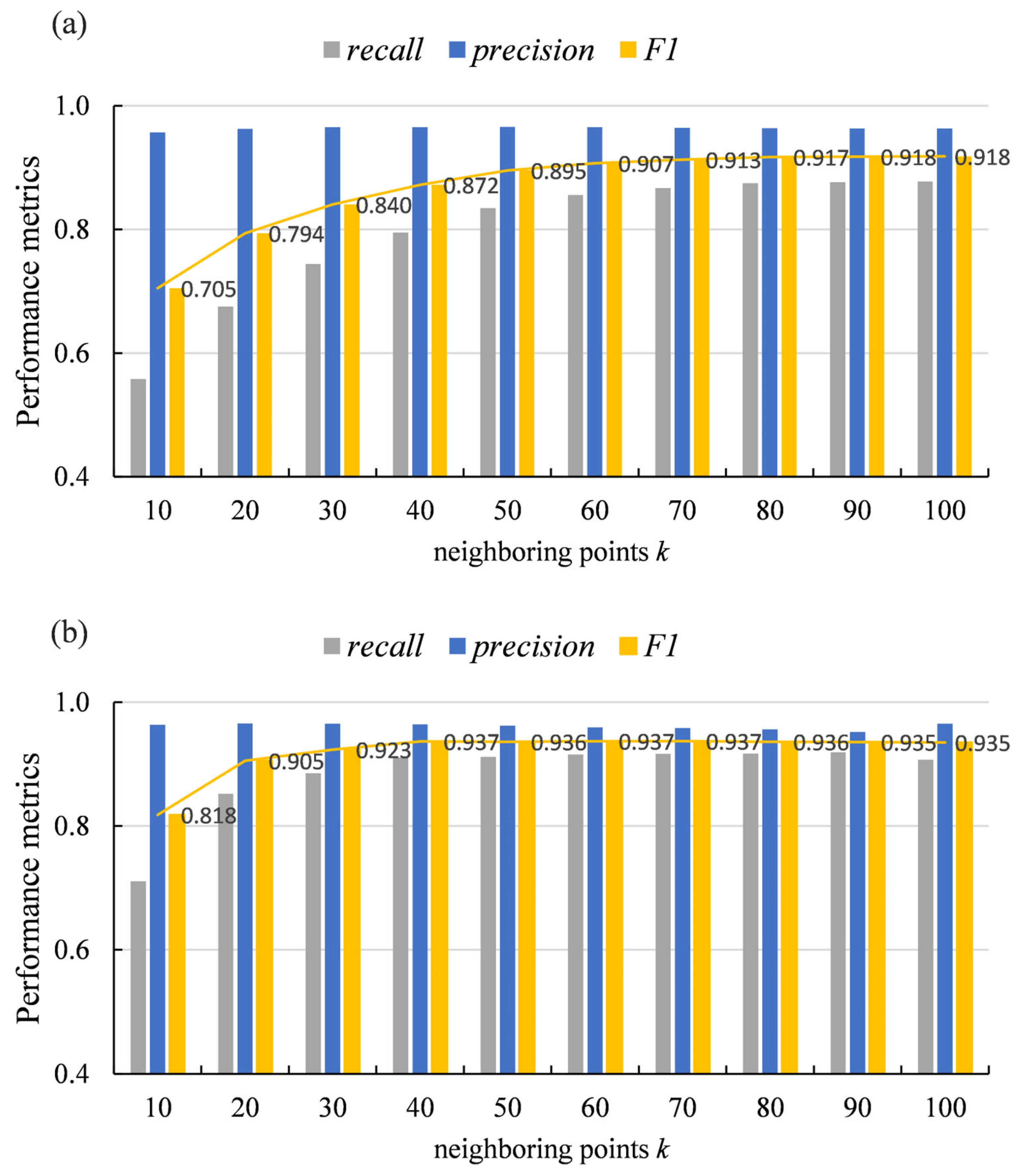
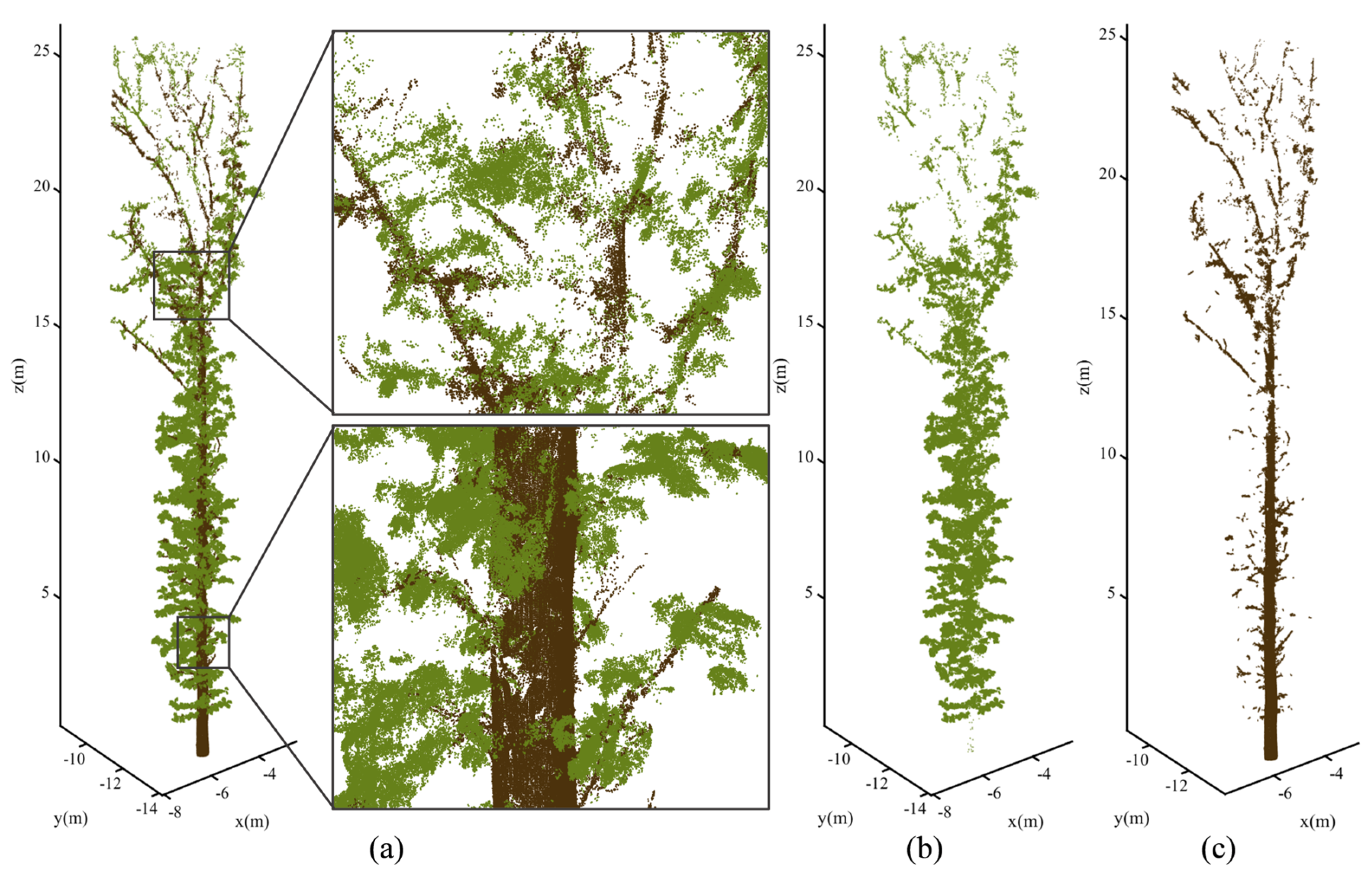
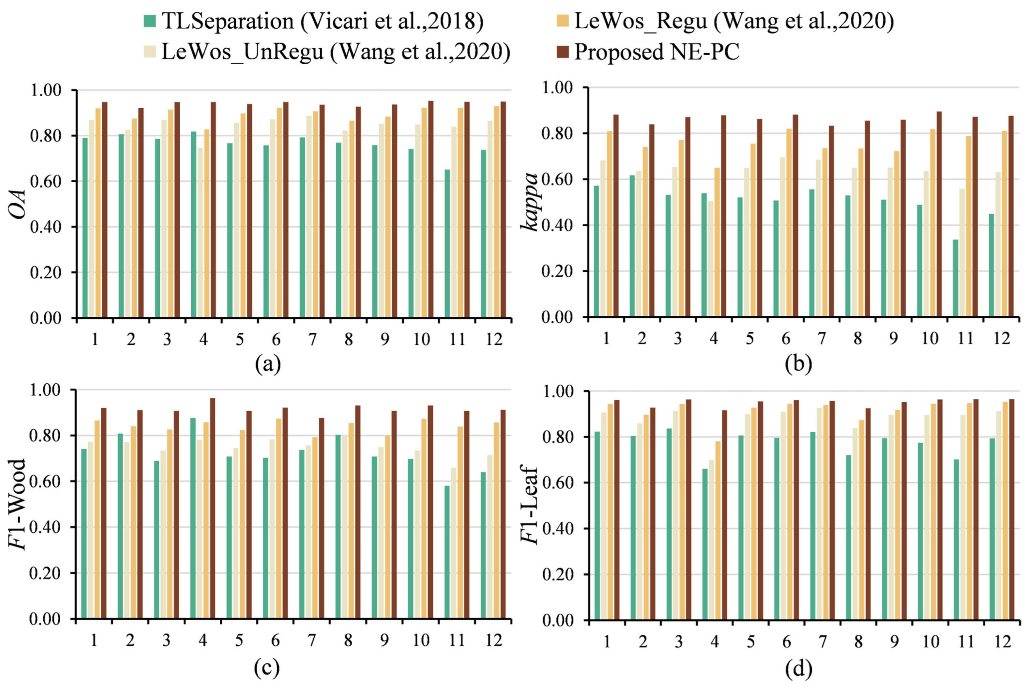
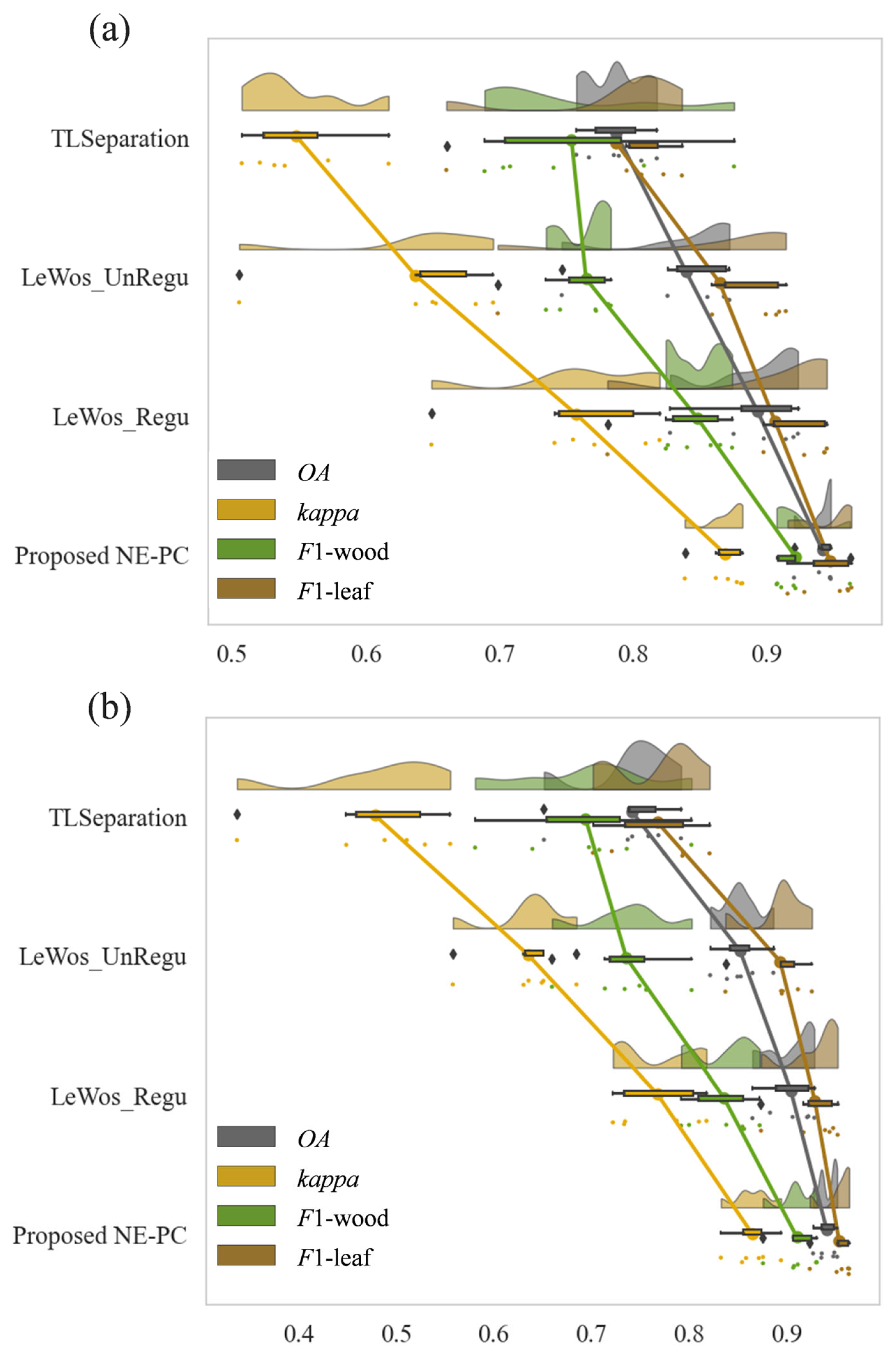
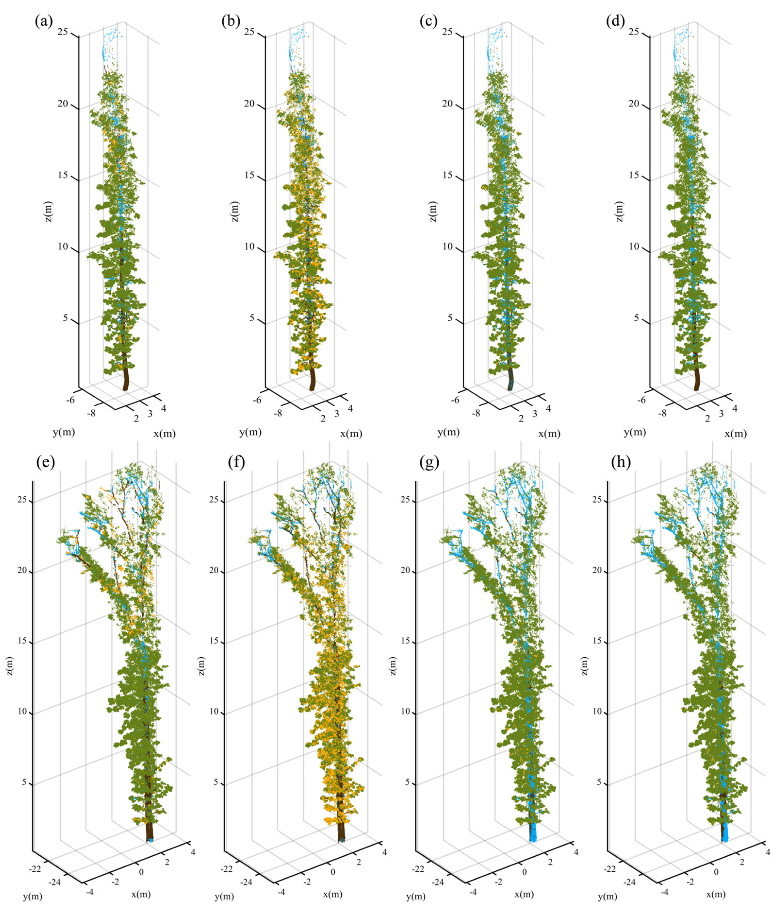
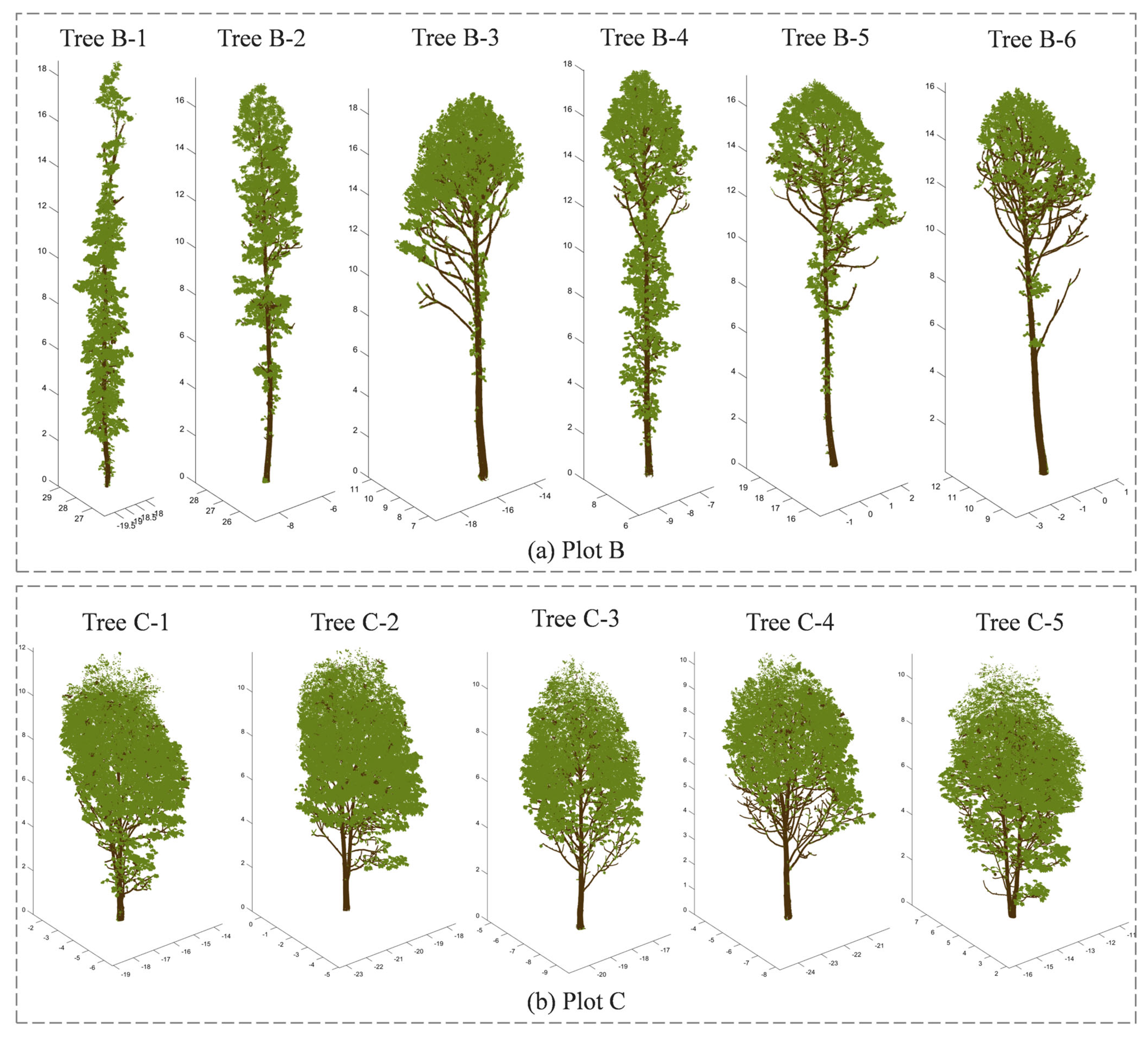
Disclaimer/Publisher’s Note: The statements, opinions and data contained in all publications are solely those of the individual author(s) and contributor(s) and not of MDPI and/or the editor(s). MDPI and/or the editor(s) disclaim responsibility for any injury to people or property resulting from any ideas, methods, instructions or products referred to in the content. |
© 2025 by the authors. Licensee MDPI, Basel, Switzerland. This article is an open access article distributed under the terms and conditions of the Creative Commons Attribution (CC BY) license (https://creativecommons.org/licenses/by/4.0/).